Ch 4 THE THEORY OF PRODUCTION

Production theory forms the foundation for the theory of supply

Managerial decision making involves four types of production decisions:

1. Whether to produce or to shut down

2. How much output to produce

3. What input combination to use

4. What type of technology to use

Ch 5

Ch 4

Production involves transformation of inputs such as capital, equipment, labor, and land into output - goods and services

In this production process, the manager is concerned with efficiency in the use of the inputs

- technical vs. economical efficiency

Two Concepts of Efficiency

Economic efficiency: occurs when the cost of producing

a given output is as low as possible

Technological efficiency: occurs when it is not possible to

increase output without increasing inputs

The objective of efficiency will provide us with some basic rules about the manner in which firms should utilize inputs to produce goods and services

You will see that basic production theory is simply an application of constrained optimization:

the firm attempts either to minimize the cost of producing a given level of output

orto maximize the output attainable with a given level of cost.

Both optimization problems lead to same rule for the allocation of inputs and choice of technology

Production Function

A production function is a table or a mathematical equation showing the maximum amount of output that can be produced from any specified set of inputs, given the existing technology

f2(x) f1(x) f0(x)

x

Q Improvement of technology f0(x) - f2(x)

Q = output x = inputs

Production Function continued

Q = f(X1, X2, …, Xk)

where

Q = output

X1, …, Xk = inputs

For our current analysis, let’s reduce the inputs to two, capital (K) and labor (L):

Q = f(L, K)

Production Table

Units of KEmployed Output Quantity (Q)

8 37 60 83 96 107 117 127 1287 42 64 78 90 101 110 119 1206 37 52 64 73 82 90 97 1045 31 47 58 67 75 82 89 954 24 39 52 60 67 73 79 853 17 29 41 52 58 64 69 732 8 18 29 39 47 52 56 521 4 8 14 20 27 24 21 17

1 2 3 4 5 6 7 8Units of L Employed

Same Q can be produced with different combinations of inputs, e.g. inputs are substitutable in some degree

All of these outputs are assumed to be technically efficient

But which one is economically efficient?

That is the question facing the DM

Short-Run and Long-Run Production

In the short run some inputs are fixed and some variable e.g. the firm may be able to vary

the amount of labor, but cannot change the amount of capital

in the short run we can talk about factor productivity

In the long run all inputs become variable e.g. the long run is the period in

which a firm can adjust all inputs to changed conditions

in the long run we can talk about returns to scale (compare latter with economies of scale, which is a cost related concept)

Short-Run Changes in ProductionFactor Productivity

Units of KEmployed Output Quantity (Q)

8 37 60 83 96 107 117 127 1287 42 64 78 90 101 110 119 1206 37 52 64 73 82 90 97 1045 31 47 58 67 75 82 89 954 24 39 52 60 67 73 79 853 17 29 41 52 58 64 69 732 8 18 29 39 47 52 56 521 4 8 14 20 27 24 21 17

1 2 3 4 5 6 7 8Units of L Employed

How much does the quantity of Q change, when the quantity of L is increased?

Long-Run Changes in ProductionReturns to Scale

Units of KEmployed Output Quantity (Q)

8 37 60 83 96 107 117 127 1287 42 64 78 90 101 110 119 1206 37 52 64 73 82 90 97 1045 31 47 58 67 75 82 89 954 24 39 52 60 67 73 79 853 17 29 41 52 58 64 69 732 8 18 29 39 47 52 56 521 4 8 14 20 27 24 21 17

1 2 3 4 5 6 7 8Units of L Employed

How much does the quantity of Q change, when the quantity of both L and K is increased?

Relationship Between Total, Average, and Marginal Product: Short-Run Analysis

Total Product (TP) = total quantity of output

Average Product (AP) = total product per total input

Marginal Product (MP) = change in quantity when one additional unit of input used

The Marginal Product of Labor

The marginal product of labor is the increase in output obtained by adding 1 unit of labor but holding constant the inputs of all other factors

Marginal Product of L:

MPL= Q/L (holding K constant)

= Q/L

Average Product of L:

APL= Q/L (holding K constant)

Short-Run Analysis of Total,Average, and Marginal Product

If MP > AP then AP is rising

If MP < AP then AP is falling

MP = AP when AP is maximized

TP maximized when MP = 0

Law of Diminishing Returns(Diminishing Marginal Product)

Holding all factors constant except one, the law of diminishing returns says that:

As additional units of a variable input are combined with a fixed input, at some point the additional output (i.e., marginal product) starts to diminish

e.g. trying to increase labor input without also increasing capital will bring diminishing returns

Nothing says when diminishing returns will start to take effect, only that it will happen at some point

All inputs added to the production process are exactly the same in individual productivity

Three Stages of Production in Short Run

AP,MP

X

Stage I Stage II Stage III

APX

MPXFixed input grossly underutilized; specialization and teamwork cause AP to increase when additional X is used

Specialization and teamwork continue to result in greater output when additional X is used; fixed input being properly utilized

Fixed input capacity is reached; additional X causes output to fall

How to Determine the Optimal Input Usage

We can find the answer to this from the concept of derived demand

The firm must know how many units of output it could sell, the price of the product, and the monetary costs of employing various amounts of the input L

Let us for now assume that the firm is operating in a perfectly competitive market for its output and its input

Example 1:

Table 7.6 Combining Marginal Revenue Product (MRP) with Marginal Labor Cost (MLC)Total Marginal Total Marginal

Labor Total Average Marginal Revenue Revenue Labor LaborUnit Product Product Product Product Product Cost Cost(X) (Q or TP) (AP) (MP) (TRP) (MRP) (TLC) (MLC) TRP-TLC MRP-MLC0 0 0 0 0 0 01 10000 10000 10000 20000 20000 10000 10000 10000 100002 25000 12500 15000 50000 30000 20000 10000 30000 200003 45000 15000 20000 90000 40000 30000 10000 60000 300004 60000 15000 15000 120000 30000 40000 10000 80000 200005 70000 14000 10000 140000 20000 50000 10000 90000 100006 75000 12500 5000 150000 10000 60000 10000 90000 07 78000 11143 3000 156000 6000 70000 10000 86000 -40008 80000 10000 2000 160000 4000 80000 10000 80000 -6000

Note: P = Product Price = $2W = Cost per unit of labor = $10000TRP = TP x P, MRP = MP x PTLC = X x WMLC = TLC / X

Optimal Decision Rule:

A profit maximizing firm operating in perfectly competitive output and input markets will be using optimal amount of an input at the point at which the monetary value of the input’s marginal product is equal to the additional cost of using that input (L)

- in other words, when MRP = MLC

Production in the Long-Run

All inputs are now considered to be variable (both L and K in our case)

How to determine the optimal combination of inputs?

To illustrate this case we will use production isoquants.

An isoquant is a curve showing all possible combinations of inputs physically capable of producing a given fixed level of output.

Example 2 Production Table

Units of KEmployed Output Quantity (Q)

8 37 60 83 96 107 117 127 1287 42 64 78 90 101 110 119 1206 37 52 64 73 82 90 97 1045 31 47 58 67 75 82 89 954 24 39 52 60 67 73 79 853 17 29 41 52 58 64 69 732 8 18 29 39 47 52 56 521 4 8 14 20 27 24 21 17

1 2 3 4 5 6 7 8Units of K Employedof L

IsoquantUnits of KEmployed

An Isoquant

Graph of Isoquant

0

1

2

3

4

5

6

7

1 2 3 4 5 6 7 X

Y

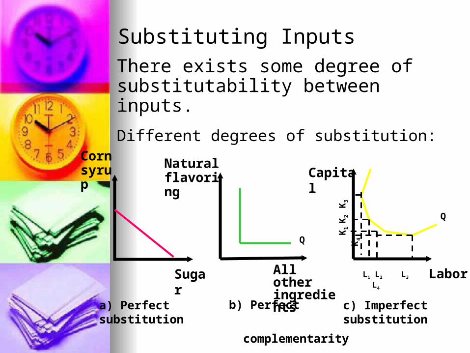
Substituting InputsThere exists some degree of substitutability between inputs.

Different degrees of substitution:

Sugar

a) Perfect substitution b) Perfect complementarity

All other ingredients

Natural flavoring

Q

Q

Capital

Labor L1 L2 L3 L4

K1 K

2 K

3

K4

Cornsyrup

c) Imperfect substitution

Substituting Inputs continued

In case the two inputs are imperfectly substitutable, the optimal combination of inputs depends on the degree of substitutability and on the relative prices of the inputs

Substituting Inputs continued

The degree of imperfection in substitutability is measured with marginal rate of technical substitution (MRTS):

MRTS = L/K

(in this MRTS some of L is removed from the production and substituted by K to maintain the same level of output)

Law of Diminishing Marginal Rate of Technical Substitution:

Table 7.8 Input Combinationsfor Isoquant Q = 52Combination L K

A 6 2B 4 3C 3 4D 2 6E 2 8

L K MRTS

-2 1 2 -1 1 1 -1 2 1/2 0 2

Law of Diminishing Marginal Rate of Technical Substitution continued

0

1

2

3

4

5

6

7

2 3 4 6 8 X

Y

X = 2Y = -1

X = 1

Y = -1

X = 1

Y =- 2

A

BC

D E

MRTS = L/K = - MPL/MPK

Units of KEmployed Output Quantity (Q)

8 37 60 83 96 107 117 127 1287 42 64 78 90 101 110 119 1206 37 52 64 73 82 90 97 1045 31 47 58 67 75 82 89 954 24 39 52 60 67 73 79 853 17 29 41 52 58 64 69 732 8 18 29 39 47 52 56 521 4 8 14 20 27 24 21 17

1 2 3 4 5 6 7 8Units of K Employedof L

MPL / MPK in Relation to MRTS (X for Y)

Combination Q L MPL K MPK MRTS (L for K) MPL / MPK

A 52 6 2B 52 4 13 3 6,5 2 2C 52 3 11 4 11 1 1D 52 2 6,5 6 13 1/2 1/2