Ch 2.5: Autonomous Equations and Population

Dynamics

• In this section we examine equations of the form dy/dt = f (y), called

autonomous equations, where the independent variable t does not appear

explicitly.

• The main purpose of this section is to learn how geometric methods can be

used to obtain qualitative information directly from differential equation

without solving it.

• Example (Exponential Growth):

• Solution: 0, rrydt

dy

rteyy 0

Lemmings Suicide Myth: Dr. Karl S. Kruszelnicki in ABC Science

• Lemmings belong to the rodents. Rodents have been around for about 57 million years. The True Lemming is about 10 cm long, with short legs and tail.

• Many of the rodents have strange population explosions. One such event in the Central Valley of California in 1926-27 had mouse populations reaching around 200,000 per hectare (about 20 mice per square metre). In France between 1790 and 1935, there were at least 20 mouse plagues. But lemmings have the most regular fluctuations - these population explosions happen every three or four years. The numbers rocket up, and then drop almost to extinction. Even after three-quarters of a century of intensive research, we don't fully understand why their populations fluctuate so much. Various factors (change in food availability, climate, density of predators, stress of overcrowding, infectious diseases, snow conditions, sunspots, etc) have all been put forward, but none completely explain what is going on.

• Indeed, this myth is now a metaphor for the behaviour of crowds of people who foolishly follow each other, lemming-like, regardless of the consequences. This particular myth began with a Disney movie.

• The myth of mass lemming suicide began when the Walt Disney movie, Wild Wilderness was released in 1958. It was filmed in Alberta, Canada, far from the sea and not a native home to lemmings. So the filmmakers imported lemmings, by buying them from Inuit children.

• Lemmings do have their regular wild fluctuations in population

and when the numbers are high, the lemmings do migrate.

• How do we set up models for fluctuations in population?

Logistic Growth

• An exponential model y' = ry, with solution y = ert, predicts unlimited

growth, with rate r > 0 independent of population.

• Assuming instead that growth rate depends on population size, replace r by a

function h(y) to obtain dy/dt = h(y)y.

• We want to choose growth rate h(y) so that

– h(y) r when y is small,

– h(y) decreases as y grows larger, and

– h(y) < 0 when y is sufficiently large, (i.e. Population decreases)

The simplest such function is h(y) = r – ay, where a > 0.

• Our differential equation then becomes

• This equation is known as the Verhulst, or logistic, equation.

, , 0dy

r ay yd

r at

Logistic Equation

• The logistic equation from the previous slide is

• This equation is often rewritten in the equivalent form

where K = r/a. The constant r is called the intrinsic growth rate, and as we

will see, K represents the carrying capacity of the population.

• A direction field for the logistic equation with

r = 1 and K = 10 is given here.

, , 0dy

r ay yd

r at

Logistic Equation: Equilibrium Solutions

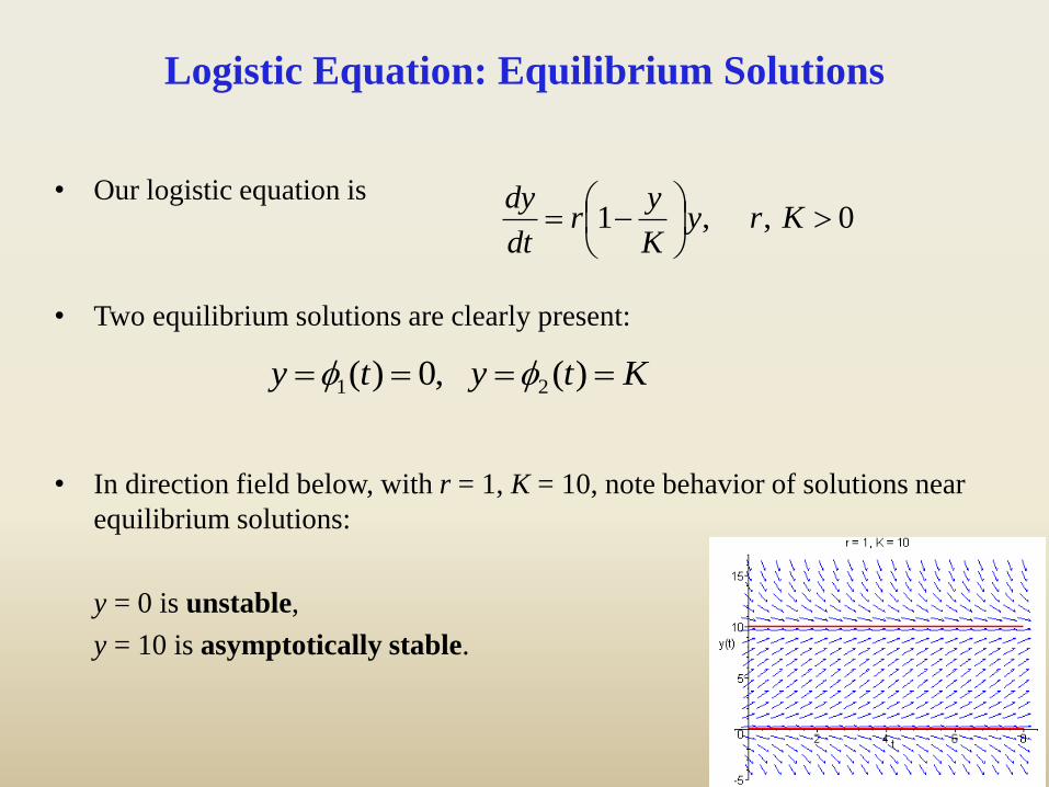
• Our logistic equation is

• Two equilibrium solutions are clearly present:

• In direction field below, with r = 1, K = 10, note behavior of solutions near

equilibrium solutions:

y = 0 is unstable,

y = 10 is asymptotically stable.

0,,1

Kry

K

yr

dt

dy

Ktyty )(,0)( 21

Autonomous Equations: Equilibrium Solutions

• Equilibrium solutions of a general first order autonomous equation y' = f (y)

can be found by locating roots of f (y) = 0.

• These roots of f (y) are called critical points.

• For example, the critical points of the logistic equation

are y = 0 and y = K.

• Thus critical points are constant functions

(equilibrium solutions) in this setting.

yK

yr

dt

dy

1

Logistic Equation: Qualitative Analysis and Curve

Sketching (1 of 7)

• To better understand the nature of solutions to autonomous

equations, we start by graphing f (y) vs y.

• In the case of logistic growth, that means graphing the following

function and analyzing its graph using calculus.

( ) 1 ( )y r

f y r y K y yK K

Logistic Equation: Critical Points (2 of 7)

• The intercepts of f occur at y = 0 and y = K, corresponding to the critical

points of logistic equation.

• The vertex of the parabola is (K/2, rK/4), as shown below.

4221

2

202

11

)(

1)(

rKK

K

Kr

Kf

KyKy

K

r

K

yy

Kryf

yK

yryf

set

Logistic Solution: Increasing, Decreasing (3 of 7)

• Note dy/dt > 0 for 0 < y < K, so y is an increasing function of t

there (indicate with right arrows along y-axis on 0 < y < K).

• Similarly, y is a decreasing function of t for y > K (indicate with

left arrows along y-axis on y > K).

• In this context the y-axis is often

called the phase line.

0,1

ry

K

yr

dt

dy

Logistic Solution: Steepness, Flatness (4 of 7)

• Note dy/dt 0 when y 0 or y K, so y is relatively flat there,

and y gets steep as y moves away from 0 or K.

yK

yr

dt

dy

1

Logistic Solution: Concavity (5 of 7)

• Next, to examine concavity of y(t), we find y'':

• Thus the graph of y is concave up when f and f ' have same sign, which occurs

when 0 < y < K/2 and y > K.

• The graph of y is concave down when f and f ' have opposite signs, which

occurs when K/2 < y < K.

• Inflection point occurs at intersection of y and line y = K/2.

2

2( ) ( ) ( ) ( )

dy d y dyf y f y f y f y

dt dt dt

(Example 1) Consider the logistic equation: K = 10

(1) Find equilibrium solutions

(2) Find a general solution of the ODE

• Hint: Use partial fractions

Solving the Logistic Equation (1 of 3)

• Provided y 0 and y K, we can rewrite the logistic ODE:

• Expanding the left side using partial fractions,

• Thus the logistic equation can be rewritten as

• Integrating the above result, we obtain

rdt

yKy

dy

1

rdtdyKy

K

y

/1

/11

CrtK

yy 1lnln

11 1 1, 1

1 1

A BAy B y K B A K

y K y y K y

Solving the Logistic Equation (2 of 3)

• We have:

• If 0 < y0 < K, then 0 < y < K and hence

• Rewriting, using properties of logs:

CrtK

yy

1lnln

CrtK

yy 1lnln

)0( where,or

111ln

0

00

0 yyeyKy

Kyy

ceKy

ye

Ky

yCrt

Ky

y

rt

rtCrt

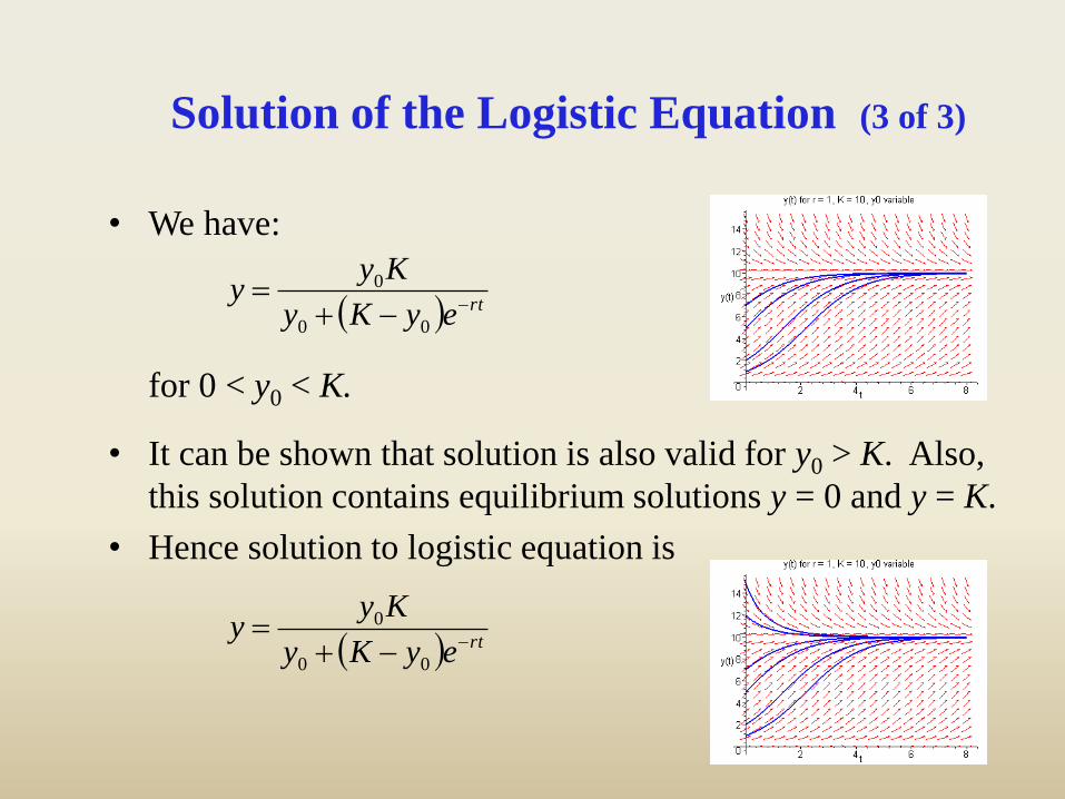
Solution of the Logistic Equation (3 of 3)

• We have:

for 0 < y0 < K.

• It can be shown that solution is also valid for y0 > K. Also,

this solution contains equilibrium solutions y = 0 and y = K.

• Hence solution to logistic equation is

rteyKy

Kyy

00

0

rteyKy

Kyy

00

0

Logistic Solution: Asymptotic Behavior

• The solution to logistic ODE is

• We use limits to confirm asymptotic behavior of solution:

• Thus we can conclude that the equilibrium solution y(t) = Kis asymptotically stable, while equilibrium solution y(t) = 0 is unstable.

• The only way to guarantee solution remains near zero is to make y0 = 0.

rteyKy

Kyy

00

0

K

y

Ky

eyKy

Kyy

trttt

0

0

00

0 limlimlim

Logistic Solution: Curve Sketching (6 of 7)

• Combining the information on the previous slides, we have:

– Graph of y increasing when 0 < y < K.

– Graph of y decreasing when y > K.

– Slope of y approximately zero when y 0 or y K.

– Graph of y concave up when 0 < y < K/2 and y > K.

– Graph of y concave down when K/2 < y < K.

– Inflection point when y = K/2.

• Using this information, we can

sketch solution curves y for

different initial conditions.

Logistic Solution: Discussion (7 of 7)

• Using only the information present in the differential equation

and without solving it, we obtained qualitative information

about the solution y.

• For example, we know where the graph of y is the steepest,

and hence where y changes most rapidly. Also, y tends

asymptotically to the line y = K, for large t.

• The value of K is known as the carrying capacity, or

saturation level, for the species.

• Note how solution behavior differs

from that of exponential equation,

and thus the decisive effect of

nonlinear term in logistic equation.

Example 2: Pacific Halibut (1 of 2)

• Let the halibut population in a region satisfies the logistic equation with r =

0.71/year, K = 80.5 x 106 kg and y0 = 0.25K.

Let y be biomass (in kg) of halibut population at time t.

(a) Set up an ODE and solve the equation

(b) Find the population 2 years later

(c) Find the time such that y() = 0.75K.

•

Ex 2: Pacific Halibut (1 of 2)

• Let y be biomass (in kg) of halibut population at time t, with r =

0.71/year and K = 80.5 x 106 kg. If y0 = 0.25K, find

(a) biomass 2 years later

(b) the time such that y() = 0.75K.

(a) For convenience, scale equation:

Then

and hence

rteyKy

Kyy

00

0

rteKyKy

Ky

K

y

00

0

1

5797.075.025.0

25.0)2()2)(71.0(

eK

y

kg 107.465797.0)2( 6 Ky

Example 1: Pacific Halibut, Part (b) (2 of 2)

(b) Find time for which y() = 0.75K.

years 095.3

75.03

25.0ln

71.0

1

13175.0

25.0

175.075.0

175.0

175.0

0

0

0

0

000

000

00

0

Ky

Ky

Ky

Kye

KyeKyKy

K

ye

K

y

K

y

eKyKy

Ky

r

r

r

r

rteKyKy

Ky

K

y

00

0

1

Critical Threshold Equation (1 of 2)

• Consider the following modification of the logistic ODE:

• The graph of the right hand side f (y) is given below.

0,1

ry

T

yr

dt

dy

Critical Threshold Equation: Qualitative

Analysis and Solution (2 of 2)

• Performing an analysis similar to that of the logistic case, we

obtain a graph of solution curves shown below.

• T is a threshold value for y0, in that population dies off or

grows unbounded, depending on which side of T the initial

value y0 is.

• See also laminar flow discussion in text.

• It can be shown that the solution to the threshold equation

is

0,1

ry

T

yr

dt

dy

rteyTy

Tyy

00

0

Logistic Growth with a Threshold (1 of

2)

• In order to avoid unbounded growth for y > T as in previous

setting, consider the following modification of the logistic

equation:

• The graph of the right hand side f (y) is given below.

KTryK

y

T

yr

dt

dy

0 and 0,11

Logistic Growth with a Threshold (2 of 2)

• Performing an analysis similar to that of the logistic case, we

obtain a graph of solution curves shown below right.

• T is threshold value for y0, in that population dies off or

grows towards K, depending on which side of T y0 is.

• K is the carrying capacity level.

• Note: y = 0 and y = K are stable equilibrium solutions,

and y = T is an unstable equilibrium solution.