Ch. 20: Keynesian Framework & IS Model

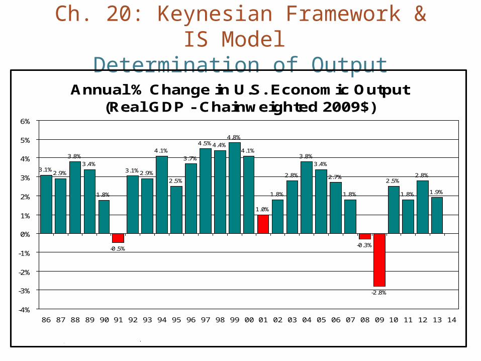
Determination of OutputAnnual % Change in U.S. Economic Output

(Real GDP - Chainweighted 2009$)

3.1%2.9%

3.8%3.4%

1.8%

3.1%2.9%

4.1%

2.5%

3.7%

4.5%4.4%4.8%

4.1%

1.0%

1.8%

2.8%

3.8%3.4%

2.7%

1.8%

-0.3%

-2.8%

2.5%

1.8%

2.8%

1.9%

-0.5%

-4%

-3%

-2%

-1%

0%

1%

2%

3%

4%

5%

6%

86 87 88 89 90 91 92 93 94 95 96 97 98 99 00 01 02 03 04 05 06 07 08 09 10 11 12 13 14

Source: Department of Commerce.

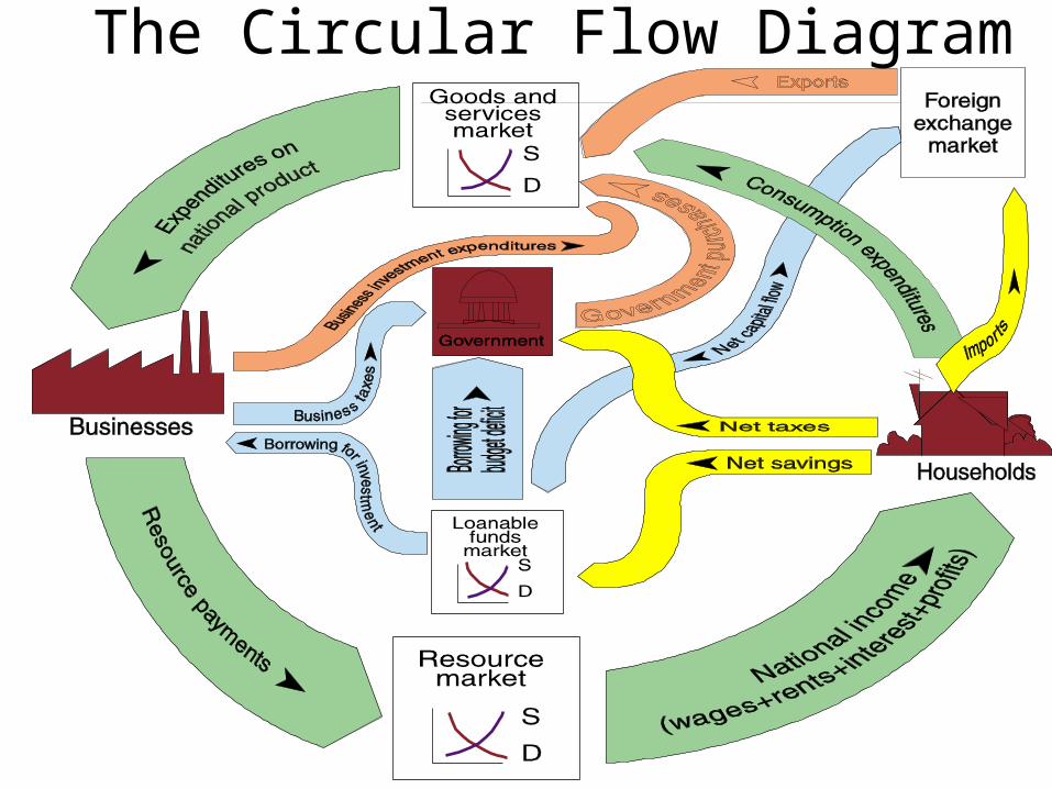
The Circular Flow Diagram

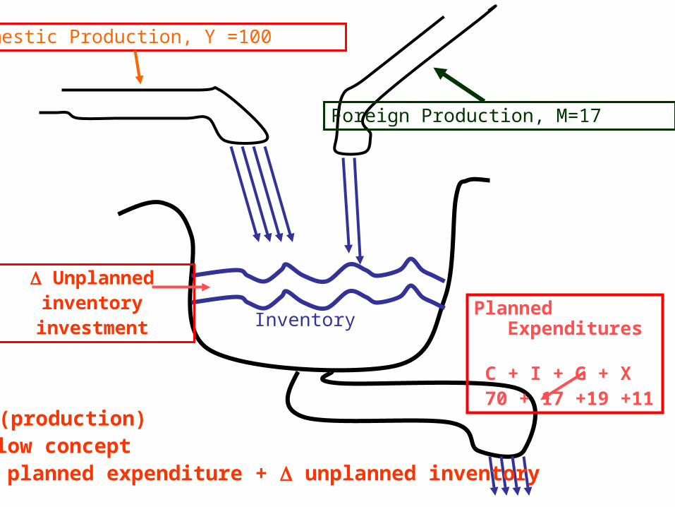
Domestic Production, Y =100

Planned Expenditures

C + I + G + X 70 + 17 +19 +11

Inventory

Foreign Production, M=17

GDP (production)• Flow concept• = planned expenditure + unplanned inventory

Unplannedinventory

investment

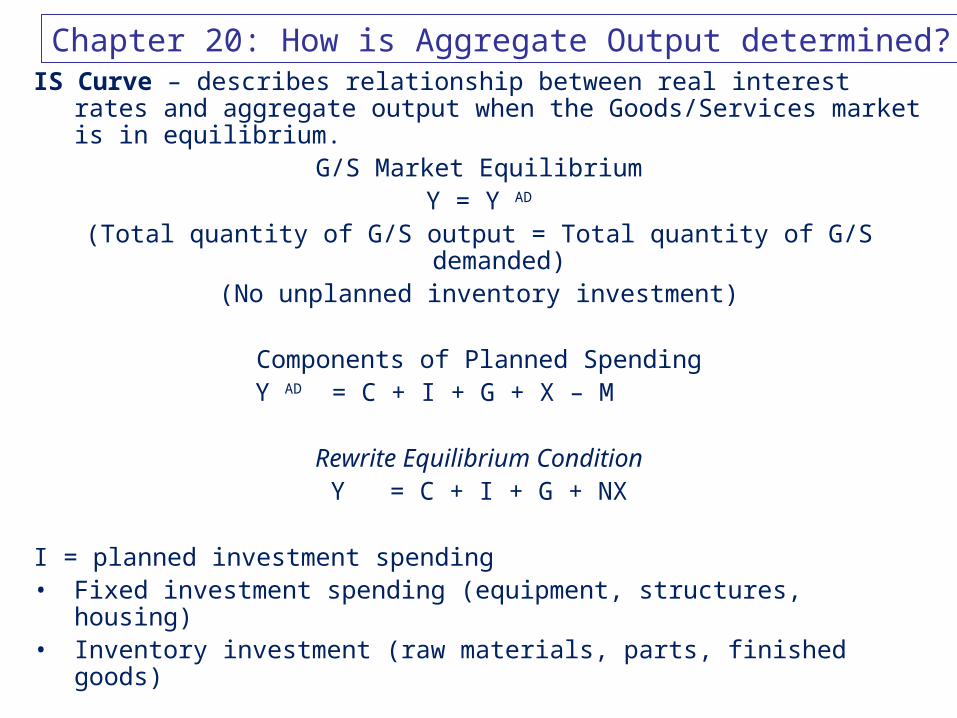
IS Curve – describes relationship between real interest rates and aggregate output when the Goods/Services market is in equilibrium.

G/S Market EquilibriumY = Y AD

(Total quantity of G/S output = Total quantity of G/S demanded)(No unplanned inventory investment)

Components of Planned SpendingY AD = C + I + G + X – M

Rewrite Equilibrium ConditionY = C + I + G + NX

I = planned investment spending• Fixed investment spending (equipment, structures, housing)• Inventory investment (raw materials, parts, finished goods)

Chapter 20: How is Aggregate Output determined?

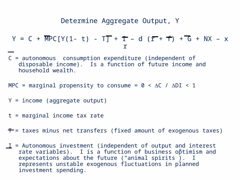
Determine Aggregate Output, Y

Y = C + MPC[Y(1- t) - T] + I – d (r + f) + G + NX – x r

C = autonomous consumption expenditure (independent of disposable income). Is a function of future income and household wealth.

MPC = marginal propensity to consume = 0 < C / DI < 1

Y = income (aggregate output)

t = marginal income tax rate

T = taxes minus net transfers (fixed amount of exogenous taxes)

I = Autonomous investment (independent of output and interest rate variables). I is a function of business optimism and expectations about the future (“animal spirits”). I represents unstable exogenous fluctuations in planned investment spending.

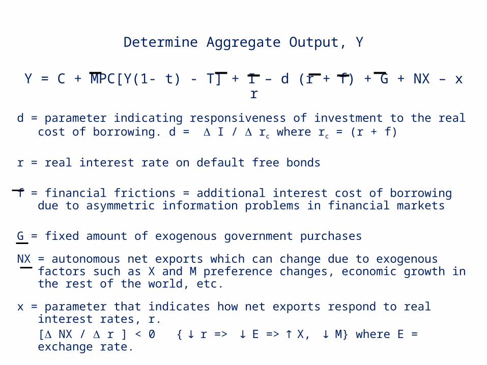
Determine Aggregate Output, Y

Y = C + MPC[Y(1- t) - T] + I – d (r + f) + G + NX – x r

d = parameter indicating responsiveness of investment to the real cost of borrowing. d = I / rc where rc = (r + f)

r = real interest rate on default free bonds

f = financial frictions = additional interest cost of borrowing due to asymmetric information problems in financial markets

G = fixed amount of exogenous government purchases

NX = autonomous net exports which can change due to exogenous factors such as X and M preference changes, economic growth in the rest of the world, etc.

x = parameter that indicates how net exports respond to real interest rates, r.[ NX / r ] < 0 { r => E => X, M} where E = exchange rate.

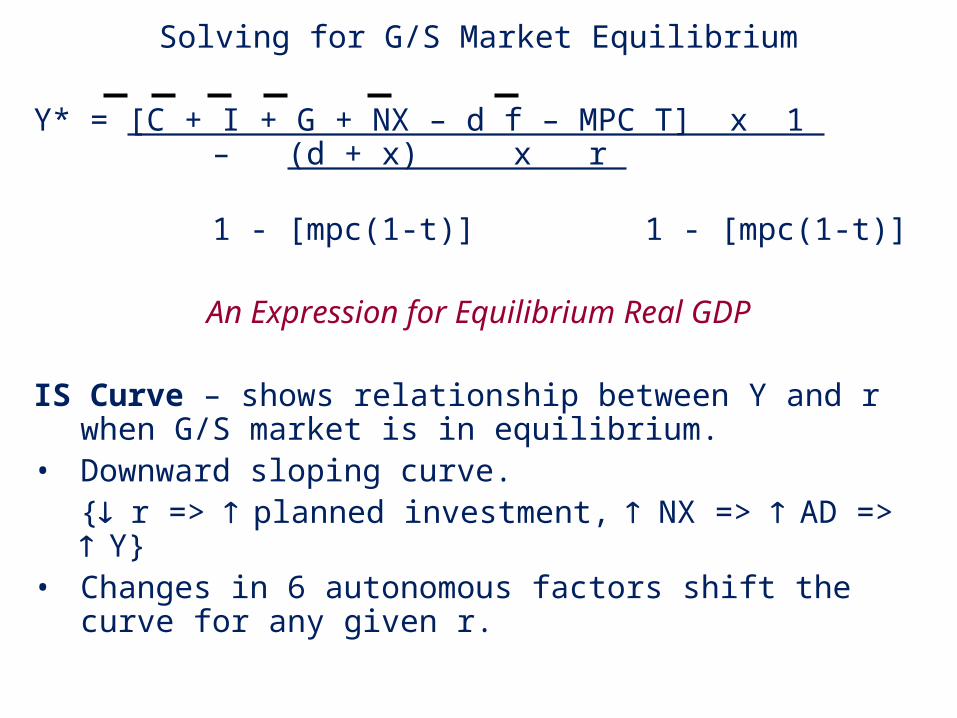
Solving for G/S Market Equilibrium

Y* = [C + I + G + NX – d f – MPC T] x 1 – (d + x) x r 1 - [mpc(1-t)] 1 - [mpc(1-t)]

An Expression for Equilibrium Real GDP

IS Curve – shows relationship between Y and r when G/S market is in equilibrium.

• Downward sloping curve.{ r => planned investment, NX => AD => Y}

• Changes in 6 autonomous factors shift the curve for any given r.

Autonomous Expenditure (Intercept) => multiple Y

Consumption:1. Household Wealth P Assets => Wealth => C2. Expected Future Income YE

t+1 => C3. Price level P => W/P (real wealth) => C4. Interest rate r =>cost of borrowing => C durables

Investment:1. E

(t+1) Animal Spirits, business confidence2. Cost of Capital Real long-term interest rates3. Taxes 4. Cash flow Retained earnings, profits

Net Exports:1. PLU.S./PLROW PL U.S. => NX2. (Y/Y)U.S. / (Y/Y)ROW (YU.S. / YROW ) => NX3. Exchange rate (e/$ ) => NX

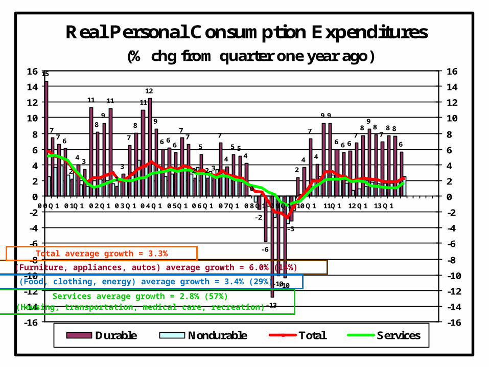
Real Personal Consumption Expenditures (% chg from quarter one year ago)

15

77

6

2

43

11

89

11

1

3

7

8

11

12

9

6 66

77

2

5

2 3

7

4

5 54

0

-2

-6

-13

-10-10

-3

2

4

7

4

9 9

6 6 67

89

87

8 8

6

-16

-14

-12

-10

-8

-6

-4

-2

0

2

4

6

8

10

12

14

16

00Q1 01Q1 02Q1 03Q1 04Q1 05Q1 06Q1 07Q1 08Q1 09Q1 10Q1 11Q1 12Q1 13Q1

-16

-14

-12

-10

-8

-6

-4

-2

0

2

4

6

8

10

12

14

16

Durable Nondurable Total Services

(Furniture, appliances, autos) average growth = 6.0% (14%)

(Food, clothing, energy) average growth = 3.4% (29%)

Services average growth = 2.8% (57%)(Housing, transportation, medical care, recreation)

Total average growth = 3.3%

10

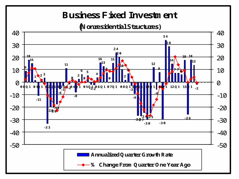
Business Fixed Investment(Nonresidential Structures)

9

1815

1

-11

2 3

-33

-20-20-18

-6-3

11

-2

0

-8

2

6

0

5

-2-2

4

1613

7

0

15

2420

10

2

7

-3

-9

-27-27-24

-30

-25

12

-6

8

-30

34

28

14

7 7 6

18

-26

18

13

-2

-50

-40

-30

-20

-10

0

10

20

30

40

00Q1 01Q1 02Q1 03Q1 04Q1 05Q1 06Q1 07Q1 08Q1 09Q1 10Q1 11Q1 12Q1 13Q1

-50

-40

-30

-20

-10

0

10

20

30

40

Annualized Quarter Growth Rate

% Change From Quarter One Year Ago

11

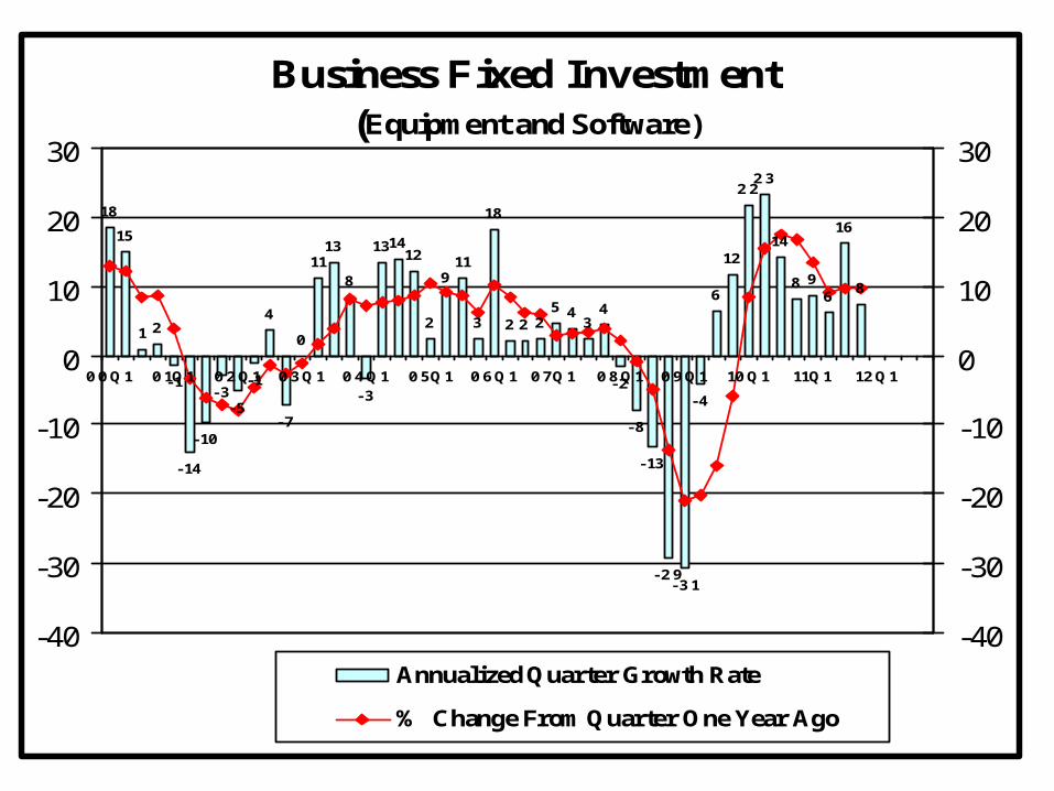
Business Fixed Investment(Equipment and Software)

18

15

1 2

-1

-14

-10

-3-5

-1

4

-7

0

1113

8

-3

131412

2

911

3

18

2 2 25 4

34

-2

-8

-13

-29-31

-4

6

12

2223

14

8 96

16

8

-40

-30

-20

-10

0

10

20

30

00Q1 01Q1 02Q1 03Q1 04Q1 05Q1 06Q1 07Q1 08Q1 09Q1 10Q1 11Q1 12Q1

-40

-30

-20

-10

0

10

20

30

Annualized Quarter Growth Rate

% Change From Quarter One Year Ago

12

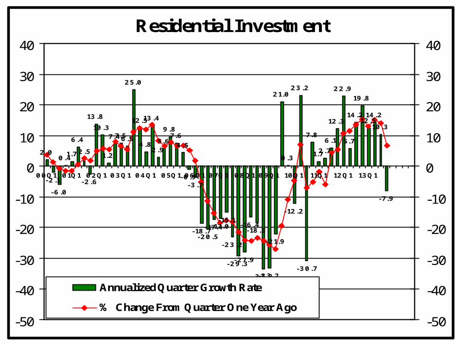
Residential Investment

2.0

-2.1

-6.0

0.41.7

6.4

2.5

-2.6

13.8

10.3

1.2

7.47.56.5

25.0

12.5

4.8

13.4

2.95.6

9.87.6

4.5

-0.9-3.7

-18.7-20.5

-17.4-17.0-15.1

-23.2

-29.3-27.9

-16.4-18.3

-33.3-33.2

-21.9

21.0

0.3

-12.2

23.2

-30.7

7.8

1.72.7

6.1

12.3

22.9

5.7

14.2

19.8

12.514.2

10.3

-7.9

-50

-40

-30

-20

-10

0

10

20

30

40

00Q1 01Q1 02Q1 03Q1 04Q1 05Q1 06Q1 07Q1 08Q1 09Q1 10Q1 11Q1 12Q1 13Q1

-50

-40

-30

-20

-10

0

10

20

30

40

Annualized Quarter Growth Rate

% Change From Quarter One Year Ago

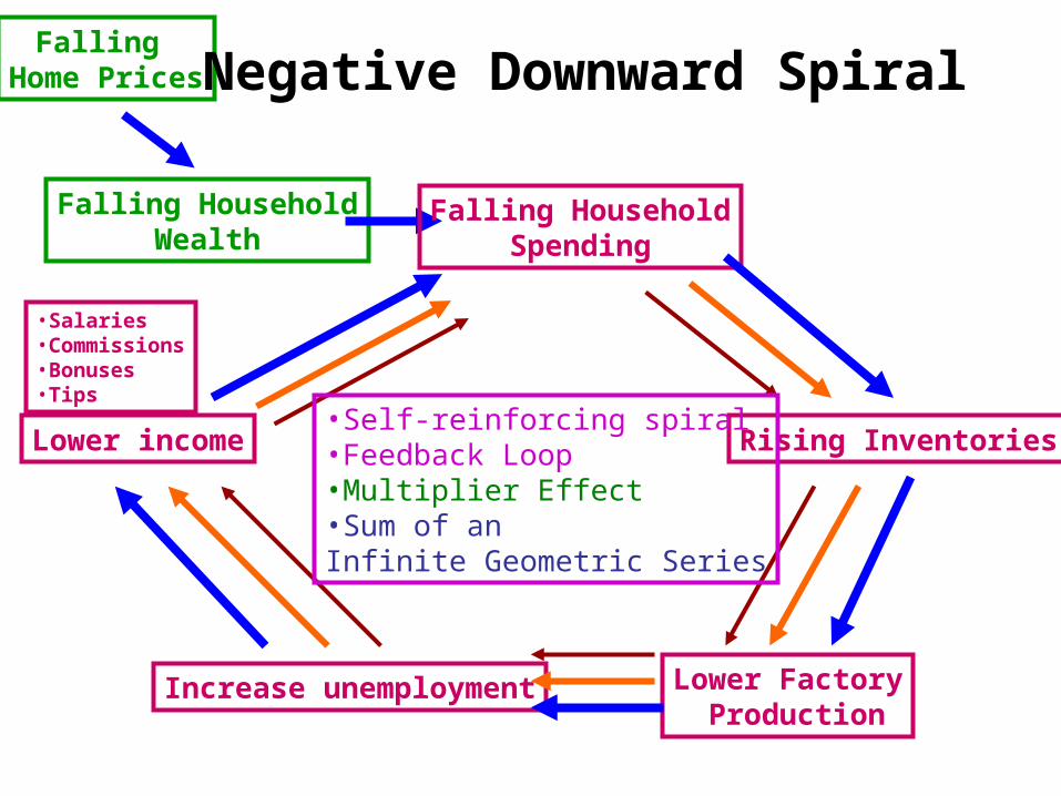
Falling Home Prices

Falling HouseholdWealth

Falling HouseholdSpending

Rising Inventories

Lower Factory Production

Increase unemployment

Lower income

Negative Downward Spiral

•Salaries•Commissions•Bonuses•Tips

•Self-reinforcing spiral•Feedback Loop•Multiplier Effect•Sum of an Infinite Geometric Series

Econ 330 Chapter 20 Homework

Due Friday, April 25

Chapter 20Questions & Applied Problems 4, 12, 14, 17, 21, 22, 24,

25