cfdanalysisoftheeffectofelbowradiusonpressuredropin...

Hindawi Publishing CorporationModelling and Simulation in EngineeringVolume 2012, Article ID 125405, 8 pagesdoi:10.1155/2012/125405

Research Article

CFD Analysis of the Effect of Elbow Radius on Pressure Drop inMultiphase Flow

Quamrul H. Mazumder

Mechanical Engineering, University of Michigan-Flint, Flint, MI 48502, USA

Correspondence should be addressed to Quamrul H. Mazumder, [email protected]

Received 9 April 2012; Accepted 24 September 2012

Academic Editor: Aiguo Song

Copyright © 2012 Quamrul H. Mazumder. This is an open access article distributed under the Creative Commons AttributionLicense, which permits unrestricted use, distribution, and reproduction in any medium, provided the original work is properlycited.

Computational fluid dynamics (CFD) analysis was performed in four different 90 degree elbows with air-water two-phase flows.The inside diameters of the elbows were 6.35 mm and 12.7 mm with radius to diameter ratios (r/D) of 1.5 to 3. The pressuredrops at two different upstream and downstream locations were investigated using empirical, experimental, and computationalmethods. The combination of three different air velocities, ranging from 15.24 to 45.72 m/sec, and nine different water velocities,in the range of 0.1–10.0 m/s, was used in this study. CFD analysis was performed using the mixture model and a commercial code,FLUENT. The comparison of CFD predictions with experimental data and empirical model outputs showed good agreement.

1. Introduction and Background

In most industrial processes, fluids are used as a medium formaterial transport. A complete knowledge of the principlesthat rule the phenomena involving fluids transportationleads to more efficient and secure systems. However, inmany industries, such as petroleum, chemical, oil, andgas industries, two-phase or multiphase flow is frequentlyobserved [1]. Multiphase flow is defined as the simultaneousflow of several phases, with the simplest case being a two-phase flow [2]. Compared to single-phase flow, the equationsassociated with two-phase flow are very complex, due to thepresence of different flow patterns in gas-liquid systems [3].A detailed discussion of two-phase flow phenomenon behav-ior is provided by Wallis [2]. The flow patterns observed inhorizontal flow are bubble, stratified, stratified wavy, slug,and annular. In vertical flows, bubble, plug, slug (or churn),annular, and wispy-annular flow patterns are present. Severalinvestigations have been reported to determine the frictionfactor and pressure drops in horizontal [4] and vertical [5]two-phase and multiphase flows [6]. The presence of thetwo-phase flow typically produces an undesirable higher-pressure drop in the piping components. In most industrial

installations, elbows are frequently used to direct the flowand provide flexibility to the system [7]. Since these fittingsare also used to install instruments that monitor the mainparameters of the industrial process, it is important to have areliable way to evaluate the pressure drop in these elbows [8].As the fluid flows through the bend, the curvature of bendcauses a centrifugal force; the centrifugal force is directedtoward the outer wall of the pipe from the momentary centerof the curvature. The combined presence of centrifugal forceand boundary layer at the wall produces the secondary flow,organized, ideally, in two identical eddies. This secondaryflow is superimposed to the mainstream along the tube axis,resulting in a helical shape streamline, flowing through thebend [9].

One of the challenges with undesirable higher-pressuredrop is the difficulty in determining a model for two-phase flow through pipe components. Despite unsuccessfulattempts to develop an accurate model for two-phase flowthrough pipe components, Chisholm [10] presented anelementary model for prediction of two-phase flow in bends,based on a liquid two-phase multiplier, for different pipediameters, r/D values, and flow rates. Detailed studiesof two-phase pressure loss have largely been confined to

2 Modelling and Simulation in Engineering

the horizontal plane. Chenoweth and Martin [11] showedthat while the two-phase pressure drop around bends washigher than in single-phase flow, it could be correlatedby an adoption of the Lockhart-Martinelli [12] model, amodel initially developed for straight pipe. The correlationclaimed to predict loss in bends and other pipe fittings.Also, at high mass velocities, agreement was achieved withthe homogeneous model. Fitzsimmons [13] presented two-phase pressure loss data for bend in terms of the equivalentlength and the ratio of the bend pressure loss to the straightpipe frictional pressure gradient; the Lockhart-Martinellimultiplier referred to the single-phase gas pressure loss inthe bend. The comparison against pressure drop in straightpipe gave a poor correlation. Sekoda et al. also used atwo-phase multiplier, referred to as a single-phase liquidpressure loss in the bend. The two-phase bend pressuredrop was found to be dependent on the r/D ratio, whilebeing independent of pipe diameters [14]. The main focusof this paper is to investigate pressure drop for two-phaseair-water mixture flow in 90 degree vertical to horizontalelbows. The first step is the prediction of the flow pattern,and then proposing an associated method of calculatingthe liquid holdup, which is used to determine the two-phase friction factor. Comparative studies proved that thesemodels are inconsistently performed, as flow conditionsvary. Therefore, the selection of the most appropriate flowcorrelation is very important in this study [15]. Reportedwork on the orientation of the plane of the bend hasoften given contrary results. Debold [16] claimed that thehorizontal bend, the horizontal to vertical upbend, and thevertical down to horizontal bend all gave the same bendpressure loss. However, a horizontal to vertical downbendhad a pressure drop that was 35% less. The correlation forelevation was assumed to follow the homogeneous modelby Debold [16], but others, such as Alves [17], ignoredhead pressure differences entirely. Peshkin [18] reportedthat horizontal to vertical downflow had about 10% morebend pressure drop than the corresponding horizontal tovertical upflow case. Kutateladze [19], by contrast, concludedthe direct opposite: that the horizontal to vertical upflowbend created the greater pressure drop. Moujaes and Aekulareported the effects of pressure drop on turning vanes in 90degree duct elbows, using CFD models in HVAC applicationsarea [20]. Due to the different approaches that can be used topredict pressure drop in elbows, the current study uses CFDanalysis in four different elbows. The CFD analysis resultswere validated using two different empirical models by Azziand Friedel [9] and Chisholm, [10] as well as experimentaldata.

2. The CFD Approach

Due to the advancements in computer hardware and soft-ware in recent years, the computational fluid dynamics tech-nique has been a powerful and effective tool to understandthe complex hydrodynamics of gas-liquid two-phase flows.The commercial CFD package, FLUENT, was used to modelthe air-water flow, in order to predict pressure drop in 90degree elbows.

Table 1: Configurations of elbows used in the study.

Pipe diameter,D (mm)

Elbow curvatureradius, r (mm)

Equivalent pipelength, Le (mm)

Elbow 1 12.7 38.1 635

Elbow 2 12.7 19.05 571.5

Elbow 3 6.35 19.05 317.5

Elbow 4 6.35 9.525 285.75

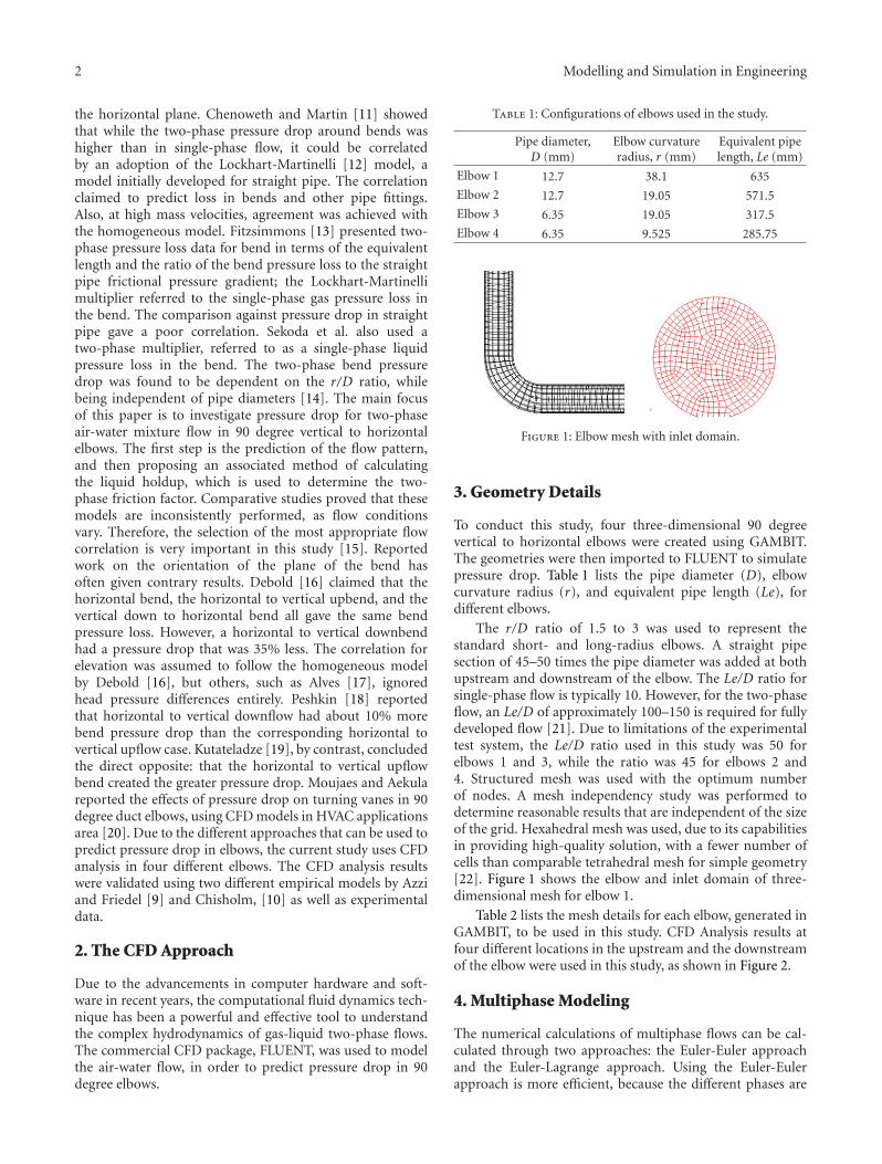
Figure 1: Elbow mesh with inlet domain.

3. Geometry Details

To conduct this study, four three-dimensional 90 degreevertical to horizontal elbows were created using GAMBIT.The geometries were then imported to FLUENT to simulatepressure drop. Table 1 lists the pipe diameter (D), elbowcurvature radius (r), and equivalent pipe length (Le), fordifferent elbows.

The r/D ratio of 1.5 to 3 was used to represent thestandard short- and long-radius elbows. A straight pipesection of 45–50 times the pipe diameter was added at bothupstream and downstream of the elbow. The Le/D ratio forsingle-phase flow is typically 10. However, for the two-phaseflow, an Le/D of approximately 100–150 is required for fullydeveloped flow [21]. Due to limitations of the experimentaltest system, the Le/D ratio used in this study was 50 forelbows 1 and 3, while the ratio was 45 for elbows 2 and4. Structured mesh was used with the optimum numberof nodes. A mesh independency study was performed todetermine reasonable results that are independent of the sizeof the grid. Hexahedral mesh was used, due to its capabilitiesin providing high-quality solution, with a fewer number ofcells than comparable tetrahedral mesh for simple geometry[22]. Figure 1 shows the elbow and inlet domain of three-dimensional mesh for elbow 1.

Table 2 lists the mesh details for each elbow, generated inGAMBIT, to be used in this study. CFD Analysis results atfour different locations in the upstream and the downstreamof the elbow were used in this study, as shown in Figure 2.

4. Multiphase Modeling

The numerical calculations of multiphase flows can be cal-culated through two approaches: the Euler-Euler approachand the Euler-Lagrange approach. Using the Euler-Eulerapproach is more efficient, because the different phases are

Modelling and Simulation in Engineering 3

Table 2: Mesh details of all four elbows.

Number ofnodes

Number of wallfaces

Number ofhexahedral cells

Elbow 1 110,558 33,344 92,738

Elbow 2 97,520 29,408 81,791

Elbow 3 21,484 8,368 16,736

Elbow 4 18,942 7,376 14,752

treated mathematically, as interpenetrating continua. Theconcept of phasic volume fraction is used in this approach,since the volume of phase cannot be occupied by the otherphases. These volume fractions are assumed to be continuousfunctions of space and time, and their sum is equal to one.For each phase, conservation equations are derived to obtaina set of new equations which have similar structure for allphases. By providing constitutive relations obtained fromthe empirical information, these sets of equations are closed.There are three available Euler-Euler multiphase models inthe fluent commercial code: the Eulerian model, the mixturemodel, and the volume of fluid model. In this study, themixture model is used, as it is relatively easy to understandfor multiphase modeling.

5. Mixture Model Theory

The mixture model can be used to model multiphase flows,by assuming the local equilibrium over short spatial lengthscales, and where the phases move at different velocities. Inaddition, the mixture model can be used to calculate non-Newtonian viscosity. It can model a number of phases bysolving the momentum, continuity, and energy equations forthe mixture, the volume fraction equation for the secondaryphases, and algebraic expression for the relative velocities.The mixture model is a good substitute for the full Eulerianmultiphase model in several cases, as the full multiphasemodel may not be feasible, due to the wide distribution ofa particular phase, when the interphase laws are unknown,or when the reliability of interphase laws is questioned.While solving a smaller number of variables than the fullmultiphase model, the mixture model can perform as wellas the full multiphase model. It uses a single-fluid approach,just like the volume of fluid model but allows for the phasesto be interpenetrating and for the phases to move at thedifferent velocities, using the concept of slip velocities.

6. Mathematical Formulation

The mixture models solve the continuity equation, momen-tum equation, energy equation, the volume fraction equationfor the secondary phases, and the algebraic expression forthe relative velocities, since the two phases are moving atdifferent velocities. The continuity, momentum, and relativevelocity equations used in the mixture model are shown inthe following section.

The mixture’s continuity equation is given by

∂

∂t

(ρm)

+∇ · (ρmvm) = 0, (1)

Location 1

Location 2

Location 3Location 4

D

r

Figure 2: Locations of CFD and experimental data.

where the mass-averaged velocity (vm) is

vm =∑n

k=1 αkρkvkρm

, (2)

and the mixture density (ρm) is given by

ρm =n∑

k=1

αkρk, (3)

where αk is volume fraction of phase k.By adding the individual momentum equations for all

phases, the mixture’s final momentum equation can beobtained, and it is given by

∂

∂t

(ρmvm

)+∇ · (ρmvmvm)

= −∇p +∇ ·[μm(∇vm +∇vTm

)]

+ ρmg + F +∇ ·⎛⎝ n∑k=1

αkρkvdr,kvdr,k

⎞⎠,

(4)

where F is the body force, n is the number of phases, and μmis the viscosity of the mixture:

μm =n∑

k=1

αkμk, (5)

where vdr,k is the drift velocity for the secondary phase k:

vdr,k = vk − vm. (6)

The relative velocity, or the slip velocity, is defined as thevelocity of a secondary phase (p), relative to the velocity ofthe primary phase (q), and can be given by

vpq = vp − vq. (7)


The mass fraction for any phase (k) is defined as

ck = αkρkρm

. (8)

The drift velocity and the relative velocity (vpq) are connectedby the following expression:

vdr,p = vpq −n∑

k=1

ckvqk. (9)

The algebraic slip formulation is used in the FLUENT’smixture model. Prescribing an algebraic relation for therelative velocity, a local equilibrium between phases shouldbe reached over short spatial length scale, according to thebasic assumption of the algebraic slip mixture model. Therelative velocity then is given by

vpq =τpfdrag

(ρp − ρm

)ρp

a, (10)

where the particle relaxation time (τp) is given by

τp =ρpd2

p

18μq, (11)

d is the diameter of the particles (or droplets or bubbles)of secondary phase, and a is the secondary-phase particle’sacceleration. The default drag function fdrag is taken fromSchiller and Naumann [19]:

fdrag ={

1 + 0.15 Re0.687 Re ≤ 1000

0.0183 Re Re > 1000,(12)

and the acceleration a is of the form

a = g − (vm · ∇) vm − ∂vm∂t

a. (13)

In the drift flux model, the acceleration of the particle isgiven by gravity and/or a centrifugal force, and, in orderto take into account the presence of other particles, theparticulate relaxation time is modified. In turbulent flows,the relative velocity should contain a diffusion term, due tothe dispersion appearing in the momentum equation for thedispersed phase. FLUENT adds this dispersion to the relativevelocity:

vpq =(ρp − ρm

)d2p

18μq fdraga− vm

αpσD∇αq, (14)

where (vm) is the mixture turbulent viscosity, and (σD) is thePrandtl dispersion coefficient.

7. Modeling Assumptions

A straight pipe section was extended at the inlet and outletboundary to evaluate the pressure drop across each elbow.In order to ensure fully developed flow, appropriate Le/Dratio was used to calculate the length of the straight section.

The standard k-ε model, with wall functions, was used inthis study, since it is the simplest of the “complete models”available in FLUENT. The model constants used for thisanalysis were C1ε = 1.44, C2ε = 1.92, Cμ = 0.09,σk = 1.0, and σε = 1.3. For the mixture parameters,slip velocity was taken into consideration, as the phaseshad a significant difference in velocities, while the no-slip boundary conditions were assumed for the wall oftubing. Due to the complex behavior of the two-phaseflow, solution strategies were followed to improve theaccuracy and convergence of the solution. The mixturecalculation was initialized with a low under relaxation factorof 0.2 for the slip velocity; calculations were performedby combinations of the SIMPLE pressure-velocity coupling.The first-order upwind discretization scheme was used forthe momentum, volume fraction, turbulent kinetic energy,and turbulent dissipation rate. The convergence criterionwas based on the residual values of the calculated variables,to ensure satisfactory accuracy, stability, and convergence.The governing equations were solved sequentially, separatefrom one another, requiring less memory in comparisonwith the coupled algorithm. SIMPLE uses the pressure-basedsegregated algorithm, which makes use of the relationshipbetween the velocity and pressure corrections, to enforcemass conservation, and to obtain the pressure field.

8. CFD Analysis

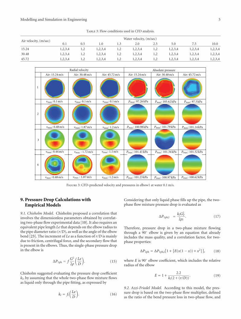
CFD analysis was performed on four different elbows, at ninedifferent water and air velocities. Thus, a total of twenty-seven different combinations of water and air velocities wereused in the study, for each elbow. Each of these conditionswas analyzed in CFD in order to accurately predict theeffect of varying the pipe diameter and r/D ratios. Dueto the limitation of the test loop system, experimentalinvestigations could not be performed for all of theseconditions. Table 3 lists all the flow conditions that were usedin the pressure loss CFD analysis. Numbers 1, 2, 3, and 4 inTable 3 represent elbows 1, 2, 3, and 4, respectively.

Cross-sectional absolute pressure and radial velocitycontours are presented in Figure 3. The left side of Figure 3shows the radial velocity contours in four locations of elbow1 at a water velocity of 0.1 m/s and air velocities of 15.24,30.48, and 45.72 m/s, respectively. Location 1 represents theinlet of the upstream pipe, while location 2 indicates theoutlet of the upstream pipe and inlet of the elbow. Similarly,location 3 indicates the outlet of elbow and inlet of thedownstream pipe, and location 4 indicates the outlet of thedownstream pipe. The top part of each individual contourrepresents the inside wall, while the bottom part of thecontour represents the outer wall of the elbow. The contourmaps were collected to locate, and study, any patterns thatwere formed. As depicted in Figure 3, the secondary flowpattern can be observed at the exit of the elbow section. Theright side of Figure 3 shows the absolute pressure profiles inthe four locations of elbow 1 at a water velocity of 0.1 m/s,and air velocities of 15.24, 30.48, and 45.72 m/s, respectively.The pressure distribution is dispersed without forming anyregular pattern.


Table 3: Flow conditions used in CFD analysis.

Air velocity, (m/sec)Water velocity, (m/sec)

0.1 0.5 1.0 1.3 2.0 2.5 5.0 7.5 10.0

15.24 1,2,3,4 1,2 1,2,3,4 1,2 1,2,3,4 1,2 1,2,3,4 1,2,3,4 1,2,3,4

30.48 1,2,3,4 1,2 1,2,3,4 1,2 1,2,3,4 1,2 1,2,3,4 1,2,3,4 1,2,3,4

45.72 1,2,3,4 1,2 1,2,3,4 1,2 1,2,3,4 1,2 1,2,3,4 1,2,3,4 1,2,3,4

Radial velocity Absolute pressure

Air: 15.24 m/s Air: 30.48 m/s Air: 45.72 m/s Air: 15.24 m/s Air: 30.48 m/s Air: 45.72 m/s

1

vmax: 0.1 m/s vmax: 0.1 m/s vmax: 0.1 m/s max: 97.26 kPa PP max: 105.62 kPa Pmax: 97.5 kPa

2

vmax: 0.48 m/s vmax: 1.87 m/s vmax: 1.2 m/s Pmax : 100.98 kPa Pmax : 101.79 kPa Pmax :101.14 kPa

3

vmax : 0.44 m/s vmax : 1.72 m/s vmax : 1.1 m/s Pmax : 101.41 kPa Pmax : 101.34 kPa Pmax : 101.52 kPa

4

vmax : 0.48 m/s vmax : 1.87 m/s vmax : 1.2 m/s Pmax : 101.23 kPa Pmax : 100.97 kPa Pmax : 100.62 kPa

Figure 3: CFD-predicted velocity and pressures in elbow1 at water 0.1 m/s.

9. Pressure Drop Calculations withEmpirical Models

9.1. Chisholm Model. Chisholm proposed a correlation thatinvolves the dimensionless parameters obtained by correlat-ing two-phase flow experimental data [10]. It also requires anequivalent pipe length Le that depends on the elbow radius tothe pipe diameter ratio (r/D), as well as the angle of the elbowbend [23]. The increment of Le as a function of r/D is mainlydue to friction, centrifugal force, and the secondary flow thatis present in the elbows. Thus, the single-phase pressure dropin the elbow is

ΔP1ph = fG2

2ρ

(Le

D

). (15)

Chisholm suggested evaluating the pressure drop coefficientkl, by assuming that the whole two-phase flow mixture flowsas liquid only through the pipe fitting, as expressed by

kl = fl

(Le

D

). (16)

Considering that only liquid phase fills up the pipe, the two-phase flow mixture pressure drop is evaluated as

ΔP1ph,l = klG2T

2ρl. (17)

Therefore, pressure drop in a two-phase mixture flowingthrough a 90◦ elbow is given by an equation that alreadyincludes the mass quality, and a correlation factor, for two-phase properties:

ΔP2ph = ΔP1ph,l[1 +

{E(x(1− x)) + x2}], (18)

where E is 90◦ elbow coefficient, which includes the relativeradius of the elbow

E = 1 +2.2

kl(2 + (r/D)). (19)

9.2. Azzi-Friedel Model. According to this model, the pres-sure drop is based on the two-phase flow multiplier, definedas the ratio of the bend pressure loss in two-phase flow, and


Elbow 1Elbow 2

Elbow 3

Elbow 4Air flowrotameter

Aircompressor

Liquid flowrotameter

Waterstorage

tank

Figure 4: Schematic of the experimental test system.

that in the single-phase liquid flow with the same total massflow rate as in [9]:

Φ2 = ΔP2ph

ΔP1ph,l, (20)

where ΔP1ph,l is the pressure drop of single-phase liquid fluid,across the same bend, defined as

ΔP1ph,l = kiGl

2

2ρl, (21)

where

ki = fi

(Le

D

), (22)

where Le/D is the dimensionless, single-phase equivalentlength, and fi is the single-phase flow pipe friction factor.According to Churchill [24], this factor can be calculated byusing the following equation:

fi = 8

((8

Re

)12

+ (Ai + Bi)−1.5

)1/12

, (23)

where

Ai =⎛⎝2.457 ln

((7

Rei

)0.9

+ 0.27ε

D

)−1⎞⎠

16

,

Bi =(

37530Rei

)16

,

Rei = ρiViD

μi.

(24)

Subscript i in the above equations can be used for eitherliquid or gas.

The two-phase flow multiplier, defined by Azzi andFriedel, is given by

Φ2 = C + 7.42Frl0.125 r

D

0.502x0.7(1− x)0.1

×⎛⎝(ρl − ρg

)ρl

⎞⎠

0.14⎛⎝(μl − μg

)μl

⎞⎠

0.12

,

C = (1− x) +

(ρlkgρgkl

)x2.

(25)

Froude number (Frl) is

Frl =(1− x2

)G2T

ρl2rg. (26)

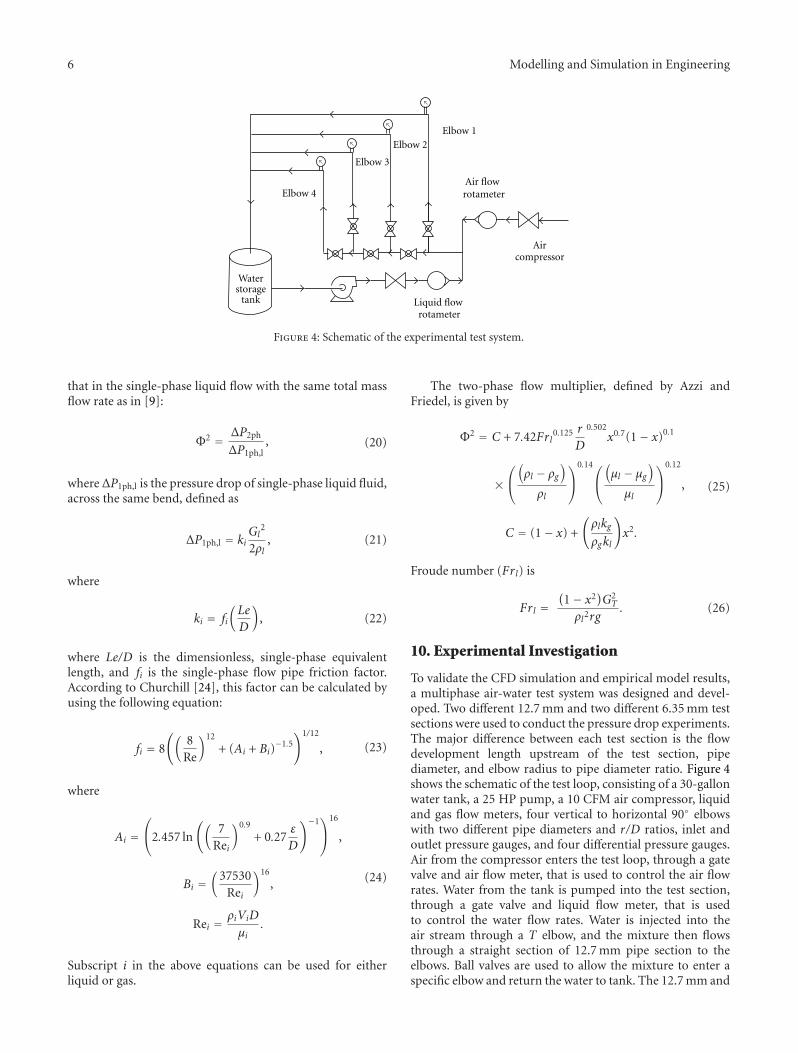
10. Experimental Investigation

To validate the CFD simulation and empirical model results,a multiphase air-water test system was designed and devel-oped. Two different 12.7 mm and two different 6.35 mm testsections were used to conduct the pressure drop experiments.The major difference between each test section is the flowdevelopment length upstream of the test section, pipediameter, and elbow radius to pipe diameter ratio. Figure 4shows the schematic of the test loop, consisting of a 30-gallonwater tank, a 25 HP pump, a 10 CFM air compressor, liquidand gas flow meters, four vertical to horizontal 90◦ elbowswith two different pipe diameters and r/D ratios, inlet andoutlet pressure gauges, and four differential pressure gauges.Air from the compressor enters the test loop, through a gatevalve and air flow meter, that is used to control the air flowrates. Water from the tank is pumped into the test section,through a gate valve and liquid flow meter, that is usedto control the water flow rates. Water is injected into theair stream through a T elbow, and the mixture then flowsthrough a straight section of 12.7 mm pipe section to theelbows. Ball valves are used to allow the mixture to enter aspecific elbow and return the water to tank. The 12.7 mm and


0.01 0.1 1 10 100 10000.01

0.1

1

10

100

1000

CFD-predicted pressure drop (kPa)

ChisholmAzziExperimentChisholmAzziExperiment

ChisholmAzziExperimentChisholmAzziExperiment

Cal

cula

ted

and

expe

rim

enta

lpr

essu

re d

rop

(kPa

)

E-1E-1

E-1E-2E-2E-2

E-3E-3E-3E-4E-4E-4

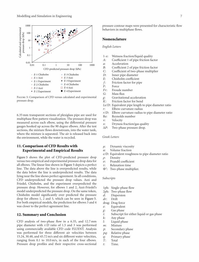
Figure 5: Comparison of CFD versus calculated and experimentalpressure drop.

6.35 mm transparent sections of plexiglass pipe are used formultiphase flow pattern visualization. The pressure drop wasmeasured across each elbow, using the differential pressuregauges hooked up across the 90 degree elbows. After the testsections, the mixture flows downstream, into the water tank,where the mixture is separated. The air is released back intothe environment, while the water is recycled.

11. Comparison of CFD Results withExperimental and Empirical Results

Figure 5 shows the plot of CFD-predicted pressure dropversus two empirical and experimental pressure drop data forall elbows. The linear line shown in Figure 5 depicts a perfectline. The data above the line is overpredicted results, whilethe data below the line is underpredicted results. The datalying near the line shows perfect agreement. In all conditions,CFD underpredicted the pressure drop values. Azzi andFriedel, Chisholm, and the experiment overpredicted thepressure drop. However, for elbows 1 and 2, Azzi-Friedel’smodel underpredicted the pressure drop. On the same token,Chisholm model significantly over predicted the pressuredrop for elbows 1, 2 and 3, which can be seen in Figure 5.For both empirical models, the prediction for elbows 3 and 4was closer to the perfect agreement line.

12. Summary and Conclusion

CFD analysis of two-phase flow in a 6.35, and 12.7 mmpipe diameter with r/D ratio of 1.5 and 3 was performedusing commercially available CFD code FLUENT. Analysiswas performed for three different air velocities between15.24, 30.48, and 45.72 m/s and six different water velocities,ranging from 0.1 to 10.0 m/s, in each of the four elbows.Pressure drop profiles and their respective cross-sectional

pressure contour maps were presented for characteristic flowbehaviors in multiphase flows.

Nomenclature

English Letters

1-x: Wetness fraction/liquid qualityA: Coefficient 1 of pipe friction factora: AccelerationB: Coefficient 2 of pipe friction factorC: Coefficient of two-phase multiplierD: Inner pipe diameterE: Chisholm coefficientf : Friction factor for pipeF: ForceFr: Froude numberG: Mass fluxg: Gravitational accelerationK : Friction factor for bendLe/D: Equivalent pipe length to pipe diameter ratior: Elbow curvature radiusr/D: Elbow curvature radius to pipe diameter ratioRe: Reynolds numberv: Velocityx: Dryness fraction/gas qualityΔP: Two-phase pressure drop.

Greek Letters

μ: Dynamic viscosityα: Volume fractionε/D: Equivalent roughness to pipe diameter ratioρ: Densityσ : Prandtl coefficientτ: Relaxation timeΦ2: Two-phase multiplier.

Subscripts

1ph: Single-phase flow2ph: Two-phase flowd: Dispersiondr: Driftdrag: Drag forcee: Equivalentg: Gas phasei: Subscript for either liquid or gas phasek: Any phasel: Liquid phasem: Mixturep: Secondary phasepq: Relative phaseq: Primary phaseT : Totalt: Time.


References

[1] S. F. Sanchez, R. J. C. Luna, M. I. Carvajal, and E. Tolentino:,“Pressure drop models evaluation for two-phase flow in 90degree horizontal elbows,” Ingenieria Mecanica Techilogia YDesarrollo, vol. 3, no. 4, pp. 115–122, 2010.

[2] G. B. Wallis, One Dimensional Two-Phase Flow, McGraw-Hill,1969.

[3] S. Benbella, M. Al-Shannag, and Z. A. Al-Anber, “Gas-liquid pressure drop in vertical internally wavy 90◦ bend,”Experimental Thermal and Fluid Science, vol. 33, no. 2, pp.340–347, 2009.

[4] J. S. Cole, G. F. Donnelly, and P. L. Spedding, “Friction factorsin two phase horizontal pipe flow,” International Communica-tions in Heat and Mass Transfer, vol. 31, no. 7, pp. 909–917,2004.

[5] S. Wongwises and W. Kongkiatwanitch, “Interfacial frictionfactor in vertical upward gas-liquid annular two-phase flow,”International Communications in Heat and Mass Transfer, vol.28, no. 3, pp. 323–336, 2001.

[6] P. L. Spedding, E. Benard, and G. F. Donnelly, “Prediction ofpressure drop in multiphase horizontal pipe flow,” Interna-tional Communications in Heat and Mass Transfer, vol. 33, no.9, pp. 1053–1062, 2006.

[7] J. Hernandez Ruız, Estudio del comportamiento de flujo defluidos en tuberıas curvas para plicaciones en metrologıa [Tesisde Maestrıa], IPN-ESIME, 1998.

[8] A. M. Chan, K. J. Maynard, J. Ramundi, and E. Wiklund,“Qualifying elbow meters for high pressure flow measure-ments in an operating nuclear power plant,” in Proceedingsof the 14th International Conference on Nuclear Engineering(ICONE ’06), Miami, Fla, USA, July 2006.

[9] A. Azzi and L. Friedel, “Two-phase upward flow 90◦ bend pres-sure loss model,” Forschung im Ingenieurwesen, vol. 69, no. 2,pp. 120–130, 2005.

[10] D. Chisholm, Two-Phase Flow in Pipelines and Heat Exchang-ers, Godwin, 1983.

[11] J. M. Chenoweth and M. W. Martin, “Turbulent two-phaseflow,” Petroleum Refiner, vol. 34, no. 10, pp. 151–155, 1955.

[12] R. W. Lockhart and R. C. Martinelli, “Proposed correlation ofdata for isothermal two-phase two-component flow in pipes,”Chemical Engineering Progress, vol. 45, no. 1, pp. 39–48, 1949.

[13] P. E. Fitzsimmons, “Two phase pressure drop in pipe compo-nents,” Tech. Rep. HW-80970 Rev 1, General Electric Research,1964.

[14] K. Sekoda, Y. Sato, and S. Kariya, “Horizontal two-phase air-water flow characteristics in the disturbed region due to a 90-degree bend,” Japan Society Mechanical Engineering, vol. 35,no. 289, pp. 2227–2333, 1969.

[15] A. Asghar, R. Masoud, S. Jafar, and A. A. Ammar, “CFDand artificial neural network modeling of two-phase flowpressure drop,” International Communications in Heat andMass Transfer, vol. 36, no. 8, pp. 850–856, 2009.

[16] T. L. Deobold, “An experimental investigation of two-phasepressure losses in pipe elbows,” Tech. Rep. HW-SA, 2564, MSc.University of Idaho, Chemical Engineering, 1962.

[17] G. E. Alves, “Co-current liquid-gas flow in a pipe-linecontactor,” Chemical Engineering Progress, vol. 50, no. 9, pp.449–456, 1954.

[18] M. A. Peshkin, “About the hydraulic resistance of pipe bendsto the flow of gas-liquid mixtures,” Teploenergetika, vol. 8, no.6, pp. 79–80, 1961.

[19] S. S. Kutateladze, Problems of Heat Transfer and Hydraulics ofTwo-Phase Media, Pergamon Press, Oxford, UK.

[20] S. F. Moujaes and S. Aekula, “CFD predictions and experimen-tal comparisons of pressure drop effects of turning vanes in 90◦

duct elbows,” Journal of Energy Engineering, vol. 135, no. 4, pp.119–126, 2009.

[21] Q. H. Mazumder, S. A. Shirazi, and B. S. McLaury, “Predictionof solid particle erosive wear of elbows in multiphase annularflow-model development and experimental validation,” Jour-nal of Energy Resources Technology, vol. 130, no. 2, Article ID023001, 10 pages, 2008.

[22] I. Fluent, Fluent 6. 3 User Guide, Fluent Inc., Lebanon, NH,USA, 2002.

[23] N. P. Cheremisinoff, Ed., Encyclopedia of Fluid Mechanics: GasLiquid Flows, vol. 3, Gulf Publishing Company, 1986.

[24] S. W. Churchill, “Friction equation spans all fluid flowregimes,” Chemical Engineering, vol. 84, no. 24, pp. 91–92,1977.

International Journal of

AerospaceEngineeringHindawi Publishing Corporationhttp://www.hindawi.com Volume 2010

RoboticsJournal of

Hindawi Publishing Corporationhttp://www.hindawi.com Volume 2014


Active and Passive Electronic Components

Control Scienceand Engineering

Journal of



RotatingMachinery


Hindawi Publishing Corporation http://www.hindawi.com

Journal ofEngineeringVolume 2014

Submit your manuscripts athttp://www.hindawi.com

VLSI Design



Shock and Vibration


Civil EngineeringAdvances in

Acoustics and VibrationAdvances in



Electrical and Computer Engineering

Journal of

Advances inOptoElectronics

Hindawi Publishing Corporation http://www.hindawi.com

Volume 2014

The Scientific World JournalHindawi Publishing Corporation http://www.hindawi.com Volume 2014

SensorsJournal of


Modelling & Simulation in EngineeringHindawi Publishing Corporation http://www.hindawi.com Volume 2014


Chemical EngineeringInternational Journal of Antennas and

Propagation




Navigation and Observation



DistributedSensor Networks


cfdanalysisoftheeffectofelbowradiusonpressuredropin...

Documents