cfd study of scour gap effect around a pipe - ysrgst.org · 1st international conference of recent...

1st International Conference of Recent Trends in Information and Communication Technologies

*Corresponding author: [email protected]

Computational Fluid Dynamic (CFD) Study of Scour Gap Effect around a

Pipe Abbod Ali1, P. Ganesan1, Shatirah Akib2,*

1 Department of Mechanical Engineering, Faculty of Engineering, University of Malaya Kuala Lumpur,

Malaysia-50603,

2 Department of Civil Engineering, Faculty of Engineering, University of Malaya, Kuala

Lumpur, Malaysia-50603, Phone: +03-79677651

Abstract

A numerical investigation of incompressible and transient flow around circular pipe has been carried out

at different five phases. Flow equations such as Navier-Stocks and continuity equations have been solved

using finite volume method. Unsteady horizontal velocity and kinetic energy square root profiles are

plotted using standard k model and Large Eddy Simulation (LES) model and their sensitivity is

checked against published experimental results. Flow parameters such as drag coefficient and lift

coefficient are studied and presented graphically to investigate the flow behavior around an immovable

pipe and scoured bed. The standard k-ε model and LES both can predict accurate results in comparison to

other turbulence models

Keywords: CFD; unsteady flow; flow around circular pipe; turbulence models; vortex shedding;

scouring; interfacial forces; vortex induced vibration (VIV).

IRICT 2014 Proceeding

12th -14th September, 2014, Universiti Teknologi Malaysia, Johor, Malaysia

Abbod Ali et. al. /IRICT (2014) 561-574 562

1 Introduction

Scouring can be defined as the erosion of sand bed sediment surrounding the obstruction i.e.,

bridge piers and abutments when the obstruction is exposed to continuously strong flow field

or flood events [1-4].The sand bed can be undermined due to the normal flow field subjected

to the obstruction under flow conditions by which its rate increases with larger flow events. In

other words, scouring is basically caused when the foundation of the bed is swept away under

flood conditions in which the flow around the obstruction accelerates and induces high shear

stress over the seabed surface [5, 6]. The resulted reduction of the sand bed around the pier

and abutment below the normal and natural river level is called the scour depth. A scour hole is

a pit or void that forms as a result of the sand bed sediment removal from the river bed [7].

Cylindrical bridge piers are the mostly used hydraulic structures in coastal, offshore and river

engineering. Thus, scour around bridge piers and submarines prediction is attracted by the

hydraulic and ocean engineers. Local scouring surrounding the bridge piers is considered to

be one of the mostly common causes of bridge pier failure [8-10].The local scour around river

hydraulic structures is a disaster mitigation of the engineering structure [11, 12]. It leaves them

in unsafe conditions requiring maintenance and occasionally results in loss of life. Damage of

hydraulic structure because of local scouring is a global concern, and it has been studied by

many researchers experimentally and numerically for several decades such as [13, 14].

Mao [22] studied the interaction between a pipeline and erodible bed. Author observed the scour

around horizontal cylinders in steady current and wave conditions, as well as with different

Reynolds numbers (Re), Shields parameters, and pipeline gaps. These experiments examined

scour features such as shape and size of the scour hole, and the time scale of the scour

formation. Later this work was further investigated by Jensen [23]. They investigated

experimentally the flow around a pipeline placed initially on a flat, erodible bed at five

characteristics stages of a progressive process in currents. The results showed that as the scour

develops with time and space, the mean flow field and turbulence around and the forces on a

pipeline undergo considerable changes. This study aims to investigate the effect of turbulence

models on the flow field behavior at different five scouring phases and study the effect of

scouring on flow parameters such as drag coefficient C𝑑 , lift coefficient Cl.


2 Methodology

2.1 Geometrical structure and Boundary conditions

Fig. 1 shows the schematic of the two dimensional (2D) geometrical domain used in the

present study along with the corresponding boundary conditions. A logarithmic velocity

profile as presented in Fig. 3 is created using user-defined functions (UDF) in Fluent based

on the following formulation [24].

Figure 1: Geometrical model of computational domain and boundary conditions

Figure 2: The grid for model calculation


lny

U

K y

u

(1)

Where U is an approach velocity (m/s), u

is friction (or shear) velocity, 1 2

u

(m/s) , y= water (or flow) depth (m) and y is roughness height (m).

The velocity profile is applied at the inlet. The profile from the presented CFD model is

compared with that from the experimental study of Dudley [25] for consistency, see Fig. 3.

Zero pressure outlet boundary condition is applied at the flow exist. The water surface (top wall)

is set as a symmetry boundary condition. No-slip boundary condition is applied on the pipe

surface and the scour bed. Gravity acts in the negative y-direction.

Figure3: Comparison of the horizontal logarithmic velocity-inlet (𝑼𝟎) in the total water depth between

present numerical investigation and experimental work of Dudley RD [25].

2.2 Governing equations

The continuity and the momentum equations for the present case are as given below:

Continuity equation:

0u

x y

(2)

X-component of the momentum equation:

2 2

2 2

u u u uu

x y x x y

(3)


Y-component of the momentum equation:

2 2

2 2u g

x y y x y

(4)

2.3 Turbulence modeling

Turbulence models of two-equation k and Large Eddy Simulation (LES) models are used

in the present research and their results are compared with experimental data from the

literature.

2.3.1 k- 𝜺 models

Two-equation k- 𝜀 models, turbulent kinetic energy k and turbulent dissipation 𝜀, are the

simplest and the most widely used models among all turbulence models that aim to study the

effect of turbulence in the flow. Two-equation model signifies that it includes two extra

transport equations to represent turbulence properties of the flow. There are three different

models that are derived from k- 𝜀 model standard k- 𝜀 model, Realizable k- 𝜀 model and

Renomalization Group model (RNG). Despite of having the two general equations, these

turbulence models use the different ways to calculate the principle form of the eddy viscosity

equation

2.3.2 Large Eddy Simulation (LES)

A large-eddy simulation (LES) model explicitly calculates the large-eddy field and

parameterizes the small eddies. The large eddies in the atmospheric boundary layer are

believed to be much more important and insensitive to the parameterization scheme for the

small eddies. In large-eddy simulation (LES), the large three-dimensional unsteady turbulent

motions are directly resolved while the smaller scale motions are modeled. In terms of


computational effort LES lies between RANS and DNS, and it can be expected more accurate

and reliable than Reynolds-stress models for flows where large-scale unsteadiness is significant

[26-30].

2.3.2.1 Smagorinsky-Lilly model

The first SGS model developed was the Smagorinsky-Lilly model, which was developed

by Smagorinsky. It models the eddy viscosity as:

2 2

2T s g ij jj s g

v C A S S C A S (5)

Where g

the grid is size and s

C is a constant. This method assumes that the energy

production and dissipation of the small scales are equilibrium.

2.4 Numerical methods

The commercial CFD software FLUENT 14.0 [31] which is based on Finite Volume Method

(FVM) is used to solve the Large Eddy Simulations (LES) equations for an incompressible

flow. The transport governing equations are discretized using the second order upwind spatial

discretization method. The Pressure-Implicit with Splitting of Operators (PISO) scheme was

used for the coupling of the pressure and the velocity fields. The under-relaxation factor of all

the components, such as velocity components and pressure correction is kept at 0.3. The scaled

residuals of 1×10-6 are set as the convergence criteria for the continuity and momentum

equations. Transient model based on implicit scheme with a time step were used in the current

numerical study. The typical wall treatment function y+ (= yUτ/ν) value of the first node in all

turbulence model near the bed profile is less than 1


2.5 Simulation cases

A total of 7 cases were simulated in the present study, see Table 1. In the first part of this

study, the effect of different turbulence models such as standard k-ε model and Large Eddy

Simulation (LES) model on horizontal velocity and kinetic energy square root has been

investigated. For studying this effect, we have adopted the domain proposed by Jensen e

al.[23] to validate the results of Mao et al. [22]. This domain is of 0.5 m length and 0.1 m

height with pipe diameter of 0.03 m. Turbulence models were tested for scour gap at time 0

min, 1 min, 6 min, 30 min, and 300 min and four positions (X/D = -3.0, 1.0, 4.0, and 8.0) in-

front and behind the pipe. Qualitatively the results of a particular turbulence model were same

for all scour gaps, so, the results of Cases (1-2) for scour gap at time 0 min are presented.

Consequently, the turbulence model that reproduces a similar result as of experimental

investigation of Jensen et al. is chosen for all further simulation cases in the current study.

In the second part of this paper, a parametric study has been carried out by using five bed profiles

suggested by Mao [22] at 0 min, 1 min, 6 min, 30 min, and 300 min. Five simulation cases (7-

11) were run to obtain the drag coefficient d

C and lift coefficient l

C around the pipe with

different gaps at position X/D=0 using LES turbulence model.

Table 1: Simulation cases

2.6 Mesh independence and time step test

The computational mesh constructed by FLEUNT is based on the square grid. The grid used in

this simulation is a variable 0.001m grid along a scoured bed wall and around the cylinder


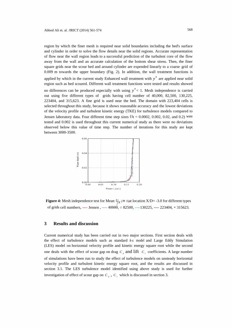
region by which the finer mesh is required near solid boundaries including the bed's surface

and cylinder in order to solve the flow details near the solid regions. Accurate representation

of flow near the wall region leads to a successful prediction of the turbulent core of the flow

away from the wall and an accurate calculation of the bottom shear stress. Then, the finer

square grids near the scour bed and around cylinder are expended linearly to a coarse grid of

0.009 m towards the upper boundary (Fig. 2). In addition, the wall treatment functions is

applied by which in the current study Enhanced wall treatment with 𝑦+ are applied near solid

region such as bed scoured. Different wall treatment functions were tested and results showed

no differences can be produced especially with using 𝑦+< 1. Mesh independence is carried

out using five different types of grids having cell number of 40,000, 82,500, 130,225,

223404, and 315,623. A fine grid is used near the bed. The domain with 223,404 cells is

selected throughout this study, because it shows reasonable accuracy and the lowest deviations

of the velocity profile and turbulent kinetic energy (TKE) for turbulence models compared to

Jensen laboratory data. Four different time step sizes (∆t = 0.0002, 0.002, 0.02, and 0.2) were

tested and 0.002 is used throughout this current numerical study as there were no deviations

observed below this value of time step. The number of iterations for this study are kept

between 3000-3500.

Figure 4: Mesh independence test for Mean U x m s at location X/D= -3.0 for different types

of grids cell numbers, ---- Jensen , ---- 40000, ○ 82500, ----130225, ---- 223404, × 315623.

3 Results and discussion

Current numerical study has been carried out in two major sections. First section deals with

the effect of turbulence models such as standard k-ε model and Large Eddy Simulation

(LES) model on horizontal velocity profile and kinetic energy square root while the second

one deals with the effect of scour gap on drag d

C and lift l

C coefficients. A large number

of simulations have been run to study the effect of turbulence models on unsteady horizontal

velocity profile and turbulent kinetic energy square root, and the results are discussed in

section 3.1. The LES turbulence model identified using above study is used for further

investigation of effect of scour gap on d

C , l

C which is discussed in section 3.


3.1 Effect of different turbulence models

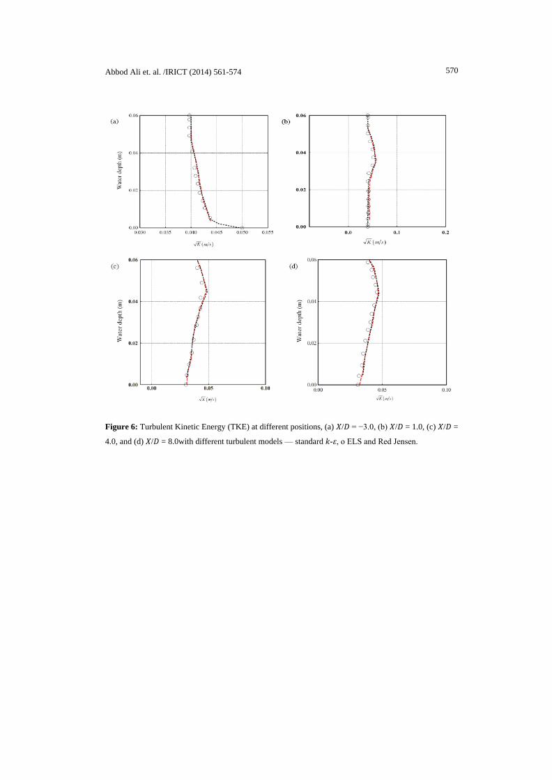
Cases 1-7 are used to predict the horizontal velocity profile (Ux) and the turbulent kinetic

energy (TKE) at some axial length (i.e., X/D= -3.0,1.0,4.0, and 8.0) using different type

turbulence models and the results are presented in Fig.5 and Fig.6 respectively. For

comparisons, the experimental results reported in Jensen et al. [2] are also presented in the

figure. Note that, the location the axial position covers the front and rear part of the pipe (or

obstruction). Referring to Fig.5a tp 5b, which is presented at X/D= -3.0, 1.0, 4.0 and 8.0

respectively, the standard k-ɛ turbulence model prediction is much closer to experimental data

at various water depth; some of them overlap each other. Nearly the same can be said for the

LES model but some deviation seen at some of water depths; for example, at water depths

below 0.03m and those between 0.05 to 0.06 m at X/D = 4.0 (Fig. 5d ). TKE is well predicted

by standard k-ɛ and horizontal velocity profile (Ux) and the turbulent kinetic energy (TKE).

Figure 5: Unsteady horizontal velocity (𝑈𝑥) at different positions, (a) 𝑋/𝐷 = −3.0, (b) 𝑋/𝐷 = 1.0, (c) 𝑋/

㪈 = 4.0, and (d) 𝑋/𝐷 = 8.0with different turbulent models — standard 𝑘-𝜀, ο ELS and Red Jensen.


Figure 6: Turbulent Kinetic Energy (TKE) at different positions, (a) 𝑋/𝐷 = −3.0, (b) 𝑋/𝐷 = 1.0, (c) 𝑋/𝐷 =

4.0, and (d) 𝑋/𝐷 = 8.0with different turbulent models — standard 𝑘-𝜀, ο ELS and Red Jensen.


3.2 Effect of scouring depth

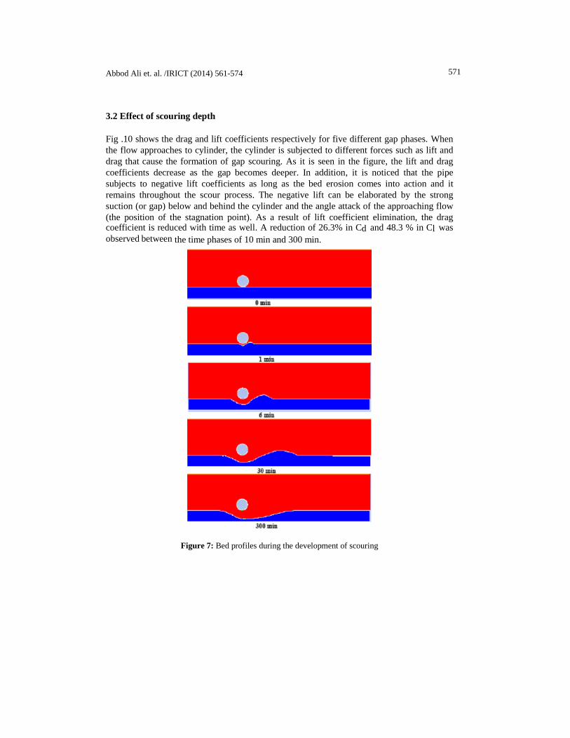
Fig .10 shows the drag and lift coefficients respectively for five different gap phases. When

the flow approaches to cylinder, the cylinder is subjected to different forces such as lift and

drag that cause the formation of gap scouring. As it is seen in the figure, the lift and drag

coefficients decrease as the gap becomes deeper. In addition, it is noticed that the pipe

subjects to negative lift coefficients as long as the bed erosion comes into action and it

remains throughout the scour process. The negative lift can be elaborated by the strong

suction (or gap) below and behind the cylinder and the angle attack of the approaching flow

(the position of the stagnation point). As a result of lift coefficient elimination, the drag coefficient is reduced with time as well. A reduction of 26.3% in Cd and 48.3 % in Cl was

observed between the time phases of 10 min and 300 min.

Figure 7: Bed profiles during the development of scouring


Figure 8: Effect on (a) drag coefficient (𝐶𝑑) and lift coefficient (𝐶𝑙) at cylinder surface of different

time phases.

4. Conclusions and future work

Two dimensional (2D) CFD analyses were carried to investigate fluid flow over an

obstruction under different bed profiles using a number of turbulence models. Unsteady

horizontal velocity profile and the kinetic energy square root at few axial directions are

examined. The effect of scour depth on the drag coefficient, the lift coefficient of the

obstruction body were numerically investigated. The conclusions of the current study are as

follows:

The standard k-ε model and LES both can predict accurate results in comparison to other

turbulence models when compared to experimental data for unsteady horizontal velocity and

turbulent kinetic energy square root but it consumes time and needs a high performance

computer to perform the scouring simulation.

The drag and lift coefficients decrease as the gap under the pipe increases. A reduction of

26.3% in Cd and 48.3% in Cl was observed between the time phases of 10 min and 300 min.

Acknowledgement

The financial support by the high impact research Grants of the University of Malaya

(UM.C/625/1/HIR/61, account no. H-16001-00-D000061) and Exploratory Research Grant

Scheme (ERGS: ER013-2013A) are gratefully acknowledged.

References

1. Breusers, H., G. Nicollet, and H. Shen, Local scour around cylindrical piers.

Journal of hydraulic research, 1977. 15(3): p. 211-252.

2. Chang, H.H., Fluvial processes in river engineering. 1992.

3. 3. Kattell, J. and M. Eriksson, Bridge Scour Evaluation: Screening,


Analysis, & Countermeasures. 1998.

4. Akib, S., Othman, F., Sholichin, M., Fayyadh, M. M., Shirazi, S. Primasari, B.

(2011). Influence of flow shallowness on scour depth at semi-integral bridge piers.

Advanced Materials Research, 243, 4478-4481.

5. Adhikary, B., P. Majumdar, and M. Kostic. CFD Simulation of Open Channel

Flooding Flows and Scouring Around Bridge Structures. in Proceedings of the 6th

WSEAS International Conference on FLUID MECHANICS (FLUIDS’09), L. Xi,

ed. 2009.

6. Shatirah, A., & Budhi, P. (2011). Innovative countermeasure for integral bridge

scour. International Journal of Physical Sciences, 6(21), 4883-4887.‏ 7. Alabi, P.D., Time development of local scour at a bridge pier fitted with a collar.

2006.

8. Shirole, A. and R. Holt, Planning for a comprehensive bridge safety assurance

program. Transportation Research Record, 1991(1290).

9. Guney, M., A. Aksoy, and G. Bombar. Experimental Study of Local Scour Versus

Time Around Circular Bridge Pier. in 6th International Advanced Technologies

Symposium (IATS’11), 16-18 May 2011, Elazığ, Turkey.

10. Akib, S., M. Mohammadhassani, and A. Jahangirzadeh, Application of ANFIS

and LR in prediction of scour depth in bridges. Computers & Fluids, 2014. 91: p.

77-86.

11. Nagata, N., Hosoda, T., Nakato, T., & Muramoto, Y. (2005). Three-dimensional

numerical model for flow and bed deformation around river hydraulic structures.

Journal of hydraulic engineering, 131(12), 1074-1087.‏ 12. Fayyadh, M. M., Akib, S., Othman, I., & Razak, H. A. (2011). Experimental

investigation and finite element modelling of the effects of flow velocities on a

skewed integral bridge. Simulation Modelling Practice and Theory, 19(9), 1795-

181

13. Akib, S., A. Jahangirzadeh, and H. Basser, Local scour around complex pier

groups and combined piles at semi-integral bridge. J. Hydrol. Hydromech, 2014.

62(2): p. 108-116.

14. Akib, S., Jahangirzadeh, A., & Basser, H. (2014). Local scour around complex pier

groups and combined piles at semi-integral bridge. Journal of Hydrology and

Hydromechanics, 62(2), 108-116.

15. Ting, F. C., Briaud, J. L., Chen, H. C., Gudavalli, R., Perugu, S., & Wei, G. (2001).

Flume tests for scour in clay at circular piers. Journal of hydraulic engineering,

‏.969-978 ,(11)12716. Wardhana, K. and F.C. Hadipriono, Analysis of recent bridge failures in the United

States. Journal of Performance of Constructed Facilities, 2003. 17(3): p. 144-150.

17. Murrillo, J.A., The scourge of scour. Civil Engineering—ASCE, 1987. 57(7): p. 66-

69.

18. Briaud, J. L., Ting, F. C., Chen, H. C., Gudavalli, R., Perugu, S., & Wei, G. (1999).

SRICOS: Prediction of scour rate in cohesive soils at bridge piers. Journal of

Geotechnical and Geoenvironmental Engineering, 125(4), 237-246.

19. Akib, S., Othman, I., Othman, F., Fayyadh, M. M., Tunji, L. A. Q., & Shirazi, S. M.

(2011). Epipremnum aureum: An environmental approach to reduce the impact of

integral bridge scour. International Journal of Physical Sciences, 6(27), 6342-6357.

20. Defanti, E., G. Di Pasquale, and D. Poggi. An experimental study of scour at bridge

piers: Collars as a countermeasure. in Proc., 1st IAHR European Congress. 2010.

Heriot-Watt University Edinburgh, UK.

21. Smith, D. Bridge failures. in ICE Proceedings. 1976. Thomas Telford.

22. Mao, Y., The interaction between a pipeline and an erodible bed. SERIES

PAPER TECHNICAL UNIVERSITY OF DENMARK, 1987(39).


23. Jensen, B. L., Sumer, B. M., Jensen, H. R., & Fredsoe, J. (1990). Flow around and

forces.‏ on a pipeline near a scoured bed in steady current. Journal of Offshore

Mechanics and Arctic Engineering, 112(3), 206-213

24. Zhao, M. and L. Cheng, Numerical modeling of local scour below a piggyback

pipeline in currents. Journal of Hydraulic Engineering, 2008. 134(10): p. 1452-

1463.

25. Dudley, R.D., A boroscopic quantitative imaging technique for sheet flow

measurements. 2007, Cornell University.

26. Vass, P., Benocci, C., Rambaud, P., & Lohász, M. M. (2005). Large Eddy

Simulation of a Ribbed Duct Flow with FLUENT: Effect of Rib Inclination.‏ 27. Moeng, C.-H., A large-eddy-simulation model for the study of planetary

boundary-layer turbulence. Journal of the Atmospheric Sciences, 1984. 41(13): p.

2052-2062.

28. Ghosal, S. and P. Moin, The basic equations for the large eddy simulation of

turbulent flows in complex geometry. Journal of Computational Physics, 1995.

118(1): p. 24-37.

29. Kirkil, G., G. Constantinescu, and R. Ettema. The horseshoe vortex system

around a circular bridge pier on equilibrium scoured bed. in World Water and

Environmental Resources Congress, EWRI, Alaska. 2005.

30. Teruzzi, A., Ballio, F., Salon, S., & Armenio, V. (2006). Numerical investigation of

the turbulent flow around a bridge abutment. In L. Cardoso (Ed.), River Flow 2006,

III Int. Conf. on Fluvial Hydraulics, Lisbon, Portugal.‏

31. Fluent, A., Users Guide (nd). , Canonsburg, Pa, USA, 2013.

cfd study of scour gap effect around a pipe - ysrgst.org · 1st international conference of recent...

Documents