CFD SIMULATION OF THE INFLUENCE OF VISCOSITY ON AN

ELECTRICAL SUBMERSIBLE PUMP

A Thesis

by

WENJIE YIN

Submitted to the Office of Graduate and Professional Studies of

Texas A&M University

in partial fulfillment of the requirements for the degree of

MASTER OF SCIENCE

Chair of Committee, Gerald L. Morrison

Committee Members, Michael B. Pate

Karen Vierow

Head of Department, Andreas A. Polycarpou

August 2016

Major Subject: Mechanical Engineering

Copyright 2016 Wenjie Yin

ii

ABSTRACT

Electrical Submersible Pump (ESP) is a multi-stage centrifugal pump used in the

petroleum industry. Due to the high efficiency and adaptivity, ESPs are widely

employed in offshore oil wells. Viscous fluid pumping can result in degradation of ESP

performance. Improving the efficiency and maintaining the performance of ESPs are of

great significance to oil production economic benefit.

To better understand the influence of viscosity on electrical submersible pumps,

this work uses a CFD method to study the flow behaviors inside ESPs. Commercial

software ANSYS Fluent is adopted to simulate the flow field inside the pump. A single

stage of an ESP WJE-1000, manufactured by Baker Hughes Ltd., is modelled and

investigated. 3-D single phase flow numerical simulation is performed to study the pump

performance. Several sets of fluids of different viscosities and densities are tested under

various operation conditions. A wide range of inlet flow rates are calculated for every set

of fluids.

The effects of viscosity on ESP performance is identified and studied thoroughly.

The flow field inside the pump channels is explored by post processing software. To

understand how pump performance changes under different testing conditions,

dimensionless analysis is performed. Shaft power, hydraulic power and drag power are

discussed and calculated by dimensionless numbers.

iii

DEDICATION

To my parents and my lovely Kaimi

iv

ACKNOWLEDGEMENTS

I would like to express my sincere appreciation and thanks to Dr. Gerald

Morrison for his guidance and support on my work. His knowledge, intelligence and

patience helped me to solve various problems throughout the research.

Also, I would like to thank my committee members, Dr. Michael Pate and Dr.

Karen Vierow for their selfless support.

Thanks to Yiming Chen, Abhay Patil and Sujan Reddy for their unconditionally

help on my work.

Thanks also go to all my colleagues at TurboLab, Yi Chen, Changrui Bai, Yintao

Wang, Wenfei Zhang, Peng Liu, Ke Li and Bahadir Basaran, for making my time at

Texas A&M University a great experience.

Finally, thanks to my father and mother for their encouragement and patience

throughout my research.

v

NOMENCLATURE

ESP Electrical Submersible Pump

GVF Gas Volume Fraction

BEP Best Efficiency Point

RMS Root Mean Square

D Diameter

Dh Hydraulic diameter

Ain Inlet cross section area

Ds Length scale of the pump geometries

Q Volumetric flow rate

P Pressure

∆𝑃 Pressure difference

H Head

T Torque

𝑃𝑠ℎ Shaft power

𝑃𝑑𝑟𝑎𝑔 Drag power

𝑁𝑠ℎ Shaft power coefficient

𝑁𝑜𝑢𝑡 Output power coefficient

𝑁𝑑𝑟𝑎𝑔 Drag power coefficient

𝑅𝑒𝐷ℎ Reynolds number based on the hydraulic diameter

𝑅𝑒𝑤 Rotating Reynolds number

g Gravitational acceleration

gpm Gallons per minute

rpm Revolutions per minute

h Blade height

t Blade thickness

vi

Greek Letters

𝜌 Density of the testing fluid

𝜇 Dynamics viscosity

𝑣 Kinematic viscosity

𝜔 Angular speed

𝜂 Pump efficiency

𝛷 Flow rate coefficient

𝛹 Head coefficient

Subscripts

w Value in water cases

v Value in oil cases

1 Impeller inlet

2 Impeller outlet

3 Diffuser inlet

4 Diffuser outlet

i Inner circle

o Outer circle

vii

TABLE OF CONTENTS

Page

ABSTRACT ....................................................................................................................... ii

DEDICATION .................................................................................................................. iii

ACKNOWLEDGEMENTS .............................................................................................. iv

NOMENCLATURE ........................................................................................................... v

TABLE OF CONTENTS ................................................................................................. vii

LIST OF FIGURES ........................................................................................................... ix

LIST OF TABLES ........................................................................................................... xii

I. INTRODUCTION ...................................................................................................... 1

II. LITERATURE REVIEW ........................................................................................... 7

III. OBJECTIVES ........................................................................................................... 11

IV. MODELLING PROCEDURE .................................................................................. 12

IV.1. Electrical Submersible Pump (ESP) .................................................................. 12

IV.2. Model and Mesh ................................................................................................ 16 IV.3. Grid Independence Study .................................................................................. 20

V. SIMULATION SETUP ............................................................................................ 22

V.1. Reynolds Number .............................................................................................. 22

V.2. Solving Model ................................................................................................... 23 V.3. Testing Fluids .................................................................................................... 26 V.4. Boundary Conditions and Time Step ................................................................ 31

VI. RESULTS AND DISCUSSION ............................................................................... 33

VI.1. Pump Performance ............................................................................................ 33 VI.2. Flow Analysis .................................................................................................... 42

viii

VI.3. Performance Analysis ........................................................................................ 48 VI.4. Dimensionless Analysis .................................................................................... 56

VII. CONCLUSIONS ...................................................................................................... 69

REFERENCES ................................................................................................................. 71

APPENDIX A .................................................................................................................. 74

ix

LIST OF FIGURES

Page

Figure I-1: Artificial lift methods illustration [1] ............................................................... 1

Figure I-2: Schematic view of the ESP system [2] ............................................................ 3

Figure I-3: Inner view of the ESP parts [2] ........................................................................ 5

Figure I-4: Comparison of radial-flow impeller and mixed-flow impeller [3] .................. 5

Figure II-1: Head coefficient as a function of flow rate coefficient for oil at various

rotating speeds in centrifugal pumps [8] ......................................................... 8

Figure IV-1: Photo of the impeller of WJE-1000 [15] ..................................................... 12

Figure IV-2: Photo of the diffuser of WJE-1000 [15] ...................................................... 13

Figure IV-3: Dimensions of the impeller of WJE-1000 [15] ........................................... 14

Figure IV-4: Dimensions of the diffuser of WJE-1000 [15] ............................................ 14

Figure IV-5: Catalog performance curve of WJE-1000 at 3600 rpm [15] ....................... 16

Figure IV-6: CAD models of the impeller and the diffuser of WJE-1000 ....................... 17

Figure IV-7: Simplified models of the impeller and the diffuser ..................................... 17

Figure IV-8: Final model of the stage of the pump .......................................................... 18

Figure IV-9: Illustration of the mesh of the whole stage ................................................. 19

Figure IV-10: Comparison of the original mesh and the refined mesh ............................ 20

Figure VI-1: Illustration of the positions of inlet pressure and outlet pressure in the

model ........................................................................................................... 33

Figure VI-2: 2D views of the pressure contour at inlet and outlet of the stage ............... 34

Figure VI-3: Comparison of the pressure rises in psi between the simulation results

and the experimental results for pure water (1cP) [19] .............................. 35

x

Figure VI-4: Modified comparison of the pressure rises in psi between the

simulation results and the experimental results for pure water (1cP) ......... 36

Figure VI-5: Pressure rises for different viscosity oils .................................................... 37

Figure VI-6: Illustration of the positions of the impeller entrance and exit ..................... 38

Figure VI-7: Pressure contour views at the impeller entrance and exit ........................... 39

Figure VI-8: Pressure rises in the impeller for different viscosity oils ............................ 40

Figure VI-9: Pressure differences in the diffuser for different viscosity oils ................... 41

Figure VI-10: Streamlines inside the stage at a flow rate of 437.5 gpm for service

with water (1cP) ......................................................................................... 42

Figure VI-11: Streamlines in the impeller (a) and diffuser (b) at a flow rate of

437.5 gpm for service with water (1cP) ..................................................... 43

Figure VI-12: Streamlines in the impeller (a) and diffuser (b) at a flow rate of

1021 gpm for service with water (1cP) ...................................................... 44

Figure VI-13: Streamlines in the impeller (a) and diffuser (b) at a flow rate of

533 gpm for service with 200cP oil ........................................................... 45

Figure VI-14: Blade-to-blade views of the streamlines in the impeller and diffuser

in (a) Pumping water (1cP) at 583.3 gpm (b) Pumping water (1cP) at

1312 gpm (c) Pumping 200cP oil at 533.6 gpm (d) Pumping 200cP oil

at 1423 gpm ............................................................................................... 47

Figure VI-15: Pressure rises versus viscosities for different flow rates ........................... 49

Figure VI-16: Shaft horsepower for all fluids .................................................................. 50

Figure VI-17: Comparison of the pump efficiencies between simulation results and

experimental results for service with water ............................................... 52

Figure VI-18: Pump efficiency curves for all fluids ........................................................ 53

Figure VI-19: QBEP,V/QBEP versus kinematic viscosity for all fluids ......................... 54

Figure VI-20: H/HBEP,w versus kinematic viscosity for all fluids ................................ 55

Figure VI-21: Head coefficient versus flow rate coefficient for all fluids ....................... 57

xi

Figure VI-22: Pump efficiency versus flow rate coefficient for all fluids ....................... 58

Figure VI-23: Pump efficiency versus flow rate coefficient with trend lines .................. 59

Figure VI-24: Head coefficient versus common logarithm of rotating Reynolds

number and flow rate coefficient in TableCurve 3D ................................. 61

Figure VI-25: Empirical pump performance curve by modified dimensionless

numbers ...................................................................................................... 62

Figure VI-26: Shaft power coefficient versus flow rate coefficient for all fluids ............ 64

Figure VI-27: Output power coefficient versus flow rate coefficient for all fluids ......... 65

Figure VI-28: Drag power coefficient versus flow rate coefficient for all fluids ............ 66

Figure VI-29: Output power coefficient versus head coefficient and flow rate

coefficient in TableCurve 3D .................................................................... 67

Figure VI-30: Drag power coefficient versus head coefficient and flow rate

coefficient in TableCurve 3D .................................................................... 68

xii

LIST OF TABLES

Page

Table IV-1: Dimensions and specifications of WJE-1000 ............................................... 15

Table IV-2: Comparison of the results between the original mesh and the refined

mesh in grid independence study .................................................................. 21

Table V-1: Properties and simulation conditions for pure water ..................................... 27

Table V-2: Properties and simulation conditions for 2.4cP oil ........................................ 27

Table V-3: Properties and simulation conditions for 10cP oil ......................................... 28

Table V-4: Properties and simulation conditions for 60cP oil ......................................... 28

Table V-5: Properties and simulation conditions for 200cP oil ....................................... 29

Table V-6: Properties and simulation conditions for 400cP oil ....................................... 29

Table VI-1: Rotating Reynolds number for all fluids ...................................................... 57

1

I. INTRODUCTION

In the oil field development process, due to the formation energy depleting, the

decreasing pressure head does not allow the reservoir to keep flowing through the wells.

Some reservoirs are originally low in pressure for natural flow. When the production rate

is not satisfactory, artificial lift methods have to be applied.

The commonly used artificial lift methods in the oil and gas industries are shown

in Figure I-1. From left to right are rod pumps, progressing cavity pumps, horizontal

surface pumps, electrical submersible pumps and gas lift. The selection of method

depends on economic, environmental and applicable requirements for different oil wells.

Figure I-1: Artificial lift methods illustration [1]

The rod pump is the most classic artificial lift method in the oil industry. A rod

pump system normally consists of a pump jack, a sucker rod pump and a sucker rod

2

string. The sucker rod string transfers movement and energy from the pump jack on the

ground to the underground sucker rod pump. The sucker rod pump lifts the fluids to the

surface by putting high pressure on the fluids. The equipment for a rod pump system is

inexpensive and reliable, which makes this method the mostly widely used and the most

mature technology among artificial lift methods. The limit of a rod pump system is its

poor performance in lifting high viscous fluids. Progressing cavity pumps have a long

history. Inside a progressing cavity pump, fluids are pushed upwards by the screw blades.

The fluids are lifted by one thread pitch in every rotation cycle. Progressing cavity

pumps have good performance in pumping high viscosity fluids. The disadvantage of

this type of pump is the high maintenance cost as the screws are vulnerable. Horizontal

surface pumps are one type of arrangements of centrifugal pumps. The horizontal

arrangement of surface units is beneficial for installing equipment and maintenance.

Thus horizontal arrangement is often the first choice for economic requirement. The

disadvantage of a horizontal surface pump is its weak applicability under different

working conditions, which leads to limited usage in the offshore oil wells. Gas lift is a

promising artificial lift method in both the downhole and the offshore petroleum

industries. In the gas lift method, high pressure gas (CH4, N2, or CO2) is injected into

the oil wells. The mixture of oil and injected gas has lower density and higher pressure.

Then enough energy is provided for the mixed fluids to flow through the wells. Gas lift

method is versatile and well performed under different geometrical conditions. So

despite of the high initial investment, gas lift is used in a large amount of oil wells.

3

Figure I-2: Schematic view of the ESP system [2]

Electrical submersible pumps are the most commonly employed artificial lift

method in offshore wells. Figure I-2 shows the schematic view of an entire ESP system.

An ESP system consists of subsurface units and surface units. On the ground, there is a

controller, a transformer and a junction box. Located in the well are an electric motor, a

gas separator, a protector and a multistage pump, all work together to lift the oil from the

bottom of the well.

During the lifting procedure, the transformer outputs the required working

voltage from external inlet electricity. The control panel is the central control unit of the

whole system. It provides the underground motor with electric power via flat cables

through the well. When the motor is working, the pump is rotated along with the gas

4

separator. A protector is set around the motor. The protector seals the underground

motor and balances the pressure between the motor and outside environment. The vital

part of the whole system is the subsurface multistage pump. As the fluids enter the pump,

they acquire pressure rise mainly from the impellers inside the pump. After a certain

number of stages, the fluid has enough pressure to flow to the surface. Since the gas in

the mixed fluids will degrade the head of the pump, a gas separator is usually located

below the pump to lower the gas volume fraction (GVF) of the fluids.

The downhole pump is a multistage centrifugal pump. A view of the inner parts

is shown in Figure I-3. As a centrifugal pump, the ESP has impellers and diffusers. The

number of vanes of the impellers and diffusers varies according to the manufacture

design. Commonly, there are five to seven blades in the impeller and similar number of

vanes in the diffuser. A shaft is located in the axial position to transfer movement from

the motor to the rotary parts. At the intake end, bolts are designed for seal. In most ESPs,

the diffusers are stationary; the impellers are rotating along the shaft. When the impeller

rotates about the axis of the pump, the fluids inside the stage are moved outward from

the axis by centrifugal force. With the gained speed and pressure, the fluids flow along

the flow paths and enter the stationary diffuser. The diffuser does not add energy to the

working fluids. It transfers the speed of the fluids into pressure and leads the flow into

next stage while trying to minimize energy loss. As the fluids flow through all impellers

and diffuses, it obtains hydraulic head stage by stage. Eventually, the fluids have enough

pressure to lift itself to the surface.

5

Figure I-3: Inner view of the ESP parts [2]

(a) (b)

Figure I-4: Comparison of radial-flow impeller and mixed-flow impeller [3]

Classified by the impeller design, there are two types of ESP pumps: radial-flow

pumps and mixed-flow pumps. In a radial flow pump, as shown in Figure I-4(a), the

fluids flow into the impeller axially and leave the impeller radially. The pressure rise in

6

this type of impeller is solely contributed by centrifugal force. Although the radial-flow

pump has high hydraulic head, the restriction on flow rate limits its performance and

usage. In a mixed-flow pump, as shown in Figure I-4(b), the fluids leave the impeller in

an angle between axially and radially. The fluids are pushed away by centrifugal force

and impeller shape. The design flow rate of mixed-flow pumps is commonly higher than

radial-flow pumps.

Even considered as a reliable worldwide off shore petroleum production

technology, ESPs have problems facing the complexity of oil fields. Multiphase flow, a

mixture of fluids including gases, will lead to performance degradation. For high gas

volume fraction fluids, free gas gathers at the suction, which lowers the pump efficiency.

The gas may form gas lock which can stop fluid flow under certain conditions. Even in

the simplest single phase flow cases, pumping highly viscous fluids can cause head

degradation. Since the offshore oil field investment is extremely expensive, it is of great

significance to perform researches on the performance of ESPs.

7

II. LITERATURE REVIEW

Karassik [4] introduced the fundamental concepts of centrifugal pumps. The

detail structure of centrifugal pumps was shown and discussed. Performance

characteristics of different types of pumps were comprehensively searched. The head

curve of centrifugal pumps was analyzed to study the performance of centrifugal pumps.

Based on experiments, Ippen [5] used a specified Reynolds number RD to study

centrifugal pump performance. The kinematic viscosity of testing fluid was treated as

one of the determinants of the Reynolds number. Corrections were introduced on head,

power inlet and efficiency. It was concluded that all these parameters could be presented

as a function of the Reynolds number RD. For Reynolds number less than 104 or more

than 106, head correctors tend to be stable. In the analysis, when the Reynolds number is

within the range of 104 to 106, disk and friction loss is thought to be the main reason for

increasing power input. However, the result of the research is not applicable to other

pumps.

Gulich [6], [7] gave a more versatile definition of correction factors of flow rate,

head and efficiency. They are calculated by the following equations.

fQ =Qv

Qw

(II-1)

fH =Hv

Hw

(II-2)

fη =ηv

ηw

(II-3)

8

Some more correction factors were given based on the loss analysis, which

includes the dissipation of the disk friction power. These corrections proved to be useful

when compared with the experimental results of the pumps Gulich tested. In this study,

the first two correction factors will be analyzed to verify the method as a way to study

the effects of viscous fluids on ESPs.

A dimensionless analysis was performed by Timar [8] to study the performance

of centrifugal pumps. Three dimensionless numbers were proposed, which are head

coefficient, flow rate coefficient and the rotating Reynolds number. By the head results

from experiments with a wide range of flow rates for service with water at difference

rotation speed, a universal curve for centrifugal pumps working with water was obtained

in Figure II-1.

Figure II-1: Head coefficient as a function of flow rate coefficient for oil at various

rotating speeds in centrifugal pumps [8]

9

In this figure, the curves for different Reynolds number match perfectly. Also,

the product of flow coefficient and Reynolds number was introduced as another

dimensionless number to study the influence of viscosity.

CFD is a popular method used to study rotational machinery in the last 20 years.

Feng [9] performed CFD simulations on turbulence flow inside a pump to search the

applicability of different models in unsteady flow. The author concluded the turbulence

simulation models can be used to foresee the unsteady flow inside a radial pump. And

there is no significant difference among the turbulence models in pressure related

parameters.

Majidi [10] carried out a 3D flow simulation inside a pump volute. This paper

proved the reliability of CFD codes for solving 3D viscous flow problems inside

centrifugal pumps. Standard k-ε turbulence equation was used for solving the cases in

Majidi’s work.

Barrios [11] performed both single-phase and two-phase flow simulation on

ESPs. As the CFD results were in consistent with experimental results, Barrios was able

to explore numerically the flow field inside the ESP.

Muiltiphase flow inside an ESP is researched numerically by Marsis [12]. High

GVF flow, which is a common problem of ESPs, is studied by CFD simulations in the

research.

A dimensionless method was analyzed on the characteristics of pump

performance. Stel [13] numerically searched the viscosity influences on ESP. Introduced

a new equation to define Reynolds numbers; he discussed the effects of viscosity on

10

head degradation of the pump. Dimensionless numbers were employed in this research.

For cases under different working conditions but the same Reynolds number, it was

revealed that they have the same performance curve and efficiency.

Sirino [14] performed similar simulations with Stel [13] on the same pump. The

flow field inside the pump was investigated. It is found that the streamlines inside the

pump channels are not always bladed oriented.

11

III. OBJECTIVES

When pumping crude oil from offshore wells, high viscosity of the fluids usually

depletes ESP head. To better understand the mechanism of the effects of viscosity on

ESP performance, this research aims to use the CFD method to simulate the complex

flow fields inside ESPs.

In order to lower simulation procedure complexity, simply one of the stages of a

multistage pump is modelled and researched. Balance holes are neglected to reduce the

calculation time and simplify the geometries. The tested ESP model is WJE-1000,

manufactured by Baker Hughes. Gambit is adopted for the meshing task. Commercial

CFD software ANSYS Fluent is used as the CFD solver. Post process and result analysis

are performed in software Teclpot and CFD Post.

Single phase flow is the focus of this work to study the flow behaviors inside the

pump. Transient state simulations should be carried out. The simulation results are to be

compared to experimental results, seeking for good consistency. From the validated CFD

model, flow dynamics in the pump channels can be comprehensively analyzed.

Dimensionless analysis needs to be performed to better understand the performance

characteristics of ESPs. Quantified viscosity related parameters of the performance of

pump need to be found to search the way of improving ESP efficiency. Power related

dimensionless numbers need to be calculated to investigate the performance curve of this

pump.

12

IV. MODELLING PROCEDURE

IV.1. Electrical Submersible Pump (ESP)

The Baker Hughes Centrilift WJE-1000 is the ESP model studied in this work.

This will be referred to as WJE-1000 in the remainder of this thesis. This is a three-stage

centrifugal pump with mixed-flow type impellers. Figure IV-1 shows the suction view of

the impeller. There are five blades in the impeller, along with five balance holes. In the

simulation model, balance holes are removed for simplification.

Figure IV-1: Photo of the impeller of WJE-1000 [15]

13

Figure IV-2: Photo of the diffuser of WJE-1000 [15]

Figure IV-2 shows the discharge view of the diffuser. There are seven vanes in

the diffuser. This is a relatively large pump as the diameter of the stage is 8.15”. The

engineering drawings of the impeller and the diffuser are shown in Figure IV-3 and

Figure IV-4 respectively. The dimensions and specifications of WJE-100 were measured

by the experiment group in the author’s lab.

14

Figure IV-3: Dimensions of the impeller of WJE-1000 [15]

Figure IV-4: Dimensions of the diffuser of WJE-1000 [15]

15

The dimensions and specifications of the impeller and the diffuser are shown in

Table IV-1. Capital letter D denotes to the diameter of a specified surface, while h and t

refers to height and thickness respectively. The subscripts 1, 2, 3 and 4 mean impeller

inlet, impeller outlet, diffuser inlet and diffuser outlet. Inner and outer are differentiated

into subscript i and o.

Table IV-1: Dimensions and specifications of WJE-1000

Dimension Impeller Diffuser

Blades/Vanes 5 blades 7 vanes

Inlet inner diameter (mm) D1,i=48.2 D3,i=183.0

Inlet outer diameter (mm) D1,o=116.5 D3,o=218.6

Inlet blade height (mm) h1=35.0 h3=19.8

Inlet blade hickness (mm) t1=4.8 t3=3.8

Outlet inner diameter (mm) D2,i=183.0 D4,i=48.2

Outlet outer diameter (mm) D2,o=218.6 D4,o=116.5

Outlet blade height (mm) h2=24.8 h4=22.9

Outlet blade thickness (mm) t2=2.1 t4=4.8

16

According to the pump catalog as shown in Figure IV-5, WJE-1000 delivers a

flow rate of nearly 1,100 gallons per minute (gpm) with a pressure rise of 150psi by the

whole three stages at the best efficiency point (BEP) at a rotational speed of 3600 rpm.

Figure IV-5: Catalog performance curve of WJE-1000 at 3600 rpm [15]

IV.2. Model and Mesh

The CAD model of WJE-1000 was acquired by the Turbomachinery Lab. A

single stage including one impeller and one diffuser was investigated in this research.

Figure IV-6 shows the CAD models of the impeller in Figure IV-6(a) and the diffuser in

Figure IV-6(b).

17

(a) (b)

Figure IV-6: CAD models of the impeller and the diffuser of WJE-1000

The geometries of WJE-1000 are too complex to simulate in CFD software.

Simplification on the CAD model was performed to make it possible for calculation. All

five balance holes in the impeller were eliminated to reduce the complexity.

(a) (b)

Figure IV-7: Simplified models of the impeller and the diffuser

18

Figure IV-7 are the views of the simplified models of the impeller and diffuser

respectively. The secondary flow paths were not modelled so to increase the calculation

efficiency. All the seal leakage was not included in this study.

Figure IV-8: Final model of the stage of the pump

Figure IV-8 shows the final model of the whole single stage of WJE-1000 in

Tecplot. The upper side of the model is the inlet of the stage while the bottom is the

discharge of the diffuser. To improve numerical stability for the simulations, a specified

flow rate value was imposed at the inlet of the impeller. The direction of the flow rate is

perpendicular to the face of the inlet. A fixed value reference pressure was set at the

discharge of the diffuser to enhance the calculation quality.

19

All the surfaces in the model were treated as no slip walls. All the clearance, such

as the clearance between the impeller and the diffuser and the gaps around hubs, were

ignored in the model. Software Gambit was employed to perform the meshing task of the

model. In order to reduce the total number of nodes, this thesis used hexahedral elements

rather than tetrahedral elements. Regions such as the blades and the edges were

especially refined for better calculation accuracy. The total number of nodes is 6.76

million for the whole stage, including both the impeller and the diffuser. Then the mesh

was exported to ANSYS Fluent for solving. Figure IV-9 shows the grid of model of

WJE-1000.

Figure IV-9: Illustration of the mesh of the whole stage

20

The structured mesh shows good refinement in critical areas such as the blades

and the hubs. Near wall mesh work was inspected to verify that 𝑦∗ is low enough in

every sub domain.

IV.3. Grid Independence Study

A grid independence study was performed to investigate the influence of number

of nodes on the simulation result. The result of the independence study proves that the

variation in hydraulic head between the original model and the refined model is

negligible.

To study the effect of node numbers, the original grid was more detailed meshed.

The total number of nodes rises to 8.6 million from the primary 6.8 million. Figure

IV-10 (a) shows the original mesh view of the impeller blades and shoulder. Figure

IV-10 (b) shows the refined mesh view of the impeller blades and shoulder. In

comparison, the grid in refined mesh is more detailed in critical parts than the grid in

original mesh. In fact, the mesh in all parts of the stage was refined.

(a) (b)

Figure IV-10: Comparison of the original mesh and the refined mesh

21

The results of both models are concluded in Table IV-2. In the final results, the

area average pressure at the inlet is similar to each other. After the grid refinement, the

pressure rise of the stage changes merely 0.07%. This proves the influence of adding the

number of nodes on the simulation result is negligible. Thus the original grid is

independent of the number of nodes. The original grid was used for all the remaining

CFD simulations as the correct mesh.

Table IV-2: Comparison of the results between the original mesh and the refined mesh

in grid independence study

Original mesh Refined mesh

Number of nodes 6763011 8609436

Pressure outlet (fixed

value) (Pa)

414000 414000

Pressure inlet (Pa) -44960 -45289

Pressure rise (Pa) 458960 459289

Pressure rise (psi) 66.57 66.61

22

V. SIMULATION SETUP

V.1. Reynolds Number

To classify the flow regimes under all operation conditions in this work, the

definition of Reynolds number has to be discussed. There is no literature which provides

a precise methodology in determining Reynolds number for ESPs. Sun [16] presented a

formulation of Reynolds number concerning the cross section shape effect, system

rotation and channel curvature. But the effects of these parameters were studied

separately in simply geometry cases. The combined influence on the modification of

Reynolds number is unknown. And the models studied are not validated with

experimental results in the research. Stel [13] posed a reasonable equation for the

Reynolds number for ESPs. It is based on the inlet cross section area and inlet hydraulic

diameter. This is not a comprehensive methodology because transitional regimes are not

studied in Stel’s work. Although a rough estimation, the results using this equation as the

calculation of Reynolds number shows good consistency with experimental results. The

Reynolds number calculation is Eq. (V-1).

𝑅𝑒𝐷ℎ =(𝑄

𝐴𝑖𝑛⁄ ) ∙ 𝐷ℎ ∙ 𝜌

𝜇 (V-1)

𝑄 is the flow rate of the pump, 𝐴𝑖𝑛 is the inlet cross section area, 𝐷ℎ is the

hydraulic diameter at the inlet, 𝜌 is the density of testing fluid and 𝜇 is the viscosity of

the fluid. In this model, the hydraulic diameter is decided by Eq. (V-2). D1,o is the

impeller outlet diameter and D1,I is the impeller inlet diameter.

23

𝐷ℎ =D1,o -D1,i (V-2)

Based on Stel’s theory [13], cases with Reynolds number larger than 2300 are

treated as being in the turbulence flow regime. Cases with Reynolds number less than

2300 are treated as being in the laminar flow regime.

However, as the definition is rather superficial, some cases with Reynolds

number less than 2300 were still regarded as turbulence flow in this study. In fact, it is

very difficult to infer on the flow regime in the whole stage pump with complex impeller

and diffuser geometries.

V.2. Solving Model

For the turbulence flow, the standard k − ϵ two equations model was utilized in

the Fluent software [17]. This model is based on the Reynolds Averaged Navier-Stokes

Equations (RANS). The transport equations in RANS are shown in Eq. (V-3) and Eq.

(V-4).

The turbulent kinect energy equation for k is calculated as following.

𝜕

𝜕𝑡(𝜌𝑘) +

𝜕

𝜕𝑥𝑖

(𝑝𝑘𝑢𝑖) =𝜕

𝜕𝑥𝑗[(𝜇 +

𝜇𝑡

𝜎𝑘)𝜕𝑘

𝜕𝑥𝑗] + 𝐺𝑘 + 𝐺𝑏 − 𝜌𝜖 − 𝑌𝑀 + 𝑆𝑘 (V-3)

For the dissipation rate 𝜖 is the following equation.

𝜕

𝜕𝑡(𝜌𝜖) +

𝜕

𝜕𝑥𝑖

(𝜌𝜖𝑢𝑖)

=𝜕

𝜕𝑥𝑗[(𝜇 +

𝜇𝑡

𝜎𝜖)

𝜕𝜀

𝜕𝑥𝑗] + 𝐶1𝜖

𝜖

𝑘(𝐺𝑘 + 𝐶3𝜖𝐺𝑏) − 𝐶2𝜖𝜌

𝜖2

𝑘+ 𝑆𝜖

(V-4)

In the equations, 𝐺𝑘 is the turbulence kinect energy generated by the mean

velocity gradient. The equation to calculate 𝐺𝑘 is Eq. (V-5).

24

𝐺𝑘 = −𝜌𝑢𝑖′𝑢𝑗

′̅̅ ̅̅ ̅̅𝜕𝑢𝑗

𝜕𝑥𝑖

(V-5)

Under Boussinesq’s assumption, 𝐺𝑘 is revised as the following definition in

(V-6).

𝐺𝑘 = 𝜇𝑡𝑆2 (V-6)

In the Eq. (V-7), S is the coefficient and defined as.

𝑆 = √2𝑆𝑖𝑗𝑆𝑖𝑗

(V-7)

𝐺𝑏 in the transport equations is the turbulence kinect energy generated by

buoyancy. The equation to calculate 𝐺𝑏 is Eq. (V-8).

𝐺𝑏 = −𝑔𝑖

𝜇𝑡

𝜌𝑃𝑟𝑡

𝜕𝜌

𝜕𝑥𝑖

(V-8)

In the Eq. (V-8), 𝑃𝑟𝑡 is the Prandtl number for turbulence energy and 𝑔𝑖 is the

gravity, and 𝛽 is the coefficient of thermal expansion. The calculation for β is as follows.

𝛽 = −1

𝜌(𝜕𝜌

𝜕𝑇)𝑝

(V-9)

𝑌𝑀 is the dissipation generated from compressible turbulence. In this study, it is

not included. 𝐶1𝜖, 𝐶2𝜖 and 𝐶3𝜖 are model constants. σk and σε are the turbulent Prandtl

numbers for equation k and equation ε. Sk and Sε are user defined source terms.

The turbulence viscosity is decided by k and 𝜖. The equation is as followed.

𝜇𝑡 = 𝜌𝐶𝜇

𝑘2

𝜀

(V-10)

𝐶𝜇 is the model constant.

25

In this study, all the constants are set as Fluent default setting. All these values

are acquainted by experience from practice.

𝐶𝜇 = 0.09 (V-11)

𝐶1𝜀 = 1.44 (V-12)

𝐶2𝜀 = 1.92 (V-13)

𝐶3𝜀 = 1.3 (V-14)

𝜎𝑘 = 1.0 (V-15)

𝜎𝜀 = 1.3 (V-16)

The near wall areas are treated with the standard wall functions in this model.

The equations are based on the assumptions of Launder and Spalading, and employed

widely in flow simulation. The equation for mean velocity area is Eq. (V-17).

𝑈∗ = 1

𝜅𝑙𝑛(𝐸𝑦∗) (V-17)

In this equation, 𝑈∗ and 𝑦∗ are defined as follows.

𝑈∗ = 𝑈𝑃𝐶𝜇

14⁄ 𝑘𝑃

12⁄

𝜏𝑤𝜌⁄

(V-18)

𝑦∗ = 𝜌𝐶𝜇

1/4𝑘𝑃

1/2𝑦𝑃

𝜇

(V-19)

k is the von Karman constant and equals to 0.42 in this model. 𝐸 is the empirical

constant and equals to 9.81. 𝑈𝑃 is the mean velocity of the particle at point P. 𝑘𝑃 is the

turbulence kinect energy at point p. This logarithm is valid for 30 < 𝑦∗ <60. When the

𝑦∗<11.225, the Fluent software uses stress-strain model in which 𝑈∗ = 𝑦∗.

26

For the operating conditions treated as laminar flow, the laminar model was

utilized in Fluent software. The unsteady N-S equations were adopted for laminar flow.

The non-dimensional form of the unsteady incompressible N-S equations is shown as

follows.

𝜕𝜌

𝜕𝑡+ 𝛻 ∙ 𝜌𝑣𝑟⃑⃑ ⃑ = 0 (V-20)

𝜕

𝜕𝑡𝜌𝑣 + 𝛻 ∙ (𝜌𝑣𝑟⃑⃑ ⃑𝑣 ) + 𝜌(�⃑⃑� × 𝑣 ) = −𝛻𝑝 + 𝛻𝜏 + 𝐹

(V-21)

𝜕

𝜕𝑡𝜌𝐸 + 𝛻 ∙ (𝜌𝑣𝑟⃑⃑ ⃑𝐻 + 𝜌𝑢𝑟⃑⃑⃑⃑ ) = 𝛻 ∙ (𝑘𝛻𝑇 + 𝜏 ∙ 𝑣 ) + 𝑆ℎ (V-22)

These are the equations for a rotating frame for absolute velocity in Fluent

software. Eq. (V-20) is the conservation of mass equation. Eq. (V-21) is the conservation

of momentum equation. Eq. (V-22) is the conservation of energy equation.

V.3. Testing Fluids

In order to study the influence of viscosity on the ESP, numerous simulations

under different operation conditions were conducted.

Six groups of different viscosity and density fluids were simulated under seven

various working conditions. The material for the first group is pure water. It is chosen to

validate with the experimental results. Other five groups were conducted by the same oil

of different viscosities. The chosen oil is Conosol C-200 [18]. All working conditions

are summarized in the Table V-1, Table V-2, Table V-3, Table V-4, Table V-5 and

Table V-6.

27

Table V-1: Properties and simulation conditions for pure water

Case Material

Viscosity

(cP)

Density

(kg/m3)

Flow

rate

(gpm)

Reynolds

number

1.1 Water 1 998.2 437.5 212963.9

1.2 Water 1 998.2 583.4 283947.7

1.3 Water 1 998.2 729.1 354884.6

1.4 Water 1 998.2 875.0 425921.6

1.5 Water 1 998.2 1020.9 496908.5

1.6 Water 1 998.2 1166.7 567895.4

1.7 Water 1 998.2 1312.5 638882.4

Table V-2: Properties and simulation conditions for 2.4cP oil

Case Material

Viscosity

(cP)

Density

(kg/m3)

Flow

rate

(gpm)

Reynolds

number

2.1 C-200 2.4 818.4 533.6 88734.9

2.2 C-200 2.4 818.4 711.5 118311.5

2.3 C-200 2.4 818.4 889.3 147868.6

2.4 C-200 2.4 818.4 1067.3 177467.3

2.5 C-200 2.4 818.4 1245.2 207045.2

2.6 C-200 2.4 818.4 1423.0 236623.1

2.7 C-200 2.4 818.4 1600.9 266201.0

28

Table V-3: Properties and simulation conditions for 10cP oil

Case Material

Viscosity

(cP)

Density

(kg/m3)

Flow

rate

(gpm)

Reynolds

number

3.1 C-200 10 818.4 533.6 21296.4

3.2 C-200 10 818.4 711.5 28394.8

3.3 C-200 10 818.4 889.3 35488.4

3.4 C-200 10 818.4 1067.3 42592.2

3.5 C-200 10 818.4 1245.2 49690.8

3.6 C-200 10 818.4 1423.0 56789.5

3.7 C-200 10 818.4 1600.9 63888.2

Table V-4: Properties and simulation conditions for 60cP oil

Case Material

Viscosity

(cP)

Density

(kg/m3)

Flow

rate

(gpm)

Reynolds

number

4.1 C-200 60 818.4 533.6 3549.4

4.2 C-200 60 818.4 711.5 4732.5

4.3 C-200 60 818.4 889.3 5914.7

4.4 C-200 60 818.4 1067.3 7098.7

4.5 C-200 60 818.4 1245.2 8281.8

4.6 C-200 60 818.4 1423.0 9464.9

4.7 C-200 60 818.4 1600.9 10648.0

29

Table V-5: Properties and simulation conditions for 200cP oil

Case Material

Viscosity

(cP)

Density

(kg/m3)

Flow

rate

(gpm)

Reynolds

number

5.1 C-200 200 818.4 533.6 1064.8

5.2 C-200 200 818.4 711.5 1419.7

5.3 C-200 200 818.4 889.3 1774.4

5.4 C-200 200 818.4 1067.3 2129.6

5.5 C-200 200 818.4 1245.2 2484.5

5.6 C-200 200 818.4 1423.0 2839.5

5.7 C-200 200 818.4 1600.9 3194.4

Table V-6: Properties and simulation conditions for 400cP oil

Case Material

Viscosity

(cP)

Density

(kg/m3)

Flow

rate

(gpm)

Reynolds

number

6.1 C-200 400 818.4 533.6 532.

6.2 C-200 400 818.4 711.5 709.9

6.3 C-200 400 818.4 889.3 887.2

6.4 C-200 400 818.4 1067.3 1064.8

6.5 C-200 400 818.4 1245.2 1242.3

6.6 C-200 400 818.4 1423.0 1419.7

6.7 C-200 400 818.4 1600.9 1597.2

30

The properties of pure water are decided by the default values in the material

database of Fluent software, of which viscosity is 0.001 kg/m-s and density is 998.2

kg/m3. The density of C-200 oil is obtained from the manufacture [18]. The change in

density of oil due to the temperature change is neglected in this study. Five different

values of the viscosities of C-200 oil, which are 2.4cP 10cP 60cP 200cP and 400cP,

were chosen among the normal range of viscosity of the oil under ordinary working

conditions. The flow rates for service with water were chosen to follow the experiment

conditions on WJE-1000. Flow rates for service with C-200 oil were chosen accordingly.

During the procedure of experiments, the viscosity of oil will drop dramatically

as the working temperature rises. The change in viscosity will make simulations

extremely difficult. In this study, to better understand the effects of viscosity, all the

values of viscosity of test fluids are set as fixed for simplification. So the impact of

temperature change inside the pump is not included in the results.

The Reynold number is the tables is calculated by the Eq. (V-1). In the equation,

𝑄 is the inlet flow rate as shown in different cases. 𝐴𝑖𝑛 is the cross section area at the

inlet. In the model of WJE-1000, the area is 0.00885 𝑚2 as measured in the chapter 4.

𝐷ℎ is the hydraulic diameter of the inlet. For the stage of the pump, the inlet has an

annulus shape surface. The hydraulic diameter is decided by Eq. (V-2). In this model,

the outer diameter D1,o is 116.6 mm and inner diameter D1,i is 48.2 mm, so the hydraulic

diameter of the model is 68.4 mm in all cases.

Based on literatures, when Reynolds number is larger than 2300, the flow regime

is treated as turbulence. In this research, all the cases with viscosity less than 200cP,

31

were simulated as turbulence flow. In the cases 6.1-6.6, of which fluid viscosity is

400cP, Reynolds numbers are all less than 1600, which were treated as laminar flow.

The difficulty is how to define the flow regimes in 200cP oil cases as the

Reynolds numbers are approaching 2300. In fact, the complexity of the impeller and

diffuser geometries makes it hard to offer a precise method to identify the flow regimes.

Thus in this work, the turbulence model was used in all cases of 200cP oil for the sake of

consistency.

V.4. Boundary Conditions and Time Step

Transient simulations were performed to study the flow behavior inside the

pump. As boundary condition, a specified liquid flow rate was imposed at the inlet of the

stage. A fixed reference pressure of p=100psi was set at the outlet of the stage. Zero psi

was entered as the initial inlet pressure. It is simply a starting value and does not affect

the final flow fields and pressure distribution.

The impeller and inlet inner walls were considered as rotational wall. Diffuser

was regarded as a stationary part. The rotational speed in this study was set as 3600 rpm

according to the pump catalog. All the walls were treated as no-slip walls. In the

impeller flow domain, transient effects were simulated by using moving mesh option.

In all simulations, every time step is set by one degree. Since the rotational speed

is 3600 rpm, the time step size is then 4.62963×10-5 second. In a time step sensibility

test, the time step was set as half degree to study the influence of the time step size,

which is 2.31×10-5 second. For all the performance quantities investigated, discrepancies

32

between the results are less than 1%. The sensibility test proved that the span of

4.62963×10−5 second for time step is reasonable in this pump model.

To achieve the convergence criterion of RMS residual below 10-5, the total

number of time steps was studied. During the calculations, cases with lower viscosity

and lower inlet flow rate tend to be unstable, and need more time steps. With the

sensibility analysis and the proof of simulation tests, all cases need no more than 798

time steps for the inlet pressure to achieve its periodicity.

33

VI. RESULTS AND DISCUSSION

VI.1. Pump Performance

The most important performance quantity of a pump is the pressure rise

(hydraulic head). In this study, the pressure at the outlet of the stage was set as a constant

value of 100psi for reference in all cases. When the simulation reached its periodicity

and the RMS residual went below 10-5, the pressure at the inlet was recorded for

calculation. Figure VI-1(a) shows the position of inlet pressure in the model. Figure

VI-1(b) shows the position of outlet pressure in the model.

(a) (b)

Figure VI-1: Illustration of the positions of inlet pressure and outlet pressure in the

model

34

Figure VI-2(a) is the 2-D view of the pressure contour at the inlet. Figure VI-2(b)

is the pressure contour at the outlet. In Figure VI-2(b), the whole area has the same

pressure at the outlet as it was set to be constant. In Figure VI-2(a), since the pressure at

the inlet is different at various points, the area-weighted average pressure at the inlet

cross section was adopted as the value of the inlet pressure. This method will be used for

the following pressure measurements as well.

(a) (b)

Figure VI-2: 2D views of the pressure contour at inlet and outlet of the stage

Then the pressure rise of the whole stage is calculated as the pressure at the

discharge of the diffuser minus the area-weighted average pressure at the inlet.

35

Figure VI-3: Comparison of the pressure rises in psi between the simulation results and

the experimental results for pure water (1cP) [19]

Figure VI-3 is the comparison for pure water between simulation results and

experimental results. The Y-axis represents the pressure rise of the whole single stage;

and unit is psi. The X-axis is the flow rate in gpm in every case.

The two lines in Figure VI-3 are not the same. There are a couple of reasons for

the deviation.

First of all, all the results for the experiments are the average pressure rise of a

whole three-stage pump. In reality, the pressure rises are not the same in every stage.

Normally, since the inlet flow is strong and unstable, the first stage of the pump has the

lowest hydraulic head. In this CFD model, the flow at the inlet is simulated as normal to

the inlet and is a stable flow field. Thus the hydraulic head of simulations should be

better than the average of multistage experimental results. Due to the lack of data, there

is no correct experimental result of the pressure rise of a single stage.

0

20

40

60

80

100

120

0 500 1000 1500

Pre

ssu

re R

ise

(p

si)

Flow Rate (gpm)

Simulation

Experiment Avearge

36

Secondly, as mentioned above, all five balance holes in the impeller are

neglected in the model. In experiments, due to the reflux and other effects, the balance

holes will contribute to the hydraulic head negatively inside the pump. This might be

main reason for the discrepancy of the two curves in Figure VI-3.

The last but not lease, the leakage and secondary flow are not taken into

consideration in this study. From experiments and literatures, these effects will also

lower the pressure performance of the pump.

Figure VI-4: Modified comparison of the pressure rises in psi between the simulation

results and the experimental results for pure water (1cP)

Due to the lack of data and simplification, a modified comparison between

simulation results and experimental results is given in Figure VI-4. The result of

simulation in every case is reduced by 14 psi which results in the simulations fitting the

0

10

20

30

40

50

60

70

80

90

100

0 500 1000 1500

Pre

ssu

re R

ise

(p

si)

Flow Rate (gpm)

Simulation

Experiment Avearge

37

curve of experimental results. The two curves in Figure VI-4 fit well. In the modified

comparison, better agreement is observed in higher flow rate cases. Deviation is less

than 1.1% for cases at a flow rate of 730 gpm or higher. Largest discrepancy 3.5% is

noted in the case at a flow rate of 437 gpm. As Feng [9] discussed, turbulence models

cannot simulate all flow features in strong part-load conditions. In this way, CFD results

in part-load cases are not as accurate as in over-load cases. Although not a precise

manner, the two fitting curves in Figure VI-4 show good consistency, validating the

model of WJE-1000.

-

Figure VI-5: Pressure rises for different viscosity oils

Figure VI-5 summaries the results of pressure rise for service with different

viscosity oils. In Figure VI-5, one can observe that the head performance is highest in

the lowest flow rate condition for every fluid. As flow rate goes up, the pressure rise

0

10

20

30

40

50

60

70

80

90

0 500 1000 1500 2000

Pre

ssu

re R

ise

(p

si)

FLow Rate (gpm)

2.4cP

10cP

60cP

200cP

400cP

38

declines for every group of oil cases. When the flow rate is increasing, the velocity of

inlet flow is raising as well. The added velocity leads to higher shearing force of the

fluids and higher energy loss. Thus the pressure rise is lower for cases at higher flow

rate. Viscosity of the fluids has the same way of influence on the pump performance.

When pumping highly viscous fluid, the strong shearing force results in more pressure

loss than in low viscous cases. Detailed discussions about the influence of viscosity on

the pump performance are in performance analysis part.

(a) (b)

Figure VI-6: Illustration of the positions of the impeller entrance and exit

39

(a) (b)

Figure VI-7: Pressure contour views at the impeller entrance and exit

The pressure differences in the impeller and diffuser are investigated respectively in

this research. Figure VI-6(a) shows the position of the entrance of the impeller in the

model and Figure VI-6(b) shows the position of the exit of the impeller in the model.

Figure VI-7(a) is the view of pressure contour at the entrance and Figure VI-7(b) is at

the exit. In the impeller, the fluids enter at the exit of the inlet and leave the impeller at

the entrance of the diffuser (the same as the impeller exit). The pressure rise in the

impeller for different viscosity oils is shown in Figure VI-8.

40

Figure VI-8: Pressure rises in the impeller for different viscosity oils

The pressure rise in the impeller is similar to the pressure change of the whole

stage. The difference is that the curves in Figure VI-5 are steeper than the ones in Figure

VI-8. This suggests the performance of the impeller is not as sensitive to flow rate as the

whole stage. A detailed calculation shows the same conclusion regarding the influence

of viscosity. For the whole stage, the pressure rise drops from 56 psi to 30 psi when

replacing 2.4cP oil with 400cP oil at a flow rate of 1100 gpm. In the impeller between

the same two flow rates, the degradation in pressure rise is only 18 psi. The comparison

in viscosity and flow rate change indicates that the performance of the impeller has less

viscosity dependence than the whole stage.

The discrepancy between the hydraulic head of the impeller and the whole stage

is caused by the pressure change inside the diffuser as shown in Figure VI-9. The

entrance of the diffuser is the same as exit of the impeller in Figure VI-6(b) and the exit

0

10

20

30

40

50

60

70

0 500 1000 1500 2000

Pre

ssu

re R

ise

(p

si)

Flow Rate (gpm)

2.4 cP

10cP

60cP

200cP

400cP

41

of the diffuser is the stage outlet as shown in Figure VI-1(b). The curves in Figure VI-9

prove that the diffuser is not always a pressure gain device. Even in pure water cases, the

diffuser contributes to the pressure rise negatively at over-load flow rates. For high

viscosity fluids, the diffuser starts to cause pressure loss in part-load conditions. When

pumping 200cP oil at a flow rate of 1600 gpm, the pressure loss inside the diffuser is

higher than the pressure rise in the impeller, which disables the pump.

Figure VI-9: Pressure differences in the diffuser for different viscosity oils

The pressure change in both the impeller and the diffuser fits well with the head

performance of the whole stage. A little deviation is caused by a small pressure drop in

the inlet of the stage, which is regarded as an independent part of the model.

-40

-30

-20

-10

0

10

20

0 500 1000 1500 2000

Pre

ssu

re D

iffe

ren

ce (

psi

)

Flow Rate (gpm)

2.4 cP

10cP

60cP

200cP

400cP

42

VI.2. Flow Analysis

The flow field in the pump channels was analyzed by the software CFD-Post. An

overall view of the streamlines inside the pump in case 1.1 is shown in Figure VI-10.

Figure VI-10: Streamlines inside the stage at a flow rate of 437.5 gpm for service with

water (1cP)

In this figure, all the blades and hubs are set as transparent to allow visualization

while keeping illustrating the position. All the shrouds are hidden in the same way. The

color scale is a render for local velocity of the fluid.

43

Figure VI-11(a) is the streamlines in the impeller in case 1.1. Figure VI-11(b) is

the streamlines in the diffuser in case 1.1. Large recirculation regions exist in both the

impeller and diffuser in this case.

(a) (b)

Figure VI-11: Streamlines in the impeller (a) and diffuser (b) at a flow rate of

437.5 gpm for service with water (1cP)

When pumping the same fluid, the recirculation zones will reduce at higher flow

rates. Figure VI-12 shows the streamlines in the impeller in Figure VI-12(a) and in the

diffuser in Figure VI-12(b) in case 1.5. This case is chosen as the flow rate is 1021 gpm,

which is close to the BEP. No measurable recirculation regions are found in the impeller.

The recirculation spots in the diffuser become much smaller than in case 1.1.

44

(a) (b)

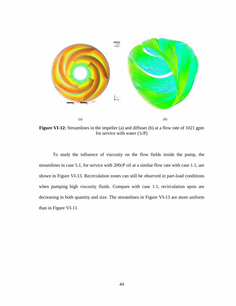
Figure VI-12: Streamlines in the impeller (a) and diffuser (b) at a flow rate of 1021 gpm

for service with water (1cP)

To study the influence of viscosity on the flow fields inside the pump, the

streamlines in case 5.1, for service with 200cP oil at a similar flow rate with case 1.1, are

shown in Figure VI-13. Recirculation zones can still be observed in part-load conditions

when pumping high viscosity fluids. Compare with case 1.1, recirculation spots are

decreasing in both quantity and size. The streamlines in Figure VI-13 are more uniform

than in Figure VI-11.

45

(a) (b)

Figure VI-13: Streamlines in the impeller (a) and diffuser (b) at a flow rate of 533 gpm

for service with 200cP oil

Blade-to-blade views of the streamlines for rotational machinery are shown in

Figure VI-14 Four different operating conditions were selected to study the influence of

viscosity and flow rate. Figure VI-14(a) is the streamlines in case 1.2, representing low

viscosity fluid at part-load flow rate. Figure VI-14(b) is the streamlines in case 1.7,

representing low viscosity fluid at over-load flow rate. Figure VI-14(c) is the streamlines

in case 5.1 representing high viscosity fluid at part-load flow rate. Figure VI-14(d) is the

streamlines in case 5.6, representing high viscosity fluid at over-load flow rate. Blade-to-

blade views of streamlines in the impeller are on the left of each figure, while in the

diffuser are on the right.

In Figure VI-14(a), large recirculation zones occur along the blades in both the

impeller and the diffuser. It shows that when pumping low viscosity fluid at part-load

46

flow rate, large recirculation spots will form along the blades in the impeller and the

diffuser. For service with highly viscous fluid at part-load flow rate, the recirculation

zones are still measurable as seen Figure VI-14(c). The comparison between case 1.1

and case 5.1 indicates that when pumping higher viscosity fluid at part-load flow rate,

the recirculation zones will diminish in both size and quantity. In over-load flow rate

conditions, no recirculation regions are observed for both water and highly viscous oil as

shown in Figure VI-14(b) and Figure VI-14(d).

47

(a) (b)

(c) (d)

Figure VI-14: Blade-to-blade views of the streamlines in the impeller and diffuser in (a)

Pumping water (1cP) at 583.3 gpm (b) Pumping water (1cP) at 1312 gpm (c) Pumping

200cP oil at 533.6 gpm (d) Pumping 200cP oil at 1423 gpm

48

VI.3. Performance Analysis

Figure VI-5 suggests that the pump performance heavily degraded when

pumping highly viscous fluids. In high flow rate cases, the performance recession rate is

even faster as the viscosity rise. According to the pump catalog in Figure IV-5, the pump

stops working at a flow rate of 1750 gpm for service with pure water. This number

decreases to around 1350 gpm when pumping 400cP oil at the same rotational speed

based on Figure VI-5.

To better understand the influence of viscosity on the head performance of the

pump, viscosity is taken as the variable for all the cases. Figure VI-15 shows the curves

of pressure rises versus viscosities for groups of fluids at different flow rates. In this

figure, in lower flow rate cases, the viscosity has less influence on the pressure rise. At a

flow rate of 533 gpm, the performance drop in the pressure rise between 2.4cP oil case

and 400cP oil case is merely 17.5%. By this trend, at the same flow rate, this pump is

able to handle even much higher viscosity fluid with moderate head loss. However, in

the over-load conditions, the pump performance degrades quickly when the viscosity of

the fluid increases. At the flow rate of 1423 gpm, the head decays rapidly from 36psi for

service with 2.4cP oil to -5psi for 400cP oil. The results indicate the viscosity of the

fluids has more influence on the pump performance at higher flow rates.

49

Figure VI-15: Pressure rises versus viscosities for different flow rates

A hydraulic efficiency analysis was performed to study the influence of viscosity

on the pump efficiency and the best efficiency point. Eq. (VI-1) is the calculation for the

pump efficiency

𝜂 =𝜌𝑔𝑄𝐻

𝑇𝜔 (VI-1)

In the equation, 𝜌 is the density of the fluid (kg/m3), 𝑔 is the gravity (m/s2), 𝑄 is

the flow rate (m3/s), 𝐻 is the head (m), 𝜔 is the angular speed (rad/s) and 𝑇 is the torque

(N∙m). 𝑇𝜔 together is the shaft horsepower as shown in Figure VI-16. In the simulations,

𝑇 is the torque provided by all the rotating surfaces in the hydraulic channels. It is

calculated in the software Fluent by integrating the moment to the rotating axis of all

moving internal walls.

-10

0

10

20

30

40

50

60

70

80

90

0 100 200 300 400 500

Pre

ssu

re R

ise

[p

si]

Viscosity [cP]

533 gpm

712 gpm

889 gpm

1067 gpm

1245 gpm

1423 gpm

1601 gpm

50

Theoretically, the numerator in the equation is the product of pressure rise and

flow rate, which represents the output power of the pump. The shaft power in the

denominator may be treated as the input power from the shaft. Efficiency is then defined

as the output power divided by the input power.

Figure VI-16: Shaft horsepower for all fluids

Figure VI-16 summarize the shaft horsepower in every case. At the same flow

rate, the shaft power of the pump does not change considerably when pumping different

viscosity fluids. It can be concluded that viscosity has slight influence on the shaft power

of the pump. The curve for water is higher than all curves for service with oil. The

difference is cause by the density difference between the oil and water. Thus the

40

42

44

46

48

50

52

54

56

58

60

0 500 1000 1500 2000

Shaf

t H

ors

ep

ow

er

(hp

)

Flow Rate (gpm)

Water

2.4cP

10cP

60cP

200cP

400cP

51

efficiency of the pump is mainly decided by the density, flow rate and the product of

hydraulic head and inlet flow rate in every case.

A comparison of the efficiency for service with pure water between the

simulation results and the experimental results is posted in Figure VI-17. As expected,

the efficiency in the simulation cases is higher than in experiment conditions. This is due

internal leakage in the balance holes and the secondary flow paths causing, the

efficiency curve of the experimental results to differ from the simulations and pump

catalog in Figure IV-5. The best efficiency point is different than expected under the

experiment conditions. And the fitting curve is not a smooth one as the curve from

simulation results. Compared with the pump catalog, the efficiencies of simulation

results are slightly higher. As discussed in part 1, the neglect of leakage and energy loss,

the simplification of balance holes and the difference in the number of stages may be the

reasons for the discrepancy of the curves. In simulation results, the best efficiency point

is correct to be the same as the manufacture’s suggestion and the shape of the efficiency

curve from simulation results shows good consistency with the efficiency curve in the

pump catalog in Figure IV-5.

52

Figure VI-17: Comparison of the pump efficiencies between simulation results and

experimental results for service with water

The efficiencies versus flow rates for water and all groups of oils are shown in

Figure VI-18. In low flow rate cases, the pump efficiency degrades consistently due to

the rise of viscosity. At a flow rate of 533.6 gpm, the deviation in efficiencies between

2.4cP oil case and 400cP oil case is 12%. However, at higher flow rates, the pump

efficiency drops dramatically when the fluid viscosity rises. At the best efficiency point

of pure water (1100 gpm), the pump efficiency in 2.4cP oil case is about 33% higher

than the efficiency in 400cP oil case. The efficiency curve for water is not similar to all

oil cases. So the influence of density on pump performance cannot be neglected.

0

0.2

0.4

0.6

0.8

1

0 500 1000 1500

η

Q

Simulationefficiency

Experimentefficiency

53

Figure VI-18: Pump efficiency curves for all fluids

Figure VI-18 proves the best efficiency points are different for various viscosity

fluids at the same rotational speed. For service with pure water, the flow rate at the best

efficiency point is 1100 gpm as shown in Figure IV-5. When pumping 400cP oil, the

flow rate at the best efficiency point decreases to a little over 700 gpm. To better study

the influence of viscosity on the pump efficiency, QBEP,V/QBEP is used as a correction

factor for the flow rate. In the factor, QBEP is the flow rate at the best efficiency point for

service with pure water. QBEP,V is the flow rate at the best efficiency point for service

with any fluid in this study. Since the oil and water in this study have different densities,

kinematic viscosity is employed to be the independent variable in this analysis. Figure

VI-19 shows the QBEP,V/QBEP as a function of the kinematic viscosity for all fluids. The

X-axis is the modification of kinematic viscosity for all fluids.

0

0.1

0.2

0.3

0.4

0.5

0.6

0.7

0.8

0.9

0 500 1000 1500 2000

η

Flow Rate (gpm)

Water

2.4cP

10cP

60cP

200cP

400cP

54

Figure VI-19: QBEP,V/QBEP versus kinematic viscosity for all fluids

This figure clearly demonstrates the change in best efficiency point when

pumping highly viscous oil. By adopting kinematic viscosity, this curve may be used to

predict the best efficiency point for transporting any other fluids. When the kinematic

viscosity of fluid rises, the flow rate has to be lowered to achieve the best efficiency for

the pump. In an ESP, the number of stages has to be added to reach the same head;

meanwhile the production rate of the pump is declining.

Gülich [6],[7] thought the ratio QBEP,V/QBEP is the actual correction factor for the

flow rate. For all the pumps he investigated, the correction factor is still applicable for

points other than the best efficiency point.

0

0.2

0.4

0.6

0.8

1

1.2

0 100 200 300 400 500 600

QB

EP,v

/QB

EP

V*E06 [m2/s]

55

Figure VI-20: H/HBEP,w versus kinematic viscosity for all fluids

A correction factor for the head is studied by the same method as the flow rate in

Figure VI-20. The hydraulic head is normalized by dividing the head for service with

pure water at the best efficiency point in every case. Compared with Figure VI-15, this

chart reveals the influence of viscosity on the pump performance more objectively. The

employment of kinematic viscosity enables the cases for service with pure water to be

added in the figure. For high flow rate cases, the head recession curve is steeper than low

flow rate cases. At a half-load flow rate (533 gpm), the pump performance drops

moderately with the rise in viscosity. This stage of ESP can still provide large percentage

of the original hydraulic head when the viscosity of fluid rises from 1cP to 400cP.

However, at a flow rate of 1423 gpm, the pump performance is quickly degraded when

the viscosity of fluid increases. The curves prove that at higher flow rates, the pump

performance is more sensitive to the viscosity of fluids.

0

0.2

0.4

0.6

0.8

1

1.2

0 100 200 300 400 500 600

H/H

BEP

,W

V*E06 [m2/s]

533 gpm

712 gpm

889 gpm

1067 gpm

1245 gpm

1423 gpm

1601 gpm

56

VI.4. Dimensionless Analysis

A dimensionless analysis was performed by Timar [8] to seek a flow similarity

law for centrifugal pumps working at different rotational speeds. In the same way, this

research used the dimensionless numbers to understand the influence of viscosity on

ESP performance. For the sake of convenience, some of the dimensionless numbers are

modified based on Timar’s work. They are calculated by the following equations.

𝛹 =∆𝑃

𝜌𝐷𝑠2𝜔2

(VI-2)

𝛷 =𝑄

𝜔𝐷𝑠3

(VI-3)

𝑅𝑒𝑤 =𝜌𝜔𝐷𝑠

2

𝜇

(VI-4)

Eq. (VI-2) is the calculation for head coefficient Ψ. Eq. (VI-3) is the definition of

flow rate coefficient Φ; and Eq. (VI-4) represents the rotating Reynolds number 𝑅𝑒𝑤. In

all equations, ∆𝑃 is the pressure rise of the pump (pascal), 𝑄 is the flow rate of the stage

(m3/s), 𝜌 is the density of the fluid (kg/m3), 𝜔 means the angular speed of the impeller

(rad/s), 𝜇 is the dynamics viscosity of the fluid (kg/ms), 𝐷𝑠 is defined as a length scale of

the pump geometries. In this model, 𝐷𝑠 is the impeller outlet mean diameter which is

200.8 mm.

57

Table VI-1: Rotating Reynolds number for all fluids

Fluids 2.4cP 10cP 60cP 200cP 400cP Water

𝑅𝑒𝑤 5139552 1233492 205582.1 61674.62 30837.31 15044870

Figure VI-21: Head coefficient versus flow rate coefficient for all fluids

Table VI-1 summarizes the rotating Reynolds numbers for all testing fluids.

Figure VI-21 is the head coefficient for every group of fluids as a function of flow rate

coefficient. In Figure VI-5, the curves indicate that large head degradation occurs when

pumping highly viscous oil. Similarly, this figure suggests head coefficient is lowered

when rotating Reynolds number is decreased or flow rate coefficient is increased. Solano

[20] concluded that head coefficient 𝛹 should be a function of flow rate coefficient 𝛷

and rotating Reynolds number 𝑅𝑒𝑤 for ESPs.

0

0.02

0.04

0.06

0.08

0.1

0.12

0.14

0 0.01 0.02 0.03 0.04

𝛹

𝛷

(Re)w=15044870

(Re)w=5139552

(Re)w=1233492

(Re)w=205582.1

(Re)w=61674.6

(Re)w=30837.3

58

As expected, the curves in Figure VI-21 are similar with the ones in Figure VI-5.

The benefit to employ these dimensionless numbers is providing a systematic and

mathematic understanding of how pump performance degrades. All the fluid properties

and units have been taken into consideration by nondimensionalization. And similarity

laws can be easily established on the same or similar pump geometries for future

researches working at variable rotational speeds.

A pump efficiency analysis was performed by using dimensionless numbers in

Figure VI-22. This is the same efficiency from Figure VI-18 but now presented as a

function of the flow rate coefficient.

Figure VI-22: Pump efficiency versus flow rate coefficient for all fluids

0

0.1

0.2

0.3

0.4

0.5

0.6

0.7

0.8

0.9

0 0.01 0.02 0.03 0.04

η

𝛷

(Re)w=15044870

(Re)w=5139552

(Re)w=1233492

(Re)w=205582.1

(Re)w=61674.6

(Re)w=30837.3

59

For every curve in Figure VI-22, a multi order polynomial trend line is added to

offer a rough estimation of the performance curves of the pump for service with different

viscosity fluids as shown in Figure VI-23.The starting points of all curves are close to

the origin. For fluids with higher rotating Reynolds number, the flow rate coefficient at

the best efficiency point tends to be larger. The maximum efficiency is lower when

pumping fluids with lower rotating Reynolds number. Based on the figure, the pump

efficiency can be represented as a function of flow rate coefficient 𝛷 and the rotating

Reynolds number 𝑅𝑒𝑤.

Figure VI-23: Pump efficiency versus flow rate coefficient with trend lines

As stated above, head coefficient in every case can be expressed as a function of

flow rate coefficient and rotating Reynolds number. Figure VI-24, created by the

0

0.1

0.2

0.3

0.4

0.5

0.6

0.7

0.8

0.9

0 0.01 0.02 0.03 0.04 0.05

η

𝛷

(Re)w=15044870

(Re)w=5139552

(Re)w=1233492

(Re)w=205582.1

(Re)w=61674.6

60

software TableCurve 3D, plots the points of the three dimensionless numbers for all

cases. The X-axis is flow rate coefficient 𝛷, Y-axis is the common logarithm (logarithm

to base 10) of rotating Reynolds number 𝑅𝑒𝑤 and Z-axis represents the head

coefficient 𝛹. The fitting curved surface, calculated by simple equations, provides a

clear view of the relationship among the three dimensionless numbers for this research.

Since all the points are included, this curved surface may be regarded as a universal

equation to calculate the pump performance. For one stage of this pump, head coefficient

under any working conditions can be determined from the rotating Reynolds number and

flow rate coefficient. Thus, the surface can be used to predict the hydraulic head for

service with any other known fluids with various inlet flow rates. Moreover, affinity

laws can be applied to determine the hydraulic head for cases under different rotational

speeds or in similar pump geometries.

61

Figure VI-24: Head coefficient versus common logarithm of rotating Reynolds number

and flow rate coefficient in TableCurve 3D

A simpler way to acquire a universal solution is to modify the dimensionless

numbers in a 2D chart. Figure VI-25 provides an empirical universal pump performance

curve. The independent variable is set as 𝛷*𝑅𝑒𝑤^-0.066, which is purely an empirical

estimation with no physical meanings. It combines the influence of flow rate coefficient

and Reynolds number. The Y-axis is set as head coefficient. In this figure, the curves of

all groups of cases overlap and approach a universal curve. The new formed curve can

be used as an empirical method to predict the pump performance under different

working conditions.

62

Figure VI-25: Empirical pump performance curve by modified dimensionless numbers

Parameters related to power of the stage are also of importance to the pump

performance. The following equations are the nondimensionlization of shaft power,

output power and drag power.

𝑁𝑠ℎ =𝑃𝑠ℎ

𝜌𝐷𝑠5𝜔3

(VI-5)

𝑁𝑜𝑢𝑡 =𝑄𝐻

𝜌𝐷𝑠5𝜔3

(VI-6)

𝑁𝑑𝑟𝑎𝑔 =𝑃𝑑𝑟𝑎𝑔

𝜌𝐷𝑠5𝜔3

(VI-7)

Eq. (VI-5) is the calculation for shaft power coefficient 𝑁𝑠ℎ. Eq. (VI-6) is the

definition of output power coefficient 𝑁𝑜𝑢𝑡; and Eq. (VI-7) represents the drag power

coefficient𝑁𝑑𝑟𝑎𝑔. In all equations, 𝐻 is the head of the pump (m), 𝑄 is the flow rate of

-0.02

0

0.02

0.04

0.06

0.08

0.1

0.12

0.14

0 0.005 0.01 0.015 0.02

𝛹

𝛷*(𝑅𝑒)𝑤^-0.066

(Re)w=15044870

(Re)w=5139552

(Re)w=1233492

(Re)w=205582.1

(Re)w=61674.6

(Re)w=30837.3

63

the stage (m3/s), 𝜌 is the density of the fluid (kg/m3), 𝜔 means the angular speed of the

impeller (rad/s), 𝐷𝑠 is defined as a length scale of the pump geometries. 𝑃𝑠ℎ is the shaft

power of the pump and 𝑃𝑑𝑟𝑎𝑔 is the drag power of the stage.

The shaft power coefficient 𝑁𝑠ℎ, which represents the power from shaft to the

pump, is an important parameter for pump users. Figure VI-26 is the shaft power

coefficient 𝑁𝑆ℎ versus flow rate coefficient for all cases. The Y-axis has been adjusted to

magnify the difference of the curves. Compared to Figure VI-16, Figure VI-26 is able to

include the curve for water regardless of the difference in density. When the flow rate

coefficient is less than 0.3, the shaft power coefficient is higher in lower Reynolds

number cases. This indicates that under a certain flow rate, the shaft provides more

power for service with higher viscous fluids. When the flow rate coefficient is over 0.3,

shaft power coefficient is lower in lower Reynolds number cases. This may be caused by

the fall in pressure rise when pumping highly viscous fluids at high flow rate.

64

Figure VI-26: Shaft power coefficient versus flow rate coefficient for all fluids

Figure VI-27 is the output power versus flow rate coefficient for every case. In

fact, the output power coefficient, also called hydraulic power, is calculated as the

product of head coefficient and flow rate coefficient. It represents the actual power

absorbed by the output fluid. The curves in Figure VI-27 are identical to the efficiency

curves. For every fluid, there is a maximum output power point which is a function by

the flow rate coefficient and the rotating Reynolds number. Then for service with every

fluid, the pump has a highest output power.

0.0021

0.0022

0.0023

0.0024

0.0025

0.0026

0.0027

0.0028

0 0.01 0.02 0.03 0.04

Nsh

𝛷

(Re)w=15044870

(Re)w=5139552

(Re)w=1233492

(Re)w=205582.1

(Re)w=61674.6

(Re)w=30837.3

65

Figure VI-27: Output power coefficient versus flow rate coefficient for all fluids

Figure VI-28 is drag power coefficient versus flow rate coefficient in every case.

Drag power is the power dissipated in the fluid. It can also be regarded as the wasted

power. The calculation of drag power coefficient is shaft power coefficient minus output

power coefficient. The drag power coefficient for the fluid which has lower rotating

Reynolds number is higher than the fluid which has higher Reynolds number. This trend

indicates that more power is dissipated when pumping more viscous fluid under the

same working condition. Like the output power coefficient curves, the curves in Figure

VI-28 have a lowest point. The points can be chosen as the best working conditions to

minimize the drag power and enhance the efficiency.

-0.0005

0

0.0005

0.001

0.0015

0.002

0.0025

0 0.01 0.02 0.03 0.04

Nout

𝛷

(Re)w=15044870

(Re)w=5139552

(Re)w=1233492

(Re)w=205582.1

(Re)w=61674.6

(Re)w=30837.3

66

Figure VI-28: Drag power coefficient versus flow rate coefficient for all fluids

Figure VI-29: Output power coefficient versus head coefficient and flow rate

coefficient in TableCurve 3D is the output power coefficient versus head coefficient and

flow rate coefficient. Figure VI-30 is the drag power coefficient versus head coefficient

and flow rate coefficient. The curved surface of the plots is a smooth surface and fitted

by simple functions.

0

0.0005

0.001

0.0015

0.002

0.0025

0.003

0.0035

0.004

0 0.01 0.02 0.03 0.04

Ndrag

𝛷

(Re)w=15044870

(Re)w=5139552

(Re)w=1233492

(Re)w=205582.1

(Re)w=61674.6

(Re)w=30837.3

67

Figure VI-29: Output power coefficient versus head coefficient and flow rate coefficient

in TableCurve 3D

68

Figure VI-30: Drag power coefficient versus head coefficient and flow rate coefficient

in TableCurve 3D

For every set of known flow rate coefficient 𝛷 and rotating Reynolds number

𝑅𝑒𝑤, the head coefficient 𝛹 can be obtained from Figure VI-24. As stated above, the

output power coefficient 𝑁𝑜𝑢𝑡 is the product of 𝛷 and 𝛹. The drag power coefficient

𝑁𝑑𝑟𝑎𝑔 may be obtained from Figure VI-30. Then the shaft power coefficient 𝑁𝑠ℎ can be

calculated as 𝑁𝑜𝑢𝑡+𝑁𝑑𝑟𝑎𝑔. So under every condition, all three power coefficients can be

calculated from Figure VI-24 and Figure VI-30.

All the dimensionless numbers are meaningful for pump users. The

dimensionless numbers provide a systematic and mathematic relation of the pump

performance.

69

VII. CONCLUSIONS

In this research, a CFD method was adopted to investigate the flow behavior and

pressure performance of one stage of an Electrical Submersible Pump. The influence of

viscosity on the pump performance was studied throughout the analysis.

Compared with the pump catalog and experimental results, the simulation results

show good consistency and validate the model of the pump. Head degradation due to the

use of high viscosity fluids is clearly illustrated by plotting the pressure rise of the pump

in every case. Pressure change in the impeller and the diffuser are studied separately. It

was revealed that when pumping highly viscous fluids at high flow rate, the diffuser can

cause pressure lose rather than provide positive hydraulic head.

Four different cases were chosen to investigate the flow behavior inside the

pump channels. For low viscosity fluid in part-load conditions, large recirculation

regions are observed along the blades in the impeller and the diffuser. When pumping

high viscosity fluid at the same part-load flow rate, recirculation regions decrease in both

quantity and size. For over-load flow rate conditions, no recirculation zones are found

for both low viscosity fluid and high viscosity fluid.

It is proven that the pump performance is more sensitive to the rise of viscosity at

higher flow rates than lower flow rates. In this research, an analysis of the pump

efficiency is performed. The maximum efficiency is lowered for service with higher

viscosity fluid. Moreover, the flow rate at the best efficiency point is descending as the

viscosity of fluid increases. Thus, to keep the pump working at the best efficiency point

70

for service with higher viscosity fluids, flow rate (which is also the production rate)

needs to be decreased, while the number of stages must be added in order to maintain the

hydraulic head of the whole pump.

Dimensionless numbers are introduced to better understand the influence of

viscosity on pump performance. It is concluded that head coefficient and the pump

efficiency can be represented as functions of flow rate coefficient and rotating Reynolds

number. A 3D curved surface is calculated based on all cases as a universal solution. The

surface can be used to predict the pump performance under various working conditions.

Power coefficients are discussed. Output power coefficient is directly obtained

from head coefficient and flow rate coefficient. The drag power coefficient which is

caused by viscosity proved to be a function of head coefficient and flow rate coefficient.

Then the shaft power coefficient can be obtained from these two power coefficients.

For the future work, the recommendation is to investigate the pump performance

at different rotational speeds. As the dimensionless numbers are adopted, affinity laws

can be used to predict the pump performance at various rotational speeds.

71

REFERENCES

[1] Schlumberger. “Pushing Up the Range of Options.” 2015; Available from:

http://www.slb.com/~/media/Files/artificial_lift/industry_articles/201503-

upstream-tech-pushing-up-range-of-options.pdf.

[2] Baker Hughes. “ESP System Technology Overview.” 2013.

[3] ESDU, Radial mixed and axial flow pumps. Introduction. ESDU Series on Fluid

Mechanics. 1980: ESDU. 61.

[4] Karassik, I.J. and J.T. McGuire, Centrifugal pumps. 2nd ed. 1998: New York :

Chapman & Hall : International Thomson, 1998 2nd ed.

[5] Ippen, A. T., 1945, “The influence of viscosity on centrifugal pump performance,”

Issue 199 of Fritz Engineering Laboratory report, ASME Paper No. A-45-57

[6] Gülich, J.f., 1999, "Pumping Highly Viscous Fluids with Centrifugal Pumps —

Part 1." World Pumps 1999(395): p. 30-34.

[7] Gülich, J.f., 1999, "Pumping Highly Viscous Fluids with Centrifugal Pumps —

Part 2." World Pumps 1999(396): p. 39-42.

[8] Timar, P., “Dimensionless Characteristics of Centrifugal Pump.” Chemical

Papers- Slovak Academy of Sciences, 2005. 59: p. 500-503.

[9] Feng, J., F.K. Benra, and H. Dohmen, “Application of Different Turbulence

Models in Unsteady Flow Simulations of a Radial Diffuser Pump.” Anwendung

verschiedener Turbulenzmodelle zur Simulation der transienten Strömung in einer

Radialpumpe mit beschaufeltem Diffusor. 2010. 74(3): p. 123.

72

[10] Majidi, K. and H.E. Siekmann, “Numerical Calculation of Secondary Flow in

Pump Volute and Circular Casings using 3D Viscous Flow Techniques.”

International Journal of Rotating Machinery, 2000. 6(4): p. 245.

[11] Barrios, L.J., “Visualization and Modeling of Multiphase Performance inside an

Electrical Submersible Pump”. 2007: (PHD Thesis, The University of Tulsa).

[12] Rasmy Marsis, E.G. and G. Morrison, “CFD Simulation and Experimental

Testing of Multiphase Flow Inside the MVP Electrical Submersible Pump”. 2013:

(PHD Thesis, Texas A & M University).

[13] Stel, H., Sirino T., P.R.Pamella., “CFD Investigation of the Effect of Viscosity on

a Three-Stage Electric Submersible Pump.” In ASME 2014 4th Joint US-

European Fluids Engineering Division Summer Meeting collocated with the

ASME 2014 12th International Conference on Nanochannels, Microchannels, and

Minichannels. 2014. American Society of Mechanical Engineers.

[14] Sirino T., Stel,H., “Numerical study of the influence of viscosity on the

performance of an Electric Submersible Pump”. In ASME 2013 Fluids

Engineering Division Summer Meeting 2013. American Society of Mechanical

Engineers.

[15] Carvajal Diaz, N.I. and G. Morrison, “Effects of Sand on the Components and

Performance of Electric Submersible Pumps.” 2013: (MS Thesis, Texas A & M

University).

[16] Sun, D. and M.G. Prado, “Single-Phase Model for Electric Submersible Pump

(ESP) Head Performance”. SPE Journal, 2006. 11(01): p. 80-88.

73

[17] Fluent, A., Ansys Fluent theory guide. ANSYS Inc., USA, 2011.

[18] Calumet Speciaty Products Parteners, L.P. “Conosol Products.” 2008; Available

from:http://www.calumetsolvents.com/images/spec-

sheets/Oil_Drilling_Conosols_2-12.pdf.

[19] Sujan Reddy and G. Morrison, “Experimental Results of an Electric Submersible

Pump WJE-1000”. 2016, Texas A & M University.

[20] Solano, E.A., “Viscous Effects on the Performance of Electro Submersible Pumps

(ESP's)”. 2009: (MS Thesis, The University of Tulsa).

74

APPENDIX A

Table A-1: Pressure rise for three stages for service with water from experimental

results

Liquid Flow Rate

(GPM)

Pressure Rise(psi) Liquid Flow Rate

(GPM)

Pressure Rise(psi)

1245.454492 150.9168723 843.9751672 210.585432

1201.899912 164.726172 802.76351 215.3792913

1149.460445 171.8517462 751.5724593 220.9897089

1113.994854 179.2126045 698.2985364 227.1165952

1050.350146 187.6568339 623.8918205 236.0475731

1001.08742 194.3274047 607.1648746 238.1256344

954.0869712 198.1714808 551.470833 245.3765626

Table A-2: Pressure difference for the stage for all oils in psi

Flow Rate

(gpm)

2.4cP 10cP 60cP 200cP 400cP

533.6437114 79.98 77.52 73.748122 69.39 65.05

711.5146182 71.13 68.67 65.19088 61.13 55.76

889.2677584 65.05 62.14 57.93898 50.83 43.87

1067.271927 58.08 53.39 46.33594 37.92 29.37

1245.150582 48.37 42.42 32.702368 21.82 11.38

1423.029236 35.75 28.35 15.732922 2.53 -10.373918

1600.907891 20.37 11.53 -4.42736 -20.526578 -35.755568

75

Table A-3: Pump efficiency for all fluids

Case Series 2.4cP 10cP 60cP 200cP 400cP Water

Case 1 0.491194 0.474428 0.448228 0.417825 0.383837 0.50923

Case 2 0.566434 0.53705 0.496285 0.453776 0.402733 0.637925

Case 3 0.601953 0.568313 0.518634 0.443918 0.372463 0.708707

Case 4 0.616629 0.563492 0.477827 0.383619 0.290173 0.750268

Case 5 0.591571 0.517148 0.393095 0.258817 0.13309 0.785291

Case 6 0.510863 0.407753 0.225005 0.036084 0.783426

Case 7 0.3472 0.199945 0.746831

Table A-4: Shaft horsepower in all cases in hp

Case

Series

2.4cP 10cP 60cP 200cP 400cP Water

Case 1 41.25464 41.39586 41.6841 42.07892 42.93298 50.47283

Case 2 42.42283 43.19307 44.37177 45.50537 46.77169 50.41746

Case 3 45.62008 46.16558 47.16389 48.34317 49.72644 52.2267

Case 4 47.72817 48.18595 49.13484 50.09016 51.27873 55.38859

Case 5 48.33105 48.48901 49.178 49.84721 50.55373 57.80759

Case 6 47.27485 46.97373 47.23869 47.45202 47.5425 59.21902

Case 7 44.59979 43.81598 43.37746 42.96328 42.37737 59.40609

76

Table A-5: Pressure drop in the inlet for all oils in psi

Flow Rate

(gpm)

2.4cP 10cP 60cP 200cP 400cP

533.6437114 0.72519 0.580152 0.72519 0.870228 1.160304

711.5146182 1.015266 2.17557 1.305342 1.45038 1.595418

889.2677584 1.305342 1.305342 0.870228 2.030532 2.320608

1067.271927 1.740456 2.030532 2.320608 2.755722 3.045798

1245.150582 2.17557 2.610684 2.90076 3.62595 4.061064

1423.029236 2.755722 3.190836 3.770988 4.496178 5.221368

1600.907891 3.480912 4.061064 4.786254 5.511444 6.381672

Table A-6: Pressure rise in the impeller for all oils in psi

Flow Rate

(gpm)

2.4 cP 10cP 60cP 200cP 400cP

533.6437114 63.96176 62.65642 61.061 59.03047 56.8549

711.5146182 61.061 60.91596 57.87016 55.54955 52.79383

889.2677584 58.59535 56.56482 53.8091 50.32819 46.41216

1067.271927 54.53429 51.63353 47.86254 43.65644 38.87018

1245.150582 49.31292 45.68697 40.61064 35.53431 29.87783

1423.029236 43.22132 37.99996 32.0534 25.9618 19.29005

1600.907891 36.2595 30.1679 22.33585 14.64884 6.961824

77

Table A-7: Pressure change in the diffuser for all oils in psi

Flow Rate

(gpm)

2.4 cP 10cP 60cP 200cP 400cP

533.6437114 16.74819 15.44285 13.41231 11.23674 9.35125

711.5146182 11.09171 9.931402 8.62606 7.030642 4.564996

889.2677584 7.755832 6.885604 5.00011 2.534464 -0.22126

1067.271927 5.290186 3.984844 0.794008 -2.97698 -6.45789

1245.150582 1.229122 -0.65637 -5.00751 -10.0838 -14.435

1423.029236 -4.71744 -6.45789 -12.5495 -18.9312 -24.4426

1600.907891 -12.4045 -14.58 -21.977 -29.664 -36.3357

Table A-8: Kinematic viscosity in all cases

V*E06

(m2/s)

2.4cP 10cP 60cP 200cP 400cP Water

Case 1 2.932551 12.21896 73.31378 244.3793 488.7586 1.001803

Case 2 2.932551 12.21896 73.31378 244.3793 488.7586 1.001803

Case 3 2.932551 12.21896 73.31378 244.3793 488.7586 1.001803

Case 4 2.932551 12.21896 73.31378 244.3793 488.7586 1.001803

Case 5 2.932551 12.21896 73.31378 244.3793 488.7586 1.001803

Case 6 2.932551 12.21896 73.31378 244.3793 488.7586 1.001803

Case 7 2.932551 12.21896 73.31378 244.3793 488.7586 1.001803

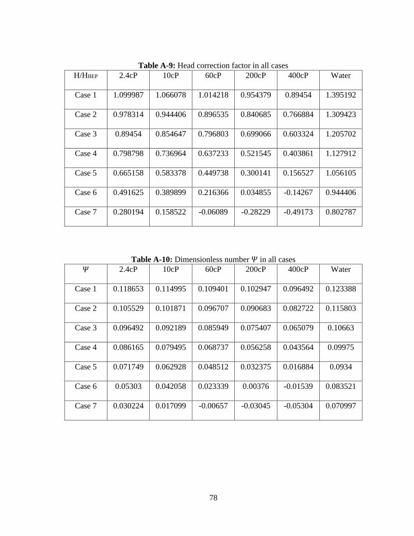
78

Table A-9: Head correction factor in all cases

H/HBEP 2.4cP 10cP 60cP 200cP 400cP Water

Case 1 1.099987 1.066078 1.014218 0.954379 0.89454 1.395192

Case 2 0.978314 0.944406 0.896535 0.840685 0.766884 1.309423

Case 3 0.89454 0.854647 0.796803 0.699066 0.603324 1.205702

Case 4 0.798798 0.736964 0.637233 0.521545 0.403861 1.127912

Case 5 0.665158 0.583378 0.449738 0.300141 0.156527 1.056105

Case 6 0.491625 0.389899 0.216366 0.034855 -0.14267 0.944406

Case 7 0.280194 0.158522 -0.06089 -0.28229 -0.49173 0.802787

Table A-10: Dimensionless number 𝛹 in all cases

𝛹 2.4cP 10cP 60cP 200cP 400cP Water

Case 1 0.118653 0.114995 0.109401 0.102947 0.096492 0.123388

Case 2 0.105529 0.101871 0.096707 0.090683 0.082722 0.115803

Case 3 0.096492 0.092189 0.085949 0.075407 0.065079 0.10663

Case 4 0.086165 0.079495 0.068737 0.056258 0.043564 0.09975

Case 5 0.071749 0.062928 0.048512 0.032375 0.016884 0.0934

Case 6 0.05303 0.042058 0.023339 0.00376 -0.01539 0.083521

Case 7 0.030224 0.017099 -0.00657 -0.03045 -0.05304 0.070997

79

Table A-11: Dimensionless number 𝛷 in all case

𝛷 2.4cP 10cP 60cP 200cP 400cP Water

Case 1 0.011169 0.011169 0.011169 0.011169 0.011169 0.009157

Case 2 0.014892 0.014892 0.014892 0.014892 0.014892 0.012209

Case 3 0.018612 0.018612 0.018612 0.018612 0.018612 0.01526

Case 4 0.022338 0.022338 0.022338 0.022338 0.022338 0.018314

Case 5 0.026061 0.026061 0.026061 0.026061 0.026061 0.021366

Case 6 0.029783 0.029783 0.029783 0.029783 0.029783 0.024419

Case 7 0.033506 0.033506 0.033506 0.033506 0.033506 0.027471

Table A-12: Dimensionless number 𝑁𝑠ℎ in all cases

𝑁𝑠ℎ 2.4cP 10cP 60cP 200cP 400cP Water

Case 1 0.002197 0.002204 0.00222 0.002241 0.002286 0.002203

Case 2 0.002259 0.0023 0.002363 0.002423 0.00249 0.002201

Case 3 0.002429 0.002458 0.002511 0.002574 0.002648 0.00228

Case 4 0.002541 0.002566 0.002616 0.002667 0.00273 0.002418

Case 5 0.002573 0.002582 0.002619 0.002654 0.002692 0.002524

Case 6 0.002517 0.002501 0.002515 0.002527 0.002531 0.002585

Case 7 0.002375 0.002333 0.00231 0.002288 0.002256 0.002593

80

Table A-13: Dimensionless number 𝑁𝑜𝑢𝑡 in all cases

𝑁𝑜𝑢𝑡 2.4cP 10cP 60cP 200cP 400cP Water

Case 1 0.001325 0.001272 0.001218 0.00115 0.00108 0.00113

Case 2 0.001572 0.001513 0.001434 0.001339 0.001228 0.001414

Case 3 0.001796 0.001716 0.0016 0.0014 0.001267 0.001627

Case 4 0.001925 0.001776 0.001535 0.001257 0.001084 0.001827

Case 5 0.00187 0.001651 0.001276 0.000858 0.000599 0.001996

Case 6 0.001579 0.001264 0.000695 0.000112 -0.00023 0.002039

Case 7 0.001013 0.000591 -0.00018 -0.00099 -0.00147 0.00195

Table A-14: Dimensionless number 𝑁𝑑𝑟𝑎𝑔 in all cases

𝑁𝑑𝑟𝑎𝑔 2.4cP 10cP 60cP 200cP 400cP Water

Case 1 0.000871 0.000931 0.001001 0.00109 0.001205 0.001073

Case 2 0.000686 0.000786 0.000928 0.001083 0.001261 0.000786

Case 3 0.000632 0.000741 0.000911 0.001173 0.001379 0.000652

Case 4 0.000616 0.000789 0.00108 0.001409 0.001646 0.00059

Case 5 0.000703 0.00093 0.001342 0.001795 0.002092 0.000527

Case 6 0.000937 0.001237 0.001819 0.002414 0.00276 0.000545

Case 7 0.001361 0.001741 0.002488 0.003281 0.003722 0.000642