cfd simulation of jet cooling and implementation of flow

CFD Simulation of Jet Cooling and

Implementation of Flow Solvers in GPU

M D. L O K M A N H O S A I N

Master of Science Thesis Stockholm, Sweden 2013

CFD Simulation of Jet Cooling and Implementation of Flow Solvers in GPU

M D . L O K M A N H O S A I N

Master’s Thesis in Scientific Computing (30 ECTS credits) Master Programme in Scientific Computing 120 credits Royal Institute of Technology year 2013

Supervisor at ABB was Rebei-Bel Fdhila Supervisor at KTH was Jesper Oppelstrup Examiner was Michael Hanke TRITA-MAT-E 2013:30 ISRN-KTH/MAT/E--13/30--SE Royal Institute of Technology School of Engineering Sciences KTH SCI SE-100 44 Stockholm, Sweden URL: www.kth.se/sci

AbstractIn rolling of steel into thin sheets the final step is the cooling of thefinished product on the Runout Table. In this thesis, the heat transferinto a water jet impinging on a hot flat steel plate was studied as the keycooling process on the runout table. The temperature of the plate waskept under the boiling point. Heat transfer due to a single axisymmet-ric jet with different water flow rate was compared to cases of a singlejet and two jets in 3D. The RANS model in ANSYS Fluent was usedwith the k− ε model in transient simulation of the axisymmetric modeland steady flow for the 3D cases. Two different boundary conditions,constant temperature and constant heat flux were applied at the sur-face of the steel plate. The numerical results were consistent between2D and 3D and compared well to literature data. The time dependentsimulations for the 3D model requires very large computational powerwhich motivated an investigation of simpler flow solvers running on aGPU platform. A simple 2D Navier-Stokes solver based on Finite Vol-ume Method was written using OpenCL which can simulate flow andheat convection. A standard CFD problem named "Lid Driven Cavity"in 2D was chosen as validation case and for performance measurementand tuning of the solver.

ReferatCFD-simulering av kylning med vattenstrålar och

GPU-implementering av strömningslösareNär stål valsas till plåt är det sista steget att kyla den färdiga produk-ten på utrullningsbordet (ROT). I detta arbete studeras värmetrans-porten i en vattenstråle som faller in mot en varm plan platta somär den viktigaste kylprocessen på utrullningsbordet. Plattans temper-atur hölls under kokpunkten. Värmeövergång i en ensam rotationssym-metrisk stråle med olika hastighet jämförs med en och två strålar i3D modeller. RANS-modellering i ANSYS Fluent med k − ε turbulens-modell används för transientberäkning för rotationssymmetri och förstationär beräkning för 3D-fallen. Två olika randvillkor, konstant tem-peratur och konstant värmeflöde, används vid plattan. De numeriskaresultaten är konsistenta mellan rotationssymmetri och 3D och jämför-bara med litteratur-data.

Transient simulering av 3D modellerna kräver stora datorresurser vilketmotiverar en undersökning om enklare strömninngsmodeller som kanköra på GPU-plattform. En enkel 2D Navier-Stokes-lösare baserad påFinita Volym-metoden implementerades i OpenCL för simulering avkonvektiv värmetransport. Lid Driven Cavity-problemet i 2D valdes förverifiering och tidtagning.

Acknowledgements

I would like to acknowledge the invaluable guidance, encouragement and advicefrom my supervisor Prof. Jesper Oppelstrup throughout this thesis work. Thisthesis would not have been possible without his support. So my first and foremostthanks goes to him.

This dissertation is done at ABB. So, I would like to express my gratitude to mysupervisor Rebei Bel-Fdhila at ABB for his constant support and assistance inthis master thesis work. I am also grateful to ABB and Anders Daneryd, projectmanager at ABB for giving me this opportunity.

My special thanks goes to Davoud Saffar Shamshirgar, Ph.D student at NA group,KTH for his advice and discussion about GPU programming. I thank Reza Fakhraieand Bahram Saadatfar from Energy Department at KTH for their constructivediscussion on GPU.

Finally, I would like to acknowledge the Computational Fluid Dynamics course atMechanics department at KTH for the Matlab template of a 2D Navier-Stokes solverwhich helped me a lot to implement the solver on GPU.

Contents

List of Figures

1 Introduction 1

2 Physical and Theoretical Background 32.1 Physics of Impinging Jet . . . . . . . . . . . . . . . . . . . . . . . . . 32.2 Governing Equations . . . . . . . . . . . . . . . . . . . . . . . . . . . 4

3 Literature Review 9

4 Computational domain and Mesh 13

5 Results and Discussion 175.1 2D- Axisymmetric model . . . . . . . . . . . . . . . . . . . . . . . . 185.2 3D 1-jet model . . . . . . . . . . . . . . . . . . . . . . . . . . . . . . 245.3 3D 2-jet model . . . . . . . . . . . . . . . . . . . . . . . . . . . . . . 24

6 GPGPU 296.1 Different Methods . . . . . . . . . . . . . . . . . . . . . . . . . . . . 306.2 Why OpenCL? . . . . . . . . . . . . . . . . . . . . . . . . . . . . . . 31

6.2.1 OpenCL basics . . . . . . . . . . . . . . . . . . . . . . . . . . 316.3 Algorithm and Implementation . . . . . . . . . . . . . . . . . . . . . 346.4 Results and Performance . . . . . . . . . . . . . . . . . . . . . . . . . 35

6.4.1 Speedup . . . . . . . . . . . . . . . . . . . . . . . . . . . . . . 366.4.2 Profiling and Debugging . . . . . . . . . . . . . . . . . . . . . 376.4.3 Optimization techniques . . . . . . . . . . . . . . . . . . . . . 38

7 Conclusion and Future Work 45

Bibliography 47

List of Figures

1.1 Hot rolling steel mill and the Runout table process [14] . . . . . . . . . 2

2.1 Typical Axisymmetric jet configuration . . . . . . . . . . . . . . . . . . 42.2 Different zone of an axisymmetric impinging jet . . . . . . . . . . . . . . 52.3 Visualization of hydraulic jump(picture taken from a sink at home) . . . 6

4.1 Geometry of the 2D-Axisymmetric Case . . . . . . . . . . . . . . . . . . . . 134.2 Mesh of the 2D-Axisymmetric Case . . . . . . . . . . . . . . . . . . . . . . 144.3 Geometry for the 3D 1-jet model . . . . . . . . . . . . . . . . . . . . . . . . 144.4 Geometry for the 3D 2-jet model . . . . . . . . . . . . . . . . . . . . . . 154.5 Full mesh for the 3D 1-jet model . . . . . . . . . . . . . . . . . . . . . . . . 154.6 Zoomed mesh for the 3D 1-jet model . . . . . . . . . . . . . . . . . . . . 16

5.1 Velocity vector plot of the stagnation zone . . . . . . . . . . . . . . . . . . . 185.2 Interface shape for different water velocity at inlet . . . . . . . . . . . . . . . 195.3 Volume Fraction of water liquid for two different water flow rate . . . . 205.4 Water film thickness comparison . . . . . . . . . . . . . . . . . . . . . . . . 215.5 Comparison of nusselt numbet at the stagnation point with theory . . . . . . 225.6 Comparison of Nusselt number with theory upto 5 diameter from impinging point 235.7 Nusselt Number for different water speed at inlet . . . . . . . . . . . . . . . 245.8 Nusselt number comparison between different boundary conditions . . . . . . 255.9 Nusselt Number comparison between 2D and 3D models . . . . . . . . . . . . 255.10 Interface comparison between 2D and 3D models . . . . . . . . . . . . . . . 265.11 Volume of fluid for the 2-jet simulation in 3D shows the splashing at YZ sym-

metry plane which occurs due to the collision of two waves from two jets . . . 27

6.1 A typical GPU platform architecture . . . . . . . . . . . . . . . . . . . . . . 326.2 Index space for NDRange [20] . . . . . . . . . . . . . . . . . . . . . . . . . 336.3 OpenCL memory hierarchies [20] . . . . . . . . . . . . . . . . . . . . . . . 346.4 Sample output from GPU program . . . . . . . . . . . . . . . . . . . . . 376.5 Speedup for different problem size . . . . . . . . . . . . . . . . . . . . . 376.6 Time taken by each kernel in one time step . . . . . . . . . . . . . . . . . . 386.7 GPU time summary plot which shows the total running and idle time . . . . . 396.8 Idle time of GPU device (snap of one iteration of CG algorithm) . . . . . . . 40

6.9 Time taken by each kernel in one time step for different local workgroup size . 416.10 Total GPU time taken by the kernels in one time step for different Local work-

group size . . . . . . . . . . . . . . . . . . . . . . . . . . . . . . . . . . . 416.11 Time taken by each kernel in one time step for different Global workgroup size 426.12 Total GPU time taken by the kernels in one time step for different Global

workgroup size . . . . . . . . . . . . . . . . . . . . . . . . . . . . . . . . . 42

Chapter 1

Introduction

The runout table is the part of steel production line where the steel sheet is cooledfrom about 900◦C to 200◦C while the sheet is running at a certain speed. Due tothe big temperature difference boiling is important but very difficult to model. Thecooling process in the runout table is crucial for the quality of the rolled sheet andmust be controlled accurately. Detailed understanding of the cooling and how it isrelated to the microstructure of the steel is very important. Many techniques areused. For example, impinging water at different angles with different type of nozzles,sprays, liquid curtains etc. Among them the liquid impinging jet perpendicular tothe plate with circular nozzle (often called liquid bars) are common because of theirhigh mass and heat transfer rate and robust technology.

A number of experimental and theoretical studies have been conducted to under-stand the physics of the heat transfer due to impinging jets over a flat plate. Imping-ing air or water jet cooling techniques are very useful for many other applications likecooling of combustion engines, electronic microchips. At ABB, simplified modelsbased on semi-empirical heat transfer correlations are used to model and optimizesuch complex processes, but more first principles models would allow customizationof the process by simulation.

Computational Fluid Dynamics (CFD) has been used to analyze limited portions ofthe process like for a single liquid curtain hitting a moving strip segment. The cool-ing problem of the steel strip at Runout table is then reduced to a jet impingementcooling problem of a hot flat surface. We have analyzed 2D axisymmetric singlejet model, 3D single and double jet model. We have considered single jet simula-tion to understand the flow behavior and two jets simulation to investigate the jetinteraction. For performing these simulations we have used RANS (Reynolds Av-eraged Navier-Stokes equations) model in ANSYS FLUENT. It was observed thatthe water film at the wall was very thin, down to a millimeter. To capture the freesurface of the water, to preserve conservation and to resolve the water film on theplate, a very fine mesh is required around the free surface and near the sheet surface

1

CHAPTER 1. INTRODUCTION

Figure 1.1: Hot rolling steel mill and the Runout table process [14]

where boundary layer effects are important. Typically the Runout table is consistsof several jets. In our study we have considered upto two jets and it was very timeconsuming to perform a simulation with the available resources since the mesh sizebecame very large. The collision of the film from two jets is an unsteady process andrequires a time dependent solver. Considering several jets and important 3D effects,the CFD simulations become very expensive in terms of CPU time and can not behandled in R&D industrial projects. Then we started to find some way to acceler-ate the process and end up with the GPU platform. It was a question how muchspeedup can we gain from this new technology. To find answer to that questionand to understand the complexity of the platform, at these investigation level wechose to implement a simple flow solver which can simulate flow and temperature.For this task we implemented a 2D time dependent incompressible Navier-Stokesequation solver using Finite Volume method with pressure projection in a staggeredgrid. For the pressure projection part we have implemented the Conjugate Gradi-ent method. With our solver we solved the standard CFD test problem named Liddriven cavity. And as a GPU implementation package we chose OpenCL since it isa platform independent module.

2

Chapter 2

Physical and Theoretical Background

2.1 Physics of Impinging Jet

Liquid jet impingement is an effective way for cooling used in many applicationsbecause of it’s capacity to transfer very high heat fluxes by using the latent heateffect in boiling. When a liquid jet hits a wall surface, sudden increase in pressureoccurs which then forces the liquid to accelerate from the stagnation point outwardsin a thin liquid film of the order of a millimeter which covers the whole surface. Thefriction effect over the plate creates a kinematic boundary layer and the temperaturedifference between the liquid and the surface creates a thermal boundary layer.The thermal and the momentum boundary layer thicknesses are determined bythe underlying flow situations. The thickness of the film or the boundary layeris determined by the Reynolds number of the flow. The liquid film thickness cansignificantly vary for the laminar and the turbulent flow. The velocity of the liquiddecreases with distance from the stagnation point and hence the liquid film and alsothe boundary layer gets thicker. The most important changes between flow regimesoccurs within 5-8 jet diameter radial distance from the impinging point. This regionis termed as potential core.

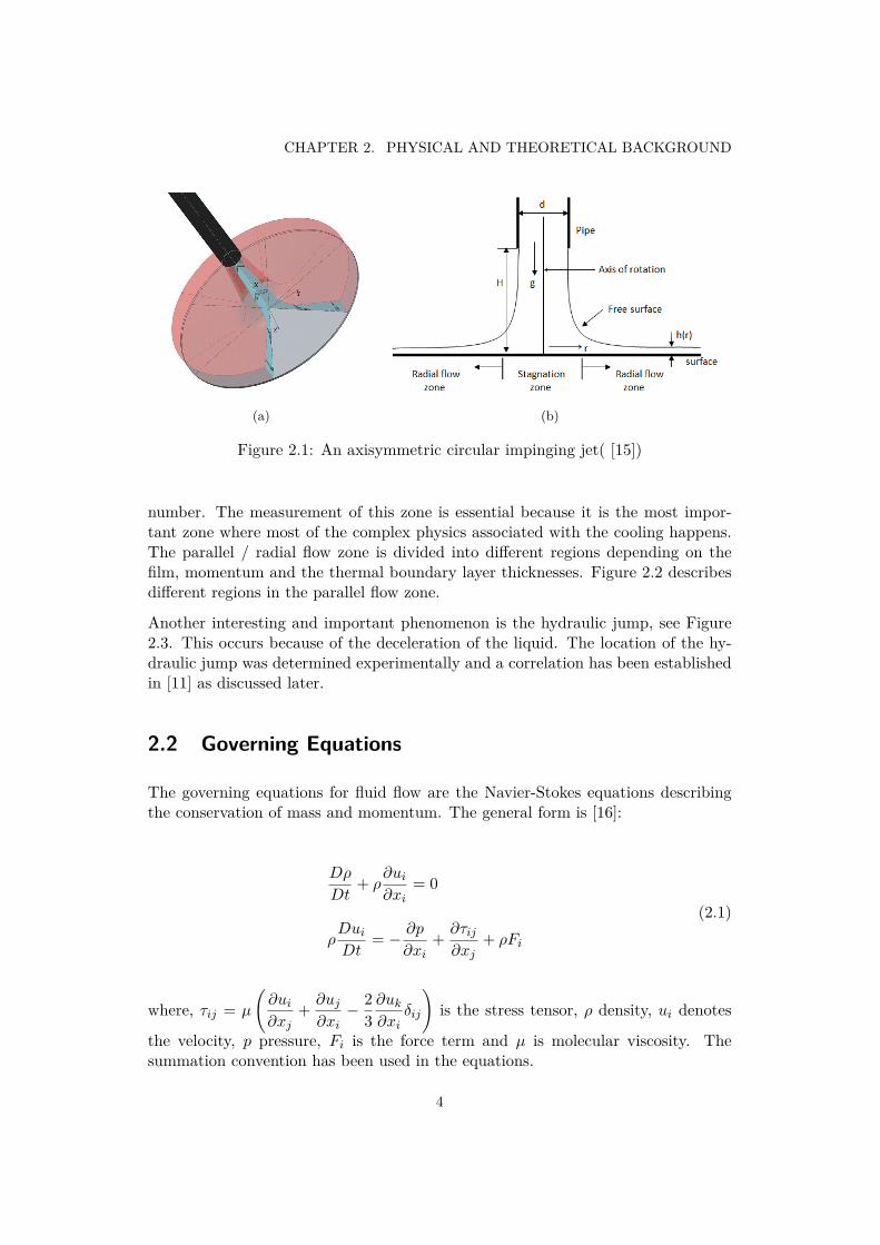
Two types of jets are used for cooling, the free surface liquid jet and the submergedjet. For free surface liquid jets into gas the entrainment of the surrounding fluidis minimal whereas it is significant for the submerged case. The shape of the freesurface is determined by the gravitational force, pressure, and surface tension. Allthese forces are effected by the shape of the jet nozzle and also by the speed of thewater at nozzle exit. In the present study we will consider the free surface liquidjet. Figure 2.1 shows a typical free surface axisymmetric liquid jet configuration.

In figure 2.1 (b), we can see the Stagnation zone beneath the jet nozzle and outsidethis region the Radial or parallel flow zone. The width of the stagnation zone de-pends on the jet diameter, distance between the nozzle and plate and the Reynolds

3

CHAPTER 2. PHYSICAL AND THEORETICAL BACKGROUND

(a) (b)

Figure 2.1: An axisymmetric circular impinging jet( [15])

number. The measurement of this zone is essential because it is the most impor-tant zone where most of the complex physics associated with the cooling happens.The parallel / radial flow zone is divided into different regions depending on thefilm, momentum and the thermal boundary layer thicknesses. Figure 2.2 describesdifferent regions in the parallel flow zone.

Another interesting and important phenomenon is the hydraulic jump, see Figure2.3. This occurs because of the deceleration of the liquid. The location of the hy-draulic jump was determined experimentally and a correlation has been establishedin [11] as discussed later.

2.2 Governing Equations

The governing equations for fluid flow are the Navier-Stokes equations describingthe conservation of mass and momentum. The general form is [16]:

Dρ

Dt+ ρ

∂ui∂xi

= 0

ρDuiDt

= − ∂p

∂xi+ ∂τij∂xj

+ ρFi

(2.1)

where, τij = µ

(∂ui∂xj

+ ∂uj∂xi− 2

3∂uk∂xi

δij

)is the stress tensor, ρ density, ui denotes

the velocity, p pressure, Fi is the force term and µ is molecular viscosity. Thesummation convention has been used in the equations.

4

2.2. GOVERNING EQUATIONS

Figure 2.2: Different zone of an Axisymmetric impinging jet [8], where, Region I: TheStagnation zone, Region II: The laminar boundary layer where the momentum boundarylayer δ is smaller than the liquid film thickness h(r), Region III: The momentum boundarylayer reaches the film surface, Region IV: This is the region from transition to turbulentwhere the momentum and the thermal boundary layer both reach the liquid surface, RegionV: The flow is fully turbulent, Tf is fluid temperature, Uf is fluid velocity at inlet, Um isthe free stream velocity, δ viscous boundary layer thickness, r0 radius at which the viscousboundary layer reaches the free surface, rt the radius at which turbulent transition beginsand rh is radius at which turbulence is fully developed

In Equation (2.1), the derivative term D

Dt= ∂

∂t+uj

∂

∂xjcalled the material deriva-

tive.

In some cases the density change is negligible and considering ρ = constant theequation (2.1) reduces to the incompressible form [16]:

∂ui∂xi

= 0

∂ui∂t

+ uj∂ui∂xj

= −1ρ

∂p

∂xi+ ν∇2ui + Fi

(2.2)

5


Figure 2.3: Visualization of hydraulic jump(picture taken from a sink at home)

Where ν = µ

ρis the kinematic viscosity. In the incompressible form of Navier-Stokes

equations, the conservation of mass equation becomes a divergence free constraintfor the momentum equation and using that constraint the stress tensor term τij in

Equation (2.1) becomes ∂2ui∂xj∂xj

= ∇2ui .

Turbulence model equations

For turbulent flow, most commercial software uses the Reynolds Averaged Navier-Stokes equations (RANS) model. It takes less computational effort than the time-accurate equations and is robust for a wide range of fluid flows. It is derived fromthe standard equations by averaging after decomposing the flow variables into meanand fluctuating components like φ = φ+ φ′ , where φ is the mean (time averaged)and φ′ is the fluctuating component of variables like velocity, pressure or otherscalar quantity. This formulation leads to the continuity and momentum equationsas follows [41]:

∂ρ

∂t+ ∂

∂xi(ρui) = 0

∂

∂t(ρui) + ∂

∂xj(ρuiuj) = − ∂p

∂xi+ ∂

∂xj[µ(∂ui

∂xj+ ∂uj∂xi− 2

3δij∂ul∂xl

)] + ∂

∂xj(−ρu′iu′j)

(2.3)

Note the Reynolds stress term (−ρu′iu′j) which requires additional modeling to close

6

2.2. GOVERNING EQUATIONS

the RANS equations. The Boussinesq hypothesis can be used to relate the Reynoldsstress to the mean velocity gradients as follows:

−ρu′iu′j = µt(∂ui∂xj

+ ∂uj∂xi

)− 23(ρk + µt

∂uk∂xk

)δij (2.4)

Where µt is the turbulent viscosity and k is the turbulent kinetic energy.

This modeling is available with k − ε and k − ω in FLUENT which requires tosolve another two transport equations, for example for turbulent kinetic energy kand ε turbulent dissipation rate in the k − ε model used for all our simulations asturbulence model. There are also several version of the k − ε equations. We usedthe Realizable k − ε model since it predicts the spreading rate for axisymmetric aswell as planar jets very well, according to Fluent theory guide, Ver 14.5 : sec:4.3.3.2.For details of these equations and the modeling we refer to the Fluent Theory Guideand User Manual [41].

Convective Heat and mass transfer

Our study requires to solve the energy equation with the k − ε model. The energyequation is [41]:

∂

∂t(ρE) + ∂

∂xi[ui(ρE + p)] = ∂

∂xj(keff

∂T

∂xj+ ui(τij)eff ) + Sh (2.5)

Where, E is the Total Energy, T is temperature, k is thermal conductivity, keff =

k + CpµtPrt

the effective thermal conductivity, Prt - Turbulent Prandtl number,(τij)eff the deviatoric stress tensor and Sh is source term.

In the convective heat transfer model for the Jet impingement, the analyzed quan-tities are the heat transfer coefficient h and the non dimensional heat transfer co-efficient, the Nusselt number Nu, at the wall surface. The convective heat transfercoefficient is calculated from the heat flux q′′ at the wall surface by,

q′′ = h(Ts − T∞) (2.6)

where, Ts and T∞ are the surface temperature and the free stream fluid temperaturerespectively.

The local surface heat flux can be obtained by using the Fourier law of heat con-duction at the boundary layer by,

7


q′′ = −kf∂T

∂y

∣∣∣∣y=0

(2.7)

The Nusselt number Nud based on diameter of the nozzle can be calculated fromthe heat transfer coefficient h by,

Nud = hd

kf(2.8)

where, d is the diameter of the jet nozzle and kf is the heat conductivity of fluid.

Interface Capturing method

The impingement of water jet is a free surface flow which was modeled by theVolume of Fluid method (VOF). It calculates the volume fraction of liquid in allthe control volumes (or, cells) and depending on the value of the volume fractionit finds the cells that contain the interface. If the volume fraction αq for phase qis 0 then the cell is empty, if 1 then the cell is full but if 0 < αq < 1 then the cellcontains the interface. Then a method called Geometric Reconstruction can be usedto approximate the interface in those cells containing the interface by a piecewiselinear interpolation approach. Another option could be to solve the VOF equationwith the Level-Set method. The VOF-equation that is solved in VOF model is [41]:

1ρq

[ ∂∂t

(αqρq) +∇ · (αqρq−→vq ) = Sαq +∑np=1 (mpq − mqp)] (2.9)

Where,mpq is the mass transfer from phase p to phase q.mqp is the mass transfer from phase q to phase p.Sαq is source term and ρq is the density for phase q.

For further details of the methods used see the FLUENT theory guide [41].

8

Chapter 3

Literature Review

Much theoretical and experimental work has been done on the impinging jet ona flat surface but numerical simulations are rare in this field. In this chapter wediscuss analytical and experimental work by other authors.

Since it is a direct measure of the heat transfer coefficient, the Nusselt numberstudy is very important. The Nusselt number Nu0 at the stagnation point has beendescribed as a function of Reynolds number Re and the Prandtl number Pr bysome authors as

Nu0 = CPrmRen (3.1)

The values of C, m and n were fitted to the analytical solution of the boundarylayer equations or experiments. Many correlations for the Nusselt number outsidethe stagnation zone have been established. Outside the stagnation zone the Nusseltnumber correlations are thoroughly investigated only for laminar flow whereas forturbulent flow different authors summarized different results. It has been observedthat turbulent heat transfer is very different from laminar cases. The experimen-tal results follow the analytical correlations very well for laminar jets but not forturbulent jets.

There are two types of boundary conditions in common use, the constant tempera-ture and the constant heat flux at the wall surface. Boiling is not considered sincewe assume low wall temperature.

Liu and Lienhard in [9] have used an integral method to solve the energy equationanalytically and studied the temperature distribution and the Nusselt number usinga constant heat flux surface. They have compared the experimental data and thetheoretical data for Reynolds number up to 5.27×104 and reported a good agreementwith the theory.

9

CHAPTER 3. LITERATURE REVIEW

Ma et al. in [5] have used an integral method to study the laminar free surfaceaxisymmetric jet considering an arbitrary heat flux condition at the surface. Theyhave established a Nusselt number correlation.

Stevens and Webb in [11] studied the heat transfer coefficient for an axisymmetricliquid jet for a uniform heat flux surface. They have provided a different correlationfor the stagnation point Nusselt number that includes the jet to the plate spacingand also the free stream velocity as in equation 5.2. According to these authors, theconservation of mass near the stagnation zone suggests to scale of the stagnationpoint Nusselt number by using (uf/d) where uf is the free stream velocity. Thiscorrelation gives a slightly higher value according to [1].

Lienhard in [8] has summarized the stagnation zone Nusselt number and has dis-cussed turbulent jets. He mentioned that the Nusselt number at the stagnationzone for uniform wall temperature and uniform heat flux boundary conditions areidentical with no relation to the distance from the impinging point. He reportedgood agreement with the theory and experiment for laminar cases, however it wasemphasized that the turbulent jets can increase the heat transfer coefficient by30− 50%.

Webb and Ma in [10] report a detailed study of the laminar axisymmetric andplaner jet. They have also summarized the correlations for different regions givenby other authors. They observed the experimental data to obey the theoreticalpredictions up to a certain diameter before the transition to the turbulence occursbut it deviates for the turbulent jets. However, the laminar jets behaved accordingto the theoretical prediction. They have summarized that there were some errorsin the stagnation zone prediction. According to them the turbulence yields muchhigher heat transfer and the laminar models then serve as a lower bound for thelocal heat transfer.

Liu et al. in [1] has investigated the single phase laminar liquid jet heat transferof the surface at a constant heat flux. They noted that the Nusselt number showsa peak downstream at the turbulence transition point. The peak corresponds tothe point where the turbulence becomes fully developed. If the Reynolds numberincreases, the peak becomes more pronounced and occurs a short distance from theimpinging point as we found in our study (Illustrated in chapter5). Ma in [4] alsofound this sort of hump from his experiments for different fluids with large Reynoldsand Prandtl number.

The Nusselt number is heavily dependent on the nozzle diameter [11] and thePrandtl number. For high Prandtl number the regions divided into Figure 2.2can be different because the Prandtl number relates the thicknesses of the thermaland viscous boundary layer as δT = δ√

Prwhere δ and δT is the viscous and thermal

boundary layer thickness respectively and Pr is the Prandtl number. The Prandtlnumber of water at 20◦C is 7.0, and in this case the thermal boundary layer is

10

thinner than the viscous boundary layer [1], [8]. It means that, for this case theRegion IV will not occur.

The literature review in this chapter indicates that the heat transfer behavior forturbulent jets is still not very clear. In our simulation cases we have Reynoldsnumber at the jet from 3× 104 to 1.5× 105 which are turbulent. In Chapter 5 thesimulations are compared with the standard correlations from the literature.

11

Chapter 4

Computational domain and Mesh

2D-Axisymmetric Model:

The computational domain geometry and mesh were built using Ansys Workbench14.0. The domain was chosen as small as possible to minimize the number of meshelements. Figure 4.1 shows the geometry and the boundary conditions and Figure4.2 shows the mesh for the 2D axisymmetric case.

Figure 4.1: Geometry of the 2D-Axisymmetric Case

The 2D-axisymmetric mesh is structured with perfect quadrilateral cells. A veryfine mesh was generated around the pipe down to the wall to capture the interfaceand in the boundary layer at the wall surface. The mesh quality is presented intable 4.1.

3D Models:

In the 3D model, symmetry was considered and only half of the domain was modeled.The 3D geometry is shown in Figure 4.3, where the XY-plane is the symmetry planeand the ZX-plane is the wall surface. Except the inlet and pipe (see figure) all theother planes were considered as pressure outlet.

13

CHAPTER 4. COMPUTATIONAL DOMAIN AND MESH

Figure 4.2: Mesh of the 2D-Axisymmetric Case

Figure 4.3: Geometry for the 3D 1-jet model

In the 3D mesh the cells were concentrated around the jet and at the wall surface asit was in 2D. Hexahedral elements were used and a smooth transition between thecell layers was maintained for better accuracy. The mesh only for the 1-jet modelis presented here because the 2-jet mesh does not differ much from the 1-jet mesh.For the 2-jet case we used 2 symmetry planes (XY plane and the left YZ plane)with a fine mesh along the YZ symmetry plane to capture the collision between thetwo jets.

The mesh for the 1-jet model is presented in Figure 4.5 and 4.6. The mesh qualityis presented in table 4.1. The quality of mesh is decided depending on some proper-

14

(a) (b)

Figure 4.4: 3D 2-jet geometry (a) Real computational domain (b) Computationaldomain after applying the symmetry

ties of the cells in FLUENT. In table 4.1 different column shows different propertieswhere the aspect ratio is the ratio of the largest and smallest edge of a cell. Or-thogonal quality and skewness measures cell shape. Y+ value is the dimensionlessdistance from the first cell center to the wall. The mesh quality is good accordingto FLUENT user manual.

Model Total Cell type Max Aspect Min Orthogonal Max Y+ valueelements Ratio quality Skewness at surface

2D- 26890 All Quad 37 1 No 2∼15Axisymmetric skewed cell

3D 1-jet 1,357,632 All Hex 44 0.74 0.55 4∼303D 2-jet 1,621,835 All Hex 51 0.70 0.57 4∼33

Table 4.1: Mesh information for all the models

Figure 4.5: Full mesh for the 3D 1-jet model

15

CHAPTER 4. COMPUTATIONAL DOMAIN AND MESH

(a) (b) (c)

Figure 4.6: 3D 1-jet mesh (a) Zoomed(beam) (b) Zoomed (pipe top) (c) ZoomedSymmetry plane

16

Chapter 5

Results and Discussion

In this chapter the results for the 2D-axisymmetric model, 3D 1-jet model and 3D2-jet model are presented. Results of the 2D-axisymmetric model are comparedwith the analytical solutions from the literature and the results from the 3D modelsare compared with that of the 2D-axisymmetric model.

For the 2D Axisymmetric model we have done 5 simulations with a constant tem-perature and one simulation with constant heat flux boundary condition at the steelsurface. For the single jet 3D model a constant temperature of 100◦C and a constantheat flux boundary condition were considered with a water speed 5 m/s at the inlet.For the double jet model the mesh size was increased significantly and this is whyonly one simulation with constant temperature boundary condition was done forthis case. All the 2D Axisymmetric simulations and the 3D single jet simulationswere done using psudo transient solver in ANSYS FLUENT. On the other hand,the 3D 2-jet case were simulated in a transient solver because the 2-jet simulation isan unsteady process due the collision of the film from two jets. the pseudo-transientsolution method is a form of implicit under-relaxation for steady-state cases. Thismethod uses a pseudo-transient time-stepping approach and it allows us to obtainsolutions faster and more robustly.

The sheet temperature was considered low to avoid boiling. Heat transfer properties:the heat transfer coefficient and the Nusselt number were calculated for differentwater speeds in the range 1 - 5 m/s . The water temperature at inlet was 20◦Cand the plate was kept at constant temperature of 100◦C. Constant heat flux at thestrip surface was also considered for a nozzle speed of 5m/s.

In all the simulations the jet diameter d = 30mm and the distance from nozzle towall surface z = 200mm were held constant. The radial distance of the domainoutlet from the impinging point was chosen as 600mm. So, in our case the resultsare presented up to 20 nozzle diameters from the impinging point.

17

CHAPTER 5. RESULTS AND DISCUSSION

5.1 2D- Axisymmetric model

Figure 5.1: Velocity vector plot of the stagnation zone

The impinging point is directly beneath the jet nozzle center with highest pressureand at the same time the velocity vanishes: a stagnation point. Because of thehigh pressure the water accelerates parallel to the surface. Most of the physicalchanges happen in the stagnation zone. The velocity gradient creates shear stresswhich leads to high heat transfer according to the Reynolds analogy between shearand heat transfer. At the stagnation zone there is a very thin thermal boundarylayer which remains constant [10], but when the water accelerates parallel to thesurface the boundary layer grows and the flow regime transitions from stagnationto boundary layer [1], where the maximum heat transfer occurs. After that theheat transfer coefficient decreases gradually downstream. The characterization ofthe regions in figure 2.2 is basically for a laminar jet and the zonal division can bemuch different for high Reynolds number. The flow behavior at the stagnation zonecan be observed from the velocity vector plot of the stagnation zone in figure 5.1.

Interface

The Volume of Fluid (VOF) method was used to simulate the free surface flow witha high resolution interface capturing method named Geometric Reconstruction forall our simulations. The interfaces between the two phases (air-water) for differentinlet water velocity (u0 = 1ms−1−5ms−1) are shown in figure 5.2. The jet diameterdecreases downwards from acceleration by gravity,

d/d0 = (1 + 2g(z − z0)/u20)−1/2

is clearly seen for lower water speed (See figure 5.3). Here, d0 is the initial diameterand z0 is the distance between the jet and the strip. The narrowing of the jet atimpact influences the position of highest heat transfer coefficient as discussed later.

Film Thickness

The correlation (5.1) was given by Liu et al. in [1] for the liquid film thickness h(r)on the surface starting from the radial position r0 = 0.177dRe1/3

d .

h(r) = 0.1713d2

r+ 5.1417

Red

r2

d(5.1)

18

5.1. 2D- AXISYMMETRIC MODEL

Figure 5.2: Interface shape for different water velocity at inlet

We have compared the correlation in (5.1) with the simulations data in Figure 5.4and found a very good agreement with a maximum 3% deviation. But of course thecorrelation in equation 5.1 does not consider the hydraulic jump. It can be used asa very good estimator for the liquid film thickness from r0 to the position beforethe hydraulic jump.

Nusselt Number

As mentioned before that, many author have established many correlations fordifferent regions showed in figure 2.2 which produce a smooth curve for the Nusseltnumber but for high Reynolds numbers the region division does not follow in thesame way that is why it was very difficult to get a smooth curve by the existingcorrelations. Webb and Ma in [10] have considered the stagnation zone as r <0.4 to 0.8d where d is the diameter of the jet and r is radial distance from theimpinging point whereas Liu et al. in [1] have defined the stagnation zone as r <0.787d.The Nusselt number Nu0 at the stagnation point from our simulations has beencompared with three other existing correlations as a function of Reynolds numberin figure 5.5. Since the thermal boundary layer is constant at the stagnation zone,the Nusselt number results are valid for either uniform wall temperature or theuniform heat flux( [10]). Therefore the comparison at the stagnation zone can bemade regardless of the boundary conditions.

19


(a) (b)

Figure 5.3: Volume Fraction (a) 1ms−1 (b)5ms−1

Steven and Webb(1989) in [11] have given a correlation for the Nusselt number atthe stagnation zone Nu0 from their experiments for a turbulent jet,

Nu0 = 2.67Re0.57d

(z

d

)−1/30 (ufd

)−1/4Pr0.4 (5.2)

where z is the distance from nozzle to the plate, uf is free stream velocity and d isthe diameter of the jet.

According to Joo, P. H. ( [12]), Steven et al.(1992) have given another correlationfor stagnation heat transfer which is:

Nu0 = 0.93Re1/2d Pr0.4 (5.3)

Lui et al. in [1] established the correlation for stagnation zone from their laminaranalysis, as:

Nu0 = 0.787Re1/2d Pr1/3 (5.4)

20


Figure 5.4: Water film thickness comparison

From figure (5.5) it can be seen that the correlation (5.2) gives the highest Nusseltnumber since it considers the free stream velocity of the liquid with the correlation,which is much higher than the Nusselt number from our simulations. On the otherhand, the other two correlations give lower values compared to our results becausethese correlations are for laminar flow and according to [8] the turbulent Nusseltnumber may increase by 30% to 50% from the laminar one. According to all thesecorrelations we have reasonable results.

Liu et al. gave the correlations for different regions of the boundary layer for thelaminar cases with a constant heat flux surface in [1], which are presented in table5.1. They provided correlations to measure the border of different regions too.

Now, in figure 2.2, r0 = 0.1773dRe1/3d is the border of Region II and rt = 1.2× 103d

Re0.422d

is the border of Region III. But if Red > 1.1 × 105 then rt < r0 and the regiondistribution in figure 2.2 becomes invalid ( [1]), as in our case, because we haveReynolds number 1.5×105. Therefore comparisons were made with the correlationsup to Region II. Figure 5.6 compares the Nusselt number from the simulation resultsfor Reynolds number 1.5× 105 with the correlations in table 5.1 up to 5d from theimpinging point. We can see that the patterns of the Nusselt number curves aresimilar and the maximum value occurs almost at the same place but the levels arehigher, as expected, for turbulent flow.

21


Figure 5.5: Comparison of nusselt numbet at the stagnation point with theory

Region Range Nud

Stagnation Zone 0 ≤ r/d < 0.787 , Pr > 3 0.797Re1/2d Pr1/3

Transition: Stag. to b.l. 0.787 < r/d < 2.23

2780RedPr

r

δ12

( rd

)2− 0.2535

1/3

δ = 2.679(rd

Red

)1/2

b.l. Region II 2.23 < r/d < 0.1773Re−0.422d 0.632Re1/2

d Pr1/3( rd

)1/2

Table 5.1: Correlation for Nusselt number for different boundary layer regions by [1]

Figure 5.7 shows the Nusselt number for different flow rates in 2D-axisymmetriccases with a constant temperature boundary condition at the plate. We can seethat all the curves have similar pattern but the maximum value occurs at differentpoints. As the water velocity decreases, the peak gets closer to the axis. This isbecause the water beam diameter decreases for lower speed which has an impact onthe stagnation zone radius. The definition of the stagnation zone is not very clearfrom the literature. All the papers consider the radius of the stagnation zone as aconstant with respect to the jet diameter. They did not consider the flow rate orthe Reynolds number while measuring the stagnation zone except [11]. From our

22


Figure 5.6: Comparison of Nusselt number with theory upto 5 diameter from impingingpoint

simulation results it can be summarized that the radius of the stagnation zone hasconnection with the minimum diameter of the water beam between jet nozzle exitand the surface. The diameter of the water beam is influenced by the velocity atthe nozzle exit and the distance between the nozzle and the plate. If this two areconsidered with the stagnation zone Nusselt number measurement then it is obviousto get very high values as we can see in figure 5.5 and 5.6.

Hydraulic jump

In Figure 5.2 we can see a hydraulic jump at 500mm for 1ms−1 water velocity andReynolds number 3×104. A correlation was given as a function of Reynolds numberby Stevens and Webb in [11]. The position of the hydraulic jump was measured forRe up to 2× 104. The correlation agrees with experiment with an average error of15%.

rhj = 0.0061dRe0.82d (5.5)

Their correlation was derived for a nozzle diameter up to 8.9mm whereas we havethe nozzle diameter 30mm. The nozzle diameter would influence the location of thehydraulic jump. We have 5 different Reynolds numbers and we got hydraulic jumpat 500mm only for the smallest Re 3×104. For higher Re the jump is expected to beoutside the computational domain as the position is proportional to Re accordingto the relation 5.5.

23


Figure 5.7: Nusselt Number for different water speed at inlet

5.2 3D 1-jet model

The 3D models are compared with the 2D-Axisymmetric models, considering the2D cases as reference for the 3D cases. Two simulations were done at a water veloc-ity 5m/s. One is with constant heat flux and the other with constant temperatureboundary condition. In figure 5.8 it can be seen that the 3D models give higherNusselt number at the stagnation point, otherwise the numbers are almost samedownstream. The Nusselt number curves for the 2D and 3D with constant temper-ature boundary condition are the same outside the stagnation zone and the sameholds for the constant heat flux boundary condition, although the constant heatflux boundary condition gives a slightly higher value than the constant temperaturedownstream for both 2D and 3D cases. However, the Nusselt number at the stag-nation zone is found to be the same regardless of the boundary conditions for both2D and 3D cases as Webb and Ma described in [10]. In figure 5.10 we can see thatthe film heights are exactly the same for 2D-Axisymmetric, 3D 1-jet and 3D 2-jetmodel with water velocity 5m/s.

5.3 3D 2-jet model

The 3D 2-jet model seemed to be very difficult to simulate in Fluent. When thefilms from two jets collide, there was too much splashing which leads to convergence

24

5.3. 3D 2-JET MODEL

Figure 5.8: Nusselt number comparison between different boundary conditions

Figure 5.9: Nusselt Number comparison between 2D and 3D models

problem. Because of that problem the jet distance was increased to 400mm toreduce the splashing but it was very difficult to have a steady solution. Therefore,the simulation was re-done in transient mode. Finally the convergence was goodbut simulation is still questionable because of the formed wave due to the collision.The residual for the continuity equation was about 10−2 and the residual for theother equations were below 10−5 but they were fluctuating all the way, this might

25


Figure 5.10: Interface comparison between 2D and 3D models

be because of the wave after collision. In figure 5.9 we can see that the 3D-2 jetmodels agree with the 3D-1 jet model. Figure 5.11 shows the effect at the cornerof the two symmetry plane which tells the flow pattern after collision. Some waterwas flowing outside the domain along the line of collision through the top surfacewhich was a pressure outlet, which results in back flow into the domain and thisis somewhat unphysical for the simulation. Then we increased the domain heightbut still the water was flowing outside. After all, it is obvious to have overall highheat transfer with two jet compared to the 1-jet model because of the position ofthe jets and high water flow rate. In Figure 5.9 the Nusselt number curve ends ata location r/d = 13.33 since the jets are 400 mm apart.

Convergence and Conservation

For all the simulations the conservation of different properties were ensured. Theresidual for the continuity equation was about 10−3 and for rest of the equations itwas below 10−6. For the 2D-Axisymmetric and 3D 1-jet models there was almostno fluctuation. However, there were fluctuations in all the residuals for the 3D 2-jetcase as mentioned before.

26

5.3. 3D 2-JET MODEL

Figure 5.11: Volume of fluid for the 2-jet simulation in 3D shows the splashing at YZsymmetry plane which occurs due to the collision of two waves from two jets

27

Chapter 6

GPGPU

The growth in computational power in the last few years has enabled great stridesin the development of computational sciences, and recently, hardware for graphicshas attracted attention. Graphic cards are generally designed for high resolutiongraphics or for video games, but graphic card manufacturers like Nvidia and AMDhave developed cards that can be used for general purpose computing. This has cre-ated the GPGPU (General Purpose Graphic Processing Unit) parallel programmingparadigm. The latest graphic card has more than 2000 GPU cores and a single pre-cision floating point performance of 3.95 Tflops and double precision floating pointperformance 1.31 Tflops. The card fits into a single workstation, consumes lesspower than a cluster but provides a great speed up compared to a single CPU.Different programming modules also have been developed to use this new platformefficiently. At present there are two , CUDA (Compute Unified Device Architec-ture) and OpenCL (Open Computing Language) which can be used with C, C++,python and many other programming languages. Another package named OpenGLcan be used to visualize simulation outputs with very high resolution. A number ofsimulations have been done in molecular dynamics, fluid dynamics, acoustics andmany other branches using GPGPU.

In this study we have implemented a 2D Navier-Stokes solver in GPGPU in theC programming language. In this paper different methods that are implementedby other people on GPGPU have been discussed. Moreover, the achieved speedup,the performance of our solver along with the discussion of various optimizationtechniques and the difficulties in coding are presented. We have chosen the OpenCLpackage because it is an open standard supported by several manufacturers whereasCUDA is supported only by NVIDIA.

29

CHAPTER 6. GPGPU

6.1 Different Methods

This study focuses on methods for Computational Fluid Dynamics. The governingequations for any simulation is the Navier-Stokes equation. There are simplifiedmethods based on grids or particle or hybrid. Methods based on grids are calledthe Eulerian methods and the methods based on particle are called Lagrangianmethods. Both methods have their own advantages and disadvantages but someavailable hybrid methods combine both to get the benefit from both type of methods.

Grid or Mesh based methods

Methods like Finite Difference, Finite Volume, Finite Element etc. are developedbased on grids. In CFD the most widely used method is the Finite Volume method(FVM). It is a purely mesh dependent method and while solving Navier-Stokesequation one solves the continuity, momentum or vorticity and energy equation (ifrequired) in a checker board (staggered grid) fashion. For time dependent flows thecommon way to solve the discrete equations is the so-called projection or pressurecorrection method (Sometimes called splitting methods). For detailed derivationand discretization of FVM and Projection method we refer to [16]. In our OpenCLimplementation this method was chosen to solve the time dependent incompressibleNavier-Stokes equation (2.2) and Conjugate Gradient (CG) Method was imple-mented to solve the algebraic system in the pressure correction part. For the detailsof the CG method we refer to [17].

Simplified models like Jos Stam’s "Stable fluids" in [27] have been developed forfaster fluid simulations. This is a very popular method for fluid simulation in Com-puter graphics and animation. Another popular method for fluid flow in computergraphics is the so called staggered Marker and Cell (MAC) grid for free surfaceflows. Nowadays, also the level set method is widely used for interface tracking. Atwo phase flow has been simulated using level set method on GPU in [35].

A different class of method for fluid simulation is the Lattice Boltzmann method.These methods execute cellular automata which emulate the Boltzmann equationand can be averaged to produce solutions to the Navier Stokes equation. Severalimplementations of these methods have been done using GPGPU, for example in[32].

Particle based methods

Fluid particle simulation comes in two major varieties: Smoothed Particle Hydro-dynamics (SPH) and Discrete Vortex Methods (DVM). SPH uses fluid particlesto represent flow whereas DVM uses vortex particles called "vortons" which rep-resent tiny vortex elements. These methods are usually implemented using a treestructure and the Fast Multipole Method (FMM) to calculate interaction betweenparticles, which is a very well known method for particle simulation. [33], [34] have

30

6.2. WHY OPENCL?

used SPH, [29], [30] used FMM and [36], [38], [39] used vortex particle method tosolve different problems on GPU.

Hybrid methods

This methods uses the backtracking style called Semi-Lagrangian technique. Ittransfers the vortex particle into a grid and then solves the Poisson equation on thegrid to get the velocity field. These methods are known as Particle in Cell (PIC) orVortex in Cell (VIC). Details of implementation techniques for these methods aredescribed in [40]. Some details of hybrid methods, Multiresolution method, adap-tive meshing techniques, interface capturing particle methods and about differentboundary conditions have been discussed in [19].

6.2 Why OpenCL?

CUDA and OpenCL both have their own advantages. CUDA is a bit older thanOpenCL which has more libraries and a bit easier to use for the programmers, butit is only supported by Nvidia cards. On the other hand, OpenCL is a platformindependent module. It is a programming package which can run on heterogeneoussystems that use GPGPUs, GPUs, CPUs, or any other parallel programming device.Once you write your code, you can run it on any parallel device which is really great,this is why we have chosen OpenCL for our implementation. In contrast, writingan optimized code using OpenCL is much more difficult than CUDA. One has tothink about the portability which requires extra care while designing the algorithmand may have performance penalties. It is very hard to write a code which can runon different platforms with the same performance. It might be wise to leave thetask to the platform it works better and also switching between platforms to getthe best out of the available resources.

6.2.1 OpenCL basics

In order to understand the OpenCL, one needs to know some OpenCL terms, pro-gramming modules and the memory model. There are two parts of an OpenCLprogram: Programming for the Host and Programming for the device (GPUs). Thefirst part is writing the host program like a normal C/C++ program that runs onCPU and the other part is writing the kernels that use some special syntax otherthan normal C/C++ that run on GPUs. The host sets up the environment neededto run kernels on GPUs, create and compile the kernels, transfer the required datafrom CPU memory to GPU memory back and forth, creates and maintains a com-mand queue to initiate any task to the GPU devices, issues command to GPUdevices and finally collects all the results when done.

31

CHAPTER 6. GPGPU

Figure 6.1: A typical GPU platform architecture

Figure 6.1 describes a typical GPU platform architecture where a workstation/clustercontains one or more CPU that works as Host and one or more GPUs that works asthe parallel device. Each GPU device has many compute units (Streaming multi-processors for Nvidia) and each multiprocessor has many processing elements (PE).Processing element corresponds to Scaler processor(SP) for Nvidia.

Workitems :The basic unit of work in an OpenCL device.

Workgroups : Workitems are further organized in to different workgroups. Thereare two different work groups that need to be defined when running an OpenCLkernel: A Local and a Global work group. Global work group size must be divisibleby the Local work group size in each dimension.

Local workgroup : A Local work group is a group of the workitems that willbe executed by a single multiprocessor(Or, Compute unit (OpenCL name)).

Global workgroup : A Global work group is executed concurrently by theavailable multiprocessors in the device. The local and Global workgroup defines theIndex space.

Index Space

Index space is a grid of workitems where each of the workitems has a local id anda global id. Any kernel runs according to the workitems ids. Figure 6.2 describesa N-Dimensional Range index space where Lx, Ly are the local ids within a localworkgroup in x and y dimension. Gx, Gy are global ids and Wx and Wy are localworkgroup ids in x and y direction.

32

6.2. WHY OPENCL?

Figure 6.2: Index space for NDRange [20]

OpenCL Memory Model

OpenCL memory model is the most crucial part in OpenCL programming. Figure6.3 shows the OpenCL memory model together with the interaction between thememory model and the platform model.

Host memory: This is the CPU memory and only visible by the Host.

Global memory: The largest memory in device where all the workitems in allworkgroups and the host have read/write permission.

Constant memory: This a part of global memory that is allocated and initializedby the host which remains constant throughout the kernel execution. Workitemshave read-only permit to this memory.

Local memory: Memory of a multiprocessor which is shared among all theworkitems in a local workgroup.

Private memory: This is a private memory to a single workitem.

For more details of OpenCL programming see [18], [20] and [21].

33

CHAPTER 6. GPGPU

Figure 6.3: OpenCL memory hierarchies [20]

6.3 Algorithm and Implementation

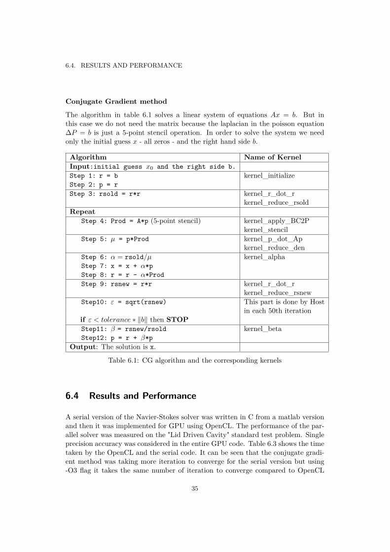
The incompressible Navier-Stokes equation (2.2) and the Energy equation werediscretized using the splitting method described in [16]. This is a straight forwardimplementation of the staggered grid projection method and not discussed here. Theperformance of the solver depends totally on the pressure correction part where onehas to solve the Poisson equation in each time step (see Figure 6.6). The ConjugateGradient method was implemented to solve the system of equations. The ConjugateGradient method algorithm is presented in a table style to link the kernel name withthe algorithm in table 6.1.

In the implementation of CG kernels the main bottleneck was the global reductionin the scalar product and CG is heavily dependent on scalar products. The localmemory was used to aid the global reduction in a efficient way (For details see [24]).Note: There is no global synchronization and no barrier synchronization within theworkitems in different workgroups, which forced us to write many kernels to ensureglobal synchronization and correct data access in different steps of the algorithm.The convergence criterion for CG was checked by the host only in each 50th it-eration because global synchronizations are so expensive. Algorithms with fewersynchronizations and barriers perform better; The Jacobi iteration with multi-gridacceleration should be investigated as an alternative to CG.

34

6.4. RESULTS AND PERFORMANCE

Conjugate Gradient method

The algorithm in table 6.1 solves a linear system of equations Ax = b. But inthis case we do not need the matrix because the laplacian in the poisson equation∆P = b is just a 5-point stencil operation. In order to solve the system we needonly the initial guess x - all zeros - and the right hand side b.

Algorithm Name of KernelInput:initial guess x0 and the right side b.Step 1: r = b kernel_initializeStep 2: p = rStep 3: rsold = r*r kernel_r_dot_r

kernel_reduce_rsoldRepeat

Step 4: Prod = A*p (5-point stencil) kernel_apply_BC2Pkernel_stencil

Step 5: µ = p*Prod kernel_p_dot_Apkernel_reduce_den

Step 6: α = rsold/µ kernel_alphaStep 7: x = x + α*pStep 8: r = r - α*ProdStep 9: rsnew = r*r kernel_r_dot_r

kernel_reduce_rsnewStep10: ε = sqrt(rsnew) This part is done by Host

in each 50th iterationif ε < tolerance ∗ ‖b‖ then STOPStep11: β = rsnew/rsold kernel_betaStep12: p = r + β*p

Output: The solution is x.

Table 6.1: CG algorithm and the corresponding kernels

6.4 Results and Performance

A serial version of the Navier-Stokes solver was written in C from a matlab versionand then it was implemented for GPU using OpenCL. The performance of the par-allel solver was measured on the "Lid Driven Cavity" standard test problem. Singleprecision accuracy was considered in the entire GPU code. Table 6.3 shows the timetaken by the OpenCL and the serial code. It can be seen that the conjugate gradi-ent method was taking more iteration to converge for the serial version but using-O3 flag it takes the same number of iteration to converge compared to OpenCL

35

CHAPTER 6. GPGPU

code. There are two things to note here. GPU has only 32-bit registers whereasa 64-bit computer has 64-bit registers and 80 bits in the implementation of IEEEfloating point arithmetic. Moreover, from the basic of error analysis one can seethat the parallel environment and serial environment should give slightly differentresults specially when working with scaler product of two vectors. In our case theCG method is heavily dependent on the scaler products. On the other hand, -O3flag does some loop reordering and loop unrolling which might have similar issueslike parallel environment, this is why it takes same number of iterations as GPUcode. But, if we think about the convergence then the number of iterations canbe considered as an internal matter and the comparison between the GPU and theserial code is fair.

Workstation Configuration GPU ConfigurationIntel(R) Xeon(R) W3503 Nvidia Tesla C2075Clock Speed: 2.4GHz Computer Unit: 14

Memory : 9GB Memory: 6GBCPU cores: 2 GPU cores: 448

Table 6.2: Computer configuration

Dimension GPU CPUNx=Ny Time(sec) CG iter. Time(using -O3) CG iter.

(Sec)32X32 0.24 201 0.02 20164X64 0.40 351 0.12 351128X128 0.72 651 0.98 651256X256 1.38 1251 7.62 1251512X512 6.45 2451 60.31 24511024X1024 41.60 4851 543.60 48512048X2048 308.70 9651 4300.69 9651

Table 6.3: Time taken by the GPU and Serial code for different problem size for 10time steps

Figure 6.4 shows sample output from the GPU solver visualized using Matlab.The initial condition for the velocity was 1m/s at the lid on the top and a lineartemperature profile was chosen as an initial condition for the temperature. Sincethe flow is laminar (Re = 100) the solution becomes steady after about 10sec.

6.4.1 Speedup

The speedup of the parallel solver was measured comparing with the unoptimizedversion of the serial solver and also with the optimized version using -O3 flag.Due to time constraint, the parallel solver was not optimized but the optimizationtechniques have been discussed in Section 6.4.3. The performance of the solver can

36


(a) (b) (c)

Figure 6.4: Output from the GPU program (a) Problem domain(Filled with water)(b) Contour of Velocity profile (c) Contour of Temperature profile at t=20s withRe=100

be optimized as discussed later. One can have an idea about the speedup using aGPU device compared to a serial code on the CPU from Figure 6.5.

Figure 6.5: Speedup for different problem size

6.4.2 Profiling and Debugging

There are a few debugging and profiling tools for OpenCL program available now.The debugger gDebugger was used to debug the code and the Nvidia ComputeVisual Profiler was used to profile our code. The debugger and the profiler wasused both in windows and linux platform (Ubuntu 12.04). Some useful profilingoutput will be presented in section 6.4.3.

37

CHAPTER 6. GPGPU

6.4.3 Optimization techniques

Before starting the optimization process one needs to profile the code and find thebottleneck of the program. The profiler will give detailed analysis of every kernelthat is running on the GPU device.

Kernel optimization

In the Navier-Stokes solver we have 11 kernels for the Conjugate Gradient methodand 10 kernels for the main solver. Figure 6.6 shows the time taken by each kernelin one time step. From Figure 6.6 we can see that most of the time was taken bythe kernels of the pressure correction part, so the CG kernels are the first targetsfor optimization.

Figure 6.6: Time taken by each kernel in one time step

Now, the question is, how much computational capacity of the GPU device have weused? From the GPU time summary plot in Figure 6.7 one can see that we haveused only about 14% of the total time and about 86% of the time the GPU devicewas idle. It tells us how much room do we have for optimization. Next questionis, why the GPU is idle? In Figure 6.8 different colors are showing the runningtime of different kernels and the white spaces are the idle time between each of thekernel run instances. So the number of kernel should be minimized to reduce theidle time. One can try to launch the next kernel before the previous has finished, tooverlap the idle time by computation. But that is possible only if there is no datadependency of the previous kernel. The kernels in CG have data dependencies. It

38


is wise to choose algorithms or methods that are simple and can be written in away so that they have little data dependency. On the other hand, writing a verybig kernel is not recommended because big kernels will require many registers perworkitem but a single multiprocessor has only few registers.

Figure 6.7: GPU time summary plot which shows the total running and idle time

NDRange optimization

The Global Workgroup size and the Local Workgroup size both have a serious im-pact on the performance of the program. The better choice of the above parametersare chosen, the better the performance is. There is no universal formula for the op-timal size of the Global and Local workgroup. The only way is to experiment withdifferent numbers keeping in mind that the global workgroup size must be divisibleby the local workgroup size in each dimension. Before choosing the numbers youhave to know the hardware very well that you are going to use.

Local workgroup size has certain relation to the alignment of the memory in thedevice and the amount of register that is available in a single multiprocessor. OneLocal work group will run on one multiprocessor and one multiprocessor has alimited amount of register which is divided among all the work items in a localworkgroup. If the requirement of the register exceed the available register, then it

39

CHAPTER 6. GPGPU

Figure 6.8: Idle time of GPU device (snap of one iteration of CG algorithm)

fails to launch the kernel.

Nvidia says that, the local workgroup size should be chosen as a multiple of 32workitems in order to achieve optimal computing efficiency and facilitate coalesc-ing(access consecutive memory addresses). [22]

From Figure 6.9 and 6.10 one can understand the impact of the Local workgroupsize on the performance. In this example the Global workgroup size was keptconstant ( 128X64 ) and the Local workgroup size was chosen 16X8 and 32X4. Thelater one takes total 12.31% less time than the former one. Which is because thelater one is a multiple of 32 and it helps to access the memory in a coalesced(that is,access the consecutive memory addresses) way which gives high memory throughput.

On the other example the Local workgroup size was kept constant 32X4 (Sinceit worked better in previous example) and the Global workgroup size was taken128X64 and 64X64. From Figure 6.11 and 6.12 we can see that the case 64X64took about 40% more time than the case 128X64. Which is because, the actualproblem size is much bigger than the maximum global workitems (Total workitemsin a Global workgroup) and to cover the whole problem one has to iterate on thedata. There are certain limitations on the global workgroup size. We can notjust take the global workgroup as big as we wish. Now, for example we want tosolve the Navier-Stokes equation on a 512X512 grid. The GPU card(Nvidia TeslaC2075) we used for our purpose supports 216−1 maximum workitems which is muchsmaller than 512X512. Only possible way to solve this problem is to loop over thedata. If we iterate on 512X512 grid with a 64X64 global workgroup size than wehave to iterate more compared to 128X64 global workgroup size, this is why globalworkgroup size 64X64 takes more time.

In order to get the best performance from the available hardware one has to tune

40


and experiment with different Global and Local workgroup size and try to find theoptimized value for the used hardware. There is a calculator from Nvidia namedoccupancy calculator which can be used to estimate a suitable workgroup size.

Figure 6.9: Time taken by each kernel in one time step for different local workgroup size

Figure 6.10: Total GPU time taken by the kernels in one time step for different Localworkgroup size

Memory level optimization

One needs to write the kernels in a way so that the Global memory access patternis coalesced to gain high memory throughput. The width of the thread (workitems)block and the width of the accessed array must be a multiple of 32 to access thememory in fully coalesced way [23]. Another way of optimizing a kernel is to uselow latency and high bandwidth memory whenever possible. This is done by usingthe local memory which is shared among all the workitems in a local workgroup.This is 100 times faster than the global memory access but only if there is no bankconflict. Bank conflict happens when two or more workitems try to access the

41

CHAPTER 6. GPGPU

Figure 6.11: Time taken by each kernel in one time step for different Global workgroupsize

Figure 6.12: Total GPU time taken by the kernels in one time step for different Globalworkgroup size

same memory address at the same time. For details of Bank conflict see [20], [23].In our implementation, local memory was used for all the global reductions in thescalar products. The kernel for the matrix-vector product (which is a 5-point stenciloperation) can also be written using local memory.

Instruction optimization

To optimize the code at a instruction level, one should minimize the branching asmuch as possible. Using the single precision instead of double precision is recom-mended if single precision is enough for the purpose. Instruction can be reducedsignificantly by using the native functions like divide, sine, cosine, bitwise operatorinstead of %(The modulo operator) etc. cl_nv_pragma_unroll extension can alsobe used to unroll any loop to avoid branching within a warp (32 workitems). Try

42


to use shared memory instead of global memory to reduce memory instructions.

For more optimization techniques see Nvidia OpenCL Best Practice Guide [22] andOpenCL Programming Guide for the Cuda Architecture [23].

43

Chapter 7

Conclusion and Future Work

Comparing the theoretical and simulation results it can be concluded that Heattransfer CFD simulation is very difficult because of the uncertainty in heat fluxprediction. It is very hard to estimate the heat transfer coefficient using RANSmodel, specially when the flow is turbulent. One can try DNS (Direct NumericalSimulation) simulation for better approximation but it is almost impossible to con-duct DNS simulation for industrial research. GPU usage can be a good solutionin terms of computational power. But it is very hard to write an efficient solverusing GPU platform because one has to take care of every hardware details. Thereare other drawbacks for this platform also, for example the performance is poor forcomplex algorithms. From our case of CG algorithm it can be seen that the globalreduction and applying boundary conditions have great impact on performance. So,it is wise to choose simple algorithm that requires less synchronization to get betterperformance and speedup.

In this present study we have studied the heat transfer phenomenon of a single phaseimpinging water jet with a stationary surface. As we mentioned before that, becauseof very high temperature the boiling phenomenon occurs in the Runout table andthe steel surface has a certain speed. So the next task would be to analyze theheat transfer for a moving surface and also introduce high temperature to studythe boiling phenomenon. The 2D-Navier Stokes solver written in GPU here can beextended to 3D. Other possible way could be to implement the particle or hybridmethods described in section 6.1 in GPU which may reduce the computational effortsignificantly.

45

Bibliography

[1] Liu, X., Lienhard V, J. H., Lombara J. S., 1991, Convective Heat Transfer byImpingment of Circular Liquid Jets. Journal of Heat Transfer, Vol. 113/571

[2] Gardin, P., Pericleous, K., 1997, Heat Transfer by Impinging Jet On a MovingStrip Inter. Conf. on CFD in Mineral & Metal Processing and Power Genera-tion.

[3] Cho, M. J., Thomas, B. G., 2009, 3D Numerical Study of Impinging WaterJets in Runout Table Cooling Processes. AISTech 2009 Steelmaking ConferenceProc., (St. Louis, MO, May 4-7, 2009), Assoc. Iron Steel Tech., Warrendale,PA, Vol.1

[4] Ma, C. F., 2002, Impingement Heat Transfer with Meso-scale Fluid Jets. in:Proceedings of 12 th International Heat Transfer Conference.

[5] Ma, C.F., Zhao, Y. H., Masuoka, T., Gomi, T., 1996, Analytical Study on Im-pingement Heat Transfer with Single-Phase Free-Surface Circular Liquid Jets.Journal of Thermal Science, Vol.5, No.4

[6] San, J. Y., Lai, M. D., 2001, Optimum jet to jet spacing of heat transfer forstaggered arrays of impinging air jets. Int. Journal of Heat and Mass Transfer44 (2001) 3997-4007

[7] Frost, S. A., Jambunathan, K., Whitney, C. F., Ball, S. J., 1996, Heat Transferfrom a flat plate to a tubulent axisymmetric impinging jet. Proc Instn MechEngrs, Vol 211 Part C

[8] Lienhard V, J. H., 2006, Heat Transfer by Impingement of Circular Free-SurfaceLiquid Jets. 18th National & 7th ISHMT-ASME Heat and Mass Transfer Con-ference, January 4-6, 2006

[9] Liu, X., Lienhard V, J. H., 1989, Liquid Jet Impingement Heat Transfer on AUniform Flux Surface. ASME, HTD-Vol. 106, Heat Transfer Phenomenon inRadiation, Combustion, and Fires.

47

BIBLIOGRAPHY

[10] Webb, B. W., MA, C. F., 1995, Single Phase Liquid Jet Impingement HeatTransfer. Advances in Heat Transfer, Vol. 26

[11] Steven, J., Webb, B.W., 1989, Local Heat transfer Coefficients Under an Ax-isymmetric, Single-Phase Liquid Jet. Heat Transfer in Electronics -1989, ASMEHTD-Vol. 111, pp. 113-119

[12] Joo, P. H., Majumdar, A. S., Heat Transfer Under Laminar Impinging Jets:An Overview. Transport Process Research Group, ME, National University ofSingapore.

[13] Incropera, F. P., DeWitt, D. P., Bergman, T. L., Lavine, A. S., 2006, Fun-damentals of Heat and Mass Transfer. Sixth Edition, John Wiley and Sons.Inc.

[14] Mukhopadhyay, A., Sikdar, S., 2005, Implementation of an on-line run-outtable model in a hot strip mill. Journal of Materials Processing Technology,Volume 169, Issue 2, Pages 164-172.

[15] Hallqvist, T., 2006, Large Eddy Simulation of Impinging Jet with Heat Transfer.Technical report, KTH Mechanics.

[16] Henningson, D., Berggren, M., 2005, Fluid Dynamics: Theory and Computa-tion. KTH-Mechanics.

[17] Trefethen, L.N., Bau, D., Numerical Linear Algebra,. ISBN: 0-89871-361-7.

[18] Khronos OpenCLWorking Group, The OpenCL Specification. Version 1.1, Doc-ument Revision:44, Editor: Aftab Munshi

[19] Koumoutsakos, P., Cottet, G-H., Rossinelli, D., Flow Simulations Using Par-ticles. Bridging Computer Graphics and CFD.

[20] Munshi, A., Gaster, B.R., Mattson, T.G., Fung, J., Ginsburg, D., OpenCLProgramming Guide. Addision-Wesley (2012)

[21] Gaster, B. R., Howes, L., Kaeli, D., Mistry, P., Schaa, D., Heterogeneous Com-puting withOpenCL. MK publications.

[22] Nvidia, OpenCL Best Practice Guide. Optimization (2010)

[23] Nvidia, OpenCL programming Guide for the CUDA Architecture. Version 3.2(2010)

[24] Nvidia, OpenCL programming for the CUDA Architecture. Version 3.2 (2010)

48

[25] AMD Accelerated Parallel Processing, OpenCL. May (2012)

[26] Bridson, R., 2008, Fluid Simulation for Computer Graphics,. A K Peters, Ltd.

[27] Stam, J., 1999, Stable Fluids,. Computer Graphics SIGGRAPH 99 Proceedings(1999) 121-128.

[28] Kosior, A., Kudela, H., 2011, Parallel computations on GPU in 3D using thevortex particle method. Computer & Fluids, Elsevier.

[29] Drave, E., Cecka, C., Takahasi, T., 2011, The fast multipole method on parallelclusters, multicore processors, and graphic processing units. Elsevier MassonSAS.

[30] Yokota, R., Narumu, T., Sakamaki, R., Kameoka, S., Obi, S., Yasuoka, K.,2009, Fast Multipole Method on a cluster of GPUs for the meshless simulationof turbulence. Computer Physics Communication, Elsevier B.V.

[31] Xu, S., Mei, X., Dong, W., Zhang, Z., Zhang, X., 2012, Real time ink simulationusing a grid-particle method. Compter & Graphics, Elsevier.

[32] Xian, W., Takayuki, A., 2011, Multi-GPU performance of incompressible flowcomputation by lattice Boltzmann method on GPU cluster. Parallel Computing,Elsevier B.V.

[33] Dominguez, J.M., Crespo, A.J.C., Gesteira, M.G., 2011, Optimization strate-gies for CPU and GPU implementations of a smoothed particle hydrodynamicsmethod. Computer Physics Communications, Elsevier B.V.

[34] Wang, B.L., Liu, H., 2010, Application of SPH method on free surface flows onGPU. Journal of Hydrodynamics.

[35] Kuo, S.H., Chiu, P.H., Lin, R.K., Lin, Y.T., 2010, GPU implementation forsolving incompressible two-phase flows. International Journal of Informationand Mathematical Sciences 6:4 2010.

[36] Rossinelli, D., Bergdorf, M., Cottet, G.H., Koumoutsakos, P., 2010, GPU ac-celerated simulations of bluff body flows using vortex particle methods. Journalof Computational Physics 229(2010) 3316-3333

[37] Junior, J.R.S., Joselli, M., Zamith, M., Lage, M., Clua, E., 2012, An Architec-ture for real time fluid simulation using multiple GPUs. SBC- Proceedings ofSBGames 2012.

[38] Rossinelli, D., Koumoutsakos, P., 2008, Vortex Methods for incompressible flowsimulations on the GPU. Visual Comput (2008) 24:699-708

49

BIBLIOGRAPHY

[39] Selle, A., Rasmussen, N., Fedkiw, R., A Vortex Particle Method for Smoke,Water and Explosions.

[40] Gourlay, M. J.,2012, Fluid Simulation for Video Games (Part 1 - part 15).

[41] FLUENT theory guide and user manual, ANSYS FLUENT 14.5.

50

TRITA-MAT-E 2013:30 ISRN-KTH/MAT/E—13/30-SE

www.kth.se

cfd simulation of jet cooling and implementation of flow

Documents