cfd modelling of isothermal multiple jets … international conference on cfd in the minerals and...

Eleventh International Conference on CFD in the Minerals and Process Industries

CSIRO, Melbourne, Australia

7-9 December 2015

Copyright © 2015 CSIRO Australia 1

CFD MODELLING OF ISOTHERMAL MULTIPLE JETS IN A COMBUSTOR

Shen LONG1*, Zhao Feng TIAN, Graham NATHAN, Alfonso CHINNICI, Bassam DALLY

1 School of Mechanical Engineering, The University of Adelaide, South Australia 5005, Australia *Corresponding author, E-mail address: [email protected]

ABSTRACT

This paper assesses the performance of three turbulence

models on the simulation of an isothermal flow from a

burner with three separated-jet inlets. This burner has key

flow features of a novel hybrid solar receiver combustor

(HSRC) that is under development in the Centre for

Energy Technology (CET) at the University of Adelaide.

Three turbulence models, namely, the Baseline Reynolds

Stress (BSL RSM), the Shear-Stress-Transport (SST) and

the Standard k-ɛ (SKE) models were chosen. The paper

reports numerical results from two cases of the separated-

jet flows. In these two cases, the angle between the side jet

and the centre jet is 0° and 20° . The predicted mean

velocity profiles at six positions of this burner are

compared against experimental results from the literature.

It is found that the best prediction is provided by the BSL

RSM model, which predicts well the velocity peaks and

reproduces the trend of velocity profiles in different axial

positions. Importantly, the BSL RSM model has the

advantage of predicting anisotropic Reynolds stresses in

interacting jet flows. This opens the way to use these

models to inform the development of the combustion

system within the HSRC.

INTRODUCTION

The concept of integrating Concentrating Solar Thermal

(CST) technology and traditional combustion energy is

gaining prominence globally due to the complementary

nature of these two thermal energy sources (Ordorica-

Garcia, Delgado & Garcia 2011). CST can reduce the

emission of greenhouse gas and provide a cost-effective

way to incorporate solar with thermal energy storage

(Steinmann 2012) to overcome the challenge of the

intermittent nature of solar radiation (Jin & Hong 2012).

The integration of combustion energy source with CST

offers a relatively low cost solution which minimises the

need for costly long term energy storage and provides

certainty for baseload power.

A Hybrid Solar Receiver Combustor (HSRC) has been

proposed by the Centre for Energy Technology (CET) at

the University of Adelaide, which is a combination of a

solar cavity receiver and a gaseous fuel combustor. The

HSRC reduces heat losses relative to equivalent hybrids

by integrating CST and combustion energy source into a

single device (Nathan et al. 2013; Nathan et al. 2009). The

HSRC is designed to operate in any of three modes: the

‘combustion only mode’, the ‘solar only mode’ and the

‘mixed mode’. For the ‘solar only mode’, the shutter of

Compound Parabolic Concentrator (CPC) is open to allow

the entry of concentrated solar radiation into the receiver,

so that the heat source for the HSRC is only solar energy.

In contrast, the heat source in the ‘combustion only mode’

is derived only from the burning of injected fuel. In the

‘mixed mode’, the heat source for the HSRC is derived

from both solar radiation and combustion, with the

percentage of each being dependent on the solar intensity

available at the time. A schematic diagram of the HSRC is

presented in Figure 1.

The HSRC is still in the early stages of development.

Owing to the range of operational modes, it can be

expected that different flow regimes, flame structures and

dominant heat transfer mechanisms will occur at different

times inside the HSRC. Hence there is a need to

understand the flow dynamics of this unique geometry to

design burners that can work effectively. Based on the

proposed configurations of the HSRC, multiple burners

are distributed within the conical configuration of the

chamber with an angle of inclination (𝛽𝑗𝑒𝑡) that causes the

jets to interact within the chamber (Figure 1). According

to Chinnici (2015), by changing the inclination angle of

the jet from 30° to 90°, the flow features and combustion

behaviours inside the HSRC change dramatically.

Therefore, a comprehensive understanding of the

influence of interacting jets on flow dynamics inside the

HSRC is desirable.

Figure 1: Schematic diagram of the Hybrid Solar

Receiver Combustor (Nathan et al. 2013).

Prior to building experimental facilities with which to

directly assess the performance of the HSRC, CFD models

have been developed using other experimental data from

related configurations. Of these, the investigation of

interacting jets of an oxy-fuel combustion separated-jet

burner developed by Boushaki and Sautet (2010) was

chosen for CFD model validation. This burner consists of

a central jet of natural gas placed between two oxygen

jets, the orientation of which is adjustable (Boushaki et al.

2008; Boushaki et al. 2007). Hence this system has similar

features to the multiple-jet configuration of the HSRC. A

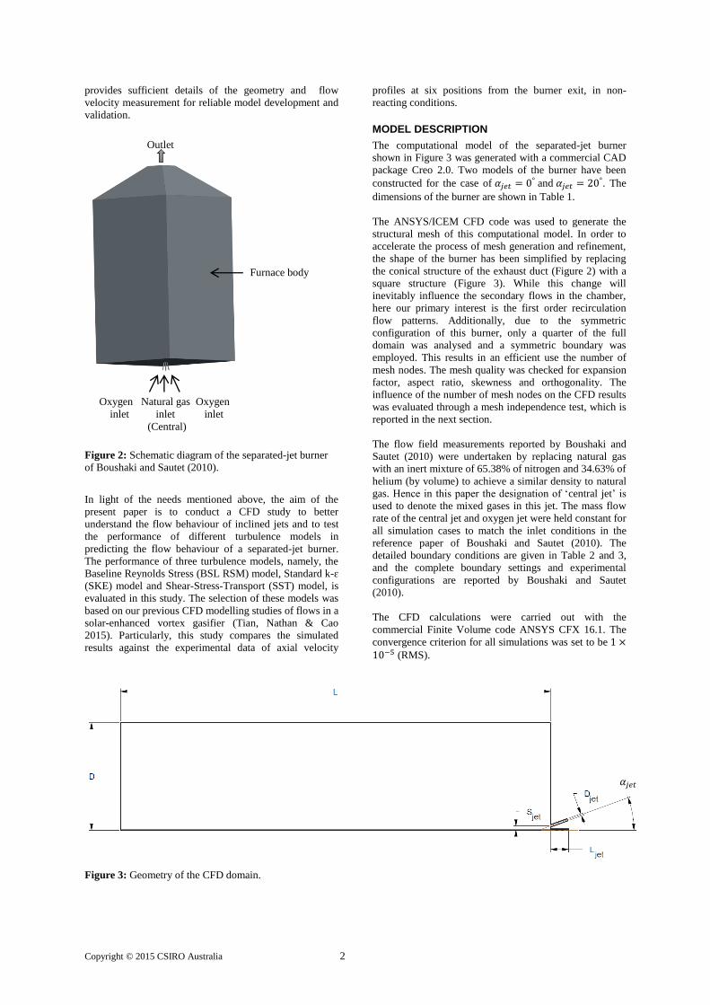
schematic diagram of this system is shown in Figure 2.

Importantly, the work of Boushaki and Sautet (2010)

Concentrated

Solar

Radiation

Jet inlet

Jet inlet

𝛽𝑗𝑒𝑡


provides sufficient details of the geometry and flow

velocity measurement for reliable model development and

validation.

Figure 2: Schematic diagram of the separated-jet burner

of Boushaki and Sautet (2010).

In light of the needs mentioned above, the aim of the

present paper is to conduct a CFD study to better

understand the flow behaviour of inclined jets and to test

the performance of different turbulence models in

predicting the flow behaviour of a separated-jet burner.

The performance of three turbulence models, namely, the

Baseline Reynolds Stress (BSL RSM) model, Standard k-ɛ

(SKE) model and Shear-Stress-Transport (SST) model, is

evaluated in this study. The selection of these models was

based on our previous CFD modelling studies of flows in a

solar-enhanced vortex gasifier (Tian, Nathan & Cao

2015). Particularly, this study compares the simulated

results against the experimental data of axial velocity

profiles at six positions from the burner exit, in non-

reacting conditions.

MODEL DESCRIPTION

The computational model of the separated-jet burner

shown in Figure 3 was generated with a commercial CAD

package Creo 2.0. Two models of the burner have been

constructed for the case of 𝛼𝑗𝑒𝑡 = 0° and 𝛼𝑗𝑒𝑡 = 20°. The

dimensions of the burner are shown in Table 1.

The ANSYS/ICEM CFD code was used to generate the

structural mesh of this computational model. In order to

accelerate the process of mesh generation and refinement,

the shape of the burner has been simplified by replacing

the conical structure of the exhaust duct (Figure 2) with a

square structure (Figure 3). While this change will

inevitably influence the secondary flows in the chamber,

here our primary interest is the first order recirculation

flow patterns. Additionally, due to the symmetric

configuration of this burner, only a quarter of the full

domain was analysed and a symmetric boundary was

employed. This results in an efficient use the number of

mesh nodes. The mesh quality was checked for expansion

factor, aspect ratio, skewness and orthogonality. The

influence of the number of mesh nodes on the CFD results

was evaluated through a mesh independence test, which is

reported in the next section.

The flow field measurements reported by Boushaki and

Sautet (2010) were undertaken by replacing natural gas

with an inert mixture of 65.38% of nitrogen and 34.63% of

helium (by volume) to achieve a similar density to natural

gas. Hence in this paper the designation of ‘central jet’ is

used to denote the mixed gases in this jet. The mass flow

rate of the central jet and oxygen jet were held constant for

all simulation cases to match the inlet conditions in the

reference paper of Boushaki and Sautet (2010). The

detailed boundary conditions are given in Table 2 and 3,

and the complete boundary settings and experimental

configurations are reported by Boushaki and Sautet

(2010).

The CFD calculations were carried out with the

commercial Finite Volume code ANSYS CFX 16.1. The

convergence criterion for all simulations was set to be 1 ×10−5 (RMS).

Figure 3: Geometry of the CFD domain.

Outlet

Furnace body

Oxygen Natural gas Oxygen

inlet inlet inlet

(Central)

𝛼𝑗𝑒𝑡


Dimension Description Value (mm)

D Furnace width (half) 300

L Furnace length 1200

𝑳𝒋𝒆𝒕 Jet inlet length 50

𝑺𝒋𝒆𝒕 Distance between jets 12

𝑫𝒋𝒆𝒕 Jet diameter 6

𝜶𝒋𝒆𝒕 Jet inclination angle 0° and 20°

Table 1: Geometric parameters.

Boundary Type Mass Flow Rate (kg/s)

Central Inlet 0.000556

Oxygen Inlet 0.001964

Table 2: Inlet boundary details.

Boundary Name Boundary Type

1,2 Mass flow inlet

3 Opening

4 Symmetric planes

Other No slip wall

Table 3: Boundary conditions.

Figure 4: CFD Domain

Figure 5: The six measurement planes, together with the

mean velocity profile simulated by 4 million mesh nodes

with 𝛂𝐣𝐞𝐭 = 𝟐𝟎°.

RESULTS

Mesh independence test

A series of mesh refinements was carried out for four

different grid sizes of 1 million, 2 million, 4 million and 8

million mesh nodes, respectively. The BSL RSM model

was chosen to investigate the influence of the number of

mesh nodes on the results, for the case with 𝛼𝑗𝑒𝑡 = 20°. In

the work of Boushaki and Sautet (2010), the mean axial

velocity profiles were obtained at six radial traverses at the

axial locations of z = 15 mm, 35 mm, 55 mm, 75 mm, 95

mm, 115 mm, as is illustrated in Figure 5. The comparison

between the numerical results and experimental data at z =

15 mm and 115 mm is shown in Figure 6. At z = 15 mm

(Figure 6 a), it can be seen that there is only a slight

difference between the results predicted using these four

mesh sizes, and all simulated results are similar to

experimental data. At z = 115 mm (Figure 6 b), the

prediction also changes little with an increase in the

number of mesh nodes, although all models under-predict

the velocity profile. This under-prediction may be caused

by the inaccurate reproduction of an out-of-plane motion

as the mass flow and momentum are conserved. Therefore,

4 million mesh size was chosen to evaluate the

performance of turbulence models in this study.

Figure 6: Comparison between the CFD simulations

and the epxeriments for four different mesh sizes at (a) z

= 15 mm and (b) z = 115 mm.

Z

X

1 2 3

4


Figure 7: Comparison of calculated radial profile of mean axial velocity using three turbulence models with experimental

data 𝛂𝐣𝐞𝐭 = 𝟐𝟎° (Boushaki & Sautet 2010) at axial positions (a) z = 15 mm, (b) z = 35 mm, (c) z = 55 mm, (d) z = 75 mm,

(e) z = 95 mm, (f) z = 115 mm.

Figure 8: Comparison of calculated radial profile of mean axial velocity using three turbulence models with experimental

data 𝛂𝐣𝐞𝐭 = 𝟎° (Boushaki & Sautet 2010) at axial positions (a) z = 15 mm, (b) z = 35 mm, (c) z = 55 mm, (d) z = 75 mm, (e)

z = 95 mm, (f) z = 115 mm.


Comparison of different turbulence models

Figure 7 shows the comparison of mean axial velocity

profiles at six positions downstream from the burner exit

(z = 15 mm, 35 mm, 55 mm, 75 mm, 95 mm and 115 mm)

to illustrate the performance of different turbulence

models for the case of 𝛼𝑗𝑒𝑡 = 20°. At z = 15 mm (Figure 7

a), all turbulence models provide good agreement with the

experimental data for the side jets (oxygen jets shown in

Figure 2), while they under-predict the velocity at the

central jets (maximum difference 5%). Similarly, at z = 35

mm (Figure 7 b), all three models slightly over-predict the

peak value of velocity by about 5% (x = ± 12 mm, 0 mm),

and results of the SKE model are in relatively good

agreement with the experimental data. However, at z = 55

mm (Figure 7 c), the predictions based on BSL RSM

model have a similar trend to the SKE model, while they

over-predict the velocity magnitude around the central jet

region (maximum difference 8% at x = 0 mm). At z = 75

mm (Figure 7 d), the jet velocity predicted by the BSL

RSM model is quite similar to that of the measurement,

which reproduces the peak velocity at x = 0 mm. Also, at z

= 95 mm (Figure 7 e), the maximum value of under-

prediction is found to be 19.5% at x = 0 mm, which is

provided by the SST model. The jet velocity predicted by

the BSL RSM model at the centre of the jet (x = 0 mm)

has the best agreement with the experimental data. In

addition, at z = 115 mm (Figure 7 f), all models under-

predict the velocity value at all jet regions, while the

results from BSL RSM model agree best with the

measured data at x = 0 mm, where there is 10% difference

between the measured and calculated velocity.

Figure 8 presents a comparison of the mean axial velocity

profiles at the same six positions from the burner exit for

the case of 𝛼𝑗𝑒𝑡 = 0° . At z = 15 mm (Figure 8 a), the

maximum difference occurs at x = 0 mm, the SKE model

under-predicts the velocity by about 11.5%, the SST

model by 6.5% and the BSL RSM model by 5.5%. Also,

at z = 35 mm (Figure 8 b), all models slightly over-predict

the velocity magnitude in the three jet regions. At z = 55

mm (Figure 8 c), the BSL RSM model offers a good

match with the central velocity peak, but an obvious

difference to the side velocity peaks (around 10%). At z =

75 mm (Figure 8 d), the results based on all three models

are slightly different from the experimental data. The SKE

model and the SST model can only reproduce the trends in

the velocity of the two side jets, while the predictions of

the central jet velocity profile differ significantly from the

data. A closer observation indicates that the simulated

velocity profile from the BSL RSM model agrees best

with the experimental data since it reproduces all three

peak velocity regions. At z = 95 mm (Figure 8 e) and z =

115 mm (Figure 8 f), there are significant differences

between the numerical results and the experimental data

for all tested turbulence models. Notably, the results of

BSL RSM model under-predict most of the measured

locations between z = 95 mm and 115 mm. However, this

model still reproduces the velocity trend for all three

velocity peaks, and the overall trend is in reasonable

agreement with that of the experiment.

Discussion

Generally, reasonable agreement with the measured data

can be obtained using all three turbulence models for the

case of 𝛼𝑗𝑒𝑡 = 0° and 20° . Both SKE and SST models

under-predict the jets downstream the location z = 75 mm

(maximum difference 20.5%). This under-prediction is

consistent with their performance in modelling a single

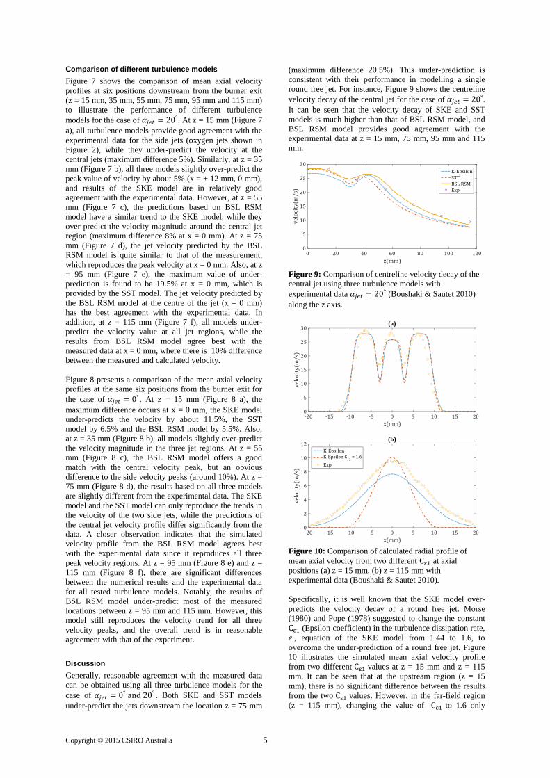
round free jet. For instance, Figure 9 shows the centreline

velocity decay of the central jet for the case of 𝛼𝑗𝑒𝑡 = 20°.

It can be seen that the velocity decay of SKE and SST

models is much higher than that of BSL RSM model, and

BSL RSM model provides good agreement with the

experimental data at z = 15 mm, 75 mm, 95 mm and 115

mm.

Figure 9: Comparison of centreline velocity decay of the

central jet using three turbulence models with

experimental data 𝛼𝑗𝑒𝑡 = 20° (Boushaki & Sautet 2010)

along the z axis.

Figure 10: Comparison of calculated radial profile of

mean axial velocity from two different Cε1 at axial

positions (a) z = 15 mm, (b) z = 115 mm with

experimental data (Boushaki & Sautet 2010).

Specifically, it is well known that the SKE model over-

predicts the velocity decay of a round free jet. Morse

(1980) and Pope (1978) suggested to change the constant

Cε1 (Epsilon coefficient) in the turbulence dissipation rate,

𝜀 , equation of the SKE model from 1.44 to 1.6, to

overcome the under-prediction of a round free jet. Figure

10 illustrates the simulated mean axial velocity profile

from two different Cε1 values at z = 15 mm and z = 115

mm. It can be seen that at the upstream region (z = 15

mm), there is no significant difference between the results

from the two Cε1 values. However, in the far-field region

(z = 115 mm), changing the value of Cε1 to 1.6 only


provides a good prediction for central jet, but under-

predicts the side jets compared with the default value of

Cε1 (1.44). Hence, this change does not improve the

simulated results in these cases.

The performance of the BSL RSM model is slightly better

than that of SST and SKE models. According to Tian,

Nathan and Cao (2015), the normal Reynolds stress in

both SKE model and SST model are assumed to be

isotropic, which reduces the prediction accuracy of a

turbulence model when dealing with turbulence flow

conditions such as jet interaction. By resolving turbulence

intensity and additional transport equations, the BSL RSM

model considers the anisotropic Reynolds stresses. Figure

11 shows the predicted normal Reynolds stress of BSL

RSM model at z = 115 mm, 𝛼𝑗𝑒𝑡 = 20° . The normal

Reynolds stress 𝜏𝑤𝑤 (ww in the figure) is predicted to be

much higher than the normal Reynolds stress 𝜏𝑣𝑣 and 𝜏𝑢𝑢 .

This may explain why the BSL RSM model has a better

performance of predicting interacting jet flow than the

other two models.

Figure 11: Predicted Reynolds stresses of BSL RSM

model at z = 115 mm with 𝛂𝐣𝐞𝐭 = 𝟐𝟎°.

CONCLUSION

The simulated results of the Baseline Reynolds Stress

(BSL RSM), the Standard k-ɛ (SKE) and the Shear-Stress-

Transport (SST) models were found to predict the

experimental data reasonably well at upstream locations of

z = 15 mm to z = 55 mm in Boushaki and Sautet (2010),

where z is the downstream distance from the burner exit.

However, all three models under-predict the measured

velocity for locations z = 75 mm to 115 mm. The best

model is the BSL RSM model, which predicts the peak

velocity magnitude (z = 75 mm) and reproduces the trend

of velocity profiles in different axial positions. Owing to

the advantage of predicting the anisotropic Reynolds

stresses, the BSL RSM model mitigates the deficiency

found in SKE and SST models. Therefore, the BSL RSM

model is expected to provide good prediction to

interacting jet flows, and it is deduced to be the preferred

type of RANS model for the turbulent flows inside the

HSRC.

ACKNOWLEDGEMENTS

The authors will acknowledge the financial support from

the Australian Research Council.

REFERENCES

BOUSHAKI, T., MERGHENI, M.A., SAUTET, J.C.,

LABEGORRE, B (2008), ''Effects of inclined jets on

turbulent oxy-flame characteristics in a triple jet burner'',

Exp. Therm. Flu. Sci., 32, 1363-1370.

BOUSHAKI, T., SAUTET, J., SALENTEY, L.,

LABEGORRE, B (2007), ''The behaviour of lifted oxy-

fuel flames in burners with separated jets'', Int. Commun.

Heat Mass, 34, 8-18.

BOUSHAKI, T. and SAUTET, J.C. (2010),

''Characteristics of flow from an oxy-fuel burner with

separated jets: influence of jet injection angle'', Exp.

Fluids, 48, 1095-1108.

CHINNICI, A. (2015), Internal Report. The University

of Adelaide, School of Mechanical Engineering.

JIN, H.G., HONG, H. (2012), ''12 - Hybridization of

concentrating solar power (CSP) with fossil fuel power

plants'', in K Lovegrove & W Stein (eds), Concentrating

Solar Power Technology, Woodhead Publishing, 395-420.

MORSE, A.P. (1980), ''Axisymmetric Turbulent Shear

Flows with and Without Swirl'', Thesis, University of

London.

NATHAN, G.J., DALLY, B., ASHMAN, P.,

STEINFELD, A., (2013), ''A hybrid receiver-combustor'',

Provisional Patent Application No. 2012/901258.,

Adelaide Research and Innovation Pty. Ltd.; 2012

[Priority Date: 29.03.2].

NATHAN, G.J., HU, E.J., DALLY, B., ALWAHABI,

Z., BATTYE, D.L., ASHMAN, P. (2009), 'A boiler

system receiving multiple energy sources'., Provisional

Patent Application No.2009/905065 [Priority Date:

19.10.09].

ORDORICA-GARCIA, G., DELGADO, A.V.,

GARCIA, A.F. (2011), ''Novel integration options of

concentrating solar thermal technology with fossil-fuelled

and CO2 capture processes'', Energy Procedia, 4, 809-816.

POPE, S.B. (1978), ''An explanation of the turbulent

round-jet/plane-jet anomaly'', AIAA. J., 16, 279-281.

STEINMANN, W.D. (2012), ''11 - Thermal energy

storage systems for concentrating solar power (CSP)

plants'', in K Lovegrove & W Stein (eds), Concentrating

Solar Power Technology, Woodhead Publishing, 362-394.

TIAN, Z.F., NATHAN, G.J., CAO, Y. (2015),

''Numerical modelling of flows in a solar–enhanced vortex

gasifier: Part 1, comparison of turbulence models'', Prog.

Comput. Fluid Dy., 15, 114-122.

cfd modelling of isothermal multiple jets … international conference on cfd in the minerals and...

Documents