cfd computations for crm using hifun

Introduction Typical grids Results Conclusions

CFD computations for Common Research

Model using the code HIFUN

Ravindra K., Nikhil Vijay Shende, N. BalakrishnanComputational Aerodynamics Laboratory,Department of Aerospace Engineering,

Indian Institute of Science, Bangalore 560012

Fourth AIAA Drag Prediction Workshop, San Antonio, TXJune 21–22, 2009

Ravindra et.al. — DPW4: CFD computations for CRM using HIFUN 1/33


Outline

1 Introduction

2 Typical grids

3 Results

4 Conclusions



Introduction

Tools employed

Grid generation for Common Research Model (CRM) iscarried out using GAMBIT and TGRID, commercialsoftwares from Fluent available at SupercomputerEducation and Research Centre (SERC), IISc.

Flow computations for CRM are performed using the codeHIFUN, a commercial software from Simulation andInnovation Engineering Solutions (SandI) available atCAd Lab, Department of Aerospace Engineering, IISc.

Postprocessing is carried out using TECPLOT available atSERC, IISc.



Features of code HIFUNHIFUN: HIgh Resolution Flow Solver on UNstructured Meshes

Algorithmic features

Unstructured cell centre finite volume methodology.

Higher order accuracy: linear reconstruction procedure.

Flux limiting: Venkatakrishnan Limiter.

Inviscid flux computation: Roe scheme.

Convergence acceleration: matrix free symmetric GaussSeidel relaxation procedure.

The viscous flux discretization: Green–Gauss theorembased diamond path reconstruction.

Eddy viscosity computation: Spalart Allmaras TM.

Parallelization: MPI.



Outline

1 Introduction

2 Typical grids

3 Results

4 Conclusions



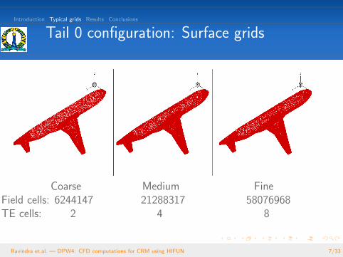
Tail 0 configuration: Surface grids

Coarse Medium FineField cells: 6244147 21288317 58076968TE cells: 2 4 8



Tail 0 configuration: Cut sectionCut section at 40 % of wing span

Coarse Medium FineBL Cells: 21 31 41

Average y+: 0.50 0.40 0.27Max y+: 0.89 0.74 0.52



Tail 0 configuration: Surface grids

← Nose

← Wing fuselage junction

← Tail fuselage junctionCoarse Medium Fine



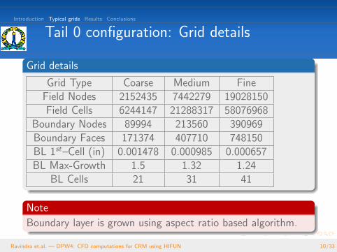
Tail 0 configuration: Grid details

Grid details

Grid Type Coarse Medium FineField Nodes 2152435 7442279 19028150Field Cells 6244147 21288317 58076968

Boundary Nodes 89994 213560 390969Boundary Faces 171374 407710 748150BL 1st–Cell (in) 0.001478 0.000985 0.000657BL Max-Growth 1.5 1.32 1.24

BL Cells 21 31 41

Note

Boundary layer is grown using aspect ratio based algorithm.



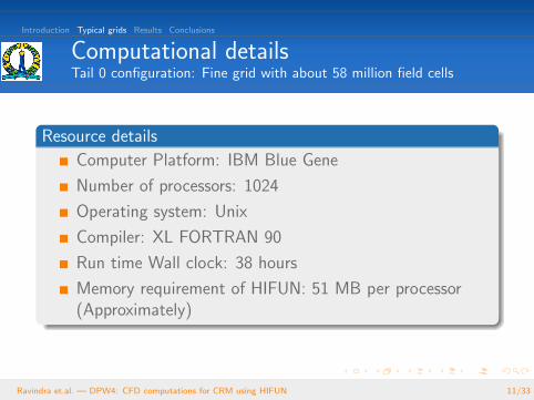
Computational detailsTail 0 configuration: Fine grid with about 58 million field cells

Resource details

Computer Platform: IBM Blue Gene

Number of processors: 1024

Operating system: Unix

Compiler: XL FORTRAN 90

Run time Wall clock: 38 hours

Memory requirement of HIFUN: 51 MB per processor(Approximately)



Outline

1 Introduction

2 Typical grids

3 Results

4 Conclusions



Outline

3 ResultsCase 1.1: Grid convergenceCase 1.2: Downwash studyCase 3 (optional): Reynolds number study



Tail 0 configuration: Pressure distributionM∞ = 0.85,Re∞ = 5.00 million,CL = 0.5± 0.001

← Overall

← WingCoarse Medium Fine

α = 2.34o α = 2.31o α = 2.3o



Tail 0 configuration: Cp distributionM∞ = 0.85,Re∞ = 5.00 million,CL = 0.5± 0.001

← Wing

← Tail



Tail 0 configuration: Drag convergenceM∞ = 0.85,Re∞ = 5.00 million,CL = 0.5± 0.001

CDo CDpr CDfr

Comments

For CDo and CDpr , ∆y = 2 drag counts and for CDfr ,∆y = 1 drag count.

Drag curves do not asymptote on fine grid.



Separation bubble: wing fuselage junctionM∞ = 0.85,Re∞ = 5.0 million,CL = 0.5± 0.001

← Grids

← BubblesCoarse Medium Fine

α = 2.34o α = 2.31o α = 2.3o



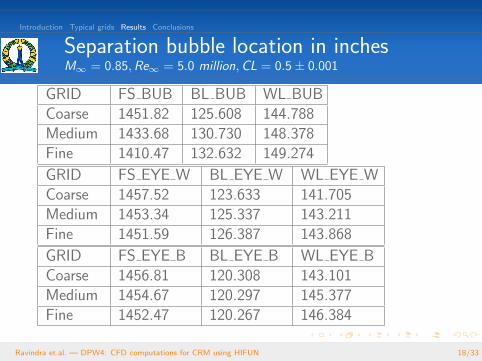
Separation bubble location in inchesM∞ = 0.85,Re∞ = 5.0 million,CL = 0.5± 0.001

GRID FS BUB BL BUB WL BUBCoarse 1451.82 125.608 144.788Medium 1433.68 130.730 148.378Fine 1410.47 132.632 149.274

GRID FS EYE W BL EYE W WL EYE WCoarse 1457.52 123.633 141.705Medium 1453.34 125.337 143.211Fine 1451.59 126.387 143.868

GRID FS EYE B BL EYE B WL EYE BCoarse 1456.81 120.308 143.101Medium 1454.67 120.297 145.377Fine 1452.47 120.267 146.384



Separation line near wing trailing edgeM∞ = 0.85,Re∞ = 5.0 million,CL = 0.5± 0.001

← Close view

← Closer viewCoarse Medium Fine

Separation line extends between the stations that are 39.71%and 84.56% of wing span.



Outline




Comparison of integrated coefficientsM∞ = 0.85,Re∞ = 5.0 million

CL CD CM



Comparison of integrated coefficientsM∞ = 0.85,Re∞ = 5.0 million

Drag polar CL v/s CM



Trim drag and downwash calculationsM∞ = 0.85,Re∞ = 5.0 million

Trim angle Trim drag Downwash



Outline




Reynolds number studyTail 0, CL = 0.5± 0.001, Mach = 0.85, Medium grid

Re Field cells BL–first spacing (in) Average y+

5.0E6 21288317 0.000985 0.4020.0E6 22802687 0.000273 0.29

Re α CLT CDT CMT

5.0E6 2.31 0.4997 0.02765 -0.0414120.0E6 2.07 0.4991 0.02264 -0.04592

Re CDP CDSF CD−CL2

PA

5.0E6 0.01695 0.01069 0.01881820.0E6 0.01434 0.00829 0.013829



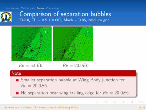
Comparison of separation bubblesTail 0, CL = 0.5± 0.001, Mach = 0.85, Medium grid

Re = 5.0E6 Re = 20.0E6

Note

Smaller separation bubble at Wing Body junction forRe = 20.0E6.

No separation near wing trailing edge for Re = 20.0E6.



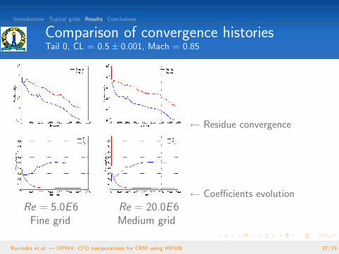
Comparison of convergence historiesTail 0, CL = 0.5± 0.001, Mach = 0.85

← Residue convergence

← Coefficients evolution

Re = 5.0E6 Re = 20.0E6Fine grid Medium grid



Outline

1 Introduction

2 Typical grids

3 Results

4 Conclusions



Concluding remarks

Conclusions

In the present work, results of RANS computations forCommon Research Model using the code HIFUN arepresented.

Unstructured hybrid grids for various configurations aregenerated using GAMBIT and TGRID.

During grid generation, except for the number of fieldcells and number of trailing edge points, the guidelinesprovided by DPW4 committee are followed.



Concluding remarks

Conclusions continued

With grid refinement, total drag shows reduction by 4–8drag counts. However, the drag curves do not asymptoteon fine grid. Hence any conclusion about the gridconvergence of drag can be drawn only after obtainingresults on extra–fine grid.

Separation bubble is seen at wing–fuselage junction andwith grid refinement it becomes more pronounced.

Separation line is seen near the trailing edge on the wingupper surface. The location and spanwise extent of theseparation line does not change with grid refinement.

For all the grids, no separation is observed on the tail.



Concluding remarks

Conclusions continued

We await the experimental results for validation ofdownwash and trim drag calculations.

For Re = 20.0E6, separation bubble seen at thewing–fuselage junction is smaller in size compared to theone seen for Re = 5.0E6.

For Re = 20.0E6, no separation is observed near wingtrailing edge.



Acknowledgments

Authors wish to thank Prof. Govindarajan, Chairman,Supercomputer Education and Research Centre (SERC), IIScfor permitting them to use IBM Blue Gene facility on apreferential queue and Mr. Kiran, System Administrator, IBMBlue Gene, for his help in the execution; but for this supportthese computations wouldn’t have been possible.

Authors also wish to thank Dr. Joseph Morrison for kindlyagreeing to make this presentation.



Thank you

Thank you

Thank you

Contact

Ravindra K.: [email protected]

Nikhil Vijay Shende: [email protected]

N. Balakrishnan: [email protected]


cfd computations for crm using hifun

Documents