cfd capabilites for hypersonic scramjet propulsive ...€¦ · data cfd ge o m figure 2: wall...

AIAA-2004-4131

CFD CAPABILITIES FOR HYPERSONIC SCRAMJET PROPULSIVE FLOWPATH DESIGN R.J. Ungewitter, J.D. Ott, V. Ahuja and S.M. Dash Combustion Research and Flow Technology, Inc. (CRAFT Tech) Pipersville, PA 18947

40th AIAA/ASME/SAE/ASEE Joint Propulsion Conference and Exhibit

11-14 July 2004 / Ft. Lauderdale, FL

CFD Capabilities for Hypersonic Scramjet Propulsive Flowpath Design

R.J. Ungewitter*, J.D. Ott*, V. Ahuja†, and S.M. Dash‡

Combustion Research and Flow Technology, Inc. (CRAFT Tech) 6210 Keller’s Church Road, Pipersville, PA 18947

Email: [email protected]

This paper discusses the status of our CFD capabilities for scramjet flow path analysis and design, as well as key enabling technologies that enhance accuracy and efficiency. A scramjet engine flow path encompasses some of the most complex aero-propulsive physics including; laminar to turbulent flow transition, complex shock interactions, and multi-species reacting chemistry. Through the judicious use of advanced modeling and adaptive procedures to ensure adequate resolution, CFD can now predict the performance characteristics of proposed engine designs. Several enhancements to the baseline modeling approach are presented and their influence is demonstrated on unit problems representative of scramjet flow paths.

Nomenclature Prt = Turbulent Prandtl Number Sct = Turbulent Schmidt Number Le = Lewis Number, Prt/Sct

Reθ = Reynolds Number based on momentum boundary layer thickness M = Mach Number k,ε = Turbulent kinetic energy, turbulent dissipation rate Tw = Temperature of wall PDE = Partial differential equation

I. Introduction sing a combination of both structured (CRAFT CFD® code) and multi-element unstructured (CRUNCH CFD® code) numerics1,2, the authors have previously evaluated the ability of CFD codes to analyze a variety of

scramjet propulsive flow paths3. Data sets from Holden and coworkers (obtained in the CUBRC /LENS shock tunnel facility) were used in this evaluation for generic, full-scale model variants of Hyper-X (Mach 10), NASP (Mach 12), and AFOSR (Mach 7.5) configurations tested at fully-duplicated flight conditions using Hydrogen fuel. The CFD evaluation study3, performed using “first-generation” CFD methodology, indicated that reasonable comparisons with nose-to-tail data sets were obtainable for run conditions for which self-ignition readily occurred without the use of ignition-aids (i.e. without Silane), as well for conditions where the ignition enhancement effect achieved could be replicated in a simplified manner. The CFD calculations performed were CPU intensive and did not implement recent modeling and numerical upgrades that enhance both accuracy and efficiency. This paper will discuss some of these newer upgrades that comprise “second-generation” CFD capabilities and will describe some basic studies.

U

Upgrades of particular relevance that will be discussed include: I. Utilization of engineering-oriented transition onset (kl model) and intermittency (λ model) models.

40th AIAA/ASME/SAE/ASEE Joint Propulsion Conference and Exhibit, 11-14 July 2004, Fort Lauderdale, Florida * Research Scientist, AIAA Member. † Research Scientist, AIAA Senior Member. ‡ Chief Scientist & President, AIAA Associate Fellow

Copyright © 2004 by the authors. Published by AIAA with permission.

American Institute of Aeronautics and Astronautics

1

These models permit addressing effects of free stream fluctuations and disturbances (angle change, trips, etc.) on transitional behavior, as well as heating and 3D effects where the transitional process is not a simple streamwise one for which purely algebraic models may be adequate.

II. Utilization of multi-element / multi-level grid adaptation. This is a requirement in fuel injection zones where combustion efficiency tends to be over-estimated

until the grid is sufficiently resolved. III. Utilization of efficient stiff chemistry methodology for ignition sensitive problems.

Using a higher-order, iterative chemical kinetic solver (in a point implicit manner) for problems where extended ignition reactions are required leads to load balancing issues that are remedied by using a “work per node” load balancing strategy.

IV. Utilization of scalar fluctuation models to extract local values of turbulent Prandtl and Schmidt numbers. LES studies for unit high speed problems indicate Lewis numbers of about 2 are reasonable for self-

similar jets, and shear layers4, but, that use of advanced models (which solve additional PDE’s for temperature/species fluctuations and dissipation rates and can calculate a local value of Prt/Sct) are needed for fuel injection regions.

V. Utilization of multi-variate optimization methods to determine geometries yielding best performance. Such techniques have been used with success to obtain optimal nozzle geometries and are being

examined to optimize combustor details (shape, injector patterns, etc). The remainder of this paper will describe the CFD methodology utilized and each of the above upgrades and its influence on solution accuracy and/or efficiency.

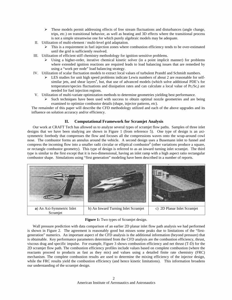
II. Computational Framework for Scramjet Analysis Our work at CRAFT Tech has allowed us to analyze several types of scramjet flow paths. Samples of three inlet designs that we have been studying are shown in Figure 1 (from reference 5). One type of design is an axi-symmetric forebody that compresses the flow and focuses all the compressions waves onto the wrap-around cowl nose. The combustor forms an annulus around the vehicle. A second design uses a Busemann inlet to funnel and compress the incoming flow into a smaller radii circular or elliptical combustor6 (other variations produce a square, or rectangle combustor geometry). This type of design is referred to as an inward turning inlet scramjet. The third type is similar to the first except that it is two-dimensional, having an inlet ramp with a high aspect ratio rectangular combustor shape. Simulations using “first generation” modeling have been described in a number of reports.

a) An Axi-Symmetric Inlet

Scramjet b) An Inward Turning Inlet Scramjet c) 2D Planar Inlet Scramjet

Figure 1: Two types of Scramjet design.

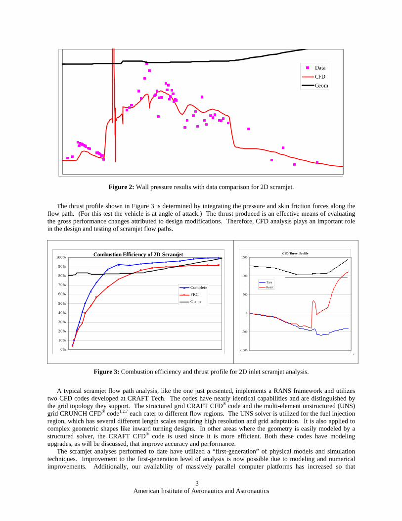
Wall pressure prediction with data comparison of an earlier 2D planar inlet flow path analysis we had performed is shown in Figure 2. The agreement is reasonably good but misses some peaks due to limitations of the “first-generation” numerics. An important aspect of the CFD analysis is the additional information (beyond pressure) that is obtainable. Key performance parameters determined from the CFD analysis are the combustion efficiency, thrust, viscous drag and specific impulse. For example, Figure 3 shows combustion efficiency and net thrust (T-D) for the 2D scramjet flow path. The combustion efficiency profiles include values based on complete combustion (where the reactants proceed to products as fast as they mix) and values using a detailed finite rate chemistry (FRC) mechanism. The complete combustion results are used to determine the mixing efficiency of the injector design, while the FRC results yield the combustion efficiency (and hence kinetic limitations). This information broadens our understanding of the scramjet design.


2

DataCFDGeom

Figure 2: Wall pressure results with data comparison for 2D scramjet.

The thrust profile shown in Figure 3 is determined by integrating the pressure and skin friction forces along the

flow path. (For this test the vehicle is at angle of attack.) The thrust produced is an effective means of evaluating the gross performance changes attributed to design modifications. Therefore, CFD analysis plays an important role in the design and testing of scramjet flow paths.

Combustion Efficiency of 2D Scramjet

0%

10%

20%

30%

40%

50%

60%

70%

80%

90%

100%

Complete

FRC

Geom

CFD Thrust Profile

-1000

-500

0

500

1000

1500

TareReact

.

Figure 3: Combustion efficiency and thrust profile for 2D inlet scramjet analysis.

A typical scramjet flow path analysis, like the one just presented, implements a RANS framework and utilizes

two CFD codes developed at CRAFT Tech. The codes have nearly identical capabilities and are distinguished by the grid topology they support. The structured grid CRAFT CFD® code and the multi-element unstructured (UNS) grid CRUNCH CFD® code1,2,7 each cater to different flow regions. The UNS solver is utilized for the fuel injection region, which has several different length scales requiring high resolution and grid adaptation. It is also applied to complex geometric shapes like inward turning designs. In other areas where the geometry is easily modeled by a structured solver, the CRAFT CFD® code is used since it is more efficient. Both these codes have modeling upgrades, as will be discussed, that improve accuracy and performance.

The scramjet analyses performed to date have utilized a “first-generation” of physical models and simulation techniques. Improvement to the first-generation level of analysis is now possible due to modeling and numerical improvements. Additionally, our availability of massively parallel computer platforms has increased so that


3

analyses with 256 (or more) processors is becoming routine, allowing for rapid turn around of nose-to-tail studies, even at higher levels of physical modeling. Table I lists two levels of modeling available for analyzing scramjet flow paths. The first level is referred to as first-generation and is the level at which all our scramjet analyses have been performed. The second level adds more advanced models and is referred to as second-generation. The improvements to the first-generation models include better transitional turbulence models, improved turbulence models, enhanced grid adaptation, a stiff chemistry solver so extended chemistry models can be utilized, and design optimization techniques that can be applied to flow path definition studies.

Table I: Scramjet Numerical Modeling Definition Models Level 1 / First-Generation

Modeling Level 2 / Second-Generation

Modeling Transitional Models Turbulence Models

Grid Adaptation Turbulent Scalar Transport

H/N/O Kinetics

Flow Path Design

Algebraic Onset/Intermittency Unified Kε

Single pass, tet/prism refinement Constant Prt, Sct

Basic H2/O2 (8 Step, 7 Species)

Trial and Error

PDE’s for onset/intermittency EASM extensions

Multi-pass, tet/prism/hex refinement Local values from PDE’s

Extended ignition (HO2, H2O2) with stiff chemistry solver

Multi-Variate Design Optimization

We are presently in the final stages of evaluating several of these second-generation models and calibrating them for use in scramjet flow paths. All improvements are discussed in following sections, except the EASM extensions, which is discussed in other publications.8,9

III. Transitional Turbulence Modeling A key physical aspect to be addressed in scramjet modeling is the transition of the flow along the fore body from

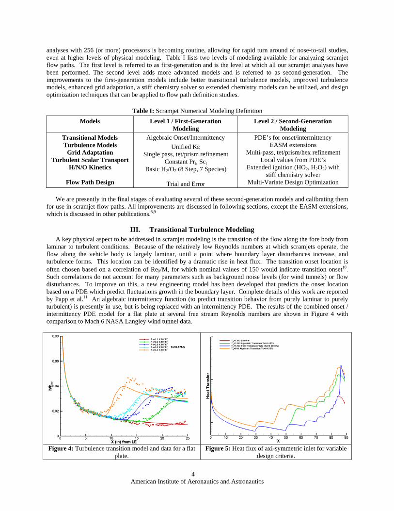
laminar to turbulent conditions. Because of the relatively low Reynolds numbers at which scramjets operate, the flow along the vehicle body is largely laminar, until a point where boundary layer disturbances increase, and turbulence forms. This location can be identified by a dramatic rise in heat flux. The transition onset location is often chosen based on a correlation of Reθ/M, for which nominal values of 150 would indicate transition onset10. Such correlations do not account for many parameters such as background noise levels (for wind tunnels) or flow disturbances. To improve on this, a new engineering model has been developed that predicts the onset location based on a PDE which predict fluctuations growth in the boundary layer. Complete details of this work are reported by Papp et al.11 An algebraic intermittency function (to predict transition behavior from purely laminar to purely turbulent) is presently in use, but is being replaced with an intermittency PDE. The results of the combined onset / intermittency PDE model for a flat plate at several free stream Reynolds numbers are shown in Figure 4 with comparison to Mach 6 NASA Langley wind tunnel data.

Figure 4: Turbulence transition model and data for a flat plate.

Figure 5: Heat flux of axi-symmetric inlet for variable design criteria.


4

The predictions show good agreement with data using free stream velocity fluctuation levels felt to be in accord with tunnel levels. The model has the ability to predict earlier transition when background fluctuations (noise level) are higher, which plays an important role when scramjet designs are transferred from ground test facilities to flight environments (low noise).

The transition onset model (with algebraic transitional blending) is demonstrated on an axi-symmetric conical forebody similar to the one shown in Figure 1a. This design has an initial 2 degree half-angle cone and increases the compression in small finite increments. The free stream Mach number is 10. Several analyses are made, varying the free stream turbulence intensity and the wall temperature. Figure 5 shows the heat flux results of the different analyses. The green curve shows heat flux based on background noise levels representative of shock tunnel test facilities and transitions at about 52”. Using negligible background noise levels similar to flight (blue line) the transition point is closer to 82”, which is near the location predicted by the Reθ/M correlation. Finally, the orange curve is the profile using a colder wall temperature. It shows transition at 42”. The variation in transition onset will have significant affects on scramjet performance. Early transition will lead to larger boundary layers, which reduce inlet recovery and thus adversely affect performance. The second-generation transition model improves our modeling capability and provides a technique to analyze more complex 3D inlet designs like the inward turning inlet.

IV. Grid Adaptation Grid adaptation is a key enabling technology needed for accurate scramjet studies at both the Level 1 and Level

2 analysis level. Our experiences in analyzing scramjet combustors has indicated a need to perform adaptation in the fuel injection region since the baseline grid does not adequately resolve the fuel/air mixing layer and thus diffusion is too rapid yielding an overly optimistic value of combustion efficiency12. CRAFT Tech has developed an advanced grid adaptation capability for the CRUNCH CFD® code which has successfully been applied to Level 1 analyses using a tetrahedral/ prism refinement scheme.

Based on work being performed, supported by the Air Force (in collaboration with Dr. Tim Baker/Princeton University), the generalized multi-element grid adaptation code, CRISP CFD®, has been further developed and enhanced to now include hexahedral elements.13 CRISP CFD® has modules for performing mesh coarsening and refinement, feature extraction and surface projection, load rebalancing, and, inter-processor communication updates. A summary of the multi-element adaptation approach used in CRISP CFD® is provided in Table II.

Table II: Multi-Element Grid Adaptation Approach

Modification of mesh according to cell topology (blocks of tets/prisms/hexes

Delaunay refinement procedure for tetrahedra

Tetrahedral regions: Delaunay refinement scheme locally

enriches the mesh Edge collapse coarsens mesh, removes

cell in benign regions of flow Edge collapse procedure for tetrahedra

Prism and Hexahedral regions: Subdivision methods with transition cells

to close hanging nodes Subdivision of interface pyramids

bridging tet/hex blocks Prism subdivision methods

Simultaneous alteration of decomposed mesh in parallel, load balancing done after modifications are complete

Hexahedral cell subdivision with transition cells


5

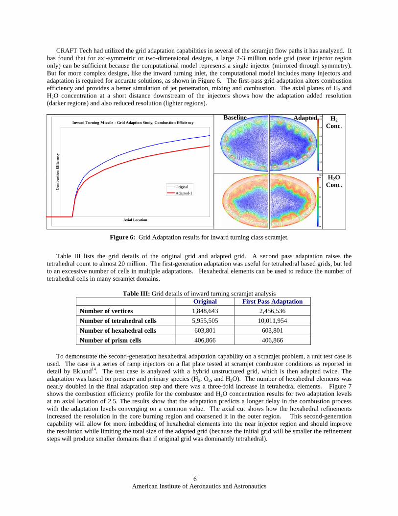
CRAFT Tech had utilized the grid adaptation capabilities in several of the scramjet flow paths it has analyzed. It has found that for axi-symmetric or two-dimensional designs, a large 2-3 million node grid (near injector region only) can be sufficient because the computational model represents a single injector (mirrored through symmetry). But for more complex designs, like the inward turning inlet, the computational model includes many injectors and adaptation is required for accurate solutions, as shown in Figure 6. The first-pass grid adaptation alters combustion efficiency and provides a better simulation of jet penetration, mixing and combustion. The axial planes of H2 and H2O concentration at a short distance downstream of the injectors shows how the adaptation added resolution (darker regions) and also reduced resolution (lighter regions).

H2 Conc. Inward Turning Missile - Grid Adaption Study, Combustion Efficiency

Axial Location

Com

bust

ion

Effic

ienc

y

OriginalAdapted-1

Baseline Adapted

H2O Conc.

Figure 6: Grid Adaptation results for inward turning class scramjet.

Table III lists the grid details of the original grid and adapted grid. A second pass adaptation raises the

tetrahedral count to almost 20 million. The first-generation adaptation was useful for tetrahedral based grids, but led to an excessive number of cells in multiple adaptations. Hexahedral elements can be used to reduce the number of tetrahedral cells in many scramjet domains.

Table III: Grid details of inward turning scramjet analysis

Original First Pass Adaptation Number of vertices 1,848,643 2,456,536 Number of tetrahedral cells 5,955,505 10,011,954 Number of hexahedral cells 603,801 603,801 Number of prism cells 406,866 406,866

To demonstrate the second-generation hexahedral adaptation capability on a scramjet problem, a unit test case is

used. The case is a series of ramp injectors on a flat plate tested at scramjet combustor conditions as reported in detail by Eklund14. The test case is analyzed with a hybrid unstructured grid, which is then adapted twice. The adaptation was based on pressure and primary species (H2, O2, and H2O). The number of hexahedral elements was nearly doubled in the final adaptation step and there was a three-fold increase in tetrahedral elements. Figure 7 shows the combustion efficiency profile for the combustor and H2O concentration results for two adaptation levels at an axial location of 2.5. The results show that the adaptation predicts a longer delay in the combustion process with the adaptation levels converging on a common value. The axial cut shows how the hexahedral refinements increased the resolution in the core burning region and coarsened it in the outer region. This second-generation capability will allow for more imbedding of hexahedral elements into the near injector region and should improve the resolution while limiting the total size of the adapted grid (because the initial grid will be smaller the refinement steps will produce smaller domains than if original grid was dominantly tetrahedral).


6

Eklund Test Case Adapted: H2O based Combustion Efficiency

0.0%

10.0%

20.0%

30.0%

40.0%

50.0%

60.0%

0.00 1.00 2.00 3.00 4.00 5.00 6.00

Original

Adapted-1

Adapted-2

Combustion Efficiency of Eklund Ramp Injector Original Grid Adapted -1 Adapted-2

Figure 7: Combustion Efficiency and Axial results for Eklund unit problem.

V. Stiff Chemistry Solver An extended H2/O2 ignition reaction mechanism that includes species such as HO2 and H2O2 is needed under

operating conditions where self-ignition is not assured. Ignition reactions are extremely stiff and have not been included in the Level 1 modeling effort because of the computational costs. A specialized multi-step, implicit solver configured to treat stiff systems of strongly coupled ODE’s has been developed and incorporated into the CRAFT Tech CFD codes15. With this solver, the computational effort required to integrate the kinetic equations over a time-step varies greatly over the solution domain, which introduces severe multi-processor load balancing issues. For example, regions of stiff chemistry may require numerous iterations to achieve a specified level of accuracy while more benign regions may only require a minimal number of iterations.

To illustrate this stiff chemistry load balancing problem, Figure 8 presents contours of OH mole fraction and normalized computational time using a stiff chemistry solver for a transverse plane in the plume of a hydrocarbon missile (which includes several of the ignition species). The OH contours (left side) show the highly convoluted reacting plume shear layer. Normalized computational time (t’) contours (right side) for the stiff chemistry solver show a wide range of time scales, ranging from zero in the free stream to large values along the reaction front in the plume shear layer. This distribution of time scales for the stiff solver in Figure 9 creates a large parallel CPU load imbalance based on standard data parallel decomposition strategy where each processor gets the same number of grid cells.

DATA PARALLELDECOMPOSITION

DYNAMIC CHEM TIMEDECOMPOSITION

DATA PARALLELDECOMPOSITION

DYNAMIC CHEM TIMEDECOMPOSITION

Figure 8: 3-D plume flow OH mole

fraction contours (left) and stiff chemistry solver normalized time

contours (right).

Figure 9: 3-D plume data parallel decomposition normalized processor time contours (left) and stiff chemistry solver

normalized time contours (right).

Figure 10: 3-D plume normalized processor time contours for data parallel

(left) and dynamic chemical time parallel decomposition strategies.

The load imbalance introduced by the stiff solver is shown in Figure 9, which again plots the chemical time

contours (right side) and the normalized processor time contours (t*) (left side) using the data parallel


7

decomposition strategy. For the processor time contours, each processor boundary is outlined for clarity. Most of the computational effort is concentrated in a handful of processors clustered around the shear layer.

To alleviate the load balancing problem seen in Figure 9, an automated dynamic load balancing strategy was developed and implemented. Within this strategy, we keep track of the node and processor timing and periodically redistribute the workload when a load imbalance tolerance criterion is violated. This algorithm modifies the processor splitting to achieve optimum load balancing based on the chemical solution time. Figure 10 presents normalized processor time contours for the same plane using the original data parallel (left side) and the new dynamic chemical time (right side) decomposition strategy. From this figure, the processor time for the chemical time strategy is nearly uniform, indicating optimal load balancing. With this new dynamic decomposition strategy, excellent load balancing can be achieved throughout a simulation using the stiff chemistry solver, thereby reducing the total CPU run time. The time saving may be substantial, reducing the computation effort by factors of 2 to 10, depending on the problem. The second-generation stiff chemistry model allows the inclusion of ignition chemistry mechanisms to the scramjet analysis process. Simulation under conditions where ignition is marginal or air chemistry is important can now be investigated and accuracy determined.

VI. Scalar Fluctuation Modeling for Variable Prt,/ Sct Modeling A strong dependence on the value of turbulent Prandtl number and turbulent Schmidt number for scramjet flow

path analyses has been identified16. The ratio of the two parameters is the Lewis number. Traditional RANS simulations relate turbulent diffusion of a scalar field to the fluctuating velocity field through a parameter, which reflects the strength of the velocity fluctuations relative to the scalar fluctuations. In the case of temperature, this parameter is the turbulent Prandtl number Prt, where the turbulent diffusivity αt is expressed as a function of the eddy viscosity µt by the relation:

t

tt Prρ

µα = (1)

In the case of species concentration, the turbulent Schmidt number provides a similar relation between the eddy viscosity and turbulent mass diffusivity. The assumption implicit in this traditional treatment is that the scalar fluctuations are proportional to the local velocity fluctuations, and if a uniform proportionality constant can be applied no further equations need to be solved. However, the value of this proportionality constant will depend on the geometry and flow field in question and it is up to the practitioner to derive this constant, preferably based on empirical data. In complex flows it is unlikely that the proportionality constant is uniform and a judgment will be required on the appropriate constant to use, most likely in the absence of empirical data. This is the approach used in Level I analyses.

To overcome the limitations for analyzing turbulence effects on scalar transport in complex geometries, a methodology within the framework of a RANS-based k-ε turbulence model has been developed to solve for fluctuating scalar quantities and relate the effect of local turbulence on scalar diffusion. For example, the variable turbulent Prandtl number model, based on the work of Nagano & Kim17 and Sommer et al.18,19 has been implemented to predict a local value of Prt, by solving for a temperature variance kT and its dissipation rate εT at each computational point. The local value of turbulent Prandlt number is then calculated from the relation

T

Tt k

kCC

Pr εελ

µ= (2)

which relates the turbulent momentum and energy time scales. CRAFT Tech has extended this framework to analyze propulsive jets20. (The kT-εT variable Prandtl number model has been further developed and will be presented in more detail in an upcoming paper by Brinckman21.) The local Prandtl number is applied along with the local turbulent eddy viscosity to develop the turbulent heat diffusivity αt according to Eq. (1).

A similar treatment may be used to derive a variable Schmidt number for fluctuating species concentration, thus providing a local feedback mechanism to the turbulent mass diffusivity. The added expense of solving transport equations for fluctuating species concentration can be avoided if a constant value of turbulent Lewis number is assumed. In this case, if the local turbulent Prandtl number is calculated as discussed above, then the turbulent Schmidt number can be inferred from the relation for Lewis number, or the opposite approach can be used.


8

Eklund Lewis Number Comparison: Combustion Efficiency (H2O Based)

0.0%

10.0%

20.0%

30.0%

40.0%

50.0%

60.0%

70.0%

0.00 1.00 2.00 3.00 4.00 5.00 6.00

Le=2.0

Le=1.0

H2O

0

Figure 11: Eklund Unit Problem with diffe

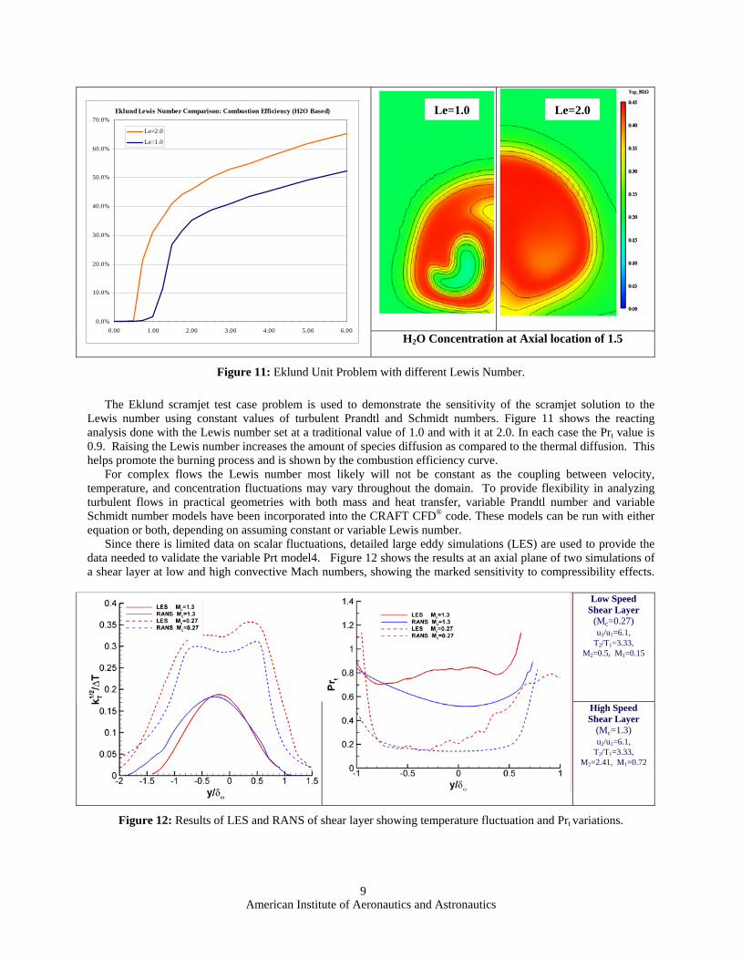
The Eklund scramjet test case problem is used to demonstrate Lewis number using constant values of turbulent Prandtl and Schanalysis done with the Lewis number set at a traditional value of 1.0 0.9. Raising the Lewis number increases the amount of species diffushelps promote the burning process and is shown by the combustion ef

For complex flows the Lewis number most likely will not betemperature, and concentration fluctuations may vary throughout theturbulent flows in practical geometries with both mass and heat trSchmidt number models have been incorporated into the CRAFT CFequation or both, depending on assuming constant or variable Lewis n

Since there is limited data on scalar fluctuations, detailed large edata needed to validate the variable Prt model4. Figure 12 shows thea shear layer at low and high convective Mach numbers, showing the

Figure 12: Results of LES and RANS of shear layer showing te

American Institute of Aeronautics an

9

Le=1.

Concentration at Axial

rent Lewis Number.

the sensitivity of the scrmidt numbers. Figure 1and with it at 2.0. In eacion as compared to the thficiency curve. constant as the coupli domain. To provide fansfer, variable Prandtl D® code. These models umber. ddy simulations (LES) a results at an axial plane marked sensitivity to c

mperature fluctuation an

d Astronautics

Le=2.0

location of 1.5

amjet solution to the 1 shows the reacting h case the Prt value is ermal diffusion. This

ng between velocity, lexibility in analyzing number and variable

can be run with either

re used to provide the of two simulations of ompressibility effects.

Low Speed Shear Layer

(Mc=0.27) u2/u1=6.1,

T2/T1=3.33, M2=0.5, M1=0.15

High Speed Shear Layer

(Mc=1.3) u2/u1=6.1,

T2/T1=3.33, M2=2.41, M1=0.72

d Prt variations.

The first LES case is done at a convective Mach number of 0.27 and the other at a higher value of 1.3 (see ref. 4). The problem was also done with a variable Prt model so as to compare the modeled Prt value to the LES value. Both the thermal fluctuations and the resulting turbulent Prandtl number are shown. Several issues become evident. First the turbulent Prandtl number is vastly different for the two flows and deviates from the traditional value of 0.9. Second the variable Prt model is able to capture the basic features of the thermal fluctuation. Scramjet injectors tend to have high convective Mach numbers so a variable Prt model would improve the numerical simulations.

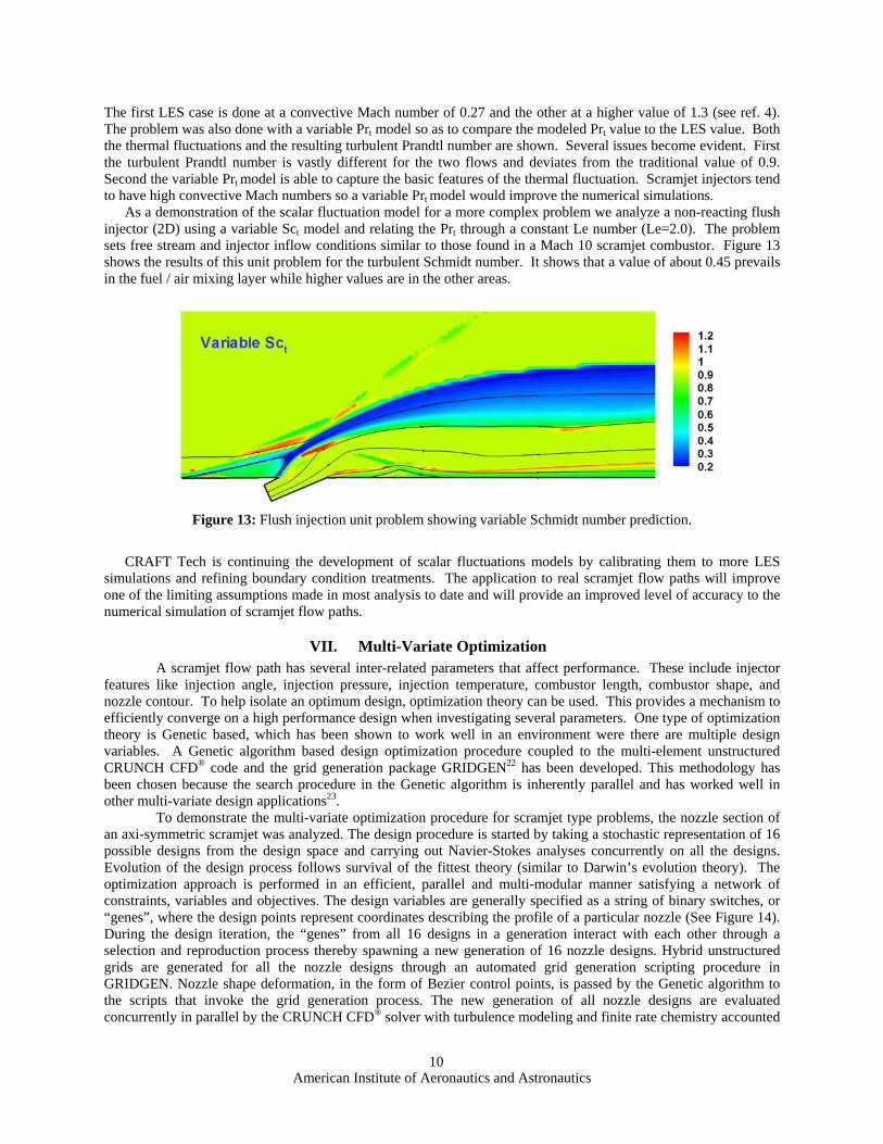
As a demonstration of the scalar fluctuation model for a more complex problem we analyze a non-reacting flush injector (2D) using a variable Sct model and relating the Prt through a constant Le number (Le=2.0). The problem sets free stream and injector inflow conditions similar to those found in a Mach 10 scramjet combustor. Figure 13 shows the results of this unit problem for the turbulent Schmidt number. It shows that a value of about 0.45 prevails in the fuel / air mixing layer while higher values are in the other areas.

Figure 13: Flush injection unit problem showing variable Schmidt number prediction.

CRAFT Tech is continuing the development of scalar fluctuations models by calibrating them to more LES

simulations and refining boundary condition treatments. The application to real scramjet flow paths will improve one of the limiting assumptions made in most analysis to date and will provide an improved level of accuracy to the numerical simulation of scramjet flow paths.

VII. Multi-Variate Optimization A scramjet flow path has several inter-related parameters that affect performance. These include injector

features like injection angle, injection pressure, injection temperature, combustor length, combustor shape, and nozzle contour. To help isolate an optimum design, optimization theory can be used. This provides a mechanism to efficiently converge on a high performance design when investigating several parameters. One type of optimization theory is Genetic based, which has been shown to work well in an environment were there are multiple design variables. A Genetic algorithm based design optimization procedure coupled to the multi-element unstructured CRUNCH CFD® code and the grid generation package GRIDGEN22 has been developed. This methodology has been chosen because the search procedure in the Genetic algorithm is inherently parallel and has worked well in other multi-variate design applications23.

To demonstrate the multi-variate optimization procedure for scramjet type problems, the nozzle section of an axi-symmetric scramjet was analyzed. The design procedure is started by taking a stochastic representation of 16 possible designs from the design space and carrying out Navier-Stokes analyses concurrently on all the designs. Evolution of the design process follows survival of the fittest theory (similar to Darwin’s evolution theory). The optimization approach is performed in an efficient, parallel and multi-modular manner satisfying a network of constraints, variables and objectives. The design variables are generally specified as a string of binary switches, or “genes”, where the design points represent coordinates describing the profile of a particular nozzle (See Figure 14). During the design iteration, the “genes” from all 16 designs in a generation interact with each other through a selection and reproduction process thereby spawning a new generation of 16 nozzle designs. Hybrid unstructured grids are generated for all the nozzle designs through an automated grid generation scripting procedure in GRIDGEN. Nozzle shape deformation, in the form of Bezier control points, is passed by the Genetic algorithm to the scripts that invoke the grid generation process. The new generation of all nozzle designs are evaluated concurrently in parallel by the CRUNCH CFD® solver with turbulence modeling and finite rate chemistry accounted


10

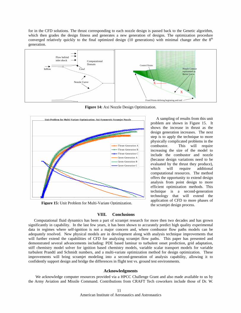
for in the CFD solutions. The thrust corresponding to each nozzle design is passed back to the Genetic algorithm, which then grades the design fitness and generates a new generation of designs. The optimization procedure converged relatively quickly to the final optimized design (10 generations) with minimal change after the 8th generation.

Nozzle Curve

Computational Domain

Flow behind inlet shock

CowlInflow

Fixed Points defining beginning and end

Nozzle Contour represented as Bezier Curve

X

X

Control Points

Figure 14: Axi Nozzle Design Optimization.

A sampling of results from this unit

problem are shown in Figure 15. It shows the increase in thrust as the design generation increases. The next step is to apply the technique to more physically complicated problems in the combustor. This will require increasing the size of the model to include the combustor and nozzle (because design variations need to be evaluated by the thrust they produce), which will require additional computational resources. The method offers the opportunity to extend design analysis from point design to more efficient optimization methods. This technique is a second-generation technology that will extend the application of CFD to more phases of the scramjet design process.

Unit Problem for Multi-Variate O ptimization: Axi-Symmetric Scramjet Nozzle

Thrust-Generation A

Thrust-Generation B

Thrust-Generation C

Geom-Generation A

Geom-Generation B

Geom-Generation C

Figure 15: Unit Problem for Multi-Variate Optimization.

VIII. Conclusions Computational fluid dynamics has been a part of scramjet research for more then two decades and has grown

significantly in capability. In the last few years, it has been shown to accurately predict high quality experimental data in regimes where self-ignition is not a major concern and, where combustor flow paths models can be adequately resolved. New physical models are in development along with analysis technique improvements that will further extend the capabilities of CFD for analyzing scramjet flow paths. This paper has presented and demonstrated several advancements including: PDE based laminar to turbulent onset prediction, grid adaptation, stiff chemistry model solver for ignition based chemistry models, variable scalar transport models for variable turbulent Prandtl and Schmidt numbers, and a multi-variate optimization method for design optimization. These improvements will bring scramjet modeling into a second-generation of analysis capability, allowing it to confidently support design and bridge the differences in flight test vs. ground test environments.

Acknowledgments We acknowledge computer resources provided via a HPCC Challenge Grant and also made available to us by

the Army Aviation and Missile Command. Contributions from CRAFT Tech coworkers include those of Dr. W.


11

Calhoon, J. Chenoweth, G. Feldman, Dr. J. Papp and Dr. K. Brinckman. Dr. Kennedy at AMRDEC also has been a valuable contributor. Their efforts and support is greatly appreciated.

References 1 Ungewitter, R.J., Dash, S.M., Papp, J., Hosangadi, A., “Design-Oriented Analysis of Scramjet Combustor Flowfield Using

Combined UNS/PNS Procedure”, 36th AIAA Joint Propulsion Conference and Exhibit, Huntsville, AL, June 17-19 2000. 2 Ungewitter, R.J., Papp, J.L., Dash, S.M., “High Fidelity Design Oriented Scramjet Propulsive Flowpath Analysis,” Paper No.

AIAA-2001-3203, 37th AIAA Joint Propulsion Conference, Salt Lake City, UT, July 8-11 2001. 3 Ungewitter, R.J., Papp, J.L., Dash, S.M., and Kennedy, K., “Structured/Unstructured RANS Simulations of Hypersonic

Scramjet Propulsive Flowpaths and Comparisons with CUBRC/LENS Test Data,” 2002 JANNAF 26th Airbreathing Propulsion Subcommitte (APS) Meeting, Sandestin, FL, April 8-12 2002.

4 Calhoon, W.H., Jr., “Heat Release and Compressibility effects on Planar Shear Layer Development,” Paper No. AIAA-2003-1273, 41st Aerospace Sciences Meeting and Exhibit, Reno, NV, Jan. 6-10 2003.

5 Curran, E.T., Murthy, S.N.B., Ed., “Scramjet Propulsion,” AIAA Progress in Astronautics and Aeronautics, Vol. 189, pg. 452. 6 Billig, F.S, Jacobsen, L.S., “Comparison of Planar and Axisymmetric Flowpaths for Hydrogen Fueled Space Access Vehicle

(Invited),” Paper No. AIAA-2003-4407, 39th Joint Propulsion Conference and Exhibit, Huntsville, AL, July 20-23 2003. 7 Hosangadi, A., Lee, R.A., York, B.J., Sinha, N., and Dash, S.M., “Upwind Unstructured Scheme for Three-Dimensional

Combusting Flows,” Journal of Propulsion and Power, Vol. 12, No. 3, pp. 494-503, May-June 1996. 8 Gatski, T.B., Jongen, T., “Nonlinear eddy viscosity and algebraic stress models for solving complex turbulent flows,” Progress

in Aerospace Sciences, 36, (2000), pp. 655-682. 9 Papp, J.L., Kenzakowski, D.C., and Dash, S.M., “Calibration and Validation of EASM Turbulence Model for Jet Flowfields,”

Paper No. AIAA-2002-0855, 40th Aerospace Sciences Meeting & Exhibit, Reno, NV, January 14-17 2002 10 Berkowitz, A.M., Kyriss, C.L., and Martellucci, A., “Boundary Layer Transition Flight Test Observations,” AIAA Paper No.

77-125, Jan. 1977. 11 Papp, J.L., Kenzakowski, D.C., and Dash, S.M., “Extensions Of A Rapid Engineering Approach To Modeling Hypersonic

Laminar To Turbulent Transitional Flows,” Abstract submitted for 43rd Aerospace Sciences Meeting and Exhibit, Reno, NV, Jan. 10-13 2005.

12 Dash, S.M, Perrell, E.R., Hosangadi, A., Ungewitter, R., et al., “Missile Flowfield Modeling Advances and Data Comparisons,” Paper No. AIAA-2000-0940, 38th Aerospace Sciences Meeting & Exhibit, Reno, NV, January 10-13, 2000.

13 Cavallo, P.A., Sinha, N., and Feldman, G.M., “Parallel Unstructured Mesh Adaptation for Transient Moving Body and Aeropropulsive Applications,” Paper No. AIAA-2004-1057, 42nd Aerospace Sciences Meeting and Exhibit, Reno, NV, January 5-8, 2004.

14 Eklund, D. R., Stouffer, S.D., Northam, G.B., “Study of a Supersonic Combustor Employing Swept Ramp Fuel Injectors,” J. of Propulsion and Power, Vol. 13, No. 6, Nov-Dec. 1997.

15 Calhoon, W.H., Jr., “High Fidelity Computational Analysis of a Hydrocarbon Threat System (U),” 27th EPTS JANNAF Meeting, Stenis, MS, May 5-9, 2003.

16 Baurle, R., Eklund, D., “Analysis of Dual-Mode Hydrocarbon Scramjet at Mach 4-8”, AIAA Paper 2001-3299, 37th SISS Joint Propulsion Conference & Exhibit, Salt Lake City, UT, July 8-11, 2001.

17 Nagono, Y. and Kim. C., “A two-equation model for heat transport in wall turbulent shear flows,” J. Heat Transfer, Vol. 110, 1988, pp. 583-589.

18 Sommer T.T., So, R.M.C., & Lai, Y.G., “A near wall two-equation model for turbulent heat fluxes,” International J. Heat and Mass Transfer, Vol. 35, No. 12, 1992, pp. 3375-3387.

19 Sommer, T.P, So, R.M.C, & Zhang, H.S., “Near-Wall Variable-Prandlt Number Turbulence Model for Compressible Flows,” AIAA Journal, Vol. 31, No. 1, 1993, pp. 27-35.

20 Chidambaram, N., Dash, S.M., and Kenzakowski, D.C., “Scalar Variance Transport in the Turbulence Modeling of Propulsive Jets,” Journal of Propulsion and Power, Vol. 17, No. 1, 2001, pp 79-84.

21 Brinckman, K.W., Kenzakowski, D.C., and Dash, S.M., “Progress in Practical Scalar Fluctuation Modeling for High-Speed Aeropropulsive Flows,” Abstract submitted for 43rd Aerospace Sciences Meeting and Exhibit, Reno, NV, Jan. 10-13 2005.

22 Gridgen, Grid Generation Software Package, Ver. 15, Pointwise, Inc., Ft. Worth, TX, 2004. 23 Ahuja, V., Hosangadi, A., and Lee, Y-T., “Shape Optimization of Multi-element Airfoils Using Evolutionary Algorithms and

Hybrid Unstructured Framework,” Paper HT-Fed2004-56374, The 2004 Joint ASME-JSME Fluids Engineering Summer Conference, Charlotte, N.C., July 11-15, 2004.


12

cfd capabilites for hypersonic scramjet propulsive ...€¦ · data cfd ge o m figure 2: wall...

Documents