cfd background (1)
DESCRIPTION
CFD backgroundTRANSCRIPT

© Integrated Environmental Solutions Ltd. 2004
CFD Background
• Purpose:
To provide more CFD background in Training / Demos
To be able to answer more of those difficult questions
To show industry standard or rule of thumb approaches to using CFD
To provide advice about what to do when things go wrong
© Integrated Environmental Solutions Ltd. 2004
CFD Background
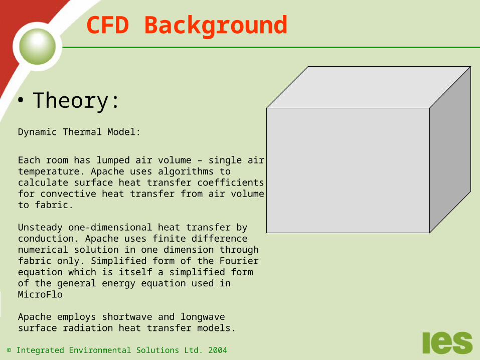
• Theory:Dynamic Thermal Model:
Each room has lumped air volume – single air temperature. Apache uses algorithms to calculate surface heat transfer coefficients for convective heat transfer from air volume to fabric.
Unsteady one-dimensional heat transfer by conduction. Apache uses finite difference numerical solution in one dimension through fabric only. Simplified form of the Fourier equation which is itself a simplified form of the general energy equation used in MicroFlo
Apache employs shortwave and longwave surface radiation heat transfer models.
© Integrated Environmental Solutions Ltd. 2004
CFD Background
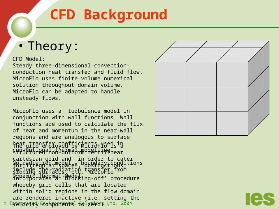
• Theory:CFD Model:Steady three-dimensional convection-conduction heat transfer and fluid flow. MicroFlo uses finite volume numerical solution throughout domain volume. MicroFlo can be adapted to handle unsteady flows.
MicroFlo uses a turbulence model in conjunction with wall functions. Wall functions are used to calculate the flux of heat and momentum in the near-wall regions and are analogous to surface heat transfer coefficients used in conventional thermal modelling.
No radiation model – boundary conditions include the radiation transfer from Dynamic Thermal Model
The grid employed by MicroFlo is a structured non-uniform rectilinear cartesian grid and in order to cater for irregular spaces, obstructions, sloping surfaces, etc. MicroFlo incorporates a ‘blocking-off’ procedure whereby grid cells that are located within solid regions in the flow domain are rendered inactive (i.e. setting the velocity components to zero) .
© Integrated Environmental Solutions Ltd. 2004
CFD Background
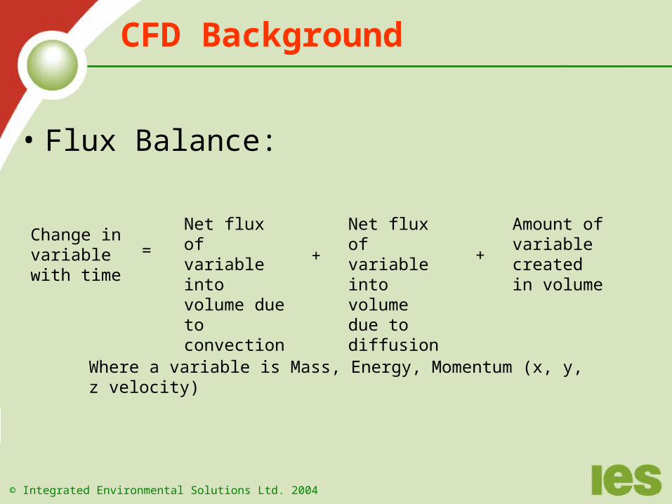
• Flux Balance:
Change in variable with time
=
Net flux of variable into volume due to convection
+
Net flux of variable into volume due to diffusion
+
Amount of variable created in volume
Where a variable is Mass, Energy, Momentum (x, y, z velocity)
© Integrated Environmental Solutions Ltd. 2004
CFD Background
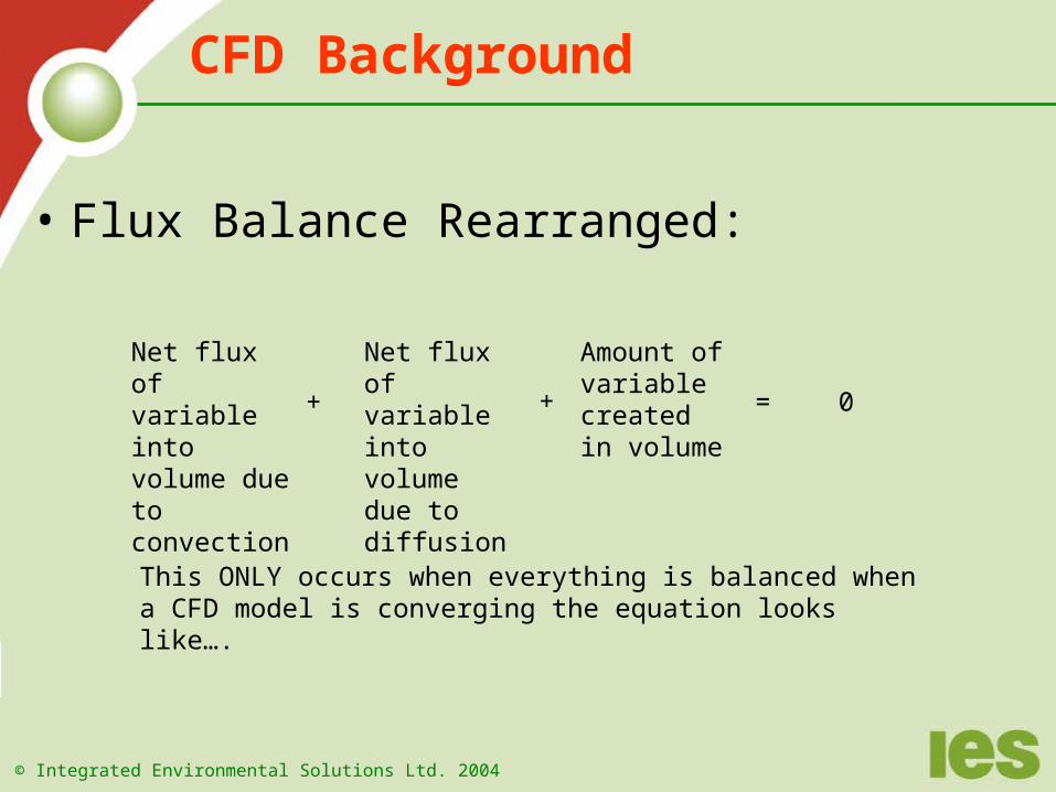
• Flux Balance Rearranged:
Net flux of variable into volume due to convection
+
Net flux of variable into volume due to diffusion
+
Amount of variable created in volume
This ONLY occurs when everything is balanced when a CFD model is converging the equation looks like….
0=

© Integrated Environmental Solutions Ltd. 2004
CFD Background
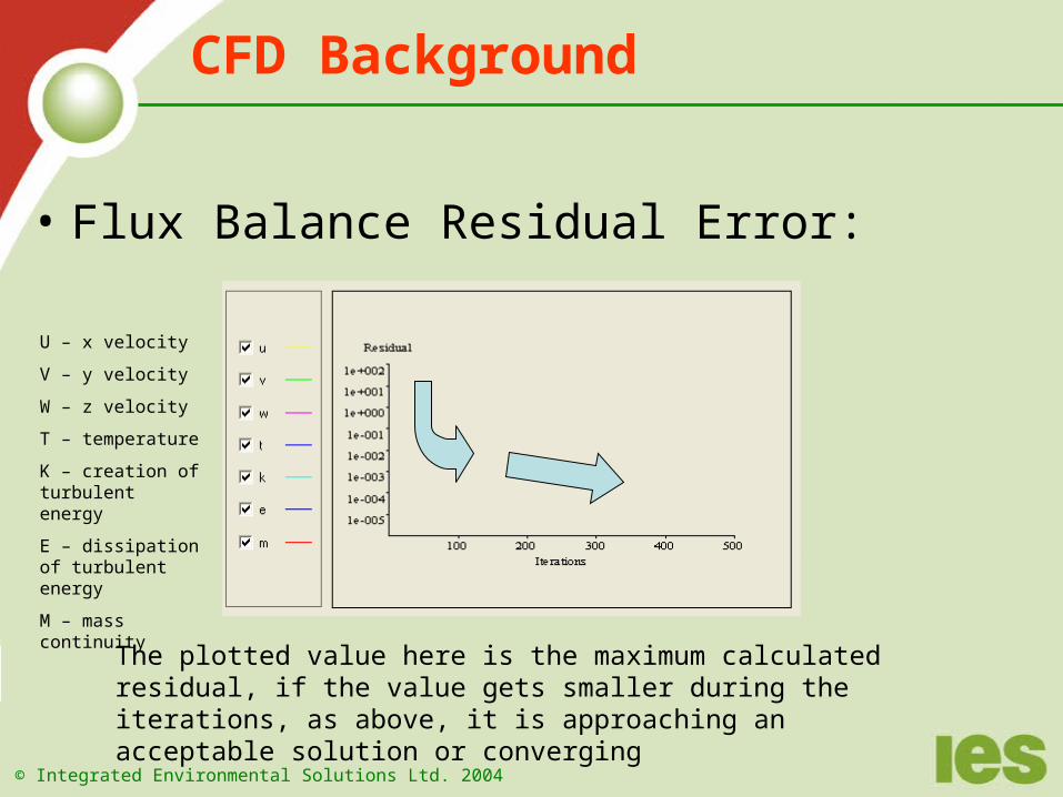
• Flux Balance Residual Error:
Net flux of variable into volume due to convection
+
Net flux of variable into volume due to diffusion
+
Amount of variable created in volume
The closer the Error to Zero the closer to a balanced flux and the closer to the TRUE answer.
CFD gets closer to the answer by iterating, that is having an initial guess – supplied by the user – and the repeatedly changing the guess until the error reduces to an acceptable level
Residual Error
=
© Integrated Environmental Solutions Ltd. 2004
CFD Background
• Flux Balance Residual Error:
The plotted value here is the maximum calculated residual, if the value gets smaller during the iterations, as above, it is approaching an acceptable solution or converging
U – x velocity
V – y velocity
W – z velocity
T – temperature
K – creation of turbulent energy
Ε – dissipation of turbulent energy
M – mass continuity
© Integrated Environmental Solutions Ltd. 2004
CFD Background
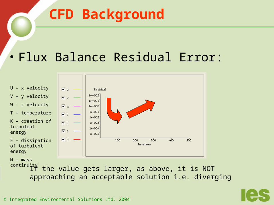
• Flux Balance Residual Error:
If the value gets larger, as above, it is NOT approaching an acceptable solution i.e. diverging
U – x velocity
V – y velocity
W – z velocity
T – temperature
K – creation of turbulent energy
Ε – dissipation of turbulent energy
M – mass continuity
© Integrated Environmental Solutions Ltd. 2004
CFD Background
• Iterations – searching for the answer:
Three issues to consider:
• Converging to the correct answer
• Diverging
• Converging to the wrong answer
© Integrated Environmental Solutions Ltd. 2004
CFD Background
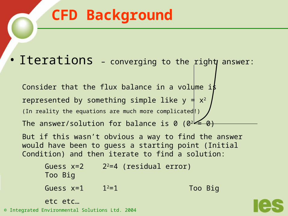
• Iterations – converging to the right answer:
Consider that the flux balance in a volume is
represented by something simple like y = x2
(In reality the equations are much more complicated!)
The answer/solution for balance is 0 (02 = 0)
But if this wasn’t obvious a way to find the answer would have been to guess a starting point (Initial Condition) and then iterate to find a solution:
Guess x=2 22=4 (residual error) Too Big
Guess x=1 12=1 Too Big
etc etc…
© Integrated Environmental Solutions Ltd. 2004
CFD Background
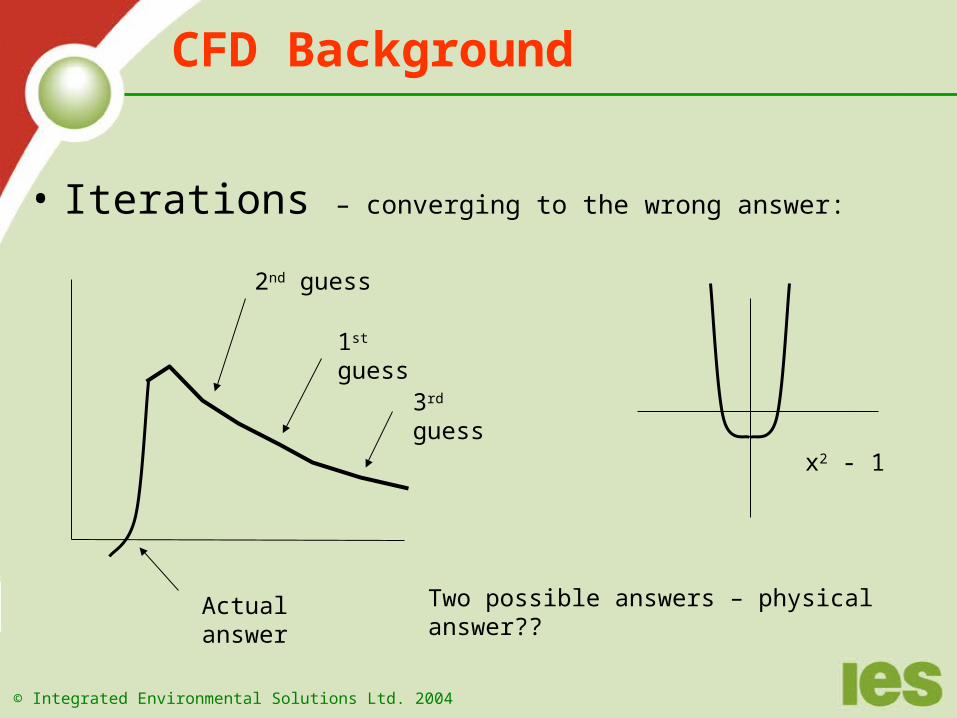
• Iterations – converging to the wrong answer:
Actual answer
2nd guess
1st guess
3rd guess
x2 - 1
Two possible answers – physical answer??
© Integrated Environmental Solutions Ltd. 2004
CFD Background
• IterationsProblems in convergence are connected with deriving the pressure field. The continuity based pressure correction equation and the resulting outer iterative scheme involves the continuing re-calculation of dependent variable coefficients. It’s this inter-linkage that causes problems, i.e. each outer iteration involves the partial solution of all of the equation sets (using inner iterative schemes) and the re-calculation of the dependent variable coefficients using the most up-to-date dependent variable values, the outer iterations being repeated until a converged solution is achieved.
Numerical procedure is very robust and is unlikely to fail.
© Integrated Environmental Solutions Ltd. 2004
CFD Background
• Good Answer?:
The results from a converged solution may not (it is unlikely) be the correct physical results how do we know?
• Check the results – hand calculations
• Is the solution dependant upon the grid - Mesh Independence Study
© Integrated Environmental Solutions Ltd. 2004
CFD Background
• Good Answer?:
Check the results:
• High velocities
• High/Low temperatures
• Large pressure differences
• Hand calc – x people @ 90W each gives a temperature rise of…
Refine the mesh in the area where there is a problem
© Integrated Environmental Solutions Ltd. 2004
CFD Background
• Good Answer?:Grid dependant:
If a mesh/grid has non regular shapes, i.e. quite long and thin volumes, or is too coarse around areas of interest it is possible that the answer is dependant upon the ‘poorness’ of the mesh.
For example, in the case of a jet being directed at a floor standing obstacle, an area of recirculation may well develop behind the obstacle but obviously this will not be revealed if the grid is too coarse in that region.
The way to check that any mesh does not have this effect is checks before the runs start (Cell Aspect Ratio) and also a grid independence study.
To do this the density of the mesh is increased globally i.e. add 20% more mesh.
Re-run the simulation and check the output is similar to the previous solution.
Practically there may not be the time!
© Integrated Environmental Solutions Ltd. 2004
CFD Background
• Questions:
What’s k-ε / constant viscosity method and when would I use one or the other?
What’s Upwind, Hybrid, and Power Law and when would I use one or the other?
What is the Maximum Cell Aspect Ratio all about then?
What’s the inner iterations/false time step and when should I change it?
What’s relaxation and when should I change it?
Termination residuals – what’s that?
© Integrated Environmental Solutions Ltd. 2004
CFD Background
• Questions:
What’s k-ε / constant viscosity method and when would I use one or the other?
k-ε (k epsilon) is a turbulence model that focuses upon the mechanisms that effect turbulent kinetic energy: the production and dissipation (destruction) of kinetic energy caused by turbulence. Calculates the turbulent viscosity. (Actually has no physical manifestation). Only applicable for fully turbulent flows
Constant viscosity method – assumes that the viscosity is constant throughout the model
© Integrated Environmental Solutions Ltd. 2004
CFD Background
• Questions:
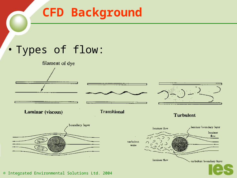
Turbulence? – fluid flows are categorised into three types of flow:
Laminar – adjacent layers of fluid slide easily over each otherTransitional – partially turbulentFully Turbulent – random and chaotic flows
Turbulent flows are used in processes to increase mixing i.e. addition of a dye to a fluid.
© Integrated Environmental Solutions Ltd. 2004
CFD Background
• Types of flow:
© Integrated Environmental Solutions Ltd. 2004
CFD Background
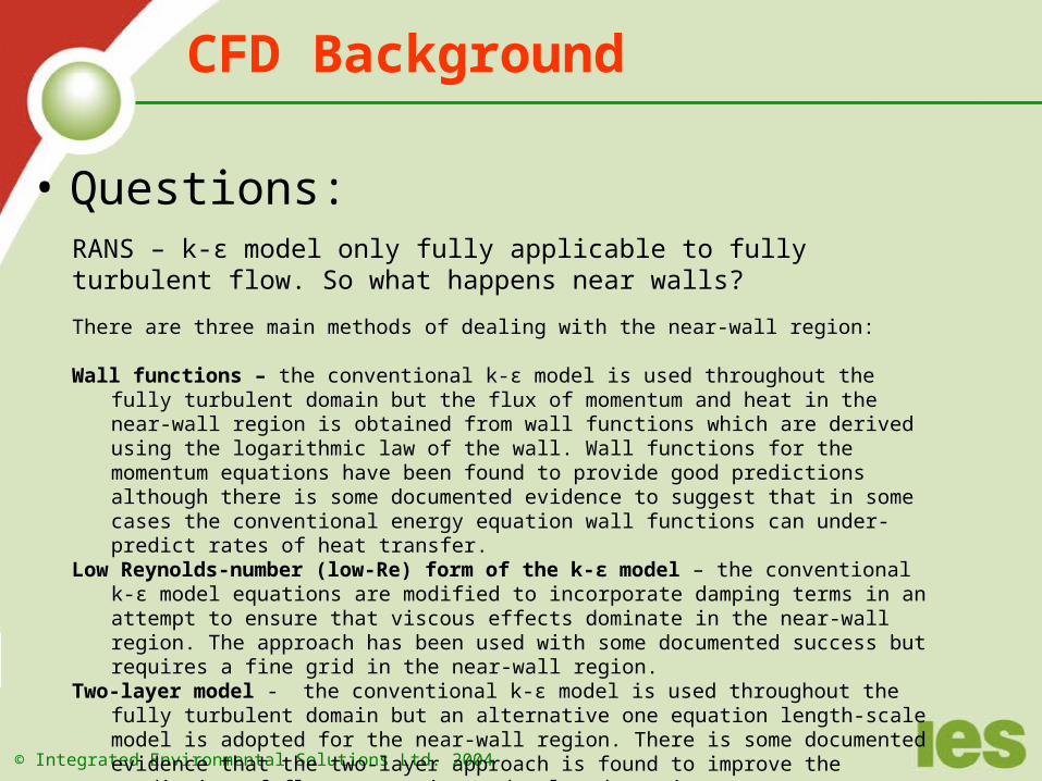
• Questions:RANS – k-ε model only fully applicable to fully turbulent flow. So what happens near walls?
There are three main methods of dealing with the near-wall region:
Wall functions – the conventional k-ε model is used throughout the fully turbulent domain but the flux of momentum and heat in the near-wall region is obtained from wall functions which are derived using the logarithmic law of the wall. Wall functions for the momentum equations have been found to provide good predictions although there is some documented evidence to suggest that in some cases the conventional energy equation wall functions can under-predict rates of heat transfer.
Low Reynolds-number (low-Re) form of the k-ε model – the conventional k-ε model equations are modified to incorporate damping terms in an attempt to ensure that viscous effects dominate in the near-wall region. The approach has been used with some documented success but requires a fine grid in the near-wall region.
Two-layer model - the conventional k-ε model is used throughout the fully turbulent domain but an alternative one equation length-scale model is adopted for the near-wall region. There is some documented evidence that the two-layer approach is found to improve the prediction of flow separation and related suction pressure prediction when used in bluff body applications (such as wind flow over buildings) when compared with the standard k-ε approach.
© Integrated Environmental Solutions Ltd. 2004
CFD Background
• Questions:Other turbulence models?
LES – Large eddy simulation.
There is documented evidence that the k-ε model can fail to accurately predict flow separation and reattachment in impingement flow conditions over bluff bodies. Specifically, turbulent intensity and suction pressure conditions over right-angled surfaces causing flow separation are not well accounted for. This failing applies to problems involving wind flow around buildings These failings have prompted interest in a new approach to turbulence modelling based on segregating the treatment of the turbulent flow into large scale and sub-grid scale. These techniques generally fall into a category of turbulence modelling called large eddy simulation (LES).
Although this method has exhibited some promise in dealing with wind flow around buildings, it is computationally much more expensive than the k-ε model and there is very little documented work available on the application of LES to internal building flow problems.
© Integrated Environmental Solutions Ltd. 2004
CFD Background
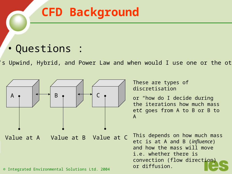
• Questions :What’s Upwind, Hybrid, and Power Law and when would I use one or the other?
A B
Value at A Value at B
These are types of discretisation
or “how do I decide during the iterations how much mass etc goes from A to B or B to A”
This depends on how much mass etc is at A and B (influence) and how the mass will move i.e. whether there is convection (flow direction) or diffusion.
C
Value at C
© Integrated Environmental Solutions Ltd. 2004
CFD Background
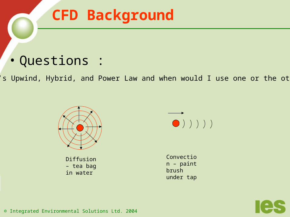
• Questions :What’s Upwind, Hybrid, and Power Law and when would I use one or the other?
Diffusion – tea bag in water
Convection – paint brush under tap
© Integrated Environmental Solutions Ltd. 2004
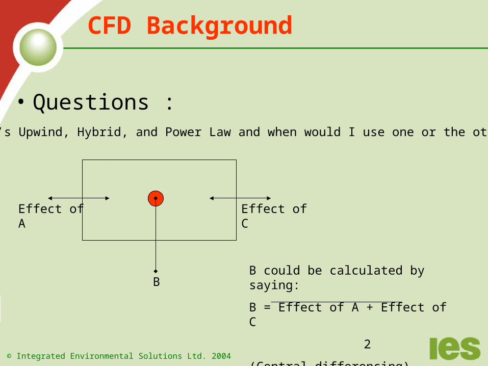
CFD Background
• Questions :What’s Upwind, Hybrid, and Power Law and when would I use one or the other?
B
Effect of A Effect of C
B could be calculated by saying:
B = Effect of A + Effect of C
2
(Central differencing)
© Integrated Environmental Solutions Ltd. 2004
CFD Background
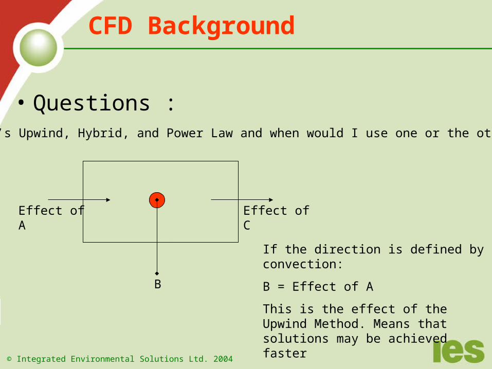
• Questions :What’s Upwind, Hybrid, and Power Law and when would I use one or the other?
B
Effect of A Effect of C
If the direction is defined by convection:
B = Effect of A
This is the effect of the Upwind Method. Means that solutions may be achieved faster
© Integrated Environmental Solutions Ltd. 2004
CFD Background
• Questions :What’s Upwind, Hybrid, and Power Law and when would I use one or the other?
Hybrid looks at the relative ratio of convection and diffusion (Pe) and chooses an appropriate method – Upwind or Central differencing.
Power Law looks around at more volume before and after the volume currently being assessed and apportions the influence of each using a power law relationship.
Both Hybrid and Power Law resort to Upwind methods when convection dominates.
Where diffusion dominates the Hybrid approach linearises the exact equations, Power Law attempts to reproduce them.
© Integrated Environmental Solutions Ltd. 2004
CFD Background
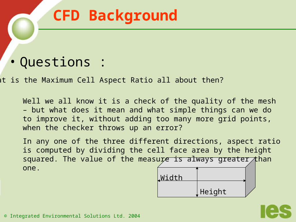
• Questions :What is the Maximum Cell Aspect Ratio all about then?
Well we all know it is a check of the quality of the mesh – but what does it mean and what simple things can we do to improve it, without adding too many more grid points, when the checker throws up an error?
In any one of the three different directions, aspect ratio is computed by dividing the cell face area by the height squared. The value of the measure is always greater than one.
Width
Height
© Integrated Environmental Solutions Ltd. 2004
CFD Background
• Questions :What is the Maximum Cell Aspect Ratio all about then?
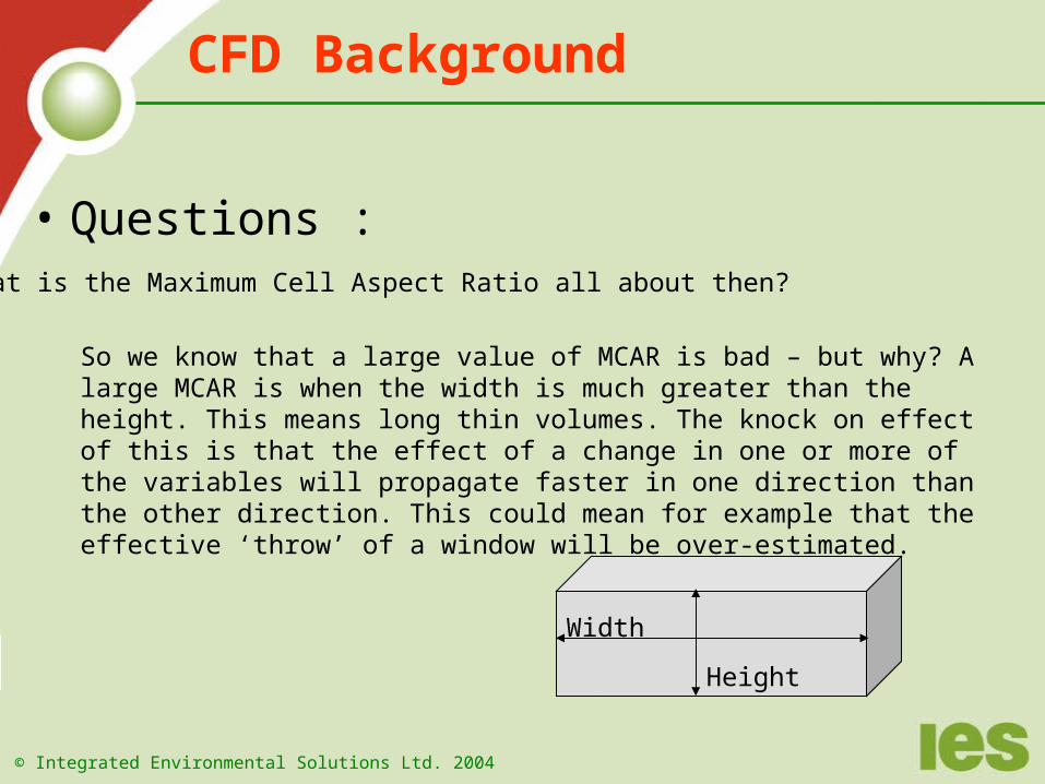
So we know that a large value of MCAR is bad – but why? A large MCAR is when the width is much greater than the height. This means long thin volumes. The knock on effect of this is that the effect of a change in one or more of the variables will propagate faster in one direction than the other direction. This could mean for example that the effective ‘throw’ of a window will be over-estimated.
Width
Height
© Integrated Environmental Solutions Ltd. 2004
CFD Background
• Questions :What’s relaxation and when should I change it?
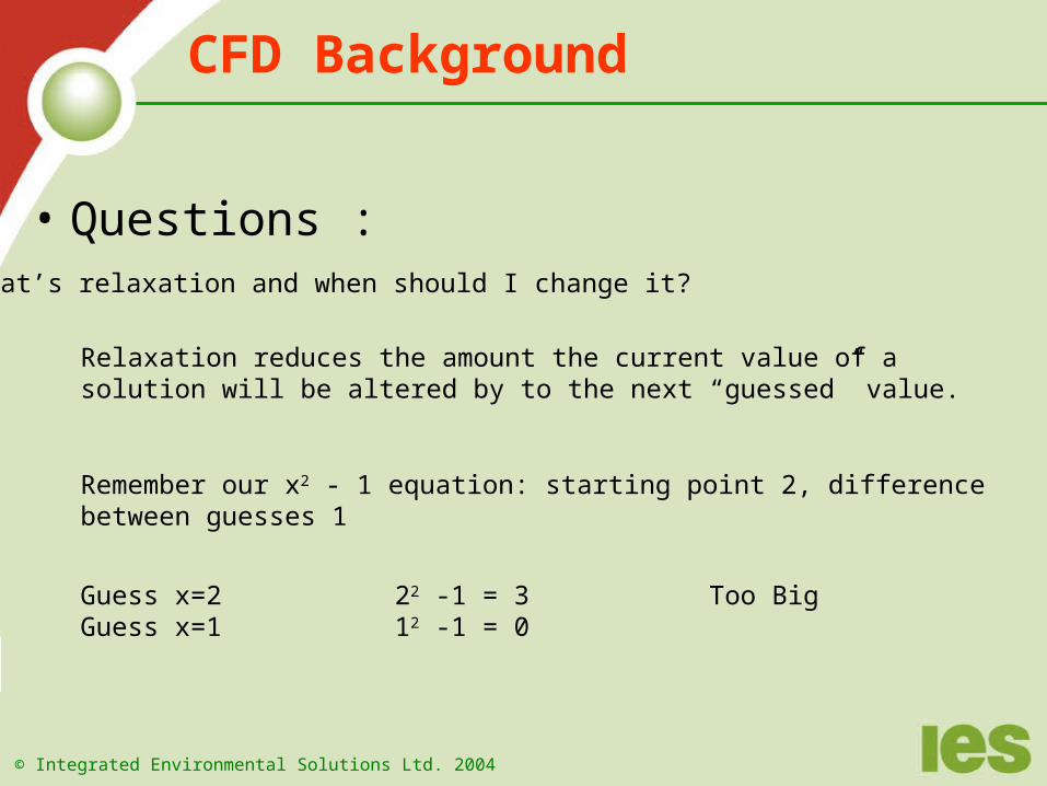
Relaxation reduces the amount the current value of a solution will be altered by to the next “guessed” value.
Remember our x2 - 1 equation: starting point 2, difference between guesses 1
Guess x=2 22 -1 = 3 Too BigGuess x=1 12 -1 = 0

© Integrated Environmental Solutions Ltd. 2004
CFD Background
• Questions :What’s relaxation and when should I change it?
What if we had started from 1.5, difference 1?
Guess x=1.5 1.52 -1 =1.25 Too Big
Guess x=0.5 0.52 -1 =-0.75 Too Small
Guess x=1.5 1.52 -1 =1.25 Too Big
Here we would be oscillating around the answer – the relaxation factor alters the step change between guesses.
i.e. an obvious relaxation here would be 0.5
New Difference between guesses = (Relaxation Factor)*(Original Difference) = 0.5 * 1
Therefore new guess x=1 (1.5-0.5) 12 – 1 = 0
© Integrated Environmental Solutions Ltd. 2004
CFD Background
• Questions :What’s relaxation and when should I change it?
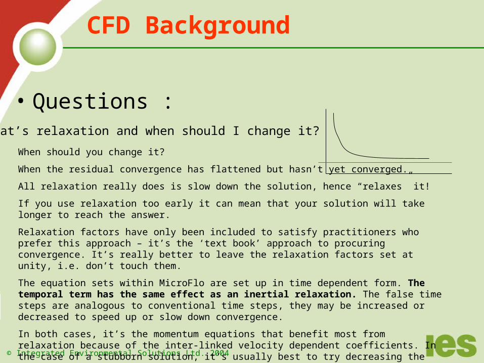
When should you change it?
When the residual convergence has flattened but hasn’t yet converged.
All relaxation really does is slow down the solution, hence “relaxes” it!
If you use relaxation too early it can mean that your solution will take longer to reach the answer.
Relaxation factors have only been included to satisfy practitioners who prefer this approach – it’s the ‘text book’ approach to procuring convergence. It’s really better to leave the relaxation factors set at unity, i.e. don’t touch them.
The equation sets within MicroFlo are set up in time dependent form. The temporal term has the same effect as an inertial relaxation. The false time steps are analogous to conventional time steps, they may be increased or decreased to speed up or slow down convergence.
In both cases, it’s the momentum equations that benefit most from relaxation because of the inter-linked velocity dependent coefficients. In the case of a stubborn solution, it’s usually best to try decreasing the velocity false time steps by consecutive factors of two.
© Integrated Environmental Solutions Ltd. 2004
CFD Background
• Questions :What’s the inner iterations/false time step and when should I change it?
Inner Iterations: number of iterations performed on each variable independently of the main iterations.False time step: the parameter that fixes the difference in values between each iterative guess.
© Integrated Environmental Solutions Ltd. 2004
CFD Background
• Questions :Termination residuals – what’s that?
Simply the point at when you consider that the solution total error is acceptably low – the default is 1 * e-005
The termination residual is the maximum calculated residual.
© Integrated Environmental Solutions Ltd. 2004
CFD Background
• Rules of Thumb:
Keep components in line in x and y and z if at all possible
Use power-law mesh spacing to increase density at areas of interest and less so in open areas.
Increase mesh in areas where there is likely to be direction changes in the flow
Sufficient mesh density in between obstacles
Avoidance of high aspect ratio
© Integrated Environmental Solutions Ltd. 2004
CFD Background
• Rules of Thumb:
Supply diffusers provide sufficient mesh density
Supply diffusers – model the actual free-area – jetting in centre of large diffuser
Check wake behind building
© Integrated Environmental Solutions Ltd. 2004
CFD Background
• Rules of Thumb:
If spaces were already joined by a hole in ModellIT and you didn’t model then the hole is counted as a wall. Remodel this using windows and Macroflo so the flow rates can be established.
Go for as regular a grid as possible.
If a solution is diverging, reduce the velocity false time steps by a factor of two and try again.
The mass residual is perhaps the best indication of convergence.
Use the cell monitor to get a better idea of convergence.
© Integrated Environmental Solutions Ltd. 2004
CFD Background
• Rules of Thumb:
Keep walls in line with the axis.
Make sure when connecting spaces that they actually join – end points
Check inlets/outlets are performing as anticipated early in the solution process to avoid wasting time converging an incorrect solution.
If possible align the predominant flow direction along one of the major grid axes. False diffusion is increased with increasingly acute angles of cell attack.
Try to ensure that the first grid point from a wall is at least 0.1-0.2m from the wall.
© Integrated Environmental Solutions Ltd. 2004
CFD Background
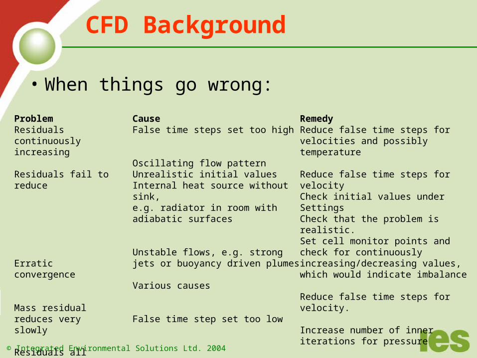
• When things go wrong:ProblemResiduals continuously increasing
Residuals fail to reduce
Erratic convergence
Mass residual reduces very slowly
Residuals all reducing steadily but very slowly
CauseFalse time steps set too high
Oscillating flow patternUnrealistic initial valuesInternal heat source without sink,e.g. radiator in room with adiabatic surfaces
Unstable flows, e.g. strong jets or buoyancy driven plumes
Various causes
False time step set too low
RemedyReduce false time steps for velocities and possibly temperature
Reduce false time steps for velocityCheck initial values under SettingsCheck that the problem is realistic.Set cell monitor points and check for continuously increasing/decreasing values, which would indicate imbalance
Reduce false time steps forvelocity.
Increase number of inner iterations for pressure
Increase false time steps

© Integrated Environmental Solutions Ltd. 2004
CFD Background
• Put an initial course mesh ~ 0.1 – 0.2 grid size everywhere• Use constant viscosity method• Run for 10 iterations check the flows and all heat sources• Run for a further 100 iterations check the solution for areas where lots of things are
happening and refine mesh if necessary• Change turbulence model to k-ε method• Refine mesh by increasing local mesh density and overall density by ~ 10 -20%• Refine mesh until solution is independent of mesh (given available time)• Use a grid of 3*3*3 cell monitors to check independence• If cell monitors are levelling out and the convergence is flattening use either
relaxation or false time steps to speed up convergence
• Standard Approach:
© Integrated Environmental Solutions Ltd. 2004
CFD Background
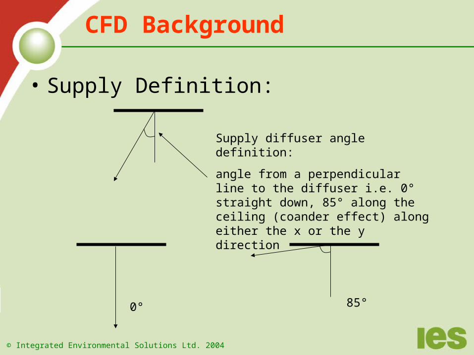
Supply diffuser angle definition:
angle from a perpendicular line to the diffuser i.e. 0° straight down, 85° along the ceiling (coander effect) along either the x or the y direction
0° 85°
• Supply Definition: