ces preferences: demands, gravity and...

CES Preferences: Demands, Gravity and VarietyNotes for Graduate International Trade Lectures

J. Peter Neary

University of Oxford

January 21, 2015

J.P. Neary (University of Oxford) CES Preferences January 21, 2015 1 / 23

Plan of Lectures

1 CES Preferences

2 The Gravity Equation

3 Measuring Gains from Variety

4 Supplementary Material


CES Preferences

Plan of Lectures

1 CES PreferencesThe CES Utility FunctionPreference for VarietyImplications of Taste for DiversityDemands





CES Preferences The CES Utility Function

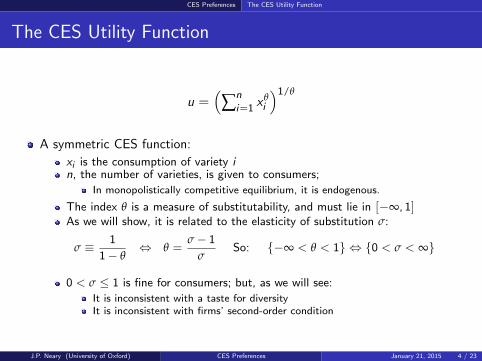
The CES Utility Function

u =(∑n

i=1xθi

)1/θ

A symmetric CES function:

xi is the consumption of variety in, the number of varieties, is given to consumers;

In monopolistically competitive equilibrium, it is endogenous.

The index θ is a measure of substitutability, and must lie in [−∞, 1]As we will show, it is related to the elasticity of substitution σ:

σ ≡ 1

1− θ⇔ θ =

σ− 1

σSo: {−∞ < θ < 1} ⇔ {0 < σ < ∞}

0 < σ ≤ 1 is fine for consumers; but, as we will see:

It is inconsistent with a taste for diversityIt is inconsistent with firms’ second-order condition


CES Preferences Preference for Variety

Preference for Variety

CES preferences imply a taste for variety:

Proof : Assume all varieties have the same price p and so are consumed inequal amounts, so total expenditure is I = npx :

xi = x = Inp ⇒ u =

(nxθ)1/θ

= n1/θx = n1

σ−1 I/pThis is the indirect utility function in symmetric equilibria

Logarithmically differentiating, with I and p fixed: [x ≡ dxx , x 6= 0]

u = 1θ n︸︷︷︸(1)

+ x︸︷︷︸(2)

= 1θ n− n = 1

σ−1 n

1 Gain at extensive margin; more than offsets:2 Loss at intensive margin

i.e., utility rises with variety for σ > 1, and by more the lower is σ.

QED


CES Preferences Implications of Taste for Diversity

Implications of Taste for Diversity

CES price index as a function of number of goods

2

0.0

0.1

0.2

0.3

0.4

0.5

0.6

0.7

0.8

0.9

1.0

0 10 20 30 40 50 60 70 80 90 100

n

P

σ = 1 0σ = 1 0σ = 5σ = 5

σ = 3σ = 3

σ = 1 . 5σ = 1 . 5

Figure 3: The Price Index and Variety

MR(high σσ)

p

x

MC

AC

B

Figure 4: Changes in the Elasticity of Substitution

MR(low σσ)

A


CES Preferences Demands

Demands

Form the Lagrangian: L ≡ uθ + λ (I − Σipixi )(uθ easier than u; yields same results: utility is ordinal not cardinal.)The term multiplied by the Lagrange multiplier λ is written such that it wouldbe positive if the constraint did not strictly bind; this ensures that λ is nevernegative.

Take the first-order conditions and manipulate to obtain:

Frisch demand functions: xi =(

λpiθ

)−σ

Relative demand functions: xixj

=(pipj

)−σ

Marshallian demand functions: xi =p−σi

Σjp1−σj

I =( piP

)−σ IP

To derive P, the true cost of living index:

Substitute Marshallian demands into u to get indirect utility function:

uθ = Σixθi =

Σip−σθi

(Σjp1−σj )

θ Iθ =

(Σjp

1−σj

)1−θI θ (since σθ = σ− 1)

⇒ V (p, I ) = IP(p)

, e (P, u) = P (p) u, P (p) ≡(

Σjp1−σj

) 11−σ


The Gravity Equation

Plan of Lectures

1 CES Preferences

2 The Gravity EquationIntroductionDigression: Newton and GravityAnderson-van WincoopAnderson-van Wincoop (cont.)Anderson-van Wincoop (cont.)Export and Import Multilateral Resistance




The Gravity Equation Introduction

The Gravity Equation

Empirically, trade volumes are well explained by simple ”gravity” equations ofthe kind: lnVjk = ln Ij + ln Ik − δdjk

Vjk is the value of exports from j to k,Ij is the value of GDP in j ,djk is the distance from j to k,δ is a parameter, often estimated to be close to 0.6.

Adding additional variables (e.g., dummies for contiguity, latitude, commonlanguage etc.) led to increased empirical success but also increasedtheoretical embarrassment:

Why does the equation work so well? How should the coefficients beinterpreted? [c.f. Leamer and Levinsohn, 1995]

Problem of interpretation came to a head with McCallum’s (AER 1995)”border puzzle”:

Controlling for GDP and distance, intra-national trade (trade between differentCanadian provinces or between different U.S. states)... is much greater than international trade (trade between a particularCanadian province and a particular U.S. state).


The Gravity Equation Digression: Newton and Gravity

Digression: Newton and Gravity

Note that Newton’s theory of gravity gives inspiration but no real guidance:

The gravitational force between two bodies (Fjk) is explained by:

Their masses (mj and mk);The distance between them djk ;G : Newton’s gravitational constant;lnFjk = lnG + lnmj + lnmk − 2 ln djk

But: the equation is exact (except for large masses when recourse must behad to Einstein’s theory of general relativity).

In any case, it does not apply to more than two bodies: the general n-bodyproblem is unsolved.


The Gravity Equation Anderson-van Wincoop

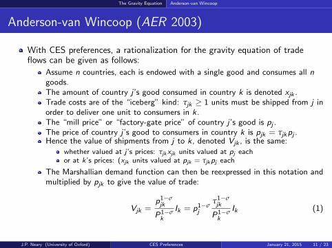
Anderson-van Wincoop (AER 2003)

With CES preferences, a rationalization for the gravity equation of tradeflows can be given as follows:

Assume n countries, each is endowed with a single good and consumes all ngoods.The amount of country j ’s good consumed in country k is denoted xjk .Trade costs are of the “iceberg” kind: τjk ≥ 1 units must be shipped from j inorder to deliver one unit to consumers in k.The “mill price” or “factory-gate price” of country j ’s good is pj .The price of country j ’s good to consumers in country k is pjk = τjkpj .Hence the value of shipments from j to k, denoted Vjk , is the same:

whether valued at j ’s prices: τjkxjk units valued at pj eachor at k’s prices: (xjk units valued at pjk = τjkpj each

The Marshallian demand function can then be reexpressed in this notation andmultiplied by pjk to give the value of trade:

Vjk =p1−σjk

P1−σk

Ik = p1−σj

τ1−σjk

P1−σk

Ik (1)


The Gravity Equation Anderson-van Wincoop (cont.)

Anderson-van Wincoop (cont.)

This is reminiscent of the gravity equation:

Depends −’ly on trade costs (for which distance is a plausible proxy);Depends +’ly on importer GDP;

But:

Exporter GDP Ij is missing;Also depends on individual goods prices pj : usually unobservable.

These problems can be overcome, and eqtn. given a GE underpinning, by invoking theGDP=Total Sales eqtn. for export country j :

Ij = Σhpjhxjh = p1−σj Σh

τ1−σjh

P1−σh

Ih (2)

Solve this for prices p1−σj and substitute into (1) to eliminate pj :

Vjk =Ij

Σhτ1−σjh

P1−σh

Ih

τ1−σjk

P1−σk

Ik =1

Σhτ1−σjh

P1−σh

θh

(τjk

Pk

)1−σ Ij Ik

IW(3)

where θh ≡ IhIW

is country h’s share in world GDP.


The Gravity Equation Anderson-van Wincoop (cont.)

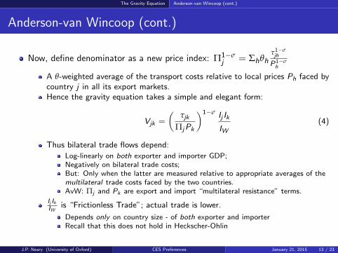
Anderson-van Wincoop (cont.)

Now, define denominator as a new price index: Π1−σj = Σhθh

τ1−σjh

P1−σh

A θ-weighted average of the transport costs relative to local prices Ph faced bycountry j in all its export markets.Hence the gravity equation takes a simple and elegant form:

Vjk =

(τjk

ΠjPk

)1−σ Ij Ik

IW(4)

Thus bilateral trade flows depend:

Log-linearly on both exporter and importer GDP;Negatively on bilateral trade costs;But: Only when the latter are measured relative to appropriate averages of themultilateral trade costs faced by the two countries.AvW: Πj and Pk are export and import “multilateral resistance” terms.

Ij IkIW

is “Frictionless Trade”; actual trade is lower.

Depends only on country size - of both exporter and importerRecall that this does not hold in Heckscher-Ohlin


The Gravity Equation Export and Import Multilateral Resistance

Export and Import Multilateral Resistance

Finally, rewrite Pk in a way that shows clearly that it is dual to Πj .

To do this, use (3) once again (with suitable changes in variables) to eliminateprices ph from the importing country’s price index Pk , which can then berewritten as a θ-weighted average of the transport costs relative to exportprices Πh faced by country k on all its imports:

P1−σk = Σhp

1−σhk = Σhp

1−σh τ1−σ

hk = ΣhIh

Σh′τ1−σhh′

P1−σh′

Ih′τ1−σhk = Σhθh

τ1−σhk

Π1−σh

Note that Πj and Pk are only defined up to a single normalization:

A 10% increase in all the Πj implies a 10% fall in all the Pk and no change inany other variables.More precisely, system is homogeneous of degree zero in Πj and P−1

k .


Measuring Gains from Variety

Plan of Lectures

1 CES Preferences


3 Measuring Gains from VarietyKonus and Sato-VartiaProof of the Sato-Vartia ResultFeenstra: Measuring the Gains from New VarietiesApplications of Sato-Vartia-FeenstraAddendum



Measuring Gains from Variety Konus and Sato-Vartia

Konus and Sato-Vartia

A different application of CES preferences.

First: Derive the true price index when variety is constant.Digression: Why do we need to derive it? Isn’t it just P?

No: P is unobservable in the realistic case of asymmetric utility:

u =

(n

∑i=1

βixθi

) 1θ

⇒ P =

(n

∑i=1

βσi p

1−σi

) 11−σ

(5)

A classic index number problem: How to find an empirical index (i.e., based onobservables) which equals (or approximates) an unobservable true index?

Solution for CES is the Sato-Vartia Index :

lnPSV ≡n

∑i=1

ωi

(ln p1

i − ln p0i

)(6)

where: ωi ≡ µiµ−1, µi ≡

s1i −s0

i

ln s1i −ln s0

i, µ ≡ ∑n

i=1 µi

In words: The SV index is a weighted geometric mean of price relatives,where the weights are the normalised logarithmic means of the budget sharesin the two periods.


Measuring Gains from Variety Proof of the Sato-Vartia Result

Proof of the Sato-Vartia Result

Demand functions xi = βσi

( piP

)−σ IP imply budget shares si = βσ

i

( piP

)1−σ

Take logs: ln si = σ ln βi + (1− σ)(ln pi − lnP)

Sum over i , with weights ωi to be determined, and take difference betweentwo periods:

lnP1 − lnP0 =n

∑i=1

ωi

(ln p1

i − ln p0i

)+

1

σ− 1

n

∑i=1

ωi

(ln s1

i − ln s0i

)(7)

Provided tastes are constant (β1i = β0

i ), the βi vanish!For the price index to equal a weighted average of log price changes, thesecond term on the right-hand side must be zero.

Hence, the true price index between the two periods equals:

lnP1 − lnP0 =n

∑i=1

ωi

(ln p1

i − ln p0i

)(8)

where: ωi ≡ µiµ−1, µi ≡

s1i −s0

i

ln s1i −ln s0

i, µ ≡ ∑n

i=1 µi


Measuring Gains from Variety Feenstra: Measuring the Gains from New Varieties

Feenstra: Measuring the Gains from New Varieties

Suppose the set of goods changes, though not fully: I = I0 ∩ I1 6= ∅Redefine the budget shares with respect to expenditure on common goods:

sti (It) = sti (I)λt where: λt ≡ ∑i∈I pti x

ti

∑i∈It pti x

ti

, t = 0, 1 (9)

Take difference in log budget shares between periods as before:

ln s1i (I1)− ln s0

i (I0) = (1− σ)[(ln p1

i − ln p0i )− (lnP1 − lnP0)

](10)

Sum this over i ∈ I only, with weights to be determined:

lnP1− lnP0 = ∑i∈I

ωi

(ln p1

i − ln p0i

)+

1

σ− 1 ∑i∈I

ωi

[ln s1

i (I1)− ln s0i (I0)

](11)

Using (9), this gives the SV result with a simple correction factor:

lnP1 − lnP0 = ∑i∈I

µiµ−1(

ln p1i − ln p0

i

)+

1

σ− 1

(ln λ1 − ln λ0

)(12)

where: µi ≡s1i (I)−s0

i (I)ln s1

i (I)−ln s0i (I)

, i ∈ I , µ ≡ ∑i∈I µi


Measuring Gains from Variety Applications of Sato-Vartia-Feenstra

Applications of Sato-Vartia-Feenstra

P1

P0=

(λ1

λ0

) 1σ−1

∏i∈I

(p1i

p0i

)ωi

(13)

Interpretation: If new varieties are important, λ1 will tend to be small

So, price index will be lowerIntuitively, a new good in period 1 has an infinite reservation price in period 0Similarly if varieties are upgraded, so b1

i > b0i for some i

Correction factor is less important the higher is σ

Ignoring new varieties matters less if they are close substitutes for existing ones

Broda-Weinstein (QJE 2006) apply this approach to U.S. imports 1972-2001

They estimate total gains from increased import varieties as 2.6 % of GDP


Measuring Gains from Variety Addendum

Addendum

Note that Feenstra (1994) defines the CES price index as

P =(

∑ni=1 bip

1−σi

) 11−σ

, i.e., bi = βσi


Supplementary Material

Plan of Lectures

1 CES Preferences



4 Supplementary MaterialSolving for CES DemandsOrigins of the CES


Supplementary Material Solving for CES Demands

Solving for CES Demands

L ≡ uθ + λ (I − Σipixi ) =n

∑i=1

βixθi + λ

(I −

n

∑i=1

pixi

)(14)

⇒ ∂L

∂xi= βi θx

θ−1i − λpi = 0 ⇒ xi =

(λpiθβi

)−σ

(15)

⇒xjxi

=

(βipjβjpi

)−σ

(16)

Solve for xj , multiply by pj and sum over j :

⇒n

∑i=1

pjxj =xi

βσi p−σi

n

∑j=1

βσj p

1−σj = I ⇒ xi =

βσi p−σi

Σjβσj p

1−σj

I (17)

⇒ xi = βσi

(piP

)−σ I

Pwhere: P ≡

[Σjβ

σj p

1−σj

] 11−σ

(18)


Supplementary Material Origins of the CES

Origins of the CES

Mathematical form developed by Hardy, Littlewood and Polya (1934)

Introduced into economics by Arrow, Chenery, Minhas and Solow (1961)

As a form for a two-factor production function

Applied to monopolistic competition by Dixit-Stiglitz (1977) and Spence(1977)

Their innovation: Making n endogenous, so allowing it to be used inmonopolistic competitionDifference between them: Spence assumed quasi-linear utility, so notapplicable to general equilibrium


ces preferences: demands, gravity and...

Documents