infolab.stanford.eduinfolab.stanford.edu/pub/cstr/reports/cs/tr/98/1601/cs-tr-98-1601.pdf · i...
TRANSCRIPT

FORMAL VERIFICATION OF PROBABILISTIC SYSTEMS
a dissertation
submitted to the department of computer science
and the committee on graduate studies
of stanford university
in partial fulfillment of the requirements
for the degree of
doctor of philosophy
By
Luca de Alfaro
December 1997

c Copyright 1998 by Luca de Alfaro
All Rights Reserved
ii

I certify that I have read this dissertation and that in my opinion
it is fully adequate, in scope and in quality, as a dissertation for
the degree of Doctor of Philosophy.
Zohar Manna(Principal Adviser)
I certify that I have read this dissertation and that in my opinion
it is fully adequate, in scope and in quality, as a dissertation for
the degree of Doctor of Philosophy.
John C. Mitchell
I certify that I have read this dissertation and that in my opinion
it is fully adequate, in scope and in quality, as a dissertation for
the degree of Doctor of Philosophy.
Rob J. van Glabbeek
I certify that I have read this dissertation and that in my opinion
it is fully adequate, in scope and in quality, as a dissertation for
the degree of Doctor of Philosophy.
Ugo Montanari
Approved for the University Committee on Graduate Studies:
iii

iv

Abstract
Methods for the formal veri�cation and speci�cation of systems are a critical tool for the development
of correct systems, and they have been applied to the design of hardware, software and control
systems. While some system properties can be studied in a non-probabilistic setting, others, such
as system performance and reliability, require a probabilistic characterization of the system. The
formal analysis of these properties is especially necessary in the case of safety-critical systems, which
must be designed to meet speci�c reliability and performance guarantees.
This dissertation focuses on methods for the formal modeling and speci�cation of probabilistic
systems, and on algorithms for the automated veri�cation of these systems. Our system models
describe the behavior of a system in terms of probability, nondeterminism, fairness and time.
The formal speci�cation languages we consider are based on extensions of branching-time tem-
poral logics, and enable the expression of single-event and long-run average system properties. This
latter class of properties, not expressible with previous formal languages, includes most of the per-
formance properties studied in the �eld of performance evaluation, such as system throughput and
average response time. We also introduce a classi�cation of probabilistic properties, which explains
the relationship between the di�erent classes of properties expressible in the proposed languages.
Our choice of system models and speci�cation languages has been guided by the goal of providing
e�cient veri�cation algorithms. The algorithms rely on the theory ofMarkov decision processes, and
exploit a connection between the graph-theoretical and probabilistic properties of these processes.
This connection also leads to new results about classical problems, such as an extension to the
solvable cases of the stochastic shortest path problem, an improved algorithm for the computation of
reachability probabilities, and new results on the average reward problem for semi-Markov decision
processes.
v

Acknowledgements
First, I would like to thank Zohar Manna, my advisor during the six years I spent at Stanford.
Under his direction, I learnt everything I know about formal methods and theoretical computer
science. Without his generosity, unconditional support and encouragement, this dissertation would
not have been possible. I would also like to thank him for creating such a friendly and stimulating
atmosphere in the research group.
I would then like to thank the members of my readings and orals committee, Rob van Glabbeek,
Tom Henzinger, Grigori Mints, John Mitchell, Ugo Montanari and Rajeev Motwani, for their time
and for their valuable comments.
Next, I would like to express my gratitude to Andrea Bianco, who brought to my attention the
topic of formal veri�cation of probabilistic systems, and with whom I wrote my �rst paper on the
subject. Working with him was an extremely enjoyable experience.
I would also like to thank Professor Arthur Veinott, who gave me very valuable advice in my
study of the theory of Markov decision processes, and who never tired of answering my questions
about references in the literature.
Many thanks also go to the other members of my research group: Nikolaj Bj�rner, Anca Browne,
Michael Col�on, Arjun Kapur, Henny Sipma and Tom�as Uribe. Phyllis Winkler, the secretary of the
group, pulled me out of several inextricable bureaucratic problems with her e�ciency and zeal.
My gratitude also goes to Angelo Ra�aele Meo, my undergraduate advisor, who �rst nurtured
my research activities, and who greatly helped me to come to Stanford.
I am also very grateful to the school teachers that had the most in uence on me; �rst among
them Adriano Attanasio, who turned me from scoundrel to attentive pupil; Giuseppe Gallione, who
taught me the beauty of elementary mathematics and axiomatic geometry, Elena Micheletti, who
taught me calculus and physics with passion and joy, and Carla Origlia, who taught me the love for
natural sciences. I am also very indebted to Gillian Sortino, from whom I learnt the language in
which I am now writing.
vi

I would also like to thank my family for their love and encouragement, for having taught me
to love mathematics and physics, and for teaching me how to think (mostly) rationally. Last, but
not least, I would like to thank my wife Fran�coise Beaufays for her incredible patience, support and
understanding, as well as for other reasons that are beyond the scope of this dissertation.
Luca de Alfaro
Stanford, California
December 1997
vii

Contents
Abstract v
Acknowledgements vi
1 Introduction 1
1.1 The Bene�ts of Formal Methods . . . . . . . . . . . . . . . . . . . . . . . . . . . . . 2
1.2 System Models . . . . . . . . . . . . . . . . . . . . . . . . . . . . . . . . . . . . . . . 3
1.3 Speci�cation Languages . . . . . . . . . . . . . . . . . . . . . . . . . . . . . . . . . . 4
1.4 Veri�cation . . . . . . . . . . . . . . . . . . . . . . . . . . . . . . . . . . . . . . . . . 5
1.5 Outline of the Dissertation . . . . . . . . . . . . . . . . . . . . . . . . . . . . . . . . . 7
1.6 How to Read This Dissertation . . . . . . . . . . . . . . . . . . . . . . . . . . . . . . 7
1.7 Chronology . . . . . . . . . . . . . . . . . . . . . . . . . . . . . . . . . . . . . . . . . 8
1.8 Related Work . . . . . . . . . . . . . . . . . . . . . . . . . . . . . . . . . . . . . . . . 8
2 Stochastic Transition Systems 17
2.1 Stochastic Transition Systems . . . . . . . . . . . . . . . . . . . . . . . . . . . . . . . 17
2.2 Application 1: Cooling a Reactor . . . . . . . . . . . . . . . . . . . . . . . . . . . . . 22
2.3 Application 2: A Token Ring Network . . . . . . . . . . . . . . . . . . . . . . . . . . 26
2.4 Concluding Remarks . . . . . . . . . . . . . . . . . . . . . . . . . . . . . . . . . . . . 32
3 Timed Probabilistic Systems 33
3.1 Markov Decision Processes and Policies . . . . . . . . . . . . . . . . . . . . . . . . . 34
3.2 Timed Probabilistic Systems . . . . . . . . . . . . . . . . . . . . . . . . . . . . . . . 40
3.3 End Components . . . . . . . . . . . . . . . . . . . . . . . . . . . . . . . . . . . . . . 44
3.4 The Stochastic Shortest Path Problem . . . . . . . . . . . . . . . . . . . . . . . . . . 50
3.5 The Maximal Reachability Probability Problem . . . . . . . . . . . . . . . . . . . . . 52
4 Basic Probabilistic Logic 67
4.1 A Brief History of Probabilistic Temporal Logics . . . . . . . . . . . . . . . . . . . . 67
viii

4.2 The Logics pTL and pTL* . . . . . . . . . . . . . . . . . . . . . . . . . . . . . . . . . 69
4.3 Checking Non-Zenoness . . . . . . . . . . . . . . . . . . . . . . . . . . . . . . . . . . 72
4.4 Model Checking for Operator P in pTL* . . . . . . . . . . . . . . . . . . . . . . . . . 73
4.5 Model Checking for Operator D in pTL and pTL* . . . . . . . . . . . . . . . . . . . 77
4.6 Complexity of pTL and pTL* Model Checking . . . . . . . . . . . . . . . . . . . . . 80
4.7 Extending the D Operator to Past Formulas . . . . . . . . . . . . . . . . . . . . . . . 82
4.8 Model Checking of Operator P in pTL . . . . . . . . . . . . . . . . . . . . . . . . . . 82
5 Speci�cation of Long-Run Average Properties 86
5.1 A Motivational Example . . . . . . . . . . . . . . . . . . . . . . . . . . . . . . . . . . 87
5.2 GPTL and GPTL*: Augmenting the Logics With Experiments . . . . . . . . . . . . 92
5.3 A Classi�cation of Probabilistic Properties . . . . . . . . . . . . . . . . . . . . . . . . 99
5.4 Expressive Power of Experiments . . . . . . . . . . . . . . . . . . . . . . . . . . . . . 101
6 Veri�cation of Long-Run Average Properties 103
6.1 Model-Checking Algorithms for GPTL and GPTL* . . . . . . . . . . . . . . . . . . . 104
6.2 Towards the Correctness Proof: Relation Between r, w and R, W . . . . . . . . . . . 109
6.3 Decomposition in End Components . . . . . . . . . . . . . . . . . . . . . . . . . . . . 112
6.4 MDP Transformation . . . . . . . . . . . . . . . . . . . . . . . . . . . . . . . . . . . 115
6.5 Reduction to Semi-Markov Optimization Problems . . . . . . . . . . . . . . . . . . . 121
6.6 Computing the Maximum and Minimum Values of J . . . . . . . . . . . . . . . . . . 128
6.7 The Correctness Proof . . . . . . . . . . . . . . . . . . . . . . . . . . . . . . . . . . . 137
6.8 Average Reward of Semi-Markov Decision Processes . . . . . . . . . . . . . . . . . . 140
7 Stochastic Shortest Path and Related Problems 148
7.1 The Non-Negative SSP Problem . . . . . . . . . . . . . . . . . . . . . . . . . . . . . 149
7.2 The Non-Positive SSP Problem . . . . . . . . . . . . . . . . . . . . . . . . . . . . . . 153
7.3 Proof of the Results for Non-Negative SSP . . . . . . . . . . . . . . . . . . . . . . . . 154
7.4 Proof of the Results for Non-Positive SSP . . . . . . . . . . . . . . . . . . . . . . . . 157
7.5 The Minimum Expected Total Cost Problem . . . . . . . . . . . . . . . . . . . . . . 159
8 Fairness 164
8.1 An Overview of Fairness . . . . . . . . . . . . . . . . . . . . . . . . . . . . . . . . . . 165
8.2 Probabilistic Fairness . . . . . . . . . . . . . . . . . . . . . . . . . . . . . . . . . . . . 165
8.3 Time Divergence and Admissible Policies . . . . . . . . . . . . . . . . . . . . . . . . 170
8.4 Probabilistic Logics for Fairness: FPTL and FPTL* . . . . . . . . . . . . . . . . . . 171
8.5 Model-Checking Algorithms for FPTL and FPTL* . . . . . . . . . . . . . . . . . . . 174
8.6 Complexity of FPTL and FPTL* Model Checking . . . . . . . . . . . . . . . . . . . 182
8.7 Correctness Proof of Model-Checking Algorithms . . . . . . . . . . . . . . . . . . . . 184
ix

9 Veri�cation of Stochastic Transition Systems 196
9.1 Translation of STSs into TPSs . . . . . . . . . . . . . . . . . . . . . . . . . . . . . . 197
9.2 Translation and Informal Semantics . . . . . . . . . . . . . . . . . . . . . . . . . . . 200
9.3 Speci�cation and Veri�cation of Stochastic Transition Systems . . . . . . . . . . . . 204
9.4 A Highway Commuter Example . . . . . . . . . . . . . . . . . . . . . . . . . . . . . . 206
9.5 Concluding Remarks . . . . . . . . . . . . . . . . . . . . . . . . . . . . . . . . . . . . 209
Bibliography 211
x

Chapter 1
Introduction
Some systems can be designed in such a way that they are guaranteed to behave correctly under all
circumstances, short of a total breakdown of the system or of its physical environment. For example,
it is possible to design integrated circuits or write some computer programs in such a way that they
will perform exactly as intended, if the power supply is present and the computer is not physically
damaged.
On the other hand, for many types of systems this guarantee of correctness cannot be achieved,
either because it would be impractically expensive, or because the system includes intrinsically
unreliable components. Examples of these systems include telecommunication systems and computer
networks, distributed systems built over these networks, and complex software-controlled physical
systems such as industrial plants, electrical power stations and transportation systems.
When a system cannot be guaranteed to exhibit the desired behavior under all circumstances,
it becomes important to characterize the likelihood of undesirable behaviors. For these systems,
the concept of unconditional correctness is substituted by bounds on the probability that certain
behaviors occur.
Even for systems whose correctness can be unconditionally guaranteed, the study of system
performance relies on a probabilistic model of the system and its load. In fact, the term system
performance commonly refers to the long-run average time required by a system to perform given
tasks, such as message delivery or response to a query. These long-run averages can be computed
on the basis of the probabilistic models.
This dissertation presents languages for the formal speci�cation of performance and reliability
properties of probabilistic systems, and algorithms for the automated veri�cation of these proper-
ties on �nite-state systems. What distinguishes this dissertation from previous work in the area
is the broader range of systems and properties covered. We consider timed systems whose behav-
ior is characterized by probability, nondeterminism, fairness and time; among them are systems
whose execution model extends that of generalized stochastic Petri nets with the introduction of
1

2 CHAPTER 1. INTRODUCTION
nondeterminism and transitions with unspeci�ed delay distributions.
The languages for formal speci�cation that we present extend the expressive capabilities of ex-
isting languages by allowing the expression of long-run average properties of systems. This class of
properties includes many basic performance measures considered in the �eld of performance modeling
and evaluation, such as system throughput and average response time. Along with this extension,
we present a classi�cation of probabilistic properties of systems, which explains the relationship
between the di�erent types of properties discussed in the dissertation.
The algorithms for the automated veri�cation of �nite-state systems rest on the theory of dynamic
programming and optimal control, as well as on results from automata theory. In particular, the the-
ory of Markov decision processes played a central role in the development of the algorithms. Several
algorithms depend on a new approach to the study of Markov decision processes, based on a joint
analysis that combines graph-theoretical and probabilistic methods. Aside from the development of
the algorithms, this approach leads to the solution of problems on Markov decision processes that
had resisted previous analysis, such as the non-negative and the non-positive cases of the stochastic
shortest path problem, and the characterization of the relation between two optimization criteria for
semi-Markov decision processes.
1.1 The Bene�ts of Formal Methods
The study of system performance and reliability has so far been carried out mostly without the use
of formal methods. The motivations for the application of formal methods to these problems can be
summarized as follows.
Precise speci�cation languages. A formal approach o�ers a language in which one can express
with precision complex system speci�cations. Most system properties relating to reliability and
performance have so far been expressed using a mixture of natural language and numbers. While this
is adequate for simple properties, the precise speci�cation of di�erent scenarios of malfunctioning
can become rather complex, and the precision of a formal language is thus bene�cial. Similarly,
while an informal approach is adequate for the speci�cation of simple performance indices, a formal
language makes it possible to de�ne in a precise way complex performance criteria and measures.
Complete coverage. While simulation methods can produce accurate estimates of reliability and
performance indices for many instances of purely probabilistic systems, they fare less well for systems
in which nondeterminism is present. In fact, for purely probabilistic systems it is possible to use
the probabilistic structure of the system to estimate the accuracy of performance indices computed
by repeated simulation. In presence of nondeterminism, however, these accuracy estimates are
substituted by the weaker notion of coverage, similarly to the case of hardware and software testing.
Without using formal methods, complete coverage is hard or impossible to achieve for systems in

1.2. SYSTEM MODELS 3
which probability and nondeterminism coexist, and incomplete coverage does not provide a reliable
measure of con�dence towards the satisfaction of design requirements.
Common framework for the study of correctness, reliability and performance proper-
ties. The study of reliability and performance properties often relies on a prior analysis of the cor-
rectness of the system under consideration. The use of formal methods o�ers a common framework
in which one can study system correctness, performance and reliability, facilitating the interchange
of information between the di�erent types of properties.
1.2 System Models
In this dissertation, we model the behavior of systems in terms of probability, nondeterminism,
fairness and time. Probability enables the modeling of system components with unreliable or proba-
bilistic behavior, and it is an essential element in the study of reliability and performance properties.
Nondeterminism enables the modeling of unknown scheduling mechanisms, and it can be used as a
replacement for more accurate probabilistic models in the construction of system approximations.
Fairness, jointly with nondeterminism, enables the modeling of unknown (but non-zero) probabili-
ties, and it is a widely used ingredient in the modeling of reactive systems. Time is used to specify
waiting-time distributions for the system transitions, and it is an essential element for the evaluation
of system performance.
We present two di�erent models for probabilistic systems: a high-level model that enables a con-
cise and readable description of systems, and a low-level model to which the veri�cation algorithms
can be applied.
The high-level model is that of stochastic transition systems (STSs). Stochastic transition sys-
tems are a probabilistic extension of �rst-order transition systems. The transitions can either be
immediate, in which case they are taken as soon as they become possible, or they can have an
associated probability distribution of waiting times. This probability distribution can either be ex-
ponential or unspeci�ed. The choice of transition is also subject to fairness requirements. Once a
transition is taken, its e�ects are described in terms of both probability and nondeterminism. The
execution model of stochastic transition systems thus extends that of generalized stochastic Petri
nets with the introduction of nondeterminism and unspeci�ed delay distributions.
Our low-level computational model is that of timed probabilistic systems (TPSs), and is based
on Markov decision processes. Markov decision processes generalize Markov chains by associating to
each state a set of possible actions. Each state-action pair is associated with a probability distribution
for the successor state. The behavior of a Markov decision process consists in an in�nite alternation
of states and actions: at each state, an action is selected nondeterministically; the corresponding
probability distribution is then used to choose the following state.

4 CHAPTER 1. INTRODUCTION
A TPS is a Markov decision process in which to each state-action pair is associated the ex-
pected time elapsed at the state when the action is chosen. Again, it is possible to specify fairness
requirements for the choice of the actions.
The relation between STSs and TPSs is similar to the relation between a �rst-order transition
system and its underlying state-transition graph: the �rst provide a concise and compositional
language for system modeling, while the second provides the structure to which the model-checking
algorithms can be applied. TPSs are a more general computational model than STSs, and in fact
it is possible to automatically translate an STS into its corresponding TPS. This translation is part
of our veri�cation methodology, since the veri�cation algorithms we present can be applied only to
TPSs.
1.3 Speci�cation Languages
The languages for the formal speci�cation of probabilistic systems that we present in this disserta-
tion are extensions of the branching-time temporal logics CTL and CTL*. The languages extend
the expressive power of CTL and CTL* by enabling the expression of two types of probabilistic
properties: single-event properties and long-run average properties.
1.3.1 Single-Event Properties
Single-event properties refer to the probability with which a system behavior satis�es a temporal
logic formula, or to the expected time with which it reaches a speci�ed set of states. These properties
owe their name to the fact that they involve the occurrence of a single event (satisfying a formula,
or reaching a set of states). In a Markov chain, the veri�cation of these properties involves the
computation of the reachability probability or the expected �rst-passage time for particular subsets
of states of the chain.
The speci�cation of single-event properties relies on two logical operators: an operator P that
enables to express bounds on the probability of satisfying temporal formulas, and an operator D
that enables to express bounds on the expected time to reach speci�ed sets of states. The class
of properties expressible with these two operators includes several reliability properties, and some
performance ones.
1.3.2 Long-Run Average Properties
Long-run average properties refer to the long-run average outcome or duration of speci�c patterns
that are repeated in�nitely often along a behavior. In a Markov chain, the veri�cation of these
properties involves the computation of the steady-state distribution of the closed recurrent classes
of the chain.

1.4. VERIFICATION 5
The speci�cation of long-run average properties relies on experiments, which are related to the
tests of process algebra. Experiments are small labeled graphs that can be used to specify behavior
patterns of interest, such as the request for a resource followed by either a grant or a refusal. Unlike
tests, experiments are meant to be repeated in�nitely often along a behavior of the system. Two
logical operators, �P and �D, enable the speci�cation of the long-run average outcome and duration
of experiments, respectively.
Long-run average properties include most classical performance measures of a system, such as
its average response time and throughput, as well as several reliability measures. Unlike single-
event properties, these properties could not be speci�ed with previous formal languages, and their
consideration is one of the novelty claims of this dissertation.
1.3.3 Classi�cation of Probabilistic Properties
The study of single-event and long-run average properties leads to a classi�cation of probabilistic
properties of systems. Properties are classi�ed along the two axes of probability vs. expected time,
and single-event vs. long-run average. This classi�cation is shown in Table 1.1, along with the logical
operators used to specify each class of properties, and examples of properties belonging to each class.
The speci�cation style we adopt is based on the speci�cation of bounds for these performance
and reliability measures: for example, we can write a formal speci�cation requiring that the average
system response time is below a speci�ed upper bound.
1.4 Veri�cation
Our choice of system models and speci�cation languages has been guided by the goal of providing
e�cient algorithms for system veri�cation. By e�cient algorithms, we mean algorithms having
polynomial time-complexity in the size of the encoding of the transition graph corresponding to the
system. The algorithms provide either a positive answer to the veri�cation problem, or information
that characterizes the system behaviors that violate the speci�cation. The algorithms can be applied
to �nite-state probabilistic systems: while in�nite-state systems can also be analyzed through the
use of abstractions and approximations, their study is beyond the scope of this dissertation.
The algorithms are based on the theory of Markov decision processes, and on results from the
theory of automata on in�nite words. In particular, the algorithms rest upon a connection, developed
in this dissertation, between the probabilistic analysis of Markov decision processes and their graph-
theoretical structure. This connection is useful not only for the design of the veri�cation algorithms,
but also in providing new results on classical problems in the theory of Markov decision processes.
Among these results are improved algorithms for the computation of reachability probabilities,
as well as extensions to the solvable cases of the stochastic shortest path problem. The extension
consists in algorithms for the solution of non-negative and non-positive instances of the stochastic

6 CHAPTER 1. INTRODUCTION
PROBABILITY TIME
Probability Expectedof events reachability time
SINGLE-
EVENTP D
What is the probability of reach-
ing deadlock from an initial state?
From a \good" state, what is the
expected time to failure?
Long-run average Long-run averageoutcome duration
LONG-RUN
AVERAGE
�P �D
How often are messages followed
by acknowledge?
What is the system's average re-
sponse time?
Table 1.1: Classi�cation of probabilistic properties discussed in this dissertation. For each of thefour classes of properties, we list also the logical operator used to specify them, as well as an informalexample of a typical property belonging to the class.

1.5. OUTLINE OF THE DISSERTATION 7
shortest path problem, and has in turn led to improved algorithms for the non-negative case of the
minimum expected total cost problem. Another result obtained in this dissertation is the proof of
the equivalence of two alternative optimization criteria for semi-Markov decision processes, closing
a problem that was open for more than two decades.
1.5 Outline of the Dissertation
The presentation of our methodology for the study of probabilistic systems begins in Chapter 2
with the introduction of stochastic transition systems (STSs), our high-level model for probabilistic
systems. In the same chapter, we also overview the probabilistic temporal logics introduced later in
the dissertation, and we present some examples of system modeling and speci�cation.
Chapter 3 introduces our low-level system models, timed probabilistic systems (TPSs), closely
related to Markov decision processes. The chapter develops the connection between the graph-
theoretical and probabilistic properties of these models, and it describes two optimization problems:
the stochastic shortest path problem and the maximum reachability probability problem.
Our simplest probabilistic temporal logics are introduced in Chapter 4, along with their model-
checking algorithms. These logics are extensions of the branching-time logics CTL and CTL*, and
can express single-event probabilistic properties. The speci�cation of long-run average properties is
the subject of Chapter 5. The chapter introduces experiments, and it presents probabilistic logics
that can express bounds on the long-run average outcome or duration of experiments. The model-
checking algorithms for these logics are presented in Chapter 6, along with their correctness proof.
Chapter 6 also discusses optimization problems for semi-Markov decision processes.
Chapter 7 presents new results on the stochastic shortest path problem. The results are needed
for subsequent model-checking algorithms, and are also of independent interest.
Chapter 8 extends our speci�cation and veri�cation methods to probabilistic systems with fair-
ness. The chapter introduces our notion of fairness, called probabilistic fairness, and compares it
with previous notions of fairness for probabilistic systems. The chapter then presents probabilistic
logics and model-checking algorithms for systems with fairness.
Chapter 9 completes the presentation of our formal veri�cation methodology by providing a
translation from STSs to TPSs. The translation enables the use of the logics and model-checking
algorithms of Chapters 3{8 for the speci�cation and veri�cation of the system models presented in
Chapter 2.
1.6 How to Read This Dissertation
There are three ways of reading this dissertation, depending on whether the reader is interested pri-
marily in formal veri�cation of probabilistic systems, in dynamic programming and optimal control,

8 CHAPTER 1. INTRODUCTION
or in both. Those who are interested in both topics can read this dissertation in linear order.
Those whose main interest is the formal veri�cation of probabilistic systems can start with
Chapters 2, 3, 4 and 5. They can then read the �rst section of Chapter 6, and from there continue
with Chapters 8 and 9.
Those whose main interest is the theory of Markov decision processes can start from Chapter 3.
From there, there are two alternatives. If they are interested in semi-Markov decision processes,
they have no alternative but to proceed through Chapters 5 and 6. Otherwise, they can skip these
two chapters and go directly to Chapter 7, which deals with extensions to the stochastic shortest
path and expected total cost problems.
Throughout the dissertation we have denoted with (z) the sections that contain detailed proofs
and arguments that are only used in few occasions; these sections can be skipped at a �rst reading,
if so desired.
1.7 Chronology
The results of Chapter 4 and, to some extent, Chapter 3, have been presented in Bianco and de Alfaro
[BdA95] and de Alfaro [dA97]. The remainder of this dissertation consists of previously unpublished
results.
1.8 Related Work
In this section we present an overview previous work in formal modeling and veri�cation of prob-
abilistic systems, mentioning also areas of other disciplines whose results have been used in this
dissertation.
1.8.1 Markov Decision Processes and Probabilistic Automata
Our low-level computational model for probabilistic systems is provided by Markov decision pro-
cesses, enriched with additional structure. Markov decision processes were introduced by Bellman
[Bel57] and Howard [How60], and have been the subject of much research in Operations Research
and Economics. Among the many books that have since been written on them, we referred most
often to the ones by Derman [Der70], Puterman [Put94] and Bertsekas [Ber87, Ber95]. Other books
on this topic are by Ross [Ros70a], Howard [How71], Heyman [HS82], Heyman and Sobel [HS84b],
and Tijms [Tij86]. Puterman [Put94] gives an extensive bibliography on Markov decision processes.
Bertsekas and Tsitsiklis [BT91] present several results on the stochastic shortest path problem.
These results were mentioned in Chapter 3, and extended in Chapter 2.
The complexity of solving optimization problems on Markov decision processes has been consid-
ered in Papadimitriou and Tsitsiklis [PT87], which compare the complexities under nondeterminism
1.8. RELATED WORK 9
alone and under nondeterminism with probability, and by Littman et al. [LDPK95]. The complexity
of the policy improvement methods under various assumptions are discussed by Melekopoglou and
Condon [MC94].
Markov decision processes are closely related to probabilistic automata, introduced by Rabin
[Rab63]. By identifying the controls of Markov decision processes with the inputs of probabilistic
automata, the two computational models are almost identical. They di�er, however, in the way they
are used: [Rab63] studies which sequences of inputs are accepted by probabilistic automata under
various acceptance conditions; the work on Markov decision processes is aimed instead at identifying
control policies that maximize or minimize given functionals. In this dissertation, the controls (or
inputs) are used to model nondeterminism, and we study the e�ect of nondeterminism on quantities
related to system performance and reliability: our point of view is thus closer to that of Markov
decision processes.
Several related models that include both probability and nondeterminism have been presented
in the computer science literature. Some of these models are the concurrent Markov chains of
Vardi [Var85], the probabilistic �nite-state programs of Pnueli and Zuck [PZ86], the NP systems of
Wang and Larsen [WL92] and the probabilistic automata of Segala and Lynch [SL94] and Segala
[Seg95a, Seg95b].
1.8.2 Logics of Programs and Probabilistic Dynamic Logics
Some of the early work in the study of probabilistic models of computation was done in the framework
of logics of programs and of dynamic logics.
Kozen [Koz79] presents two alternative semantics for probabilistic programs. One of the se-
mantics represents programs as functions on measurable spaces; the other represents programs as
operators on linear Banach spaces of measures. The relationship between these semantics and the
ordered domains of Scott and Strachey [SS71] is also discussed.
Ramshaw [Ram80] proposes Hoare-style rules for probabilistic programs, and applies them to
the study of some algorithms.
The study of probabilistic dynamic logic began with Reif [Rei80], in which the program operators
include probabilistic choice, and the tests can specify lower bounds on the probability of success.
Axiomatizations for the resulting logics are discussed. Later, Feldman and Harel [FH82] present an
extended probabilistic dynamic logic, and improve on the results of [Rei80] by proving decidability
relative to the theory of second-order arithmetic.
Kozen [Koz83] presents a dynamic logic on probabilistic models. The logic is based on an arith-
metic semantics, rather than a truth-functional one: propositions generalize measurable functions,
programs correspond to real-valued functions, and the modal constructors are function transformers;
the satis�ability relation returns a satisfaction probability. [Koz83] presents a small-model property

10 CHAPTER 1. INTRODUCTION
theorem and a polynomial-space decision procedure for the logic. Feldman [Fel83] presents a propo-
sitional and decidable version of the logic of [FH82]; the decidability result is proved by reduction
to �rst-order real-number theory.
Huth and Kwiatkowska [HK97] propose a probabilistic mu-calculus. The structure on which the
mu-calculus is evaluated includes nondeterminism, and the logical connectives are given a fuzzy-
logic semantics. For example, denoting with eP (A) the fuzzy \probability" of event A, the rule for
conjunction is eP (A^B) = maxf0; eP (A)+ eP (B)� 1g. As in [Koz83], the truth-functional semantics
of formulas is replaced by an arithmetic semantics in terms of probability intervals; the choice of the
fuzzy semantics leads to a simpli�cation of the computational procedure to evaluate the intervals on
a given structure.
A related line of research consists in considering programs as probabilistic predicate transformers.
Hart, Sharir and Pnueli [HSP84] model programs as Markov chains, and propose a veri�cation style
for the input-output relations of programs based on the use of probabilistic intermediate assertions.
Morgan, McIver and Seidel [CM96] extend the predicate-transformer approach to systems including
nondeterminism, in part based on a relational model of probabilistic computation proposed by He et
al. [HMS96]. The proposed speci�cation languages have a Hoare-like syntax, extended to probability
and nondeterminism.
1.8.3 Temporal Logics: Qualitative Veri�cation
Given a probabilistic system, the term qualitative veri�cation refers to the problem of determining
whether formulas of a given speci�cation language hold with probability 1 over the system. A
considerable amount of work has been done on this subject.
Lehman and Shelah [LS82] present three temporal logics evaluated on Markov chains. The logics
di�er for the class of Markov chains on which they are evaluated: di�erent classes of chains lead
to di�erent axiomatizations. The three classes of chains are �nite chains, bounded chains (in which
all non-zero transition probabilities are bounded from below by a non-zero constant), and in�nite
chains. They discuss linear-time temporal logics whose formulas hold i� they are satis�ed with
probability 1 by a behavior of the chain, and they provide axiomatizations for these logics.
Hart, Sharir and Pnueli [HSP82, HSP83] study systems consisting of a set of Markov chains that
execute concurrently. The scheduling mechanism is assumed to be fair but is otherwise arbitrary.
[HSP82] present a set of conditions that characterize when the system converges with probability 1
to a given set of states. The conditions are independent of the exact values of the transition probabil-
ities. The relation between probabilistic and fair choice in the study of qualitative system properties
is discussed for the �rst time. [HSP82, HSP83] also introduce K-ergodic sets, which are in some way
similar to our end components. The conditions that ensure convergence are also related to some
algorithms discussed in this dissertation.
Pnueli [Pnu83] presents a proof system that enables to verify whether a linear-time temporal

1.8. RELATED WORK 11
logic formula holds with probability 1 over a system. Again, the system is modeled as the parallel
composition of Markov chains. The concept of extreme fairness is introduced, as an approximation
of the fairness properties resulting from choices in which each outcome has non-zero probability. A
simpler concept of fairness, state fairness, is also described. This notion is the predecessor of the
notions of fairness described in Vardi [Var85] and later in Kwiatkowska and Baier [KB96].
Hart and Sharir [HS84a] continue the line of research of [LS82] by introducing branching-time
temporal logics to be interpreted on structures that are Markov chains. They distinguish two logics,
depending on whether the chains are �nite or bounded, and they provide decision procedures and
axiom systems for the resulting logics. This work has then been extended by Hart and Sharir [HS86].
Vardi [Var85] considers system modeled as Markov chains and concurrent Markov chains; the
latter are closely related to Markov decision processes, with the addition of state fairness. The
paper presents algorithms for verifying whether these systems satisfy linear-time temporal logic
speci�cations with probability 1. The proposed algorithm relies on automata-theoretic constructions,
and it is perhaps the �rst algorithm in a line of research that led to the algorithm for the model
checking of operator P described in Chapter 4.
Pnueli and Zuck [PZ86], and later [PZ93], consider the problem of verifying whether a probabilis-
tic system satis�es with probability 1 a speci�cation. The speci�cation is written in the temporal
logic RTL, which contains all past temporal operators, and the future temporal operators 2 (al-
ways) and 3 (eventually): the future operators U (until) is not present in RTL. The probabilistic
system is described by a set of states and transitions; each transition can be taken in one of several
modes, to which are associated mode probabilities. The system models are thus related to those
of [Var85]. The algorithms presented by [PZ86, PZ93] are of single exponential time-complexity
in the size of the speci�cation, unlike those of [CY88]: the lower complexity is due to the use of
RTL as speci�cation language, instead of full temporal logic. Pnueli and Zuck [PZ93] also introduce
�-fairness, a notion of fairness that accounts precisely for the properties of a probabilistic �nite-state
system, once the speci�c values of the transition probabilities are abstracted away. Thus, �-fairness
is an improvement on the concept of extreme fairness of [Pnu83]. The system models proposed in
[PZ86, PZ93] were in uential in the development of our stochastic transition systems.
Courcoubetis and Yannakakis [CY88] consider systems modeled either as Markov chains or as
concurrent Markov chains, and present algorithms to check whether a linear-time temporal formula
holds with probability 1 over such models. The algorithm they propose for Markov chains improves
on previous algorithms, and has time-complexity polynomial in the size of the system and exponential
in the size of the formula. On concurrent Markov chains, the proposed algorithms have time-
complexity polynomial in the size of the description of the system, and doubly exponential in the
size of the temporal formula. They prove that these complexities are lower bounds, thus showing
the optimality of their algorithms. The lower bound results proved in this paper are the source of
all the lower bounds cited in this dissertation. An extended version of this work has been presented

12 CHAPTER 1. INTRODUCTION
in [CY95].
Courcoubetis and Yannakakis [CY90] study the problem of maximizing the reward of a Markov
decision process, given a reward structure speci�ed by a set of omega-automata. This problem is
related to the problem of computing the maximum and minimum probabilities with which a linear-
time temporal formula holds over a system behavior. The proposed algorithm, related to those of
[CY88], can therefore be used to solve the model-checking problem for operator P in our logics, in
absence of fairness. In this dissertation we presented an alternative algorithm, based on the complete
rather than partial determinization of an omega-automaton. This complete determinization can be
performed with the algorithm described in Safra [Saf88, Saf92].
Alur, Courcoubetis and Dill [ACD91] introduce real-time probabilistic systems, which consist
of a �nite set of states and a �nite set of transitions. To each transition is associated a delay
distribution, which can either be geometrical, or have �nite-support; the model of time is discrete,
i.e. the domain of time is taken to be the set of non-negative integers. The paper presents algorithms
for verifying that real-time probabilistic systems satisfy with probability 1 speci�cations written in
the real-time temporal logic TCTL [ACD90]. These results have been later extended by [ACD92] to
continuous-time systems and speci�cations encoded by timed automata [AD90]. The system models
of [ACD91, ACD92] have been in uential in the development of our stochastic transition systems.
1.8.4 Temporal Logics: Quantitative Veri�cation
Given a probabilistic system, the term quantitative veri�cation refers to the problem of determining
the probability with which a system satis�es a speci�cation, or more generally to the problem of
verifying speci�cations that involve the numerical values of probabilities and expectations. Using
temporal logics for the quantitative speci�cation and veri�cation of probabilistic systems is the
approach taken in this dissertation. The previous work in this area has been described in Section 4.1.
1.8.5 Veri�cation of Randomized Systems
Lynch, Saias and Segala [LSS94], as well as Pogosyants and Segala [PS95], propose methods for prov-
ing time-bound properties of randomized distributed algorithms. The veri�cation of these properties
is carried out in a natural proof style, but in fact the methods of [PS95] lend themselves to a certain
degree of automation. The completeness of these methods, which are proposed for in�nite-state
systems, is not discussed.
Segala [Seg95b] presents the computational model of probabilistic automata, which are related
to Markov decision processes, albeit the notation is fairly di�erent. Real-time system are modeled
by probabilistic timed automata, in which an additional set of actions represents the passing of time.
For these systems, [Seg95b] proposes a veri�cation approach that can be used to verify properties
related to the probability of behaviors, the expected time to events, or the probability of meeting
deadlines.
1.8. RELATED WORK 13
In the proposed approach, the proof that a system satis�es a speci�cation is constructed in
a natural proof style, in which lemmas and theorems are proved at will about the system. The
methodology proposed is semi-formal, and it does not rely on a �xed set of inference rules. Facts
about simulation relations, coin lemmas and other constructs are freely used in the course of the
proof. This approach is to be contrasted with others that rely on a �xed set of inference rules and
proof methods, such as the one developed by Manna and Pnueli [MP95] for fair transition systems.
The lack of �xed inference rules makes for a fairly general veri�cation framework in which complex
systems can be studied. On the other hand, this freedom results in a lack of guidance in the process
of proof construction, and no completeness results have been presented for this informal approach.
The proposal of [Seg95b] seems thus to be better suited to the study of randomized algorithms
than to the veri�cation of reliability and performance properties of systems, not least since long-run
average properties are not dealt with.
1.8.6 Process Algebras for Performance Modeling
Process algebras have been proposed as a compositional and high-level modeling language for the
description of Markovian performance models.
G�otz, Herzog and Rettelbach [GHR93] propose the process algebra TIPP, and discuss its use for
performance modeling. Subsets of TIPP can be translated into continuous-time Markov chains, that
can then be studied with the usual methods of performance evaluation.
Gilmore and Hillston [GH94] and Hillston [Hil95, Hil96] introduce the process algebra PEPA,
which provides a concise and compositional modeling language for timed probabilistic systems.
Systems described in PEPA can be automatically translated in continuous-time Markov chains,
to which the usual performance evaluation algorithms can be applied. Donatelli, Ribaudo and
Hillston [DRH95] compare this approach with that based on stochastic Petri nets, and Ribaudo
[Rib95] presents a translation from PEPA into Petri Nets. The proceedings [Pro ] contain further
contributions to the use of process algebras as modeling languages for performance evaluation.
Bernardo, Donatiello and Gorrieri [BDG94a] introduce Markovian Process Algebra (MPA), a
stochastic process algebra in which actions can be either immediate, or have an exponential delay
distribution. The choice between immediate actions is mediated by priorities. Actions are further
divided into active and passive, depending on whether they determine the timing of synchronous
actions when the composition of systems is computed. Two semantics are de�ned for this algebra:
one is an interleaving operational semantics, the other is a Markovian semantics de�ned by transla-
tion into continuous-time Markov chains. A third semantics, de�ned by translation into Generalized
Stochastic Petri Nets, is presented in [BDG94b, BDG95]. Bernardo, Busi and Gorrieri [BBG95]
introduce stochastic contextual nets, which extend GSPN with passive transitions and contextual
arcs, and de�ne a semantics for EMPA based on a translation into stochastic contextual nets. The

14 CHAPTER 1. INTRODUCTION
advantage of this semantics, compared to the one de�ned by translation into GSPN, is that the re-
sulting nets can be considerably smaller. Once the MPA description of a system is translated into a
Markov chain, the performance of the system can be studied with the usual methods of performance
analysis. Bernardo and Gorrieri [BG96] propose extended Markovian process algebra EMPA, closely
related to MPA.
1.8.7 Stochastic Petri Nets
Much of the work in the performance evaluation of timed systems relies on the formalism of stochastic
Petri nets, introduced by Natkin [Nat80], Molloy [Mol81, Mol82] and Symons [Sym80]. Balbo [Bal95]
provides an overview of the origins and of the developments of this �eld. The proceedings of [Pet ]
are devoted to the use of Petri nets for the modeling and evaluation of system performance. Our
stochastic transition systems are in part inspired by generalized stochastic Petri nets, introduced
by Ajmone Marsan, Balbo and Conte [ABC84], and widely used in the performance evaluation of
distributed computing systems. The recent book by Ajmone Marsan et al. [ABC+94] is devoted to
this approach to performance modeling.
Ciardo, Muppala and Trivedi [CMT91] introduce GSPN reward models, which are GSPN with
additional labels that specify a reward structure. Speci�cally, a reward is associated to each mark-
ing, and an instantaneous reward is associated to each transition. A GSPN reward model can be
translated into a continuous time Markov chain with an associated reward structure. Performance
parameters such as the long-run average reward can be computed on this structure using the stan-
dard methods of Markov-chain analysis.
The modeling and expressive capabilities of GSPN reward models are similar to the capabilities of
the methods presented in this dissertation, except that the system models we consider also include
nondeterminism, fairness, and transitions with unspeci�ed delays. Due to these extensions, our
systems require radically di�erent analysis methods: our methods trade the simplicity of Markov-
chain analysis with the modeling power of nondeterminism, fairness, and unspeci�ed delays.
1.8.8 Testing, Simulation and Process Algebras
Several notions of testing preorders, simulation and bisimulation have been introduced for proba-
bilistic processes, inspired by the corresponding notions for non-probabilistic processes. Larsen and
Skou [LS89, LS91] propose languages to encode tests for probabilistic processes, and introduce a
notion of bisimulation that respects testing equivalence. They also present a probabilistic modal
logic, showing that two processes are bisimilar exactly when they satisfy the same formulas of the
logic, provided the transition probabilities are bounded away from zero. Van Glabbeek, Smolka,
Ste�en and Tofts [vGSST90, vGSST95] study the semantics of probabilistic processes, distinguish-
ing between reactive, strati�ed and generative models of processes. For each of these, they present
extensions of the process algebra SCCS (Milner [Mil83]) and bisimulation relations.

1.8. RELATED WORK 15
Jou and Smolka [JS90] present the probabilistic process algebra PCCS, based on SCCS [Mil83],
and they discuss several notions of equivalence between PCCS processes, including the bisimulation
de�ned in [LS89]. Christo� and Christo� [CC91] present algorithms for checking testing equivalences
of purely probabilistic systems. The algorithms have polynomial time-complexity in the size of the
processes being compared.
Jonsson and Larsen [JL91] present a novel framework, in which speci�cations are represented
by systems whose transitions are labeled by intervals of probability. They de�ne a new type of
simulation relation between systems and speci�cations, which checks that the transition probabilities
of the system belong to the intervals of the speci�cation. They also present methods for checking
the existence of simulation relations between system and speci�cation, and between speci�cations.
The complexity of these methods is not discussed.
Baeten, Bergstra and Smolka [BBS92] present a complete axiomatization for a probabilistic
process algebra based on ACP [BK84]. Larsen and Skou [LS92] present compositional veri�cation
methods for purely probabilistic processes. The methods are based on process algebra for the
modeling of probabilistic systems, and on temporal logic for their speci�cation.
Cleaveland, Smolka and Zwarico [CSZ92] present testing preorders for probabilistic processes
based on the probability with which a process passes a test. The preorders are extended also to
substochastic processes by attributing the \missing probability" to unde�ned behavior (rather than
to termination, as in classical substochastic process theory).
Wang and Larsen [WL92] present an extension of CCS (see De Nicola and Hennessy [DNH84])
which introduces a choice operator parameterized by a probability. The processes thus contain
a combination of probability and nondeterminism. They present testing preorders for processes
described in this calculus. Jonsson, Ho-Stuart and Wang [JHW94] present a denotational charac-
terization of the preorders of [WL92], and introduce the notion of reward testing. This work has
been extended by Jonsson and Yi [JW95], which consider both must- and may-testing, and obtain
compositional preorders. The experiments introduced in this dissertation are somewhat reminiscent
of the tests of [WL92, JHW94], but are meant to be repeated an in�nite number of times, and it is
their long-run average outcome that is evaluated.
Wu, Smolka and Stark [WSS94] introduce probabilistic I/O automata, derived from the I/O
automata of Lynch and Tuttle [LT87]. They presents fully abstract and compositional characteri-
zations of these automata with respect to a simple class of tests, which are encoded as probabilistic
I/O automata with one distinguished output action.
Yuen, Cleaveland, Dayar and Smolka [YCDS94] present alternative characterizations of the test-
ing preorders of [CSZ92], and they show that the characterization is fully abstract with respect
to the testing preorder. Other testing preorders have been studied by Segala [Seg96], which uses
tests that rely on multiple success actions. The testing preorders are characterized in terms of the
probability distribution over failures.

16 CHAPTER 1. INTRODUCTION
Segala and Lynch [SL94, SL95] and Segala [Seg95b] discuss simulation and bisimulation relation
for systems that include both probability and nondeterminism; [SL94] studies the preservation of
properties expressed in probabilistic temporal logics under these relations. Segala [Seg95a] discusses
the compositional semantics of probabilistic automata, and introduces preorders based on trace dis-
tribution inclusions. A trace distribution is related to the stochastic processes obtained by �xing a
policy in a Markov decision process.
Algorithms for Simulations and Bisimulations
Even though many notions of probabilistic simulation, bisimulation and testing equivalence have
been proposed, the number of algorithms for the checking of these relations is comparatively lim-
ited; moreover, the known algorithms do not cover the full spectrum of system types and relations.
Algorithms for checking testing equivalences, simulations and bisimulations have been proposed by
various authors. Christo� and Christo� [CC91] present algorithms for checking testing equivalences
between purely probabilistic systems with silent actions. Baier [Bai96] gives algorithms for check-
ing strong bisimulations between probabilistic automata, and Baier and Hermanns [BH97] present
algorithms for checking the weak simulation and bisimulation of purely probabilistic processes.

Chapter 2
Stochastic Transition Systems
Many results presented in this dissertation depend on detailed de�nitions and lengthy arguments:
reading them requires motivation. To provide this motivation, we begin this dissertation from the
end, so to say, and we describe at once the formal veri�cation framework that will be possible once
all the results of the dissertation will be available.
We start this overview with the de�nition of stochastic transition systems, our high-level model
for probabilistic systems, followed by examples of formal speci�cation of probabilistic systems using
extensions of temporal logic. While we are unable at this point to de�ne the precise semantics of
these models and logics, this chapter will provide insight into the types of systems and properties
that we intend to study, and it will o�er a preview of many concepts that will be introduced in the
course of the dissertation. The rest of this dissertation is essentially devoted to building the set of
de�nitions and techniques needed to turn these ideas into practice.
2.1 Stochastic Transition Systems
Stochastic transition systems are our high-level model for probabilistic real-time systems. They
are derived from the fair transition systems of Manna and Pnueli [MP91, MP95], augmented with
information about the probability and expected waiting times of transitions. They are also related
to the probabilistic �nite-state programs of Pnueli and Zuck [PZ86] and to real-time probabilistic
processes of Alur, Courcoubetis and Dill [ACD91, ACD92], with the addition of nondeterminism,
fairness and unspeci�ed delay distributions.
Stochastic transition systems provide a concise and readable way to describe real-time probabilis-
tic systems in terms of probability, waiting-time distributions, nondeterminism and fairness. The
de�nition of stochastic transition systems represents a compromise between expressive power and
complexity of the veri�cation algorithms. While they cannot model all the subtleties of real physical
systems, they can model a large class of systems, which includes (and extends) the class that can be
17

18 CHAPTER 2. STOCHASTIC TRANSITION SYSTEMS
modeled by generalized stochastic Petri nets, and they are well suited for the automated veri�cation
of probabilistic speci�cations.
Stochastic transition systems are not our basic computational model for probabilistic systems.
The basic model, used to develop the speci�cation languages and the veri�cation algorithms, is that
of timed probabilistic systems (TPSs), and it will be introduced in the next chapter. Essentially, there
is the same relation between a stochastic transition system and its corresponding TPS as between a
fair transition system and its representation in terms of a state transition graph. Stochastic transition
systems, like fair transition systems, are �rst-order structures providing a high-level description of a
system; TPSs provide the underlying computational model to which model-checking algorithms can
be applied.
A stochastic transition system is assigned a semantics by translating it into its corresponding
TPS. The translation will be presented in Chapter 9: here, we will rely on intuition, aided by
examples, to understand their semantics.
2.1.1 De�nition of Stochastic Transition Systems
Before we introduce the de�nition of stochastic transition systems, we need some notation regarding
variables and formulas. Throughout the dissertation, we assume that we have an underlying set
of interpreted function and predicate symbols which can be used to form logic formulas. These
functions and predicates might include, for example, those of standard integer arithmetic. Constants
are simply considered as 0-argument functions.
Given a set V of typed variables, we denote by Form(V) the set of well-formed �rst-order logic
formulas built from V using the available function and predicate symbols. Moreover, we let V 0 =
fx0 j x 2 Vg be the set of variables obtained by priming each variable of V .
With this notation, we can de�ne stochastic transition systems as follows.
De�nition 2.1 (stochastic transition system) A stochastic transition system (STS) is a triple
S = (V ;�; T ), where:
� V is a �nite set of typed variables, called the state variables. The state space S consists of
all type-consistent interpretations of the variables in V ; we denote by s[[x]] the value at state
s 2 S of variable x 2 V .
� � 2 Form(V) is the initial condition, which speci�es the set of initial states of the STS.
� T is the set of transitions.
With each transition � 2 T are associated the following quantities:
� An enabling condition E� 2 Form(V), which speci�es the set of states from which the transition
can be taken.

2.1. STOCHASTIC TRANSITION SYSTEMS 19
� A number m� of transition modes. Each 1 � i � m� represents a transition mode, and
corresponds to a di�erent possible outcome of the transition. For each 1 � i � m� is speci�ed:
{ A mode transition formula ��i 2 Form(V ;V 0), which denotes the transition relation
f(s; s0) j (s; s0) j= ��i g corresponding to the mode, where (s; s0) interprets x 2 V as
s[[x]] and x0 2 V 0 as s0[[x]]. Throughout the dissertation, we use the convention of omit-
ting from the transition formula the variables that are not modi�ed by the transition. If
s j= E� , we assume that for all 1 � i � m� it is ft 2 S j (s; t) j= ��i g 6= ;: if the transition
is enabled, every transition mode can lead to at least one successor state.
{ A mode probability p�i 2 [0; 1], indicating the probability with which the mode is chosen.
These probabilities are such thatPm�i=1 p
�i = 1.
The set T of transitions is partitioned in two subsets Ti and Td of immediate and delayed transitions.
Immediate transitions must be taken as soon as they are enabled. A subset Tf � Ti indicates the
set of fair transitions . The set Td of delayed transitions is partitioned in the sets Te and Tu, where:
� Te is the set of exponential-delay transitions . To each � 2 Te is associated a transition
rate � > 0, which indicates the instantaneous probability with which � is taken. Pre-
cisely, if F� (t) = Pr(� not taken before delay t) is the cumulative delay distribution of � , it
is dF� (t)=dt = � �F� (t), or F� (t) = exp(� � t). Thus, if � is the only enabled transition, �1�
is the expected time for which � is enabled before being taken.
� Tu is the set of transitions with unspeci�ed delay distributions. These transitions are taken
with some delay, but the probability distribution of this delay, and the possible dependencies
between this distribution and the past system history or present system state are not known.
Given a state s 2 S, we indicate by T (s) = f� 2 T j s j= E�g the set of enabled transitions at
s. To de�ne the semantics of an STS, it is convenient to assume that T (s) 6= ; for all states s 2 S.
For this reason, we implicitly add to every STS an idle transition �idle de�ned as follows.
De�nition 2.2 (idle transition) The idle transition is a transition �idle 2 Te with the following
parameters:
E�idle = true m�idle = 1 ��idle1 =^x2V
x0 = x p�idle1 = 1 �idle = 1 :
Thus, the idle transition is always enabled, and when taken it does not change the value of the
state variables. The choice of an unitary transition rate is arbitrary: any positive transition rate
would do.

20 CHAPTER 2. STOCHASTIC TRANSITION SYSTEMS
2.1.2 Informal Semantics of Stochastic Transition Systems
As mentioned earlier, the semantics of an STS is de�ned by translation into timed probabilistic
systems, and it will be presented in Chapter 9. Here, we provide an informal semantics, which will
su�ce to understand the examples that will be presented. This informal semantics will also be used
in Chapter 9 to justify the translation process. In this informal semantics, the temporal evolution
of the system state is represented by a timed trace.
De�nition 2.3 (timed trace) A timed trace is an in�nite sequence (s0; I0); (s1; I1); : : : of pairs,
where Ik � IR+ is a closed interval, and sk is a system state, for k � 0. The intervals must
be contiguous, i.e. max Ik = min Ik+1 for all k � 0, and the �rst interval must begin at 0, i.e.
min I0 = 0.
A pair (sk ; Ik) in a timed trace indicates that during the interval of time Ik the system is in
state sk. The choice of considering only closed intervals is arbitrary: the speci�cation languages
we consider will not be able to distinguish between open and closed intervals. Note, however, that
interval endpoints overlap, so that a timed trace is not equivalent to a function IR+7! S mapping
each instant of time to a system state. In particular, zero-duration intervals are permitted, and
they represent transitory states in which an immediate transition is taken before time advances. In
this respect, the execution model is very similar to that of generalized stochastic Petri nets (GSPN)
introduced by Ajmone Marsan, Balbo and Conte [ABC84]: the transitory states of a timed trace
correspond to the vanishing markings of a GSPN. The notion of timed trace is also closely related
to the super-dense semantics for hybrid systems described in Maler, Manna and Pnueli [MMP92].
The initial state of a timed trace must satisfy the initial condition: s0 j= �. For k � 0, state sk
determines the expected duration of interval Ik and the next state sk+1 as follows.
Expected Duration of Ik
The set of transitions enabled at sk is given by T (sk) � T . Depending on the type of transitions in
T (sk), there are two cases:
� T (sk) \ Ti 6= ;. If there is an immediate transition enabled at sk, the expected duration of Ik
is 0. Thus, immediate transitions take precedence over delayed ones.
� T (sk) � Td. Let Te(sk) = T (sk)\Te be the enabled transitions with exponential distribution of
waiting times, and Tu(sk) = T (sk)\Tu be the enabled transitions with unspeci�ed distribution
of waiting times. Note that Te(sk) 6= ;, due to the presence of the idling transition. The
expected duration of Ik is given by
� X�2T (sk)
�
��1; (2.1)

2.1. STOCHASTIC TRANSITION SYSTEMS 21
where the rates � > 0 for � 2 Tu(sk) are selected nondeterministically. This expected dura-
tion is derived from the hypothesis that the waiting times of each � 2 T (sk) are distributed
exponentially, with rate � . Note that if Tu(sk) = ; the de�nition is exactly as in a GSPN.
Successor State sk+1
The successor state is chosen in three steps: �rst, an enabled transition is chosen; second, a transition
mode is chosen; and third, the successor state is chosen among the states that satisfy the mode's
transition formula. These three choices are made as follows.
Choice of transition. Similarly to the case of expected duration, there are two cases, depending
on the type of transitions enabled at sk.
� T (sk) \ Ti 6= ;. One of the transitions in T (sk) \ Ti is chosen nondeterministically. This
nondeterministic choice is subject to fairness requirements: if � 2 T (sk) \ Tf , the criterion
that governs the nondeterministic choice must select � with non-zero probability. The subject
of fairness is discussed in Chapter 8.
� T (sk) � Td. Let Te(sk) = T (sk) \ Te and Tu(sk) = T (sk) \ Tu as before. Transition � 2 T (s)
is chosen with probability
�
�� X� 02T (sk)
� 0
�; (2.2)
where for � 2 Tu(sk), the rate � is the same that was nondeterministically selected for (2.1).
Choice of transition mode. Once transition � has been chosen as described above, transition
mode j is chosen with probability p�j , for all 1 � j � m� .
Choice of successor state. Once both transition � and mode j : 1 � j � m� have been chosen,
the successor state sk+1 of sk is chosen nondeterministically from the set fs0 2 S j (sk; s0) j= ��j g.
Time Divergence
In our de�nition of timed trace, we have not excluded the traces in which time does not diverge.
These traces can arise, since the time intervals in the trace can be point intervals, or can be arbitrarily
small. In this chapter, we will ignore the issue of time divergence, and we will present systems in
which the probability of non-time-divergent traces is 0. In the following chapters, we provide two
solutions to the problem of time divergence.
In Chapter 3, we call non-Zeno the systems in which time-divergent traces occur always with
probability 1. We provide algorithms to check whether systems are non-Zeno, and we limit ourselves
to the study of non-Zeno systems.

22 CHAPTER 2. STOCHASTIC TRANSITION SYSTEMS
ReactorWater Pumps
B
A
A
1
2
B1
2
Coolant Pumps
Steam out
Water Vessel
Water in
Figure 2.1: Reactor cooling system. Pipes are marked in boldface.
In Chapter 8, instead of requiring that all nondeterministic behaviors lead with probability 1 to
time-divergent traces, we adopt the approach of Segala [Seg95b], and we consider only nondetermin-
istic behaviors under which time-divergent traces have probability 1.
2.2 Application 1: Cooling a Reactor
To illustrate the use of STS, we apply them to the modeling and veri�cation of the cooling system
for a reactor. Our model will be rather simplistic, with the intent of presenting an introductory
example: the model will certainly not be an accurate representation of a real cooling system.
The system, depicted in Figure 2.1, consists of a reactorR, cooled by a primary coolant circulating
in pipe 1. In turn, the primary coolant is used to heat a water vessel, producing steam. Pumps A1
and A2 are used to circulate the primary coolant, and pumps B1 and B2 are used to replenish the
water vessel. In this example, we will analyze the system reliability as a function of the failures and
repair rates of these pumps.
To keep track of the state of the pumps, we use four variables a1; a2; b1; b2: each variable assumes
value 1 if the pump is working, and 0 if it is broken. One additional variable c keeps track of the
state of the system as a whole: it assumes value 1 normally, and 0 if the reactor has overheated
severely, causing a shutdown. Thus, the set of variables of the STS is V = fa1; a2; b1; b2; cg. Initially,
the system is in operating conditions, so that the initial condition is
� : a1 = 1 ^ a2 = 1 ^ b1 = 1 ^ b2 = 1 ^ c = 1 :
The behavior of pump x, for x 2 fA1; A2; B1; B2g, is described by three transitions. The �rst
one, x-norm-break, corresponds to the pump breaking under normal working conditions, i.e. when

2.2. APPLICATION 1: COOLING A REACTOR 23
Name E� Type m� � ��1
A1-norm-break a1 = 1 ^ a2 = 1 ^ c = 1 2 Td 1 2 a01 = 0
A1-strain-break a1 = 1 ^ a2 = 0 ^ c = 1 2 Td 1 5 a01 = 0
A1-repaired a1 = 0 ^ c = 1 2 Td 1 20 a01 = 1
� � � � � � � � � � � � � � � � � �
B2-repaired b2 = 0 ^ c = 1 2 Td 1 10 b02 = 1
prim-shut a1 = 0 ^ a2 = 0 ^ c = 1 2 Td 1 7 c0 = 0
water-shut b1 = 0 ^ b2 = 0 ^ c = 1 2 Td 1 3 c0 = 0
restart c = 0 2 Tu 1 | a01 = 1 ^ a02 = 1 ^ b01 = 1
^b02 = 1 ^ c0 = 1
Table 2.1: Transitions for the reactor cooling example. To reduce clutter, we have presented onlysome of the pump transitions. Since transitions have only one mode, the mode probabilities have notbeen indicated. We recall that unprimed variables refer to the system state before a transition, andprimed variables to the state immediately following the transition. Transition rates are expressed inarbitrary units.
the other parallel pump is functioning. The second transition, x-strain-break, corresponds to the
pump breaking under the doubled workload that occurs when the parallel pump is broken. These
two transitions occur at a di�erent rate, to model the fact that the mean time before failures (MTBF)
of a pump depends on its workload. The third transition, x-repaired, corresponds to the pump being
repaired.
The shutdown of the system is controlled by three transitions, prim-shut and water-shut. Transi-
tion prim-shut corresponds to the overheating of the reactor occurring when the primary coolant is
not circulating, and transition water-shut corresponds to the overheating of the primary coolant and
reactor when the water vessel is empty. The rate for this second transition is lower, since a larger
part of the system has to overheat for it to occur. Once the system is shut down, the necessary
repairs are performed, and the system is restarted with transition restart. The delay distribution of
this last transition is left unspeci�ed, since it is not of interest in the model, and its rate may not
be known with precision.
The transitions are summarized by Table 2.1. In this table, we use the previously mentioned
convention of omitting from the transition formulas all variables that are not modi�ed by a transition.
Thus, the formula a01 = 0 is an abbreviation for a01 = 0 ^ a02 = a2 ^ b01 = b1 ^ b
02 = b2 ^ c
0 = c.

24 CHAPTER 2. STOCHASTIC TRANSITION SYSTEMS
Speci�cation
We consider two properties of this reactor cooling system: a reliability property and a performance
property.
A Reliability Property
The system is considered in its normal operating condition when all four pumps are working correctly;
and we de�ne \failure" as c = 0, i.e. when the system has been shut down. In this system, there
is always a possibility of shutdown: more precisely, the shutdown state is reachable with non-zero
probability from any other state. Thus, the eventual occurrence of shutdowns is inevitable: in fact,
every timed trace will contain with probability 1 in�nitely many alternations c = 0; 1.
For this reason, it is not interesting to specify a property such as \the probability of shutdowns
is less than or equal to q", for some threshold q: the only value of q for which such a property
holds is q = 1. We will instead specify that, when the system is in normal operating conditions,
the expected time to a shutdown should be greater than T0. To this end, de�ne the abbreviation
�norm : c = 1 ^ a1 = 1 ^ a2 = 1 ^ b1 = 1 ^ b2 = 1. The speci�cation is then expressed by the
following formula:
A2h�norm ! D>T0(c = 0)
i: (2.3)
This formula can be read as follows. The pre�x \A2" is a branching-time temporal logic construct
whose meaning is \for any reachable system state". The reachable system states are the states that
can occur along a timed trace: for example, the reader can verify that the state
c = 1; a1 = 1; a2 = 1; b1 = 0; b2 = 1
is reachable in our system, whereas the state
c = 0; a1 = 1; a2 = 1; b1 = 0; b2 = 1
is not. The formula �norm ! D>T0(c = 0) can be read as: \if �norm holds, then the expected
time before c = 0 holds is greater than T0". The operator D is thus used to express bounds on the
expected time to given system states.
A Performance Property
Another property that might be of interest is how much time the system spends overheating, on
average, before a shutdown. The system overheats when c = 1 and either a1 = a2 = 0 or b1 = b2 = 0;
not every instance of overheating leads to a shutdown, since a pump may be repaired on time.
Knowing how long it overheats before a shutdown may be useful for maintenance purposes, since
overheating might cause cumulative part damage.

2.2. APPLICATION 1: COOLING A REACTOR 25
c=1 φ c=1 φ
c=0
Figure 2.2: Experiment for the speci�cation of expected overheating time during reactor cycle.Formula � stands for (a1 = 0 ^ a2 = 0) _ (b1 = 0 ^ b2 = 0).
We call a reactor cycle the period that goes from one shutdown to the next. In words, the
property we specify is as follows:
On the long run, the average time spent by the system in an overheating state during a
reactor cycle is less than T1.
For example, this property can be used to determine that it su�ces to replace certain parts only
during shuto� periods, since the parts spend only a short amount of time overheating during each
cycle.
To express this property, we use a special type of graph, called an experiment. The experiment
for this property is depicted in Figure 2.2. An experiment is a graph whose vertices are labeled
by formulas. The experiment is meant to be composed with the system: whenever the STS changes
state, the experiment follows an edge to a vertex labeled by a formula that holds for the new state.
Every experiment vertex has an implicit self-loop. Thus, if the state of the STS does not change,
the experiment remains at the same vertex. The transition rule encoded by the experiment edges and
by the vertex labels must be deterministic, so that to each state transition of the STS corresponds
exactly one vertex transition of the experiment.
The experiment has a distinguished set of initial vertices, drawn as double circles, that are taken
as the starting point of the experiment. The labels of these vertices must be mutually exclusive, and
their disjunction must be equivalent to true.
The experiment has a distinguished set of reset edges, drawn as dashed lines. Each time a reset
edge is traversed, we say that an experiment instance ends. Each time an experiment instance ends,
another one is immediately begun: experiments are meant to be performed an in�nite number of
times. When experiment of Figure 2.2 is composed with our reactor system, an instance of is
ended and another one is begun each time a new reactor cycle begins.
There are two types of experiments: P-experiments and D-experiments. D-experiments are used
to measure long-run average durations: is a D-experiment. The vertices of a D-experiment are

26 CHAPTER 2. STOCHASTIC TRANSITION SYSTEMS
ServerStation N
Station 1 Station 2
Station 3
Station 4
Figure 2.3: A token ring system, consisting of N stations that can access a shared server.
divided into timed vertices, drawn as �lled circles, and untimed vertices, drawn as empty circles. A
D-experiment measures the long-run average time spent by the system at timed vertices during an
experiment instance.
In our example, experiment measures the long-run average amount of time spent overheating
during a reactor cycle. With the help of experiment , our speci�cation can be written simply as
�D<T1() ; (2.4)
and states that the long-run average amount of overheating time per reactor cycle should be less
than T1. More precisely, speci�cation (2.4) has the following meaning:
Under any nondeterministic behavior of the system, with probability 1 a timed trace will
exhibit a long-run average overheating time per reactor cycle less than T1.
The precise de�nition and semantics of experiments will be the subject of Chapter 5.
2.3 Application 2: A Token Ring Network
As a second example of probabilistic modeling and speci�cation, we present a more complex ap-
plication: the modeling and speci�cation of a token-ring communication network. The network,
depicted in Figure 2.3, is composed by N > 0 stations that can access a shared server. At most
one station should be able to access to the server at any given time. To enforce mutual exclusion, a
token circulates along the ring: a station can access the server only when in possession of the token.
Additionally, both server and stations can fail. Once they have failed, they stop taking part in
the protocol until they start functioning again. If a station fails, it stops accessing the server; if
a server fails, no station can access it. If a station fails while in possession of the token or while

2.3. APPLICATION 2: A TOKEN RING NETWORK 27
accessing the server, the token is lost. When the protocol senses that no token is present, it activates
a leader-election algorithm to create a new token. The algorithm �rst checks that at most one station
is down (so that the ring is not partitioned), and then creates a new token.
We present this system for a generic number N > 0 of stations; however, the veri�cation methods
presented in this dissertation can be applied only to instances of the system corresponding to �xed
values of N .
2.3.1 STS for Token Ring
The status of each station i is described by the following variables, for 1 � i � N :
� Variable li assumes value 0 if the station is idle, value 1 if it is waiting to access the server,
and 2 if it is accessing the server.
� Variable ti assumes value 0 if the station does not have the token, and 1 if it does.
� Variable fi assumes value 0 if the station is functioning, and 1 if it has failed.
The status of the server is described by the following variables:
� Variable a assumes value 0 if the server is idle, and 1 if it is being accessed.
� Variable d assumes value 0 if the server is functioning, and 1 if it has failed.
The set of variables of the STS is thus V = fa; dg [SNi=1fli; ti; fig. The initial condition is
� : d = 0 ^ a = 0 ^
� N
i=1
li = 0
�^
� N
i=1
fi = 0
�^
NXi=1
ti = 1 ;
so that the initial position of the token is not speci�ed.
The transitions of the STS can be divided into three categories: the transitions that describe the
normal operation of the ring, the transitions that describe the failure of the server or stations, and
the transitions that describe the recovery from failure. There are no fair transitions in this STS:
Tf = ;. Moreover, all transitions have a single mode, i.e. m� = 1 for all � . To avoid clutter, when
describing transition � we write E instead of E�1 , and similarly for the other components. Moreover,
we do not specify the rates of transitions with exponential delay distributions, since we are discussing
a generic token-ring example.
Normal ring operation. The transitions that describe the normal ring operation are as follows.
� For 1 � i � N , transition �1i 2 Te is taken when a station goes from idle to requesting access
to the server. The transition has E : fi = 0 ^ li = 0 and � : l0i = 1.

28 CHAPTER 2. STOCHASTIC TRANSITION SYSTEMS
� For 1 � i � N , transition �2i 2 Te is taken when the token is passed from station i to station
i+ 1. It has
E : ti = 1 ^ fi = 0 ^ f(imod N)+1
= 0 � : t0i = 0 ^ t0(imod N)+1
= 1 :
Note that this transition is enabled even when station i is requesting access to the server.
� For 1 � i � N , transition �3i 2 Ti is taken when station i, having received the token, starts
accessing the server. It has
E : ti = 1 ^ li = 1 ^ fi = 0 ^ d = 0 ^ a = 0 � : t0i = 0 ^ l0i = 2 ^ a0 = 1 :
Note that if this transition is enabled, it is taken immediately, preventing the previous transi-
tion from passing the token to the next station.
� For 1 � i � N , transition �4i 2 Te is taken when station i terminates the access to the server.
It has
E : li = 2 ^ fi = 0 ^ d = 0 ^ a = 1 � : l0i = 0 ^ a0 = 0 ^ t0i = 1 :
Server and station failures. The transitions that describe the server and station failures are as
follows.
� For 1 � i � N , transition �5i 2 Te is taken when station i fails. It has E : fi = 0 and � : f 0i = 1.
� Transition �6 2 Te is taken when the server fails. It has E : d = 0 and � : d0 = 1.
� For 1 � i � N , transition �7i 2 Ti is taken when station i detects a server failure while accessing
it. Station i then goes back to the state in which it is requesting access, and lets the token
circulate. It has
E : li = 2 ^ fi = 0 ^ d = 1 � : l0i = 1 ^ t0i = 1 :
� Transition �8 2 Ti is taken when the server detects that the station accessing it has failed. It
has
E : li = 2 ^ fi = 1 ^ a = 1 � : a0 = 0 :
Failure recovery. The transitions that describe recovery from failure are as follows.
� For 1 � i � N , transition �9 2 Tu is taken when station i recovers from failure. It is a transition
with unspeci�ed delay distribution, since we do not wish to make assumptions about a station's

2.3. APPLICATION 2: A TOKEN RING NETWORK 29
recovery time. It has
E : fi = 1 � : f 0i = 0 ^ t0i = 0 ^ (li > 0! l0i = 1) ^ (li = 0! l0i = 0) :
� Transition �10 2 Tu is taken when the server recovers from failure. Again, it has unspeci�ed
delay distribution, since we do not wish to make assumptions about a server's recovery time.
It has
E : d = 1 � : d0 = 0 ^ a0 = 0 :
� Transition �11 2 Te is taken when the functioning stations detect that no token is circulating,
and that no more than one station has failed. This last requirement ensures that the ring is
not partitioned. Under these circumstances, the functioning stations execute a leader-election
algorithm that creates a new token. Since we do not wish to make assumptions on which
speci�c leader-election algorithm is used, we write a nondeterministic transition relation �,
so that the station at which the new token is created is selected nondeterministically. This
transition has
E :
N
i=1
(fi = 0! ti = 0) ^ 1 �
NXi=1
fi
� : 1 =
NXi=1
[t0i(1� f 0i)] ^
N
i=1
(f 0i = fi) :
2.3.2 Speci�cation of Token Ring
A Performance Requirement
The �rst property we consider is a performance requirement, which can be informally stated as
follows:
When station 1 requests access to the resource, it is granted access in average time less
than T0, barring system failures.
We construct a formal speci�cation for this requirement by stages. Our �rst attempt is to write the
following formula, in analogy with (2.3):
A2hl1 = 1! D<T0 l1 = 2
i: (2.5)
This formula can be read as follows: \every reachable state in which l1 = 1 is followed by a state
in which l1 = 2 in average time less than T0". The problem with this speci�cation is that there are
many states at which l1 = 1: in some of them, the token is already at 1 and both the server and the
stations are functional; in others, the server or some station might have failed, or the token might be

30 CHAPTER 2. STOCHASTIC TRANSITION SYSTEMS
1l =21l =0 1l =1
Figure 2.4: Experiment 0 for the token ring system. In this and in the following experiment, weomit edges that cannot be followed when the composition between the experiment and the tokenring STS is computed.
very far away from station 1. Formula (2.5) is true if all these states are followed in average time less
than T0 by a state in which l1 = 2: it thus takes a worst-case approach. Our informal speci�cation
refers instead to the expected time required to access the server, averaged on many request-access
cycles.
As we have seen in the previous example, experiments can be used to express speci�cations that
refer to the long-run average behavior of systems. Our second attempt to the speci�cation of this
property uses the experiment 0 depicted in Figure 2.4. This experiment measures the long-run
average time elapsing between the transition l1 : 0 ! 1 and l1 : 1 ! 2. With the help of this
experiment, the speci�cation can be expressed by
�D<T0(0) : (2.6)
This speci�cation is almost a faithful encoding of our informal requirement, except that it does
not take into account the \barring system failures" provision: experiment 0 measures the time
required to access the server even when the server or some station has failed. Since the recovery time
of server and stations is not speci�ed, speci�cation (2.6) is not appropriate. Our �nal speci�cation
uses the experiment 1 depicted in Figure 2.5. This experiment measures the time from l1 : 0! 1 to
l1 : 1! 2 only when the server and all stations are functioning. The speci�cation is then expressed
by
�D<T0(1) : (2.7)
For any speci�c value of N > 0, this speci�cation can be checked with the methods developed in
this dissertation.
A Reliability Requirement
Our �rst requirement for the token-ring system regarded the average time to gain access to the
server, without counting the time elapsed during failures. Our second requirement concerns the
failure rate of the system, and can be informally phrased as follows:

2.3. APPLICATION 2: A TOKEN RING NETWORK 31
1l =2
1l =1
1l =0
1l =1 φ
φ
Figure 2.5: Experiment 1 for token-ring system. Formula � is an abbreviation for d+PNi=1 fi = 0,
and indicates that the server and all stations are functioning. Note the use of bi-directional edges,as a shorthand for two uni-directional ones.
1l =1
0 1
1l =0 φφ 1l =2 φ
Figure 2.6: Experiment 2 for token-ring system. Formula � is an abbreviation for d+PNi=1 fi = 0,
and indicates that the server and all stations are functioning. The reset edges are labeled with theiroutcome, which in this case is either 0 or 1.

32 CHAPTER 2. STOCHASTIC TRANSITION SYSTEMS
If station 1 requests access to the server when the system is fully functioning, on the long
run it will gain access to the server without intervening system failures with probability
at least p0.
We specify this requirement with the help of the experiment 2 depicted in Figure 2.6. This
experiment, unlike the previous ones, is a P-experiment. In a P-experiment, to each reset edge is
associated an outcome: a real number representing the success or failure of the experiment. A P-
experiment is used to measure the long-run average outcome received during the system's behavior.
As we can see from Figure 2.6, experiment 2 \starts" when there is a transition l1 : 0! 1 while the
token-ring system is fully functioning. The experiment yields outcome 0 if there is a system failure
while l1 is still equal to 1, and yields outcome 1 if l1 reaches value 2 before a failure. Thus, the long-
run average outcome of the experiment corresponds to the fraction of access requests from station 1
that are followed by a server access without an intervening server or station failure. We can then
specify our requirement with the formula �P�p0(2). Again, the precise semantics of P-experiments
will be discussed in Chapter 5.
2.4 Concluding Remarks
Through these examples, we have seen that STS can be used to model probabilistic systems for both
reliability and performance analysis, and that the logics presented in this dissertation can encode
several properties of interest. To conclude this chapter, we present some general observations about
probabilistic veri�cation that can be made at this point.
Long-run average properties vs. single event properties. Many interesting properties of
probabilistic systems, including performance and reliability properties that have long been studied
outside of the �eld of formal veri�cation, can be captured by long-run average probabilistic prop-
erties, rather than single-event ones. One of the main points of this dissertation is to make the
speci�cation and veri�cation of these long-run average properties possible.
Use of nondeterminism. Nondeterminism can be used to represent lack of knowledge, or lack
of assumptions, about some system characteristics. However, excessive use of nondeterminism can
prevent desired system properties from holding. When the veri�cation of a probabilistic speci�cation
fails, it is often necessary to analyze the system behaviors that violate the property, to determine
whether excessive use of nondeterminism, incorrect speci�cation or real system malfunction is at the
root of the problem.
Writing meaningful speci�cations. Writing meaningful probabilistic speci�cations is tricky,
more so than writing non-probabilistic speci�cations. The speci�cation languages presented in this
dissertation have been designed to facilitate the writing of meaningful speci�cations.

Chapter 3
Timed Probabilistic Systems
While stochastic transition systems provide the high-level language in which probabilistic systems
are described, the logics and model-checking algorithms are de�ned with respect to the low-level
model of timed probabilistic systems (TPSs). Essentially, the relation between a stochastic transition
system and its corresponding TPS is similar to the relation between a fair transition system and its
representation in terms of state transition graph. Stochastic transition systems, like fair transition
systems, are �rst-order structures providing a high-level, compositional description of a system;
TPSs provide the underlying computational model. TPSs are also in many ways more general than
stochastic transition systems, so that veri�cation techniques that can be applied directly to TPSs
are of independent interest. The translation from stochastic transition systems to TPSs will be
presented later in the dissertation, since it relies on many advanced concepts, such as probabilistic
fairness, that will not be available until then.
The de�nition of TPSs is based on Markov decision processes. These models were introduced by
Bellman [Bel57] and Howard [How60] to represent stochastic processes with control inputs. Tradi-
tionally, the inputs represent controls applied to the stochastic systems, or decisions that in uence
the system's behavior. In our application, the controls will represent the nondeterminism, which
is superimposed to the underlying probabilistic behavior of the system. Our basic system models,
Timed Probabilistic Systems, consists simply in Markov decision processes with additional informa-
tion to represent the timing behavior.
After introducing Markov decision processes and timed probabilistic systems, we develop a con-
nection between the graph-theoretical properties of Markov decision processes and their stochastic
behavior. This connection, based on the concept of end component, is central to the development
of much of the later material of the dissertation, including the model-checking algorithms for the
logics that will be presented.
We conclude the chapter by describing two optimization problems on Markov decision processes
that will be used as components of the model-checking algorithms throughout the dissertation:
33

34 CHAPTER 3. TIMED PROBABILISTIC SYSTEMS
the stochastic shortest path problem and the maximum reachability probability problem. We will
provide a concise summary of results for these two problems, as well as an improved algorithm for
the computation of maximal reachability probabilities.
3.1 Markov Decision Processes and Policies
A Markov decision process (MDP) is a generalization of a Markov chain in which a set of possible
actions is associated to each state. To each state-action pair corresponds a probability distribution
on the states, which is used to select the successor state [Der70, Ber95]. A Markov chain corresponds
thus to a Markov decision process in which there is exactly one action associated with each state.
Throughout the dissertation, we assume the existence of a �xed set Acts of actions, containing all
the actions of interest. The de�nition of Markov decision processes is as follows.
De�nition 3.1 (Markov decision process) A Markov decision process (MDP) (S;A; p) consists
of a �nite state S of states, and two components A, p that specify the transition structure:
� For each s 2 S, A(s) � Acts is the non-empty �nite set of actions available at s.
� For each s; t 2 S and a 2 A(s), pst(a) is the probability of a transition from s to t when action
a is selected. For every s; t 2 S and a 2 A(s), it is 0 � pst(a) � 1 andPt2S pst(a) = 1.
Throughout this dissertation, we will consider only the veri�cation of �nite Markov decision pro-
cesses, that is, Markov decision processes having �nite sets of states and actions. All the results
we state, in particular those concerning the model-checking algorithms, are claimed to be valid for
�nite Markov decision processes only, unless otherwise noted.
We will often associate with a Markov decision process additional labelings, to represent various
quantities of interest, such as the time required to complete each state transition. These additional
labelings will be simply added to the list of components of a Markov decision process.
3.1.1 Behaviors
A behavior of a Markov decision process is an in�nite sequence of alternating states and actions,
constructed by iterating a two-phase selection process. First, given the current state s, an action
a 2 A(s) is selected nondeterministically; second, the successor state t of s is chosen according to
the probability distribution Pr(t j s; a) = pst(a). The formal de�nition of behavior is as follows.
De�nition 3.2 (behaviors of MDP) A behavior of an MDP � is an in�nite sequence ! :
s0a0s1a1 � � � such that si 2 S, ai 2 A(si) and psi;si+1(ai) > 0 for all i � 0. Given a state s,
we indicate by s the set of behaviors originating from s. We also let Xi, Yi be the random vari-
ables representing the i-th state and the i-th action along a behavior, respectively. Formally, Xi and
Yi are variables that assume the value si, ai on the behavior ! : s0a0s1a1 � � �.

3.1. MARKOV DECISION PROCESSES AND POLICIES 35
A state-action pair is a pair composed of a state and of an action associated with the state.
De�nition 3.3 (state-action pairs, Succ) A state-action pair is a pair s; a such that s 2 S,
a 2 A(s). We denote by �� = f(s; a) j s 2 S ^ a 2 A(s)g the set of state-action pairs of an MDP
�. For any state-action pair s; a, we de�ne Succ(s; a) = ft j pst(a) > 0g to be the set of possible
successors of s when a is chosen.
Measurable sets of behaviors. For every state s 2 S, we let Bs � 2s be the smallest algebra
of subsets of s that contains all the basic cylinder sets
f! 2 s j X0 = s0 ^ Y0 = a0 ^ � � � ^Xn = sn ^ Yn = ang
for all n � 0, s0; : : : ; sn 2 S, a0 2 A(s0); : : : ; an 2 A(sn), and that is closed under complement
and countable unions and intersections. This algebra is called the Borel �-algebra of basic cylinder
sets, and its elements are the measurable sets of behaviors, to which it will be possible to assign a
probability [KSK66, Wil91].
3.1.2 Policies and Probabilities of Behaviors
To be able to talk about the probability of behaviors, we would like to associate to each � 2 Bs
its probability measure Pr(�). However, this measure is not well-de�ned, since the probability
that a behavior ! 2 s belongs to � depends on how the actions along the behavior have been
nondeterministically chosen.
To represent these choice criteria, we use the concept of policy (see Derman [Der70]). Policies
are closely related to the adversaries of Segala and Lynch [SL94] and Segala [Seg95b], and to the
schedulers of Lehman and Rabin [LR81], Vardi [Var85] and Pnueli and Zuck [PZ86]. A policy � is
a set of conditional probabilities
Q�(a j s0s1 � � � sn) ; (3.1)
for all n � 0, all possible sequences of states s0 � � � sn, and all a 2 A(sn). It must be
0 � Q�(a j s0s1 � � � sn) � 1X
a2A(sn)
Q�(a j s0s1 � � � sn) = 1
for all n � 0, all sequences s0 � � � sn and all a 2 A(sn). A policy dictates the probabilities with which
the actions are chosen: according to policy �, after the �nite sequence of states s0s1 � � � sn starting
at the root s = s0 of s, action a 2 A(sn) is chosen with probability Q�(a j s0s1 � � � sn).
Hence, under policy � the probability of a direct transition to t 2 S after s0 � � � sn, denoted by

36 CHAPTER 3. TIMED PROBABILISTIC SYSTEMS
Pr�s0(t j s0 � � � sn), is given by
Xa2A(sn)
psn;t(a)Q�(a j s0s1 � � � sn) :
The probability of following a �nite behavior pre�x s0a0s1a1 : : : sn of states starting at the root
s = s0 of s under policy � is therefore equal to
n�1Yi=0
psi;si+1(ai)Q�(ai j s0 � � � si) :
These probabilities for the �nite sequences give rise to a unique probability measure Pr�s on Bs that
associates with each � 2 Bs its probability Pr�s (�) (see Doob [Doo94], Kemeny, Snell and Knapp
[KSK66], or Williams [Wil91] for more details on the extension of probability measures from cylinder
sets to �-algebras).
Recall that an event A is a measurable set of behaviors A 2 Bs for some s, and a random variable
is a measurable function [Wil91]. Following the usual notation, we denote by Pr�s (A) the probability
of event A under policy � starting from state s, and we denote with E�sfXg the expected value of the
random variable X under policy � starting from state s; conditional probabilities and expectations
are denoted in the usual way.
Markovian and deterministic policies. As usual, we say that a policy isMarkovian if its choice
of actions at a state does not depend on the portion of behavior before the state is reached. These
policies are also called memoryless, to emphasize the lack of dependence from the past portion of
the behavior.
De�nition 3.4 (Markovian and deterministic policies) We say that a policy is Markovian if
Q�(a j s0 : : : sn) = Q�(a j sn)
for all n � 0 and all sequences s0 : : : sn of states of S. We denote by � the set of all policies, and by
�M � � the set of all Markovian ones.
We say that a policy � is deterministic if � is Markovian, and if for each s there is an action
a 2 A(s) such that Q�(a j s) = 1. We denote with �D the set of all deterministic policies. Note that
if the sets of states and actions of the MDP are both �nite, the set �D is also �nite.
3.1.3 On the Notion of Policy (z)
According the de�nition of policy we have adopted, the choice of action at a state can depend on
the past sequence of states, but not on the past sequence of actions, as indicated by (3.1). Instead

3.1. MARKOV DECISION PROCESSES AND POLICIES 37
of de�nition (3.1), we could have adopted the more general form
Q�(a j s0a0s1a1 � � � sn) (3.2)
for n � 0, which would enable the choice of action to depend on the past sequence of actions as well.
The motivation for our choice is essentially pragmatic. The form (3.1) for a policy is commonly
used in the literature on Markov decision processes (see, for example, Derman [Der70] and Puterman
[Put94]). By adopting it, we will be able to use results from the classical theory of Markov decision
processes without having to provide new or revised proofs. In any case, most of the results that will
be presented in this dissertation, and in particular all the logics and model-checking algorithms, are
not a�ected by whether form (3.1) or (3.2) is chosen to de�ne the policies. The reader can verify
that all the proofs of the statements presented need only minor syntactic corrections when one form
is replaced by the other.
Policies and decision rules. In the literature on Markov decision processes, another de�nition of
policy is common. This de�nition relies on the concept of decision rule: a decision rule � is a function
that assigns to each state s a probability distribution f�s(a)ga2A(s) on the actions associated with
s, such thatPa2A(s) �s(a) = 1. A policy � is then de�ned as an in�nite sequence �0; �1; �2; : : : of
decision rules: after following the sequence of states s0; s1; : : : ; sn, decision rule �n is used to select
the next action. This is the approach adopted, for example, in Bertsekas [Ber95].
This notion of policy is more restrictive than the one adopted in this dissertation: the choice of
action cannot depend on the past sequence of states, but only on the length of such a sequence. The
main appeal of the de�nition of policies in terms of decision rules is the notational simplicity, evident
especially in a matrix-theoretic treatment of the theory of Markov decision processes. Unlike (3.2),
the adoption of this de�nition of policy in the dissertation would require changes in the statements
and proofs of several results. Due to the lesser generality of this notion of policy and to these
technical di�culties, we have not followed this approach.
3.1.4 Drawing Markov Decision Processes
To depict an MDP � = (S;A; p), we draw a graph that has the set S of states as vertices. For
every s 2 S and a 2 A(s), we draw a bundle of edges to each t 2 S such that pst(a) > 0. The
edges belonging to the same bundle are grouped together by a small circle sector (similarly to the
notation used to depict and-or graphs), and each bundle is labeled by the corresponding action.
The transition probability pst(a), if indicated, labels the edge from s to t belonging to bundle a.
Additional state or action labels, if present, can be represented next to the components they label.

38 CHAPTER 3. TIMED PROBABILISTIC SYSTEMS
b
s1
ba
cs4 s3
a
bs2
1/2
1/2
1/3
2/3
Figure 3.1: Graphical representation of Markov decision processes.
t = s1 s2 s3 s4
ps1;t(a) = 0 1/2 1/2 0
ps1;t(b) = 0 0 0 1
ps2;t(b) = 0 1/3 2/3 0
ps3;t(a) = 0 1 0 0
ps3;t(c) = 0 0 0 1
ps4;t(b) = 1 0 0 0
Table 3.1: Transition probabilities of the MDP represented in Figure 3.1.

3.1. MARKOV DECISION PROCESSES AND POLICIES 39
Example 3.1 (drawing an MDP) Figure 3.1 depicts an MDP � = (S;A; p) having S =
fs1; s2; s3; s4g, A(s1) = fa; bg, A(s2) = fcg, A(s3) = fa; cg, A(s4) = fbg. The transition prob-
abilities are given in Table 3.1. Note that deterministic probability distributions are usually not
indicated in the diagrams.
3.1.5 Notation: some Events and Random Functions
It is convenient to introduce some abbreviations for events and random functions that will be often
used throughout the dissertation. First, we de�ne reachability.
De�nition 3.5 (reachability in MDP) Given an MDP (S;A; p), we say that a state t is reachable
from a state s if there is a path from s to t in the graph (S; �S). We say that a subset T � S is
reachable from a subset U � S if there are two states t 2 T , u 2 U such that t is reachable from u.
Reachability of a state from a set of states, and of a set of states from a state, are similarly de�ned.
We say that the MDP is strongly connected if every state of S is reachable from every other state
of S. This is equivalent to the fact that the graph (S; �S) is strongly connected.
Next, we introduce a shorthand for the event of reaching a speci�ed subset of states.
De�nition 3.6 (event reach) Given a subset T of states, we de�ne the event reach(T ) to be
equivalent to 9k : Xk 2 T . Thus, reach(T ) is true of a behavior i� the behavior reaches the subset
T of states.
We also introduce a shorthand for the set of state-action pairs that occur in�nitely often along
a behavior.
De�nition 3.7 (the random function inft) Given a behavior ! indicate by
inft(!) = f(s; a) j1
9 k : Xk = s ^ Yk = ag ;
the state-action pairs that occur in�nitely often along it, where1
9 is a quanti�er with the meaning
\there are in�nitely many".
Last, we de�ne a shorthand for the event of following a behavior pre�x.
De�nition 3.8 (pre�x following event) Let � = s0a0s1 � � � snan, for n � 0, be a �nite pre�x of
behavior. We use � also to denote the event
n
k=0
(Xk = sk ^ Yk = ak)
of following � during the �rst k steps of a behavior, and we write Pr�(�) for the corresponding
probability. Note that it is not necessary to specify the initial state, since it is implicit in �. We
introduce an analogous notation for the case in which � terminates with an action.

40 CHAPTER 3. TIMED PROBABILISTIC SYSTEMS
3.2 Timed Probabilistic Systems
A timed probabilistic system (TPS) is a Markov decision process with three additional labelings that
describe the set of initial states, the timing properties of the system, and the values of a set of state
variables at all system states. For simplicity, when discussing TPSs we will assume a �xed set V of
state variables.
De�nition 3.9 (TPS) A TPS � = (S;A; p; Sin; time; I) is an MDP with three additional compo-
nents:
� A subset Sin � S of initial states.
� A labeling time, which associates to each s 2 S and a 2 A(s) the expected amount of time
time(s; a) 2 IR+ spent at s when action a is selected.
� A labeling I, which associates to each state s 2 S and variable x 2 V the value Is[[x]] that x
assumes at s.
TPSs are closely related to the semi-Markov decision processes introduced in Howard [How60,
How63] and De Cani [DC64] and later studied, among others, by Veinott [Vei69] and Ross [Ros70b,
Ros70a]. In a semi-Markov decision process, to each state and action is associated the exact or
expected amount of time spent at the state when the action is chosen.
3.2.1 Time Divergence and Non-Zenoness
Given a behavior pre�x s0; a0; : : : ; sn, the expected time elapsed along the pre�x is given byPn�1k=0 time(sk; ak). Similarly, we say that the time diverges along a behavior i�
P1k=0 time(Xk; Yk)
does.
Since our systems are �nite-state, time does not diverge along a behavior i� there is K such that
time(Xk; Yk) = 0 for all k � K. These behaviors do not have a physical meaning: thus, we would
like to ensure that time diverges with probability 1 along the behaviors. We adopt this requirement,
rather than the stricter one of divergence along all behaviors, since this latter requirement can
complicate the construction of system models with its strictness. In a later chapter, we will discuss
an alternative approach to time divergence, due to Segala [Seg95b].
Formally, we say that a TPS � is non-Zeno if the elapsed time along a behavior diverges with
probability 1.
De�nition 3.10 (non-Zeno TPS) A TPS � is non-Zeno if
Pr�s
� 1Xi=0
time(Xi; Yi) =1
�= 1
for any policy �, and for any initial state s 2 Sin.

3.2. TIMED PROBABILISTIC SYSTEMS 41
t1 t2
u1
u2
bB:
s
t1 t2
u1
u2
b
a
A B:
s
aA:
s
Figure 3.2: Portions of two modules A and B and of their parallel composition, in the interleavingsemantics. In this example, nondeterminism is used to abstract from the scheduling mechanisms ofthe two modules.
We will apply our speci�cation languages and model-checking algorithms only to TPSs that
satisfy the following non-Zenoness assumption.
Assumption 3.1 (non-Zenoness) The TPS is non-Zeno.
In the next chapter, we will provide algorithms to check whether this assumption holds.
3.2.2 The Role of Nondeterminism
As stated in the introduction, nondeterminism can be used for several purposes. One of these
purposes is to represent concurrency and unknown scheduling mechanisms, as illustrated by the
following example.
Example 3.2 (nondeterminism and concurrency) Consider a system composed of two mod-
ules A and B. As depicted in Figure 3.2, each of the two modules A and B can execute a transition
from a given state s, each yielding a given probability distribution for the successor state. If we choose
to represent parallel composition by interleaving (the approach taken, for example, in [MP91]), we
can use the nondeterminism to leave the scheduling mechanism between A and B unspeci�ed, in
complete analogy with the approach based on fair transition systems. The transitions out of state
s in the parallel composition of A and B are then as depicted in Figure 3.2.

42 CHAPTER 3. TIMED PROBABILISTIC SYSTEMS
0 1
1
0.5
0
0.5
b
c
d
a
P
p
p
*1
*2
Figure 3.3: Set P of possible values for the probability distribution [p�1; p�2; p
�3], and its approximation
by a set of 4 actions a, b, c and d, whose probability distributions are also depicted. The horizontalaxis represents the values of p�1, the vertical axis those of p�2; probability p�3 is given by p�3 =1� (p�1 + p�2).
Nondeterminism can also be used to represent transitions whose next-state probability distribu-
tion or expected completion time is not known with precision. Since a system is considered correct if
it satis�es the speci�cation under all possible policies, as we will see in the next chapter, the idea is
to ensure the existence of at least one policy which gives rise to the true probability distribution or
expected times. Note that it is not important that this policy be known in advance. The following
examples illustrate this use of nondeterminism and policies.
Example 3.3 (nondeterminism and uncertainty in the probabilities) Consider a transition
that can lead from a state s to one of the destination states t1; t2; t3. For 1 � i � 3, let p�i be the
probability that the transition from s leads to ti. Assume that the precise value of the vector
[p�1; p�2; p
�3] is not known, but it is known to lie inside a region P of possible values, as illustrated
in Figure 3.3. To represent this knowledge about the transition probabilities, and to obtain a
conservative model for the system, we associate with state s four actions a, b, c and d. The probability
distributions associated with these actions are given in Table 3.2
Once at s, a policy is free to choose the probabilities qa, qb, qc, qd with which the actions are
selected, so that the probability of a transition to ti, for 1 � i � 3, is given by the linear combination

3.2. TIMED PROBABILISTIC SYSTEMS 43
Action ps;t1(�) ps;t2(�) ps;t3(�)
a 0.2 0.6 0.2
b 0.5 0.3 0.2
c 0.4 0.1 0.5
d 0.1 0.2 0.7
Table 3.2: Transition probabilities of actions a, b, c, d.
qapsti(a)+ � � �+ qdpsti(d). By appropriately choosing the probabilities which which actions a, b, c, d
are chosen, a policy can give rise to all the probability distributions for transitions to t1; t2; t3 that
lie inside the polygon delimited by a, b, c, d in Figure 3.3. This polygon includes the region P where
the true distribution is known to lie. Thus, the model represents a conservative approximation of
the system.
Example 3.4 (nondeterminism and uncertainty in the expected times) Assume that the
system, from state s, always takes a transition to state t. The expected time of this transition
is not known with precision, but it is known to lie in the interval [3; 5]. In analogy with the
previous example, this situation can be modeled by associating with s two actions a and b, that lead
deterministically to t and have expected times time(s; a) = 3 and time(s; b) = 5.
The two uses of nondeterminism to represent imprecise knowledge illustrated by the above ex-
amples can be combined.
We note that in the above examples the di�erent actions available at a state do not represent
di�erent system events, but rather represent the same event, occurring with di�erent characteristics
(probability distribution, or expected time). In other words, the di�erent actions are used as an
artifact to represent uncertain knowledge. It is this use of nondeterminism, which is quite common
in the modeling of real systems, which has led us in this dissertation to de-emphasize the role of
actions in the speci�cation languages. In particular, the speci�cation languages we consider cannot
refer to the names of the actions, but only to their expected duration and e�ects.
3.2.3 Expected Time vs. Exact Time
Given a state s of a TPS and an action a 2 A(s), the quantity time(s; a) represents the expected
time for which the system stays at state s under action a, rather than the exact time. This choice
represents a compromise between the expressive power of the model and the complexity of the
veri�cation algorithms.
Since the probability distribution of transition times is not known, we cannot verify probabilistic
deadline properties, i.e. properties stating that the probability of meeting a timing deadline is above

44 CHAPTER 3. TIMED PROBABILISTIC SYSTEMS
or below a speci�ed threshold.1
The model-checking algorithms that have been proposed so far for the veri�cation of probabilistic
deadline properties rely on the explicit or implicit introduction of clocks (or counters) to measure
the time to the deadline. Such algorithms have been described, for example, in Hansson and Jonsson
[HJ89, HJ94], Hansson [Han94], Beauquier and Slissenko [BS96] and de Alfaro [dA97]. There are two
drawbacks with this approach. First, these algorithms can be applied only to systems in which time
can assume only integer values, due to their reliance on clocks. Moreover, the introduction of these
clocks causes a large increase in the size of the state-space of the system. This increase is propor-
tional to the speci�ed distance to the deadline (measured in clock-ticks): it is thus computationally
impractical to verify probabilistic deadline properties of non-trivial systems.
The approach adopted in this dissertation enables us to consider system models in which time is
modeled by the set of non-negative real numbers. While we cannot consider probabilistic deadline
properties, the speci�cation languages we introduce can express properties related to the average time
before events, and to the average system performance and reliability. By avoiding the introduction
of clocks, it leads to e�cient model-checking algorithms. Our approach is more closely related to
the point of view of performance evaluation and reliability analysis, rather than to the study of
(non-probabilistic) real-time systems.
3.3 End Components
Many of the results presented in this dissertation rest upon a connection between the stochastic
properties of an MDP and its structure when viewed as a graph-like structure. This connection is
based, to a large extent, on the de�nition of end components. To de�ne end components, we �rst
introduce state-action sets and sub-MDPs.
De�nition 3.11 (state-action sets and sub-MDP) Given an MDP � = (S;A; p), a state-action
set is a subset � � f(s; a) j s 2 S ^ a 2 A(s)g. A sub-MDP of � is a pair (C;D), where C � S
and D is a function that associates to each s 2 C a set D(s) � A(s) of actions. Clearly, there is a
one-to-one relation between sub-MDPs and state-action sets:
� given a state-action set �, we denote by sub(�) = (C;D) the sub-MDP de�ned by
C = fs j 9a : (s; a) 2 �g D(s) = fa j (s; a) 2 �g
� given a sub-MDP (C;D), we denote by sa(C;D) = f(s; a) j s 2 C ^ a 2 D(s)g the state-action
set corresponding to (C;D).
1In fact, using Markov's inequality [Wil91] it is possible in some instances to obtain bounds for the probability of
meeting deadlines. Since the bounds are not always su�ciently strict to be useful for veri�cation, we have not pursued
this approach in this dissertation.

3.3. END COMPONENTS 45
Each sub-MDP (C;D) induces an edge relation: there is an edge (s; t) from s 2 C to t 2 S i� it
is possible to go from s to t in one step with positive probability. The formal de�nition is as follows.
De�nition 3.12 (edge relation �) For a sub-MDP (C;D), we de�ne the relation �(C;D) by
�(C;D) =n(s; t) 2 C � S
��� 9a 2 D(s) : pst(a) > 0o:
We also let
�S =n(s; t) 2 S � S
��� 9a 2 A(s) : pst(a) > 0o:
The di�erence between state-action sets and sub-MDPs is simply one of notation. End compo-
nents are a particular type of sub-MDPs.
De�nition 3.13 (end components) A sub-MDP (C;D) is an end component if:
� Succ(s; a) � C for all s 2 C and a 2 D(s);
� the graph (C; �(C;D)) is strongly connected.
We say that an end component (C;D) is contained in a sub-MDP (C 0; D0) if sa(C;D) � sa(C 0; D0);
we say that an end component (C;D) is maximal in a sub-MDP (C 0; D0) if there is no other end
component (C 00; D00) such that sa(C;D) � sa(C 00; D00) � (C;D). We extend these de�nitions in the
obvious way to containment and maximality in an MDP.
Intuitively, end components represent sets of state-action pairs that, once entered, can be followed
forever if the policy chooses the actions in an appropriate way. This intuition will be made precise
by our basic theorems on end components. From the above de�nition, we see that end components
are a generalization of the stable sets de�ned by Bianco and de Alfaro [BdA95] and the strongly
connected stable sets of de Alfaro [dA97]. These sets, in turn, are related to the ones described in
the proof of Courcoubetis and Yannakakis [CY95, Proposition 4.2.3], as well as to the controllably
recurrent states of Courcoubetis and Yannakakis [CY90]. The K-ergodic sets of Hart, Sharir and
Pnueli [HSP82, HSP83] are also related to end components.
3.3.1 Basic Properties of End Components
The following theorems, derived in part from [dA97], summarize the basic properties of end compo-
nents.
The �rst theorem states that, once an end component is entered, it is possible to stay in it
forever, while taking each state-action pair in the end component in�nitely often with probability 1.
To make this statement precise, we formulate it in terms of policies: the theorem states that it is
possible to modify each policy so that, once an end component is entered, it is never exited, and
each state-action pair of the component is taken in�nitely often with probability 1.
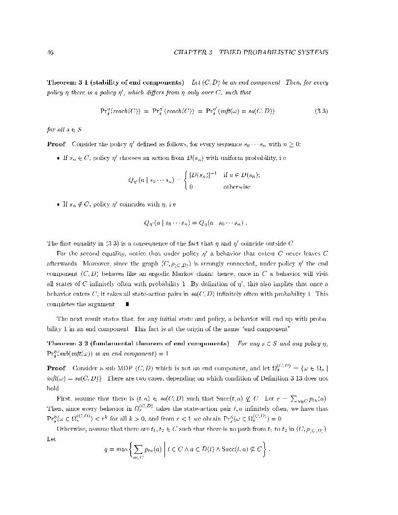
46 CHAPTER 3. TIMED PROBABILISTIC SYSTEMS
Theorem 3.1 (stability of end components) Let (C;D) be an end component. Then, for every
policy � there is a policy �0, which di�ers from � only over C, such that
Pr�s(reach(C)) = Pr�0
s (reach(C)) = Pr�0
s (inft(!) = sa(C;D)) (3.3)
for all s 2 S.
Proof. Consider the policy �0 de�ned as follows, for every sequence s0 � � � sn with n � 0:
� If sn 2 C, policy �0 chooses an action from D(sn) with uniform probability, i.e.
Q�0(a j s0 � � � sn) =
(jD(sn)j
�1 if a 2 D(sn);
0 otherwise.
� If sn 62 C, policy �0 coincides with �, i.e.
Q�0(a j s0 � � � sn) = Q�(a j s0 � � � sn) :
The �rst equality in (3.3) is a consequence of the fact that � and �0 coincide outside C.
For the second equality, notice that under policy �0 a behavior that enters C never leaves C
afterwards. Moreover, since the graph (C; �(C;D)) is strongly connected, under policy �0 the end
component (C;D) behaves like an ergodic Markov chain: hence, once in C a behavior will visit
all states of C in�nitely often with probability 1. By de�nition of �0, this also implies that once a
behavior enters C, it takes all state-action pairs in sa(C;D) in�nitely often with probability 1. This
completes the argument.
The next result states that, for any initial state and policy, a behavior will end up with proba-
bility 1 in an end component. This fact is at the origin of the name \end component".
Theorem 3.2 (fundamental theorem of end components) For any s 2 S and any policy �,
Pr�s(sub(inft(!)) is an end component) = 1.
Proof. Consider a sub-MDP (C;D) which is not an end component, and let (C;D)s = f! 2 s j
inft(!) = sa(C;D)g. There are two cases, depending on which condition of De�nition 3.13 does not
hold.
First, assume that there is (t; a) 2 sa(C;D) such that Succ(t; a) 6� C. Let r =Pu2C ptu(a).
Then, since every behavior in (C;D)s takes the state-action pair t; a in�nitely often, we have that
Pr�s(! 2 (C;D)s ) < rk for all k > 0, and from r < 1 we obtain Pr�s (! 2
(C;D)s ) = 0.
Otherwise, assume that there are t1; t2 2 C such that there is no path from t1 to t2 in (C; �(C;D)).
Let
q = max
�Xu2C
ptu(a)
���� t 2 C ^ a 2 D(t) ^ Succ(t; a) 6� C
�:

3.3. END COMPONENTS 47
s1
a a
c b
c
b
d a
b
a
cbs2 s3
s6s5s4
s7 s8
Figure 3.4: An MDP � = (S;A; p), with one of its end components depicted by dashed lines.
The lack of path from t1 to t2 in (C; �(C;D)) implies that, for every subsequence smamsm+1 � � � sn of
behavior in (C;D)s going from sm = t1 to sn = t2, there is j 2 [m::n� 1] such that Succ(sj ; aj) 62 C.
Thus, at most a fraction q of behaviors in (C;D)s can go from t1 to t2 without leaving (C;D). Since
every behavior ! 2 (C;D)s contains in�nitely many disjoint subsequences from t1 to t2, we have that
Pr�s(! 2 (C;D)s ) � qk for all k > 0. As q < 1, this implies again Pr�s (! 2
(C;D)s ) = 0.
The result then follows from the fact that there are only �nitely many sub-MDPs (C;D) in the
original MDP.
End components of Markov chains. As mentioned earlier, a Markov chain is an MDP in which
to each state is associated a single action. From an exam of the de�nition of end component, we
have the following characterization of end components of Markov chains.
Corollary 3.1 (end components of Markov chains) Consider an MDP � = (S;A; p) corre-
sponding to a Markov chain. A sub-MDP (C;D) is an end component i�:
� C is a closed recurrent class of the chain;
� D(s) = A(s) for all s 2 C.
The corollary is useful to adapt the model-checking algorithms we give for general MDPs to
Markov chains.

48 CHAPTER 3. TIMED PROBABILISTIC SYSTEMS
Example 3.5 (depicting end components) Figure 3.4 depicts an MDP � = (S;A; p) and a end
component (B;C) of the MDP. The states and actions of the MDP are de�ned by S = fs1; : : : ; s8g,
and A(s1) = fag, A(s2) = fa; bg, A(s3) = fa; cg, A(s4) = fcg, A(s5) = fb; cg, A(s6) = fbg,
A(s7) = fbg, A(s8) = fag.
The end component (B;C) of the MDP is given by B = fs2; s4; s5; s6; s7; s8g, and C(s2) = fag,
C(s4) = fcg, C(s5) = fcg, C(s6) = fbg, C(s7) = fbg, C(s8) = fdg.
3.3.2 Maximal End Components
Very often, we will be interested in the maximal end components contained in a given sub-MDP.
We introduce the following abbreviations to denote this set.
De�nition 3.14 (maxEC ) Given a sub-MDP (B;C), we denote by maxEC (B;C) the set of the
maximal end components of (B;C).
Moreover, given a subset of states B, we denote with AnS the restriction to domain B of the
action assignment A, and we abbreviatemaxEC (B;AnB) bymaxEC (B). In other words, maxEC (B)
is the set of maximal end components contained in the sub-MDP induced by the subset B of states.
Given a sub-MDP (C;D), the set of maximal end components of (C;D) can be computed using
the following algorithm, reminiscent of the procedure presented in [CY95, Proposition 4.2.3].
Algorithm 3.1 (computation of maximal end components)
Input: A sub-MDP (C;D).
Output: L = maxEC (C;D).
Initialization: L := f(C;D)g.
Repeat the following steps:
� Select (E;F ) 2 L.
� For all s 2 E, let F 0(s) := fa 2 F (s) j Succ(s; a) � Eg.
� Let E1; : : : ; En be the strongly connected components of the graph (E; �(E;F 0)), and let
Fi(s) = F 0(s) for all i 2 [1::n] and s 2 Ei.
� Replace (E;F ) 2 L with (E1; F1); : : : ; (En; Fn).
Until: L cannot be changed by the above iteration.
Given an MDP (S;A; p), it is easy to see that this algorithm runs in time polynomial inPs2S jA(s)j.

3.3. END COMPONENTS 49
3.3.3 State-Action Frequencies and End Components (z)
State-action frequencies represent the frequency with which state-action pairs appear in system
behaviors. They are a classical concept in the study of Markov decision processes, and they will
be used in the proofs of several results in the next chapters. Derman [Der70, Chapter 7] is an
introduction to the topic which also summarizes earlier work, such as Derman [Der63, Der64],
Derman and Strauch [DS66], and Strauch and Veinott [SV66]. Given a state-action pair s; a, let
Nksa be the random variable denoting the number of times a behavior has taken state-action pair
s; a before position k: formally,
Nksa =
k�1Xi=0
�[Xi = s ^ Yi = a] ; (3.4)
where �[true] = 1 and �[false] = 0. We de�ne the state-action frequency xsa(t; �) by
xsa(t; �) = limn!1
E�t fNnsag
n; (3.5)
provided that the limit exists: xsa(t; �) represents the long-run frequency with which the pair s; a
appears in a behavior, with initial state t and under policy �. When the initial state t and the policy
� are clear from the context, we write simply xsa.
Not surprisingly, there is a connection between state-action frequencies and end components, as
both of these are related to the long-run behavior of the system. One aspect of the connection is
described by the following theorem.
Theorem 3.3 (state-action frequencies and end components) Fix any initial state and any
policy �, and let
� = f(s; a) j xsa > 0g
be the set of state-action pairs having positive frequency, assuming that the limit (3.5) exists for all
state-action pairs. Then, � can be written as � =Sni=1 �i, where each sub(�i), for 1 � i � n, is an
end component.
Proof. De�ne the abbreviations
B� = fs 2 S j 9a : (s; a) 2 �g
E� =n(s; t) 2 S � S
��� 9a 2 A(s) : h(s; a) 2 � ^ t 2 Succ(s; a)io
:
The state-action frequencies are related by [Ber95]:
Xs;a2��
pst(a)xsa =Xa2A(t)
xta ; t 2 S : (3.6)

50 CHAPTER 3. TIMED PROBABILISTIC SYSTEMS
To show that � can be written in the form � =Sni=1 �i, with sub(�1); : : : ; sub(�n) end components,
we have to show that the two following statements hold.
� If (s; a) 2 �, then Succ(s; a) � B�. If (s; a) 2 � and t 2 Succ(s; a), then by (3.6) it must be
xtb > 0 for at least one b 2 A(t), which proves the result.
� The graph (B�; E�) is formed by the union of strongly connected subgraphs. By de�ning the
\ ow" fst as fst =Pa2A(s) xsapst(a), equations (3.6) can be rewritten as
Xs2S
fst =Xs02S
fts0 ; t 2 S ;
which can be interpreted as the law of ow conservation. If the graph (B�; E�) could not be
written as the union of strongly connected subgraphs, there would states s; t 2 B� such that
there is a path from s to t in (B�; E�), but no path from t to s, violating ow conservation.
An alternative proof of this result can be obtained by using the results of Derman [Der70,
Chapter 7]. There, Derman states that the limit points of the state-action frequencies are contained
in the convex hull determined by the state-action frequencies of deterministic policies. To obtain our
result, it su�ces to note that the sets of non-zero state-action frequencies of deterministic policies
correspond to the union of end components, as can be easily proved.
3.4 The Stochastic Shortest Path Problem
We now summarize some results about the stochastic shortest path (SSP) problem. This problem
will be a component of several model-checking algorithms for the probabilistic logics discussed in
this dissertation, so that it is convenient to introduce it at this early stage.
Informally, the stochastic shortest path problem consists in computing the minimum expected
cost for reaching a given subset of destination states, from any non-destination state of an MDP.
Bertsekas and Tsitsiklis [BT91] present a detailed account of this problem; this section is based on
[BT91] and [Ber95]. In Chapter 7, we will improve on these results by presenting solution methods
for instances of the SSP problem that cannot be solved with the methods of [BT91, Ber95].
Formally, an instance of the stochastic shortest path (SSP) problem is de�ned as follows.
De�nition 3.15 (instance of stochastic shortest path problem) An instance of the stochastic
shortest path problem consists of an MDP � = (S;A; p; U; c; g), in which the components U , c and
g are de�ned as follows:
� U is the set of destination states.

3.4. THE STOCHASTIC SHORTEST PATH PROBLEM 51
� c is the cost function, which associates to each state s 2 S � U and action a 2 A(s) the cost
c(s; a).
� g : U 7! IR is the terminal cost function, which associates to each s 2 U its terminal cost g(s).
De�ne TU = minfk j Xk 2 Ug, so that TU is a random variable indicating the position of �rst
entrance in U . Informally, the SSP problem consists in determining the minimum cost of reaching
U when following a policy that reaches U with probability 1. We call these policies SSP-proper.
De�nition 3.16 (SSP-proper policy) Given an instance (S;A; p; U; c; g) of SSP problem, a
policy � is SSP-proper if Pr�s(TU < 1) = 1 for all s 2 S � U . We denote by �P the class of
SSP-proper policies. A policy that is not SSP-proper is called SSP-improper.
The cost v�s of a policy � at s 2 S � U is de�ned by
v�s = E�s
�g(XTU ) +
TU�1Xk=0
c(Xk; Yk)
�: (3.7)
The SSP problem is formally de�ned as follows.
De�nition 3.17 (SSP problem) Given an instance (S;A; p; U; c; g) of SSP problem, determine
v�s = inf�2�
P
v�s
for all s 2 S � U .
Bertsekas and Tsitsiklis [BT91] provide solution methods for the SSP problem under the following
assumptions:
SSP Assumption 1: There is at least one Markovian SSP-proper policy.
SSP Assumption 2: If � is Markovian and not SSP-proper, then v�s =1 for at least one s 2 S�U .
As mentioned before, in Chapter 7 we will study the solution of SSP problems under di�erent
assumptions. The following theorem is taken from [BT91] (see also [Ber95]).
Theorem 3.4 (Bellman equations and SSP problem) Let (S;A; p; U; c; g) be an instance of
the SSP problem. Denote with v = [vs]s2S�U a vector of real numbers, and de�ne the functional L
on the space of v by
[Lv]s = mina2A(s)
�c(s; a) +
Xt2S�U
pst(a) vt +Xt2U
pst(a) g(t)
�s 2 S � U : (3.8)
If SSP Assumptions 1 and 2 are satis�ed, the following assertions hold:

52 CHAPTER 3. TIMED PROBABILISTIC SYSTEMS
� The functional L admits exactly one �xpoint v� such that v� = Lv�.
� The �xpoint v� of L is the single optimal solution of the following linear programming problem
on the set fvsgs2S�U of variables: MaximizeX
s2S�U
vs subject to
vs � c(s; a) +X
t2S�U
pst(a) vt +Xt2U
pst(a) g(t) s 2 S � U : (3.9)
� It is v�s = v�s for all s 2 S � U or, in vector form, v� = v�.
� Consider any Markovian policy � that selects at every s 2 S � U only actions that realize the
minimum on the right hand side of (3.8): formally,
Q�(a j s) > 0 i� a 2 arg mina2A(s)
�c(s; a) +
Xt2S�U
pst(a) vt +Xt2U
pst(a) g(t)
�;
for every s 2 S � U . Then, policy � is SSP-proper, and it is v�s = v�s = v�s for all s 2 S � U .
3.5 The Maximal Reachability Probability Problem
Another problem that will often recur in the model checking algorithms for the logics we present
is the maximal reachability probability problem. This problem consists in determining the maximal
probability with which a set of destination states can be reached from a given state. An algorithm
for solving this problem has been provided by Courcoubetis and Yannakakis [CY90]. We return
to the topic for the sake of completeness in our presentation of the veri�cation algorithms, and to
present the correctness proof for the algorithm, which is not included in [CY90]. Moreover, in the
next subsection we will present results that can be used to improve the e�ciency of the algorithms.
An instance of the maximal reachability probability problem is de�ned as follows.
De�nition 3.18 (instance of maximal reachability probability problem) An instance of
the maximal reachability probability problem consists of an MDP � = (S;A; p; U), where U � S is
the set of destination states.
The problem can be de�ned as follows.
De�nition 3.19 (maximal reachability probability problem) Given an instance � =
(S;A; p; U), the maximal reachability probability problem consists in computing the quantity
v�s = sup�Pr�s (reach(U))
for all s 2 S � U .

3.5. THE MAXIMAL REACHABILITY PROBABILITY PROBLEM 53
Sr
t1
1/2
1/2
2/3
1/3
2/5
3/5
0
1t2a
b
Se
U
Figure 3.5: A TPS with sets U , Sr and Se, along with the transition probabilities arising from theactions. The names of the actions, as well as the transition probabilities of deterministic actions,have not been indicated. The states of U and Se are labeled with the terminal cost function of thecorresponding SSP problem. The end component with state-action pairs (t1; a) and (t2; b) containedin Sr is indicated by dashed lines.
3.5.1 The Classical Algorithm
To solve the maximal reachability probability problem, we �rst compute the set of states from which
the maximal reachability probability is non-zero. Let Se � S be the set of states that cannot reach U ,
and let Sr = S� (Se [U). Thus, Sr is the subset of states not in U that can reach U . The following
lemma states that Sr [ U is exactly the set of states where the maximal reachability probability is
non-zero.
Lemma 3.1 The following assertions hold:
� sup� Pr�s(reach(U)) > 0 i� s 2 Sr [ U ;
� If s 2 U , then sup� Pr�s(reach(U)) = 1.
Proof. Immediate.
Thus, in the computation of the maximal reachability probability we can restrict our attention
to the set Sr. Unfortunately, the problem of computing the maximal reachability probability on all
states of Sr cannot be reduced to an instance of the SSP problem that satis�es SSP Assumptions 1
and 2. This is illustrated by the following example.
Example 3.6 Consider the TPS depicted in Figure 3.5. In the corresponding SSP problem, the
destination set is U [Se, and the terminal cost function is de�ned by g(s) = 1 if s 2 U , and g(s) = 0

54 CHAPTER 3. TIMED PROBABILISTIC SYSTEMS
if s 2 Se. The cost function c is always 0. In this way, for all s 2 Sr and all policies � it is
v�s = Pr�s (reach(U)).
Consider a deterministic policy �0 such that chooses action a at t1 and b at t2. Policy �0 is not
SSP-proper, since Pr�0t1 (reach(U [ Se)) = 0. On the other hand, the expected cost under �0 is such
that 0 � v�0s � 1 for all states s, since the cost c is always 0. This indicates that SSP Assumption 2
does not hold. In the next example, we will see that the �xpoint operator corresponding to the SSP
problem has more than one �xpoint, which would not be possible if SSP Assumption 2 held.
Consider a vector v = [vs]s2Sr , and de�ne on the space of v the functional
[Lv]s = maxa2A(s)
�Xt2Sr
pst(a) vt +Xt2U
pst(a)
�s 2 Sr : (3.10)
For any policy �, de�ne also v�s = Pr�s (reach(U)), and let v� = [v�s ]s2Sr . Unlike the case for the
instances of the SSP problem considered in the preceding section, the operator L may admit more
than one �xpoint. This is illustrated by the following example.
Example 3.7 Figure 3.6 depicts an MDP �0 together with two �xpoints of L; the lesser of
these two �xpoints is the least �xpoint. Note that the least �xpoint correspond to the reachability
probabilities: in the next theorems we show that this is no coincidence. We can trace the existence
of more than one �xpoint to the presence of end components in Sr.
Even though L admits more that one �xpoint, it can be proved that L admits a unique least
�xpoint, and that this least �xpoint corresponds to the solution to the maximal reachability prob-
ability problem. The proof is given later in the chapter. As a result, we will obtain the following
theorem.
Theorem 3.5 Consider the following linear programming problem, over the set fvsgs2Sr of vari-
ables: MinimizePs2Sr
vs subject to
vs �Xt2Sr
pst(a) vt +Xt2U
pst(a) s 2 Sr : (3.11)
This problem admits exactly one optimal solution vector v�. For every s 2 Sr, it is
sup� Pr�s (reach(U)) = v�s . Moreover, there is a Markovian (in fact, deterministic) policy �� such
that
Pr��
s (reach(U)) = sup�Pr�s (reach(U)) = max
�Pr�s(reach(U)) :
Note that the forms of the linear programming problems (3.9) and (3.11) are very similar, even
though the justi�cations for the reductions are di�erent.

3.5. THE MAXIMAL REACHABILITY PROBABILITY PROBLEM 55
S
U
e
U
Se
Sr
Sr
1/2
5/31/2
1/32/3
1/3
2/5
3/5
33
(0)
(1)
11/15
8/15
1/2
1/2
1/3 2/3
1/3
2/5
3/5
11/15 (1)
(0)
Figure 3.6: Two �xpoints of operator L on an MDP �0. The values 0 and 1 in U and Se are indicatedin parentheses, since they do not belong to the vector v. The end component in Sr is drawn withdashed lines. The �xpoint depicted below is the least �xpoint of L.

56 CHAPTER 3. TIMED PROBABILISTIC SYSTEMS
3.5.2 Improved Algorithms for Probabilistic Reachability (z)
In the preceding subsection, we have presented an algorithm that computes the maximal probability
of reaching a given subset of destination states U in the MDP. The method we have described is in
fact rather classical (see, for example, [CY90]). While the reduction to linear programming provides
us with the desired complexity bound for the algorithm, other computational approaches are also
possible. As the proof of Theorem 3.10 hints, methods based on value and policy iteration can
also be used. Such methods are described in several books on dynamic programming and optimal
control, among which Derman [Der70], Puterman [Put94], and Bertsekas [Ber95].
Since the computation of maximal reachability probabilities is a common problem in probabilistic
veri�cation, we present an improved algorithm that relies on two preprocessing step to reduce the
size of the linear programming problem to be solved. Since the preprocessing steps use only graph-
theoretical concepts, the reduction in the number of states can lead to overall time savings.
First Preprocessing Step
The �rst preprocessing step consists in adding to the set U all states U1 � Sr that can reach U with
maximal probability 1. This set U1 can be determined with the following algorithm, that will be
useful also in the future.
Algorithm 3.2 (set of states that can reach target with max probability 1)
Input: An MDP (S;A; p), and a subset U � S of states.
Output: The subset U1 � S � U of states that can reach U with maximal probability 1.
Method:
� Let S0 = S, A0 = A.
� Repeat:
{ Let B0 be the set of states that cannot reach S� in the graph (S0; �(S0;A0)).
{ Remove from S0 all states in B0.
{ Repeat:
� Remove from A0 all the actions leading to at least one removed state.
� Remove from S0 all states s 62 S� that have no actions left in A0.
{ Until no more states or actions can be removed from S0, A0.
� Until no more states or actions can be removed from S0, A0.
� Output U1 := S0.
The correctness of the algorithm is stated and proved as follows.

3.5. THE MAXIMAL REACHABILITY PROBABILITY PROBLEM 57
Theorem 3.6 If (S;A; p) and U are the inputs and U1 the output of the above algorithm, then
max�
Pr�s(reach(U)) = 1 i� s 2 U [ U1
for all s 2 S.
Proof. In one direction, we can prove by induction on the iteration on which a state s is removed
from U1 that max� Pr�s(reach(U)) < 1.
In the other direction, let �A be the value of A0 when the algorithm terminates. Notice that
�A(s) 6= ; for s 2 U1, or else s would have been eliminated during the iteration of the algorithm.
Consider the policy �1 that chooses at each state s 2 U1 an action from �A(s) with uniform probability.
Notice that every state of U1 can reach U in (U1 [U; �(U1[U; �A)): otherwise, the state would have
been removed from U1 by the algorithm. Thus, in the Markov chain arising from �1 there is no
closed recurrent class that is contained in U1. Under �1, a behavior will therefore leave U1 with
probability 1. Note also that the only way a behavior can leave U1 under policy �1 is by passing
through U . Hence, we conclude that under �1 a behavior from any state s 2 U1 will reach U with
probability 1. This yields the result.
Once the correctness of the algorithm has been established, the �rst preprocessing step can be
stated and proved correct as follows.
Theorem 3.7 (�rst preprocessing step) Let (S;A; p; U) be an instance of maximal reachability
probability problem, and let U1 be the set computed by Algorithm 3.2 on input (S;A; p) and U . Then,
for all s 2 S � U it is
max�
Pr�s(reach(U)) = max�
Pr�s(reach(U [ U1)) : (3.12)
Thus, we can substitute the instance (S;A; p; U) with an equivalent instance (S;A; p; U[U1) in which
the maximal reachability probability must be computed for a smaller set of states.
Proof. Let B be the set of states that cannot reach U . Notice that these states also cannot reach U1,
so that they trivially satisfy (3.12). Also, by the correctness of Algorithm 3.2 it is Pr�s (reach(U)) = 1
for all s 2 U1, so that the states in U1 also satisfy (3.12).
For a state s 2 S � (U [ U1 [ B), the inequality
max�
Pr�s (reach(U)) � max�
Pr�s(reach(U [ U1))
trivially holds. To show that in fact equality holds, let �0 be a Markovian policy that realizes the
maximum for the left hand side of (3.12). From �0, we can de�ne a modi�ed policy �m, which
outside of U1 behaves like �0, and inside of U1 coincides with the policy �1 de�ned in the proof of

58 CHAPTER 3. TIMED PROBABILISTIC SYSTEMS
the previous theorem. It is easy to check that under �m it is
max�
Pr�s(reach(U [ U1)) = Pr�ms (reach(U)) = Pr�0s (reach(U [ U1)) ;
which concludes the proof.
Second Preprocessing Step
The second preprocessing step consists in \short-circuiting" the end components in Sr, replacing
them by single states, while preserving the reachability probabilities. This is done by applying the
following algorithm.
Algorithm 3.3 (end component elimination)
Input: Instance � = (S;A; p; U), together with subsets Sr and Se.
Output: Instance b� = (bS; bA; bp; bU), with the subsets bSe, bSr of states.Method: Let f(B1; D1); : : : ; (Bn; Dn)g = maxEC (Sr). De�ne bU = U , bSe = Se, and
bS = S [ fbs1; : : : ; bsng � n[i=1
Bi bSr = Sr [ fbs1; : : : ; bsng � n[i=1
Bi :
The action sets are de�ned by:
s 2 S �
n[i=1
Bi : bA(s) = fhs; ai j a 2 A(s)g
1 � i � n : bA(bsi) = nhs; ai ��� s 2 Bi ^ a 2 A(s)�D(s)o:
For s 2 bS, t 2 S �Sni=1 Bi and hu; ai 2 bA(s), the transition probabilities are de�ned by
bpst(hu; ai) = put(a) bpsbsi(hu; ai) = X
t2Bi
put(a) :
The following theorem enables to use b� for the computation of the maximal reachability proba-
bilities in �.
Theorem 3.8 Let b� be the MDP obtained from � as in Algorithm 3.3. Denoting with Pr, cPr theprobabilities computed in �, b�, it is
s 2 Sr �
n[i=1
Bi : max�
Pr�s(reach(U)) = max�
cPr�s (reach(bU)) (3.13)

3.5. THE MAXIMAL REACHABILITY PROBABILITY PROBLEM 59
s 2 Bi; 1 � i � n : max�
Pr�s(reach(U)) = max�
cPr�si(reach(bU)) : (3.14)
The proof of this theorem is presented later in the section. The following example illustrates the
application of Algorithm 3.3.
Example 3.8 Figure 3.7 depicts an MDP �, and the MDP b� obtained by applying Algorithm 3.3
to �. The actions corresponding to the end components of Sr are drawn using dashed lines. These
end components are
subf(s3; d); (s4; i); (s7; j)g subf(s5; f); (s6; g)g
and they are replaced by the new states bs1 and bs2. This example illustrates the potential reductionof the state-space of the system e�ected by the algorithm.
3.5.3 Proof of the Results (z)
We now prove the results on the maximal reachability probability problem. To simplify the ar-
guments, we assume that once the set U of destination states is entered, it can never be exited.
Formally, this is expressed by the requirement Succ(s; a) � U for all s 2 U and a 2 A(s). It is
immediate to see that this assumption does not a�ect the generality of the arguments.
The Standard Algorithm
First, we present a preparatory lemma.
Lemma 3.2 If v� = Lv�, then v�s � 0 for all s 2 Sr.
Proof. Assume that v� = minfv�t j t 2 Srg < 0, and let S� = fs 2 Sr j v�s = v�g be the subset
of Sr consisting of the states at which v� reaches its minimum value v�. Since each state of Sr can
reach U , there must be s 2 S� and a 2 A(s) such that Succ(s; a) 6� S�. This implies that
v�s <Xt2Sr
pst(a) v�t +
Xt2U
pst(a) ;
contradicting the fact that v� is a �xpoint of L.
Our second result states that the �xpoints of L provide an upper bound for v�.
Theorem 3.9 If v� = Lv�, then v�s � v�s for every �.
Proof. From (3.10), it is
v�s �Xt2Sr
pst(a) v�t +
Xt2U
pst(a)

60 CHAPTER 3. TIMED PROBABILISTIC SYSTEMS
s8
s9
Se
s s
Π
s9
s8
Se
a
cb
e f
ghj
s s
s
3
s s2
s6
7
5
1
s4
1/3
1/31/3
d
i
Π
l
mU
e f
s1 s2
b
h
c
a
1 2
1/32/3
Um
l
k
k
Figure 3.7: An example of application of Algorithm 3.3. To simplify the diagrams, we have indicatedonly the transition probability corresponding to action c. The new states introduced to replace thezero-cost end components are indicated by �lled circles.

3.5. THE MAXIMAL REACHABILITY PROBABILITY PROBLEM 61
for all s 2 Sr and a 2 A(s). Iterating, for a general policy � and n � 0 we have
v�s �Xt2Sr
Pr�s(Xn = t) v�t + Pr�s (Xn 2 U)
for all n � 0. Taking the limit n!1 and using Lemma 3.2, we obtain
Pr�s(reach(U)) = limn!1
Pr�s (Xn 2 U) � v�s � limn!1
Xt2Sr
Pr�s (Xn = t) v�t � v�s ;
which concludes the proof.
Given a deterministic policy � we indicate by �(s) 2 A(s) the action chosen by � at s 2 S. We
also say that a Markovian policy � is proper if
Pr�s (reach(S � Sr)) = 1
for every s 2 Sr. To prove our main result, we need the following additional lemma.
Lemma 3.3 Given a proper deterministic policy �, there is a function � : Sr 7! Sr [ U with the
following properties:
1. �(s) 2 argmaxnv�t
��� t 2 Succ(s; �(s))o, for all s 2 Sr.
2. v�s � v��(s)
, for all s 2 Sr.
3. The graph (Sr [U;E) with edges E = f(s; �(s)) j s 2 Srg is an in-forest (i.e. a forest in which
edges are directed towards the roots) with roots in U .
Proof. Extend v� to U by v�s = 1 for s 2 U . We construct � as follows. Initially, � is unde�ned
on all s 2 Sr; we then iterate the following steps:
� Choose s 2 Sr such that � is not yet de�ned on s, and such that there is
t 2 argmaxnv�t
��� t 2 Succ(s; �(s))o
such that either t 2 U or �(t) is already de�ned.
� De�ne �(s) = t.
The iteration continues until the domain of � cannot be further extended.
If the iteration de�nes � on all Sr, it is immediate to see that properties 1, 2 and 3 hold. To see
that the iteration de�nes � on all Sr, assume towards the contradiction that after a certain number

62 CHAPTER 3. TIMED PROBABILISTIC SYSTEMS
of iterations � has been de�ned on a subset Sd � Sr of states, and no s 2 Sr � Sd can be found for
the next iteration. Let
Sm = arg maxs2Sr�Sd
v�s
be the subset of Sr � Sd where v� attains maximal value. Since � is proper, there must be s0 2 Sm
such that
Succ(s0; �(s0)) 6� Sm : (3.15)
Since the iteration cannot extend the domain of �, it is also
v�t < v�s0 (3.16)
for all t 2 (U[Sd)\Succ(s0; �(s0)). Putting together (3.15) and (3.16), and considering the de�nition
of Sm again, we get
v�s0 =X
t2Sr[U
pst(�(s0)) v�t < v�s0 ;
which is the desired contradiction.
Finally, we show that L has at least one �xpoint, and that the �xpoint corresponds to a reacha-
bility probability attained by a policy.
Theorem 3.10 There is a deterministic policy � such that v� = Lv�.
Proof. Notice that there is at least one proper policy �0, which can in fact be determined when
the set of states Sr that can reach U is computed. Starting from �0, we construct a sequence of
proper deterministic policies �0; �1; : : :. The construction proceeds as follows.
First, given a proper deterministic policy �k, for k � 0, we construct a function �k : Sr 7! S
with the properties mentioned in the previous lemma. Next, we let
Sk =
�s
���� v�ks < maxa2A(s)
�Xt2Sr
pst(�k(s)) v�kt +
Xt2U
pst(�k(s))
��: (3.17)
If Sk = ;, the sequence of policies terminates with �k. Otherwise, we choose sk2 Sk, and we de�ne
policy �k+1 to be the policy that coincides with �k everywhere except at sk, where
�k+1(sk) = arg max
a2A(s)
�Xt2Sr
pst(�k(s)) v�kt +
Xt2U
pst(�k(s))
�:
If there is more than one action realizing the maximum, one such action is chosen arbitrarily. To
see that �k+1 is also proper, let �0k be the function that coincides with �k on Sr �fs
kg, and de�ned
on sk by
�0k(sk) = argmax
nv�kt
��� t 2 Succ(sk; �k+1(sk))o:

3.5. THE MAXIMAL REACHABILITY PROBABILITY PROBLEM 63
If there is more than one state realizing the maximum, one such state is chosen arbitrarily. Like �k,
also �0k induces a in-forest of states with roots in U . In fact, no loops in �0k can be created, due
to Property 2 of �k, to the strict inequality in (3.17), and to the de�nition of �0k in terms of �k.
This indicates that �k+1 is also proper, since every state of Sr can reach U with positive probability
under �k+1.
Since �k+1 is proper, v�k+1 is well-de�ned, and by the monotonicity of L and (3.17) we have
v�k < v
�k+1 . As there is only a �nite number of deterministic policies, a value of k = K will be
reached for which there is no state s 2 Sr that satis�es (3.17). If �K is the �nal policy, the absence
of s satisfying (3.17) shows that v�K = Lv�K ; the conclusion follows then from the fact that �K is
proper.
Putting together this theorem and the previous one, we have the following corollary, which
connects the �xpoints of L to the desired maximum reachability probability.
Corollary 3.2 For every state s 2 Sr, it is
sup�Pr�s (reach(U)) = v�s ;
where v� is the least �xpoint of L. Moreover, there is a deterministic policy � such that v� = v�, so
that the supremum is attained by at least one policy.
Proof. By Theorem 3.10, L admits a �xpoint v� = v�� for some deterministic ��. By Theorem 3.9,
v�� � v
� for all �. This yields the result.
To complete the proof of Theorem 3.5, we need to prove that the linear programming problem
(3.11) admits v� as unique optimal solution, where v� is the least �xpoint of L. The argument is
completely standard (see for example Bertsekas [Ber95]); we sketch it here purely for the sake of
completeness, since we will often use similar arguments in this dissertation.
Proof of Theorem 3.5. Let v� be the least �xpoint of L. Clearly, v� is a feasible solution of the
linear programming problem.
In the other direction, consider a feasible solution v� of the linear programming problem. From
(3.11), reasoning as in the proof of Theorem 3.9 we can show that v� � v� for all policies �. By
Theorem 3.10, this implies v� � v�.
These two considerations show that v� is the least feasible solution of the linear programming
problem.
The Improved Algorithm
Before proving Theorem 3.8, we need a preparatory lemma. To state the lemma, we introduce the
following notation. Given a Markovian policy �, we denote by S(�) the following system of equations

64 CHAPTER 3. TIMED PROBABILISTIC SYSTEMS
in fvsgs2Sr :
vs =X
a2A(s)
Xt2Sr
pst(a)Q�(a j s) vt +X
a2A(s)
Xt2U
pst(a)Q�(a j s) s 2 Sr :
Lemma 3.4 If a Markovian policy � is proper, then the system of equations S(�) has v� as unique
solution.
Proof. Let P = [pst]s;t2Sr be the matrix of the Markov chain associated to � on Sr, and de�ne
q = [qs]s2Sr by
qs =X
a2A(s)
Xt2U
pst(a)Q�(a j s)
for all s 2 Sr. Then, S(�) can be rewritten as v = Pv + q. Since � is proper, P is the matrix of a
transient Markov chain, and det(I �P ) 6= 0. Thus, S(�) admits a unique solution. The lemma then
follows from the fact that the reachability probabilities v� also satisfy S(�).
Theorem 3.8 can be proved as follows.
Proof of Theorem 3.8. To prove the result, we break up the transformation e�ected by Algo-
rithm 3.3 in two steps. Let f(B1; D1); : : : ; (Bn; Dn)g = maxEC (Sr). First, from � we construct an
MDP e� = (S; eA; ep) de�ned as follows:
eA(s) =(fhs; ai j a 2 A(s)g if s 62
Sni=1 Bi;
fht; ai j t 2 Bi ^ a 2 A(t)�Di(t)g if s 2 Bi, 1 � i � n.(3.18)
and epsu(ht; ai) = ptu(a) for all s; u 2 S and ht; ai 2 eA(s). The sets U and Sr, like S, are not changed.
Let eL be the operator de�ned for e� in the same way as L for �. We have the following fact.
Fact 1. If v� = eLv� is a �xpoint of eL, and s; t 2 Bi, for 1 � i � n, then v�s = v�t .
To see this, note that for 1 � i � n all states in Bi have the same set of actions, which lead to the
same sets of destinations: from the de�nition of eL, we see that the value of v at all states of Bi must
be the same. This leads to our next fact.
Fact 2. If v = eLv, then v = Lv.
This can be seen as follows. Assume v = eLv. On S �Sni=1 Bi, L and eL are the same. Consider
thus s 2 Bi, 1 � i � n. If a 2 A(s) then hs; ai 2 eA(s), and from
vs �Xt2S
epst(hs; ai) vt

3.5. THE MAXIMAL REACHABILITY PROBABILITY PROBLEM 65
we have
vs �Xt2S
pst(a) vt : (3.19)
Moreover, for each state s 2 Bi there is at least one action a 2 Di(s). From Succ(s; a) � Bi follows
vs =Xt2S
pst(a) vt ; (3.20)
showing that the maximum in the de�nition of L is realized at least for one state-action pair. From
(3.19) and (3.20) follows then v = Lv, concluding the proof of Fact 2.
Consider a reduction to the SSP problem in which we take the destination set to be S � Sr, the
cost function c to be 0 for all state-action pairs, and the terminal cost g(s) equal to �1 for s 2 U
and 0 for s 2 S � (Sr [ U). Since there are no end components in Sr, it is fPr�s(reach(S � Sr)) = 1
for all �, so that all policies are SSP-proper. Thus, from Theorem 3.4 we have the following fact.
Fact 3. There is exactly one v� such that v� = eLv�.From the �xpoint v� we construct a deterministic policy e� as follows. For each s 2 Sr, de�ne
the set Amax(s) by
Amax(s) = argmaxa2eA
�Xt2Sr
epst(a) v�t +Xt2U
epst(a)�: (3.21)
At each s 2 Sr, policy e� chooses deterministically an arbitrary action selected from Amax(s). From
Fact 1, for each 1 � i � n it is Amax(s) = Amax(t) for all s; t 2 Bi. Thus, we can force e� to choosethe same action hui; aii at all states of Bi, for 1 � i � n.
Since there are no end components in Sr, policy e� is proper. Since e� chooses only actions that
realize the maximum in (3.21), by Theorem 3.4 we have v� = ve� .
From e�, we construct a Markovian policy � for � such that v� = ve� . At s 2 S �Sni=1Bi, policy
� behaves like e�. At s 2 Bi, with 1 � i � n, there are two cases:
� if s = ui, policy � chooses deterministically ai;
� if s 6= ui, policy � chooses with uniform probability an action from the set Di(s).
The idea behind this de�nition of � is as follows. Under �, when a behavior enters Bi it starts a
random walk. If uninterrupted, this random walk would lead the behavior to visit each state of
Bi with probability 1. The random walk terminates when the behavior visits ui, at which point �
chooses ai, imitating the choice of hui; aii e�ected by e�. From this explanation, we see that � is
proper.
Since � is proper, by the previous lemma the system of equations S(�) has v� as unique solution.
To show that v� = ve� , we show that ve� is also a solution of S(�). The proof is by cases:

66 CHAPTER 3. TIMED PROBABILISTIC SYSTEMS
� If s 2 Bi for 1 � i � n, and s 6= ti (where hti; aii is the action chosen by e� ), then policy �
chooses with uniform probability an action from Di(s). These actions lead only to destinations
in Bi. From Fact 1, ve� = v� is constant on Bi, and the result follows.
� If s 2 Bi and s = ti, for 1 � i � n, or if s 2 Sr �Sni=1 Bi, the systems of equations S(�) and
S(e�) coincide on s, and the result follows.
Since ve� = v�, it is also v� = v
�, and from Fact 2 it is v� = v� = Lv�. By Theorem 3.9, policy �
realizes the maximal probability of reaching U , indicating that this maximal probability is equal to
v�.
To complete the proof, we note that MDP b� is obtained from e� by merging the states belonging
to each Bi, for 1 � i � n. The justi�cation for this merging step is as follows.
By construction, if s; t 2 Bi for some 1 � i � n, then eA(s) = eA(t), and for any other state u 2 S
and a 2 eA(s) we have epsu(a) = eptu(a). This indicates that s; t are in fact identical copies. The
MDP b� is obtained from e� by merging all the identical copies corresponding to Bi into a single
representative state bsi, letting bpu;si(a) = Xs2Bi
epus(a)for every a 2 bA(s).
From these considerations, we see that the merging step does not in uence the solution of the
�xpoint equations. Speci�cally, if v� = bLv� is a �xpoint for b�, then we can show that
s 2 Sr �
n[i=1
Bi : v�s = v�s
s 2 Bi; 1 � i � n : v�si = v�s ;
justifying relations (3.13) and (3.14).

Chapter 4
Basic Probabilistic Logic
Several types of formalisms have been applied to the formal speci�cation of probabilistic properties
of systems, as we discussed in the introduction. In this dissertation, we follow the approach of
extending branching-time temporal logics with probabilistic operators. The reason branching-time
temporal logics are preferred to linear-time ones as the basis of probabilistic extensions is that
probability measures on system behaviors are structurally similar to path quanti�ers, as we will see.
Our probabilistic extensions are based on the branching-time temporal logics CTL and CTL*,
introduced in Emerson and Sistla [CE81], Ben-Ari, Pnueli, and Manna [BAPM83] and Emerson
and Halpern [EH85]. The extensions are obtained by augmenting CTL and CTL* with operators
that enable the expression of probabilistic system properties. As mentioned in the introduction,
we consider four new operators: P, D, �P, and �D, which enable the expression of four types of
probabilistic properties, as summarized in Table 1.1.
In this chapter we consider the operators P and D, postponing to the next chapter the introduc-
tion of �P and �D and a detailed discussion of the classi�cation of probabilistic temporal operators.
The operator P is used to express bounds on the probability of system behaviors. Precisely, if � is
a formula encoding a property of behaviors, the formula P�a� (resp. P�a�) holds at a state if the
probability of satisfying � from s is at least (resp. at most) a, under any policy. The operator D is
used to express bounds on average times. If is a state property, formula D�a (resp. D�a ) holds
at a state s if a state that satis�es can be reached from s in average time at least (resp. at most)
a, regardless of the policy.
4.1 A Brief History of Probabilistic Temporal Logics
The practice of extending branching-time logics with additional operators for the expression of
probabilistic properties is not new. The �rst probabilistic extension of branching-time logics for the
expression of probabilistic system properties was proposed by Hansson and Jonsson [HJ89, HJ94].
67

68 CHAPTER 4. BASIC PROBABILISTIC LOGIC
This proposal considered systems modeled as Markov chains and introduced a temporal logic, PCTL,
to specify the probability of satisfying temporal formulas within a given amount of chain transitions.
The formulas of PCTL are obtained by adding subscripts and superscripts to CTL formulas; as an
example, the formula 3<50�0:8� means that with probability 0:8, formula � will become true after a
sequence of less than 50 state transitions of the Markov chain.
The model-checking algorithms of [HJ89, HJ94] rely on results on Markov chains and dynamic
programming. Their time complexity is polynomial in the size of the system and linear in the
numerical values of the time bounds appearing in the superscripts. This time complexity is typical
of the algorithms that rely on the direct or indirect use of clocks, such as the dynamic programming
recursions used to compute the probability of meeting timing deadlines.
The logic PCTL was later extended by Hansson [Han94] to systems that include nondeterminism,
and which provide a more re�ned model of time. The model-checking algorithms proposed by [Han94]
for this extension are based on the enumeration of all possible deterministic policies, leading to
exponential time-complexity in the size of the system.
Aziz et al. [ASB+95] introduced the logic pCTL*, derived from CTL* by adding the operator P,
which is de�ned as in the logics presented here. Two types of system models are considered: Markov
chains and generalized Markov chains (called Markov processes and generalized Markov processes in
[ASB+95]). The model checking of pCTL* speci�cations on Markov chains is based on the results
of Courcoubetis and Yannakakis [CY88], and is of polynomial complexity in the size of the Markov
chain. Generalized Markov chains are Markov chains in which some transition probabilities are given
as parameters; these parameters must satisfy a speci�ed set of constraints. The model checking of
pCTL* speci�cations on generalized Markov chains is shown to be elementarly decidable using results
from the theory of the real closed �eld, but no practical veri�cation algorithm is provided.
The logic pCTL* was later extended to systems with nondeterminism by Bianco and de Alfaro
[BdA95], who also provided model-checking algorithms for the resulting logics. Later, [dA97] con-
sidered a computational model related to TPSs, and introduced the operator D for the expression
of average times. The model-checking algorithms presented improve on [BdA95], and are essentially
the ones presented for pTL and pTL* in this chapter.
Recent developments include the study of probabilistic model checking in presence of fairness
by Baier and Kwiatkowska [KB96]. This work, which was in uential in the development of our
approach to fairness, will be discussed in detail in Chapter 8.
An algorithm for the symbolic model-checking of pCTL and pCTL* formulas on Markov chains
was presented by Baier, Kwiatkowska and Ryan [BKR+97]. The algorithm proposed is a symbolic
implementation of the algorithms described in [BdA95, dA97] for the case of Markov chains. The
algorithm usesMulti-Terminal Binary Decision Diagrams [CFZ96] to represent transition probability
matrices and to compute the necessary reachability probabilities; this representation is found to be
more compact and e�cient than one based on traditional sparse matrices. It would be of great

4.2. THE LOGICS PTL AND PTL* 69
interest to study how this symbolic approach can be applied to systems with nondeterminism, and
to the model-checking algorithms presented in this dissertation for the various logics presented.
The operators D, �P and �D have been introduced in the work that led to this dissertation, along
with the classi�cation of probabilistic properties given in Table 1.1.
4.2 The Logics pTL and pTL*
The de�nitions of syntax and semantics of the logics pTL and pTL* are taken from [dA97], except
that the use of instrumentation clocks has been replaced by the notion of expected transition times
in TPSs.
4.2.1 Syntax of pTL and pTL*
As in CTL and CTL*, the formulas of pTL and pTL* are divided in two mutually exclusive classes:
the class Stat of state formulas (whose truth value is evaluated on the states), and the class Seq of
sequence formulas (whose truth value is evaluated on in�nite sequences of states). To de�ne these
classes, we assume that we have a �xed set V of typed variables, and �xed sets of interpreted predicate
and function symbols. We let Atomic be the class of atomic formulas containing all �rst-order logic
formulas formed from variables in V using these interpreted predicate and function symbols. The
classes Stat and Seq are then de�ned by the following inductive clauses.
State formulas:
� 2 Atomic =) � 2 Stat (4.1)
� 2 Stat =) :� 2 Stat (4.2)
�; 2 Stat =) � ^ 2 Stat (4.3)
� 2 Seq =) A�; E� 2 Stat (4.4)
� 2 Seq =) P./a� 2 Stat (4.5)
� 2 Stat =) D./b� 2 Stat (4.6)
Sequence formulas:
� 2 Stat =) � 2 Seq (4.7)
� 2 Seq =) :� 2 Seq (4.8)
�; 2 Seq =) � ^ 2 Seq (4.9)

70 CHAPTER 4. BASIC PROBABILISTIC LOGIC
� 2 Seq =) 2�; 3� 2 Seq (4.10)
�; 2 Seq =) � U 2 Seq : (4.11)
In the above de�nition, ./ stands for one of f<;�;�; >g, and a and b are real numbers such that
0 � a � 1 and b � 0. The temporal operators 2, 3, U , and the path quanti�ers A, E are taken
from CTL*. As usual, the other propositional connectives are de�ned in terms of :, ^.
Just as CTL is a restricted version of CTL*, the logic pTL is a restricted version of pTL*; its
de�nition is obtained by replacing clauses (4.7){(4.11) with the clauses
� 2 Stat =) 2�; 3� 2 Seq (4.12)
�; 2 Stat =) � U 2 Seq : (4.13)
4.2.2 Semantics
Consider a TPS � = (S;A; p; Sin; time; I). The semantics of pTL and pTL* formulas with respect
to � is de�ned by two satisfaction relations, one for state formulas and one for sequence formulas.
For � 2 Stat, we indicate with s j= � the satisfaction of � at s 2 S. For 2 Seq and k 2 IN we
indicate with ! j=k the satisfaction of at position k of behavior ! 2Ss2S s. The base case for
(4.1) and the cases for the logical connectives are immediate.
Temporal Operators
The satisfaction relation ! j=k � for a behavior ! and � 2 Seq is de�ned in the usual way (see for
example [MP93, MP91]):
� 2 Stat ! j=k � i� sk j= �
� 2 Seq ! j=k 2� i� 8i : [i � k ! ! j=i �]
� 2 Seq ! j=k 3� i� 9i : [i � k ^ ! j=i �]
�; 2 Seq ! j=k � U i� 9i :hi � k ^ ! j=i ^ 8j : (k � j < i! ! j=j �)
i:
Path Quanti�ers
The semantics of the path quanti�ers is de�ned as in CTL and CTL* [Eme90]. For s 2 S and
� 2 Seq, it is
s j= A� i� 8! 2 s : ! j=0 �
s j= E� i� 9! 2 s : ! j=0 � :

4.2. THE LOGICS PTL AND PTL* 71
Probabilistic Operator P
The semantics of the probabilistic quanti�ers is de�ned as in [BdA95]: for sequence formula � 2 Seq,
state s 2 S, probability bound 0 � a � 1 and ./2 f<;�;�; >g,
s j= P./a� i� 8� : Pr�s (! j=0 �) ./ a : (4.14)
The intuitive meaning of (4.14) is that P./a� holds at s 2 S if a behavior from s satis�es � with
probability ./ a, regardless of the policy.
Average-Time Operator D
Given a behavior ! and a state formula � 2 Stat, let T� = minfk j ! j=k �g be the �rst position of
! at which � holds, with T� = 1 if 8k : ! 6j=k �. For state s 2 S, formula � 2 Stat, bound b � 0
and ./2 f<;�;�; >g we de�ne
s j= D./b� i� 8� : E�s
�T��1Xk=0
time(Xk; Yk)
�./ b : (4.15)
The intuitive meaning of (4.15) is that D./d� holds at s 2 S if the TPS reaches a �-state in average
time ./ d, regardless of the policy.
To see that the semantics of pTL and pTL* is well de�ned, it is possible to show by induction
on the structure of formulas that the events and functions mentioned in the above de�nitions are
measurable. In particular, if � 2 Seq and s 2 S, the truth-set f! 2 s j ! j=0 �g is measurable; if
� 2 Stat, then T� is a random time, andPT��1k=0 time(Xk; Yk) is a measurable function.
We say that a TPS satis�es a speci�cation if the speci�cation holds on all initial states of the
TPS.
De�nition 4.1 (validity over TPS) Given a TPS � = (S;A; p; Sin; time; I) and a pTL or pTL*
speci�cation � 2 Stat, we say that � satis�es �, written � j= �, i� s j= � for all s 2 Sin.
4.2.3 Examples of Speci�cation
We present here only two simple examples of speci�cations that can be written in the logics pTL
and pTL*. In spite of their simplicity, these examples illustrate some typical uses of the operators
P and D.
Example 4.1 (expected time to failure) Assume that � is a TPS that models an industrial
plant. Assume that we have the following atomic state formulas:
� a formula good which characterizes system states lying inside a prescribed safe control region;

72 CHAPTER 4. BASIC PROBABILISTIC LOGIC
� a formula broken which characterizes system states at which some failure has occurred.
The states satisfying :good ^ :broken are states that do not lie in the safe control region, but at
which no failure has yet occurred. The pTL formula
A2�good! D�abroken
�
speci�es that, if the system state is in the safe control region, a failure will occur with expected time
no less than a.
Example 4.2 (probability of deadlock) Assume that � is a TPS that models a distributed
system. Assume that we have the following atomic state formulas:
� formulas task-start, task-in-prog, task-complete which characterize the states at which a task
is begun, is in progress, and has been completed, respectively;
� a formula deadlock which characterizes states at which a deadlock has occurred.
We assume that the above four formulas are mutually exclusive. The pTL* formula
A2htask-start! P�a
�(task-start _ task-in-prog) U task-comp
�i
speci�es that, whenever a new task is started, the probability it completes without deadlocks is at
least a.
4.3 Checking Non-Zenoness
The �rst task in the veri�cation of a TPS is to check whether it is non-Zeno. The following theorem
provides a criterion for non-Zenoness that leads to an e�cient checking algorithm.
Theorem 4.1 (criterion for non-Zenoness) Let � = (S;A; p; Sin; time; I) be a TPS. For each
s 2 S, de�ne B(s) = fa 2 A(s) j time(s; a) = 0g to be the set of actions with zero expected time
from s. Then, � is Zeno i� there is an end component (C;D) of (S;B) which is reachable in the
graph (S; �S) from some initial state in Sin.
Proof. In one direction, assume that there is an end component (C;D) of (S;B) reachable from
a state s0 2 Sin in the graph (S; �S). Since C is reachable from s0, there is a policy � such that
Pr�s0(9k : Xk 2 C) > 0. By Theorem 3.1, there is a policy �0 such that Pr�s0(I(!) = (C;D)) > 0.
Since (C;D) is contained in (S;B), this leads to
Pr�0
s0
� 1Xi=0
time(Xi; Yi) <1
�> 0 ;

4.4. MODEL CHECKING FOR OPERATOR P IN PTL* 73
showing that � is Zeno.
Conversely, assume that (S;B) does not contain any end component. By Theorem 3.2, the set
inft(!) is an end component with probability 1. Since for each end component (C;D) reachable
from an initial state there is at least one state-action pair (s; a) 2 sa(C;D) with time(s; a) > 0, with
probability 1 every behavior takes in�nitely many steps with time > 0. This leads immediately to
Pr�s
� 1Xi=0
time(Xi; Yi) =1
�= 1
for all � and all s 2 Sin, which is the de�nition of non-Zenoness.
This theorem leads immediately to the following algorithm.
Algorithm 4.1 (checking non-Zenoness)
Input: TPS � = (S;A; p; Sin; time; I).
Output: Yes/no answer, stating whether � is non-Zeno.
Method: For each s 2 S let B(s) = fa 2 A(s) j time(s; a) = 0g, and use Algorithm 3.1 to compute
the set maxEC (S;B) = f(C1; D1); : : : ; (Cn; Dn)g of maximal end components of (S;B). Check
whetherSni=1 Ci is reachable from Sin, and answer \no" if it is, and \yes" if it is not.
4.4 Model Checking for Operator P in pTL*
In this and in the next section we present algorithms to decide whether a TPS � satis�es a speci-
�cation � written in pTL or pTL*. The model checking algorithms share the same basic structure
of those proposed in Emerson and Lei [EL85] for CTL and CTL*. Given a TPS � and a formula
� 2 Stat, the algorithms recursively evaluate the truth values of the state subformulas of � at all
states s 2 S, following the recursive de�nitions (4.1){(4.6), until the truth value of � itself can be
computed at all s 2 S. Since the logics pTL and pTL* are obtained by adding the operators P and
D to CTL and CTL*, we need to examine only the cases corresponding to these operators. In this
section, we present algorithms for the model checking of the P operator; in the next section we will
present the algorithms for D.
The model checking of operator P in the logic pTL* can be done using the results of Courcoubetis
and Yannakakis [CY90]; we will present below an alternative algorithm. The model checking of
operator P in the logic pTL can be done using the algorithms for pTL*, since pTL is a subset of
pTL*. However, for the case of pTL it is also possible to use a simpler algorithm, due to Bianco
and de Alfaro [BdA95]; we will present this algorithm in Section 4.8. The algorithms for the model
checking of operator D are the same in pTL and pTL*.

74 CHAPTER 4. BASIC PROBABILISTIC LOGIC
From de�nition (4.14), to decide whether s j= P./a� for a state s and a formula � 2 Seq it su�ces
to compute the minimum and maximum probabilities with which a computation from s satis�es �.
These probabilities can be computed using the algorithm presented by Courcoubetis and Yannakakis
[CY90], which realizes the optimal complexity bound given in [CY88, CY95]. We also recall that
if the TPS corresponds to a Markov chain, the model checking can be done with the algorithms of
[CY88], which yield a better complexity bound.
Here we present an alternative algorithm, �rst described in [dA97]. This algorithm relies on the
complete determinization procedure for !-automata presented by Safra [Saf88, Saf92], instead of the
partial determinization used in [CY88, CY90]. The algorithm achieves the optimal complexity of the
one of [CY90]. By relying on a complete determinization, the algorithm has a fairly simple structure,
and it can be easily generalized to handle di�erent types of probabilistic logics. The algorithm has
been recently extended by Baier and Kwiatkowska [KB96] to logics with fairness assumptions on
the policies; we will also extend the algorithm to systems that include fairness in Chapter 8.
The algorithm. Let � 2 Seq be a sequence formula of pTL*. For any state s 2 S and policy �,
it is
Pr�s(�) = 1� Pr�s (:�) : (4.16)
Thus, the problem of minimizing Pr�s(�) can be reduced to the problem of maximizing Pr�s(:�), and
it will su�ce to consider the maximization problem.
Let �1, . . . , �n 2 Stat be the maximal state subformulas of �, i.e. the state subformulas of �
that are not proper subformulas of any other state subformula of �. De�ne �0 = �[r1=�1] : : : [rn=�n]
to be the result of replacing each �i with a new propositional symbol ri in �. The formula �0 is
therefore a linear-time temporal formula constructed from r1, . . . , rn using the temporal operators
2, 3, U . As usual, we assume that truth values of �1, . . . , �n have already been computed at all
states of the TPS, and we de�ne the label l(t) of t 2 S by l(t) = fri j 1 � i � n ^ t j= �ig. We will
refer to the TPS � with the additional label l as the l-labeled TPS .
By the results of Vardi and Wolper [VW86] and Safra [Saf88, Saf92], formula �0 can be translated
into a deterministic Rabin automaton DR�0 = (Q; qin;�; ; U) with state space Q, initial state
qin 2 Q, alphabet � = 2fr1;:::;rng, transition relation : Q � � 7! Q, and acceptance condition U .
The acceptance condition is a list U = f(P1; R1); : : : ; (Pm; Rm)g of pairs of subsets of Q. An in�nite
sequence � : b0b1b2 � � � of symbols of � is accepted by DR�0 if it induces a sequence !� : q0q1q2 � � �
of states of Q such that:
� q0 = qin;
� (qi; bi) = qi+1 for all i � 0;
� for some 1 � j � m, it is inftst(!�) � Pj and inftst(!�) \ Rj 6= ;, where inftst(!) denotes the
set of states occurring in�nitely often along !.

4.4. MODEL CHECKING FOR OPERATOR P IN PTL* 75
Given the l-labeled TPS � and DR�0 , we construct the product MDP ��0 = �DR�0 as follows.
Algorithm 4.2 (product of l-labeled TPS and Rabin automaton)
Input: l-labeled TPS � = (S;A; p; Sin; time; I) and Rabin automaton DR�0 = (Q; qin;�; ; U).
Output: Product MDP ��0 = �DR�0 = (S0; A; p0; U 0).
Method: The product MDP �0 = (S0; A0; p0; U 0) is de�ned as follows:
� S0 = S �Q.
� For (t; q) 2 S0, A0(t; q) = A(t).
� For each (t; q) 2 S0 and a 2 A(t), the probability p0(t;q)(t0;q0)(a) of a transition to (t0; q0) 2
S0 is equal to pt;t0(a) if (q; l(t0)) = q0, and is equal to 0 otherwise.
� U 0 = f(P 01; R
01); : : : ; (P
0m; R
0m)g, where P
0i = S � Pi and R
0i = S �Ri for 1 � i � m.
Given the product MDP �0 = (S0; A0; p0; U 0), we can compute sup� Pr�s(�) = max� Pr
�s(�) at
every state of the original MDP � by using the following result.
Theorem 4.2 (maximal probability of TL formula) Assume U 0 = f(P 01; R
01); : : : ; (P
0m; R
0m)g.
For each 1 � i � m, let
Li =n(C;D)
��� (C;D) 2 maxEC (P 0i ) ^ C \ R0
i 6= ;
o
be the set of maximal end components of P 0i that have non-empty intersection with R0
i. Let then
S� =Smi=1
S(C;D)2Li
C be the union of all the states belonging to these end components. Note that
the set S� can also be de�ned more concisely as
S� =[n
B��� 9(P;R) 2 U 0 : 9(C;D) 2 maxEC (P ) :
hB = C ^ C \ R 6= ;
io:
Then,
sup� Pr�s(�) = max� Pr
�s(�) = max� Pr
�(s;qin)
(reach(S�)) ;
where the rightmost reachability probability is computed in ��.
The reachability probability mentioned by the theorem can be computed with the methods of
the previous chapter. The proof of the theorem uses the following lemma, which will be useful also
in Chapter 8.
Lemma 4.1 Given a policy �, we can construct a policy �0 such that
Pr�(s;qin)
(reach(S�)) = Pr�(s;qin)
(reach(S�) ^ �0) :

76 CHAPTER 4. BASIC PROBABILISTIC LOGIC
Moreover, �0 is Markovian in S�, i.e. the action chosen at a state in S� does not depend on the past
history of the behavior.
Proof. We construct �0 from � as follows. Let
L =n(C;D)
��� 9(P;R) 2 U 0 :h(C;D) 2 maxEC (P ) ^ C \R 6= ;
io
be the list of end components that contributed to S�. Intuitively, �0 coincides with � outside of
S�, and once in S� it will follow one of the end components of L forever. Note that these end
components need not be mutually disjoint: the end components resulting from a single (P;R) 2 U 0
are mutually disjoint, but those corresponding to di�erent acceptance pairs need not be so. To force
the behavior to eventually follow one of these end components, we number them in some arbitrary
order, so that L can be written as
L =n(C1; D1); : : : ; (Ck; Dk)
o:
For each s 2 S�, de�ne the index �(s) of s by �(s) = minfi j s 2 Cig. Policy �0 is then de�ned as
follows. At s 62 S�, �0 coincides with �. At s 2 S�, �
0 chooses uniformly at random one action from
D�(s)(s).
From the de�nition of �(s) and �0, once a behavior ! enters S� at position j0, it is �(Xj) �
�(Xj+1) for all j � j0. Since �(Xj) cannot decrease forever along !, there is 1 � i � k such that
inft(!) = sa(Ci; Di). Thus, if a behavior enters S� under �0, it is ! j= �0, and the lemma is proved.
The proof of the theorem proceeds then as follows.
Proof of Theorem 4.2. By construction of �0, it is Pr+s (�) = sup� Pr�(s;qin)
(�0). We can write
Pr�(s;qin)
(�0) = Pr�(s;qin)
(reach(S�) ^ �0) + Pr�
(s;qin)(:reach(S�) ^ �
0) : (4.17)
A behavior ! 2 (s;qin) that satis�es �0 must, for some (P;R) 2 U 0,
(a) be eventually con�ned to P ;
(b) visit in�nitely often some state of R.
From (a), by Theorem 3.2, with probability 1 the behavior is eventually con�ned to the union of the
end components in maxEC (P ). From (b), the behavior can be eventually con�ned only to the end
components that share some state with R. Putting these two requirements together, we see that
the behavior will be con�ned with probability 1 in S�. Thus, the second term on the right side of

4.5. MODEL CHECKING FOR OPERATOR D IN PTL AND PTL* 77
(4.17) is 0, and (4.17) reduces to
Pr�(s;qin)
(�0) = Pr�(s;qin)
(reach(S�) ^ �0) : (4.18)
Taking sup� of both sides and using Lemma 4.1 we have
sup�Pr�
(s;qin)(�0) = sup
�Pr�
(s;qin)(reach(S�) ^ �
0)
= sup�Pr�
(s;qin)(reach(S�)) = max
�Pr�
(s;qin)(reach(S�)) ;
where the last equality is justi�ed by the results on probabilistic reachability described in the previous
chapter.
This �nal corollary summarizes the procedure for the model-checking of the P operator in pTL*.
Corollary 4.1 Given an MDP � and a sequence formula � 2 Seq of pTL*, the truth value of
P./a(�) can be decided at all states s of � as follows:
� ./2 f�; <g:
s j= Pr./a � i� max� Pr�(s;qin)
(reach(S�)) ./ a ;
where the probability on the right-hand side is computed on the MDP �� = �DR�, and S�
is de�ned as in Theorem 4.2.
� ./2 f�; >g:
s j= Pr./a � i� 1�max� Pr�(s;qin)
(reach(S:�)) ./ a ;
where the probability on the right hand side is computed on the MDP �:� = �DR:�, and
S:� is de�ned on �:� as in Theorem 4.2.
4.5 Model Checking for Operator D in pTL and pTL*
Given a non-Zeno TPS � = (S;A; p; Sin; time; I), a state formula � 2 Stat and a � 0, we now
consider the problem of computing the truth value of D./a� all states s 2 S. The model-checking
algorithm we propose for this problem can be used for both pTL and pTL*. We assume that the
truth value of � has already been computed at all s 2 S, and we de�ne S� = fs 2 S j s j= �g.
By comparing (4.15) with (3.7), we see that the problem of the model-checking of the D operator
is equivalent to an instance of the SSP problem, in which the set of destination states U is S�, the
terminal cost g is always 0, and c(s; a) is equal to either time(s; a) or �time(s; a), depending on
whether we are interested in computing the minimum or maximum expected time to reach S�. To
be able to use the results of Theorem 3.4, we must ensure that SSP Assumptions 1 and 2 hold. We
treat separately the cases for ./2 f�; <g and ./2 f�; >g.

78 CHAPTER 4. BASIC PROBABILISTIC LOGIC
4.5.1 Model Checking D./a for ./2 f�; <g
The model-checking for this case relies on the computation of the maximum expected time to
S�. Let B =SfC j (C;D) 2 maxEC (S � S�)g be the union of the end components not in
S�, and let bB � S � S� be the subset of states of S � S� from which B is reachable in the graph
(S � S�; �S�S�); of course, B � bB. The following lemma, reminiscent of a result by Hart, Sharir
and Pnueli [HSP82, HSP83], enables us to solve the model-checking problem on bB.Lemma 4.2 For ./2 f�; <g, the following assertions hold:
if s 2 S� then s j= D./a� ; if s 2 bB then s 6j= D./a� :
Proof. The result for S� is immediate.
If s 2 bB, there is � such that Pr�s(reach(B)) > 0. Hence, by Theorem 3.1 there is �0 such that
Pr�0
s (inft(!) � sa(B;AnB)) > 0. This implies that Pr�0
s (reach(S�)) < 1, or Pr�0
s (T� =1) > 0. Since
the MDP is non-Zeno,P1k=0 time(Xk; Yk) diverges with probability 1 on a behavior. Thus,
Pr�0
s
� T��1Xk=0
time(Xk; Yk) =1
�> 0 ;
yielding
E�0
s
� T��1Xk=0
time(Xk; Yk)
�=1
as desired.
We must still compute the truth value of D./a� at the states in C = S� (S� [ bB). Note that theset C, by construction, does not contain any end component, and that bB is not reachable from C.
Consider an SSP problem with set of states C [ S� and set of destination states S�. The cost of
a state-action pair (s; a) is equal to �time(s; a). Since there are no end components in C, all policies
are SSP-proper, so that SSP Assumptions 1 and 2 both hold. Restating Theorem 3.4 for this case
we obtain the following theorem, which completes the model-checking algorithm.
Theorem 4.3 Consider the following linear programming problem on the set of variables fvsgs2C :
MinimizePs2C vs subject to
vs � time(s; a) +Xt2C
pst(a) vt s 2 C; a 2 A(s) :
The problem admits exactly one optimal solution v�. For all s 2 C and ./2 f�; <g, it is
s j= D./a� i� v�s ./ a :

4.5. MODEL CHECKING FOR OPERATOR D IN PTL AND PTL* 79
4.5.2 Model Checking D./a for ./2 f�; >g
The model-checking for this case relies on the computation of the minimum expected time to S�.
Let B � S be the set of states that cannot reach S�. We have the following immediate result.
Lemma 4.3 The following assertions hold:
� For ./2 f�; >g, a � 0 and s 2 B it is s j= D./a�.
� If s 2 S�, then s j= D./a� i� both a = 0 and ./ is �.
We can improve on the �rst part of this lemma by computing the sub-MDP consisting of the
states that can reach S� with probability 1. This leads to a better conditioned linear programming
problem, as it eliminates the states from which the expected time to S� diverges under any policy.
To this end, let U1 be the set computed by Algorithm 3.2 with input (S;A; p) and S�. De�ne
S0 = S� [ U1, and
A0(s) = fa 2 A(s) j Succ(s; a) � S0g
for all s 2 S0. Note that if s 2 S� it is possible that A0(s) = ;, but no ill consequence will follow
from this. The following lemma can be used to decide the value of D./a� at all states of S � S0.
Lemma 4.4 If s 2 S � S0, it is
E�s
�T��1Xk=0
time(Xk; Yk)
�=1
for any policy �. Thus, for ./2 f�; >g, a � 0 and s 2 S � S0 it is s j= D./a�.
Proof. If s 2 S � S0, then Pr�s (reach(S�)) < 1 for all policies �, so that Pr�s (T� = 1) > 0 for all
�. Since the TPS is non-Zeno,
Pr�s
� 1Xk=0
time(Xk; Yk) =1
�= 1 ;
for all �, from which follows
E�s
� 1Xk=0
time(Xk; Yk)
�=1
for all �. This concludes the argument.
The remaining problem consists in computing the truth value of D./a� on the states in C =
S0 � S�. This problem can be solved directly by a reduction to the SSP problem. The set of
terminal states is U = S�, the terminal cost function g is identically 0 on all states of U , and the
cost function c is de�ned by c(s; a) = time(s; a) for all s 2 C and A 2 A0(s).
To see that SSP Assumptions 1 and 2 hold, we reason as follows.

80 CHAPTER 4. BASIC PROBABILISTIC LOGIC
SSP Assumption 1. Since all states of C can reach S�, there is at least one Markovian policy
which either reaches S� or leaves C with probability 1. This policy is thus SSP-proper.
SSP Assumption 2. Since the TPS is non-Zeno, the summationP1k=0 time(Xk; Yk) diverges
with probability 1 on a behavior. Thus, if � is a policy such that Pr�s(reach(U)) < 1, then
Pr�s(PTUk=0 time(Xk; Yk) =1) > 0, yielding E�sf
PTUk=0 time(Xk; Yk)g =1, as desired.
From Theorem 3.4 we immediately obtain the following result, which concludes our presentation
of model-checking algorithms for the logics pTL and pTL*.
Theorem 4.4 Consider the following linear programming problem on the set of variables fvsgs2C :
MaximizePs2C vs subject to
vs � time(s; a) +Xt2C
pst(a) vt s 2 C; a 2 A0(s) :
This linear programming problem admits exactly one optimal solution v�. Moreover,
s j= D./a� i� v�s ./ a
for all s 2 C and ./2 f�; >g.
4.6 Complexity of pTL and pTL* Model Checking
To measure the complexity of the model-checking algorithms presented, we need �rst to de�ne the
size of an MDP.
De�nition 4.2 (size of MDP) Given an MDP � = (S;A; p;L) with list of additional labels L,
we de�ne the graph size of �, indicated by jj�jj, by jj�jjdef=Ps;a2A(s) jSucc(s; a)j.
We de�ne the size of �, indicated by j�j, to be the length of its encoding, where we assume that:
� the transition probabilities p are represented by listing, for all s; t 2 S and a 2 A(s), the value
of pst(a) expressed as ratio between integers (encoded in binary notation);
� the labels in L with type integer or real are represented by listing their values expressed as
ratios between integers (encoded in binary notation);
� the other labels in L, which in this dissertation are always sets of states or actions, are repre-
sented by simply listing their components.
We sometimes refer to j�j as the description size of the MDP, to emphasize the fact that j�j depends
on the precision with which the transition probabilities are speci�ed.

4.6. COMPLEXITY OF PTL AND PTL* MODEL CHECKING 81
Since we are interested in measuring the complexity of the temporal and probabilistic portion of
the model-checking algorithms, when discussing their complexity we assume that the truth value of
all formulas belonging to class Atomic has already been evaluated at all states of the system.
In any case we note that, since the state space of the system is �nite, it is possible to assume
without loss of expressive power that all variables in V have �nite domain, all interpreted function
symbols and predicates are speci�ed by giving the relations de�ning them, and all atomic formulas
are quanti�er-free. Under these assumptions, computing the truth value of the atomic state formulas
at all states can be done in polynomial time in the size of the system and domain.
Likewise, in the de�nition of length of a formula we abstract from the form of the atomic state
formulas occurring in it.
De�nition 4.3 (length of formula) We de�ne the length of a pTL or pTL* formula � to be the
number of symbols composing �, counting each occurrence of atomic state formula in � as a single
symbol.
In this dissertation, we will examine only the time complexity of the algorithms (to which we
will sometimes refer simply as the \complexity"), rather than their space complexity. Since the
complexity of linear programming problems depends on the precision with which the coe�cients
of the problems are known [Sch87], the complexity of algorithms relying on linear programming
will generally be polynomial in the description size of the TPS, rather than in its graph size. The
following theorem summarizes the complexity of the model-checking algorithms for pTL and pTL*.
Theorem 4.5 (complexity of pTL, pTL* model checking) Given a TPS �, the following
assertions hold:
1. Checking whether � is non-Zeno can be done in polynomial time in jj�jj.
2. Model checking a pTL formula � has time-complexity linear in j�j and polynomial in j�j.
3. Model checking a pTL* formula � has time-complexity doubly exponential in j�j and polynomial
in j�j.
Proof. The fact that the complexities given above are upper bounds is derived from an examination
of the model-checking algorithms. In fact, the computation of end components and the other related
graph-theoretical operations on MDPs can be done in time polynomial in jj�jj; linear programming
then makes the complexity polynomial in j�j. The fact that the stated complexities are also lower
bounds is a direct consequence of the lower bounds proved by Courcoubetis and Yannakakis [CY88,
CY95].

82 CHAPTER 4. BASIC PROBABILISTIC LOGIC
4.7 Extending the D Operator to Past Formulas
To conclude, we discuss an extension of the logics pTL and pTL* that increases the expressive power
of the logics by allowing the formula � in D./b� to be a past temporal formula, instead of a state
formula. A past temporal formula is a formula constructed from state formulas in Stat using the
temporal operators 2{ , 3{ and S [MP93].1
The semantics of this extension can be de�ned as follows. Given a behavior ! and a past formula
�, de�ne the random time T� by T� = minfk j ! j=k �g, where ! j=k � indicates that � holds at
position k of !. The truth value of D./b� can be de�ned as in (4.15).
This extended version of the D operator can be model checked by combining the techniques of
[BdA95] with the algorithms presented in this chapter. Speci�cally, given a TPS � and a formula
D./b�, it is possible to construct a TPS �p� in which the states keep track of the truth values
of the past subformulas of � (� itself included). The truth value of D./b� can be computed by
applying the algorithms of Section 4.5 to the TPS �p�. Since the complexity of the model checking is
dominated by the doubly-exponential dependency arising from the operator P, the bounds expressed
by Theorem 4.5 apply also to this extended version of the logic.
4.8 Model Checking of Operator P in pTL (z)
Since the logic pTL is a subset of PTL*, the model checking of operator P in pTL can be done
using the algorithm presented for pTL*. However, in the case of pTL it is also possible to use an
algorithm due to Bianco and de Alfaro [BdA95], which takes advantage of the simpler structure of
pTL. In this section, we present the algorithm of [BdA95] restated in terms of end components.
First, note that for every state s 2 S, formula � 2 Seq and policy �, equation (4.16) holds. Thus,
checking that Pr�s (�) ./ a for all � is equivalent to checking that 1� Pr�s (:�) ./ a for all �, or
Pr�s (:�) b./ (1� a)
for all �, where b./ is the complementary inequality of ./. Using this idea, together with the equiva-
lences
2 $ :3: 3 $ true U
we see that we need to consider only the case of sequence formulas � of the form � = U . Let
Sd = fs 2 S j s j= g be the set of destination states, and let Sp = fs 2 S � Sd j s j= g be the set
1The use of past temporal operators in non-probabilistic branching-time logics is discussed in depth by Kupferman
and Pnueli [KP95].

4.8. MODEL CHECKING OF OPERATOR P IN PTL 83
SdC
γ ψ
ψSq ψ
S:
Sp
γ
Se
Figure 4.1: Containment relationships between the set of states Sd, Se, Sp, Sq and C � Sp. In thesets are also indicated the truth-values of the subformulas , of U . Formulas and : holdalso in C, since C � Sp.
of intermediate states. Let also
Se = S � (Sd [ Sp) = fs j s j= : ^ : g :
Informally, formula U holds for all behaviors that eventually enter Sd, and enter Sd before
entering Se.
We consider two cases, for ./2 f�; >g and ./2 f�; <g. In the �rst case, we have to determine the
minimal probability Pr�s (�) = min� Pr�s(�); in the second case the maximal probability Pr+s (�) =
max� Pr�s(�). The arguments will also show the existence of such maxima and minima (and not only
suprema and in�ma).
4.8.1 Computation of Pr�s(�).
Let f(C1; D1); : : : ; (Cn; Dn)g = maxEC (Sp), and let C =Sni=1 Ci. We have the following result.
Lemma 4.5 The value of Pr�s (�) on Se, C and Sd is as follows:
s 2 Se : Pr�s (�) = 0
s 2 C : Pr�s (�) = 0
s 2 Sd : Pr�s (�) = 1 :
Proof. The results for Se and Sd are immediate. For s 2 C, notice that there is a policy � such
that Pr�s(8k � 0 : Xk 2 C) = 1. This leads to the result.

84 CHAPTER 4. BASIC PROBABILISTIC LOGIC
Let Sq = Sp � C be the set of states on which Pr�s (�) must still be determined. The relation
between Sd, Se, Sp, Sq and C is illustrated in Figure 4.1. Note that a behavior will leave Sq with
probability 1, since there are no end components in Sq. We now reduce the problem of computing
Pr�s (�) at all s 2 Sq to the problem of solving an instance of the SSP problem. Let the set of
destination states be U = Sd [ Se [ C, and consider a modi�ed MDP �0 de�ned as follows:
� each state s 2 U has a single action a that leads deterministically to s;
� for s 2 U , let g(s) = 1 if s 2 Sd, and g(s) = 0 for s 2 Se [ C;
� for s 2 Sq , let c(s; a) = 0 for all a 2 A(s).
Denoting by cPr the probability structure corresponding to �0, we have
Pr�s(�) =cPr�s(reach(Sd)) = v�s
for all s 2 Sq, where the cost v�s of � at s is computed in the MDP �0. Since Sq does not contain any
end component, all Markovian policies in �0 are SSP-proper, and SSP Assumptions 1 and 2 hold.
Theorem 3.4 provides then the desired model-checking algorithm.
Theorem 4.6 Consider the following linear programming problem on the set of variables fvsgs2Sq :
MaximizePs2Sq
vs subject to
vs �Xt2Sq
pst(a) vt +Xt2Sd
pst(a) s 2 Sq :
This linear programming problem admits exactly one optimal solution v�. The truth value of P./a(�)
for ./2 f�; >g can be decided at all s 2 Sq by
s j= P./a� i� v�s ./ a :
4.8.2 Computation of Pr+s(�).
Let Sr be the set of the states of Sp from which there is a path to Sd in the graph (Sd[Sp; An(Sd[Sp)).
In other words, Sr consists of the states of Sp that can reach Sd while following a path contained in
Sp [ Sd. Figure 4.2 summarizes the partition of the state space for this case.
The following lemma states that Pr+s (�) > 0 i� s 2 Sr [ Sd.
Lemma 4.6 If s 2 Sd, then Pr+s (�) = 1. Moreover, Pr+s (�) > 0 i� s 2 Sr [ Sd.
Proof. Immediate.

4.8. MODEL CHECKING OF OPERATOR P IN PTL 85
Sdψ
Sr
Sp
γψ
ψ
S:
γ
Se
Figure 4.2: Containment relationships between the set of states Sd, Se, Sp and Sr � Sp. In the setsare also indicated the truth-values of the subformulas , of U . Formulas and : hold alsoin Sr, since Sr � Sp. The dotted arrows provide a reminder of the de�nition of Sr, which consistsof the states of Sp that can reach Sd without leaving Sp [ Sd. Thus, a behavior from Sp � Sr musteither be con�ned to Sp � Sr, or proceed to Se.
To complete the model-checking algorithm, we must compute Pr+s (�) at all s 2 Sr. To this end,
we let �0 = (S;A0; p0) be the modi�ed MDP obtained by assigning to each state s 2 S � Sr a single
action a that leads deterministically to s; the probability function p0 coincides with p on all other
state-action pairs. It is easy to see that the probability of satisfying � is equal to the probability of
reaching Sd in �0: in formulas,
Pr�s(�) =cPr�s(reach(Sd)) ;
where the probability cPr is computed on the MDP �0. To compute Pr+s (�) at s 2 Sr is su�ces then
to compute the maximum reachability probability sup�cPr�s(reach(Sd)), which can be done with the
methods presented in Section 3.5.
The following theorem summarizes the result.
Theorem 4.7 (model checking of operator P in pTL) For every s 2 Sr, operator ./2 f�; <g
and bound 0 � a � 1, it is
s j= P./a� i� Pr+s (�) ./ a :

Chapter 5
Speci�cation of Long-Run Average
Properties
In the discipline of performance modeling and evaluation, the system models are usually translated
into Markov chains with additional labels to represent quantities of interest. The performance
evaluation of a system involves the computation of the steady-state probability distribution of the
chain, which provides information about the long-run average behavior of the system. This approach
is at the basis of the evaluation of performance measures such as the average system throughput
and response time.
By contrast, the model checking of pTL and pTL* speci�cations on Markov chains does not
require an analysis of the steady-state distribution, but the computation of reachability probability
of closed recurrent classes or other sets of states of the chain. This suggests that the class of
properties expressible in pTL and pTL* does not include these traditional performance measures.
In this chapter we will show that this is indeed the case. To remedy to this de�ciency, we
introduce a speci�cation style based on experiments. Experiments are small labeled graphs that
specify behaviors and average times of interest for the performance and reliability analysis of the
system. Experiments are composed synchronously with the system, and they can be used to measure
the long-run average value of the performance or reliability parameters they specify.
After introducing experiments and the logics based on them, we discuss the classi�cation of
probabilistic properties mentioned in the introduction to this dissertation. This classi�cation justi�es
in retrospect the need for the four probabilistic operators used in our logics.
Due to the presence of nondeterminism in the system models, the evaluation of long-run average
properties of systems is based on more involved algorithms than the computation of the steady-state
distribution of Markov chains. The algorithms for the model checking of the new logics will be
presented in the next chapter, along with their correctness proofs.
86

5.1. A MOTIVATIONAL EXAMPLE 87
idle waiting using
1-p 1-q
q
p
Figure 5.1: Behavior of a single user in system shared-res. The probabilities of the two transitionsfrom state waiting depend on the states of the other users in the system.
5.1 A Motivational Example
To gain a better understanding of the limitations of pTL and pTL* with respect to the speci�cation
of long-run average behavior, we introduce our �rst example: a system consisting of many users
sharing access to a single resource.
5.1.1 Multiple Shared Resource
The system shared-res consists of N users that can access a shared resource. The resource can
be used by at most M � N users at any single time. Each user can be in one of three states:
idle, requesting and using. For the sake of simplicity, we model the behavior of the system as a
discrete-time Markov chain. Initially, all users are in idle. At each time step, if a user is idle it
has probability p of going to requesting and 1 � p of staying in idle. If the user is in using, it has
probability q of going to idle, and 1� q of staying in requesting. If at the beginning of a time step
there are j users in requesting and k � M in using, at the next time step minfj;M � kg users will
go to using, while the remaining j �minfj;M � kg are sent back to idle. The behavior of a single
user is depicted in Figure 5.1.
This system was originally devised as a very simple model for the behavior of people placing
phone calls: N is the number of people, and M is the maximum number of calls that can be active
at the same time. The transition from idle to requesting corresponds to the act of lifting the handset
to place a call; the transition from using to idle corresponds to hanging up at the end of the call. The
transitions out of the requesting state model the acts of either getting the connection or of hanging
up upon hearing the busy signal.
From the above informal description, for given N , M , p and q it is possible to produce a TPS
�(N;M; p; q).

88 CHAPTER 5. SPECIFICATION OF LONG-RUN AVERAGE PROPERTIES
5.1.2 Specifying Call Throughput of shared-res
To exemplify the limitations of pTL and pTL*, we will take the following property as our intended
speci�cation.
Req1: When a user tries to place a call, the probability of getting the connection is at least b0.
As the situation is symmetrical for all users, let us concentrate on the �rst one. Let I1, R1, U1
be atomic formulas representing the fact that user 1 is at idle, requesting or using, respectively. It
might seem plausible at �rst to encode the requirement Req1 with the following pTL formula:
~�Req1 : A2(R1 ! P�b0(R1 U U1)) : (5.1)
Let us analyze this formula. Call any state that satis�es R1 and that is reachable from the initial
state sin a reachable R1-state. By de�nition, sin j= ~�Req1 i� every reachable R1-state satis�es
P�0:8(R1 U U1). The formula in parentheses speci�es that the U1-state is reached directly from the
R1 state, rather than as a consequence of a later request.
The problem with speci�cation ~�Req1 is that there are many reachable R1-states in the system:
in some of them, few users are accessing the resource; in others, the resource is fully utilized.
Clearly, from these latter R1-states, the probability that the �rst user gets access to the resource is
0. Thus, as long as there is a reachable R1-state in which alreadyM users are using the resource, the
speci�cation ~�Req1 will not be satis�ed, regardless of the long-run average probability with which
the �rst user succeeds in accessing the resource.
Example 5.1 Figure 5.2 depicts the steady-state distribution and the access probability for one
instance of the shared-res system. Note that at states in whichM processes are using the resource
the probability of access is 0. Since these states are reachable, the property ~�Req1 will not hold.
However, calculations done using the steady-state distribution of the chain indicate that a call
attempt is successful with a long-run average probability of approximately 0.88.
More generally, the problem is due to the fact that the logics pTL and pTL*, while suited for the
speci�cation of the probability with which behaviors satisfy temporal formulas from given states, do
not take into account the long-run probability of being in those states.
5.1.3 Possible Pitfalls in Extending the Logics
Let us derive a mathematical expression that encodes speci�cation Req 1. It is easy to see that
shared-res is an ergodic Markov chain, i.e. a Markov chain in which all states belong to a single
closed recurrent class [KSK66]. Thus, there is a steady-state distribution �, that gives for each
state s the long-run probability �s of being at s. For each state s, let rs = Prs(X1 j= U1) be the
probability that user 1 is using the resource in the next time unit. Since a user cannot continuously

5.1. A MOTIVATIONAL EXAMPLE 89
02
46
05
10
0
0.5
1
N. others inside
N = 10, M = 5: Success probability at R1
N. others wait
02
46
05
10
0
0.05
0.1
0.15
0.2
N. others inside
N = 10, M = 5: Steady−state distribution at R1
N. others wait
Figure 5.2: Probability of successful access and steady-state distribution for system shared-res,with N = 10, M = 5, p = 0:1, q = 0:2, taken at R1. In the diagrams, one of the horizontal axesindicates how many users are accessing the resource when user 1 is at requesting; the other horizontalaxis indicates how many users aside from user 1 are in requesting. The top diagram indicates thesuccess probability Prs(R1 U U1), conditional to the fact that user 1 is at requesting. The diagrambelow shows the steady-state distribution of the system, conditional to the fact that user 1 is atrequesting.

90 CHAPTER 5. SPECIFICATION OF LONG-RUN AVERAGE PROPERTIES
stay in requesting for longer than one time unit, the long-run fraction of successful requests of user 1
is given by: Psj=R1
�srsPsj=R1
�s(5.2)
This equation suggests the following approach to the speci�cation of average-case behavior of
Markov chains. Assume that we are interested in the long-run probability of � starting from a
-state, and let S def= fs 2 S j s j= g. Let P be the transition matrix of the chain, and let
P � = limn!1
1
n
n�1Xk=0
P k ;
be the limiting matrix of the chain. If the system is ergodic, all rows of the matrix are equal, and
their common value is the steady-state distribution �. For all s 2 S let r(s)def= Prs(�) be the
probability of � holding after starting from state s. For all s 2 S such thatPt2S
P �st > 0 (i.e., for
all s that can reach S ),
qsdef=
Pt2S
P �strtP
t2S P �st
:
represents the average probability that � follows a -state, when starting at s. Finally, we could
de�ne the operator L by
s j= L�b( ; �) i� qs � b _Xt2S
P �st = 0 : (5.3)
Requirement Req1 could then be expressed by the formula
L�b0(R1 ; (R1 U U1)) : (5.4)
Example 5.2 For the instance of shared-res described in Example 5.1, the long-run probability
that a request from user 1 is granted is given by
qSin =
Psj=R1
�sr(s)Psj=R1
�s' 0:88 :
This value can be compared with b0 to decide whether speci�cation (5.4) is satis�ed.
While this approach works well for Markov chains, it does not generalize properly to TPS. To
see this, assume for simplicity that � true,1 so that S = S, and consider the modi�cations that
1It is possible to present veri�cation methods for the general case using the results presented later in the chapter.
However, we omit the details, since we do not advocate following this approach.

5.1. A MOTIVATIONAL EXAMPLE 91
I 1 R I R
GG1
1 1
1
1
1 0
1
1
1
1a
b
Figure 5.3: A TPS �, with indicated the extensions of the atomic formulas I1, R1, G1. Thetransitions are deterministic. Each state is labeled with its value of r, as de�ned by (5.5).
are necessary to take into account the existence of policies. The de�nition of r becomes
r(s) = min�
Pr�s (�) ; (5.5)
its value can be computed with the results of the previous chapter. Let
V �sdef= lim
n!1E�s
(1
n
n�1Xk=0
r(Xk)
)
be the average value of r when using policy � starting from s, and let
V�
s = min�V �s (5.6)
be minimum of this average over all policies. The value V�
s can be computed by using classical
results about the computation of the minimum average reward of MDPs (see, for example, Derman
[Der70] and Bertsekas [Ber95]). Then, the obvious generalization of (5.3) is (remembering that
� true):
s j= L�b( ; �) i� V�
s � b : (5.7)
The cases for the other inequalities <, � and > can be de�ned similarly. The problem with this
de�nition is that the policy �1 that realizes the minimum in (5.5) can be di�erent from the policy �2
that realizes the minimum in (5.6). To understand why this is a problem, assume that � expresses
the property of something good happening. Then, �1 will minimize the probability Pr�1s (�) of
something good happening from any given state s. This minimal probability is r(s). Policy �2 will
try to maximize the amount of time the TPS spends in \risky" states, i.e. in states s where r(s) is
small. If �1 6= �2, it might very well be that the policy that maximizes the time spent in risky states
will actually ensure that the \danger" :� will never strike! The following example illustrates this
apparently paradoxical situation.

92 CHAPTER 5. SPECIFICATION OF LONG-RUN AVERAGE PROPERTIES
Example 5.3 Consider the TPS depicted in Figure 5.3. We would like to write a speci�cation
requiring that the long-run average probability of accessing the resource upon a request is at least 0.9.
Intuitively, this property should hold, since at most one call attempt can fail along a behavior.
However, the speci�cation
L�0:9(R1 ! R1 U G1)
does not hold. In fact, the policy �0 that realizes the minimum of
r(s) = min�
Pr�s(R1 ! R1 U G1)
always chooses action a, and yields the values for r depicted in the �gure. The policy �1 that
minimizes the long-run average value of r chooses instead always action b, and leads to V �1s = 2=3
for some states s. It can be seen that the speci�cation
L�0:9(R1 ; R1 U G1)
would su�er from an analogous problem. In fact, the policy �01 that minimizes the probability of
R1 U G1 would again choose always action a, yielding the values of r depicted in the �gure. The
policy that minimizes the long-run average value of r from R1-states would instead always choose
action b, yielding a value of 0 for this long-run average from some states.
Fundamentally, the de�nition of L su�ers from the problem of policy multiplicity: the de�nition
depends on the nested use of policies, and the policies that are optimal/pessimal at di�erent levels
may not be the same. This nested use of policies makes the speci�cations di�cult to understand.
This problem is shared by other speci�cation languages based on the nested use of policies, and
it is the reason why we do not advocate the nesting of probabilistic operators in our speci�cation
languages, even though the syntax and semantics of our logics enables such nesting.
5.2 GPTL and GPTL*:
Augmenting the Logics With Experiments
Our choice of a speci�cation language for the long-run behavior or probabilistic systems has been
guided by the following three requirements:
� It should be applicable not only to Markov chains, but also to TPS, which include nondeter-
minism.
� It should enable the speci�cation of long-run properties of systems without leading to pitfalls
such as the one discussed in the previous subsection.

5.2. GPTL AND GPTL*: AUGMENTING THE LOGICS WITH EXPERIMENTS 93
� The model-checking problem should have polynomial time-complexity in the size of the TPS.
In the remainder of the chapter we present an extension of pTL and pTL* that satis�es all three
of these requirements, and that is based on the concept of experiments.
5.2.1 Experiments
An experiment is simply a �nite deterministic automaton, with a distinguished initial state and some
additional labelings. Experiments describe system behaviors of interest, and are applied to a TPS by
forming the synchronous composition between the experiment and the TPS. Experiments thus are
reminiscent of the tests of Wang and Larsen [WL92] and Jonsson, Ho-Stuart and Wang [JHW94],
except that experiments, unlike tests, are meant to be repeated an in�nite number of times. Each
time an experiment is performed, it yields an outcome, or a duration. Accordingly, we distinguish
two types of experiments: P-experiments, to measure probability, and D-experiments, to measure
durations.
The speci�cation of properties using experiments is mediated by the two logical operators �P
and �D, which enable to specify bounds for the long-run average outcome or duration of experi-
ments. Before detailing how these long-run average outcomes and durations are measured, we de�ne
experiments, which provide the common structure for both P- and D-experiments.
De�nition 5.1 (experiment) An experiment = (V;E;Er; Vin; �) is a labeled directed graph
(V;E), with set of vertices V and set of edges E � V � V . The experiment has a distinguished
set of initial vertices Vin � V , a set of reset edges Er � E � f(v; v) j v 2 V g, and a labeling
� : V 7! Form(V). For all u 2 V , edge (u; u) must belong to E. For u 2 V , we denote by
dst(u) = fv 2 V j (u; v) 2 Eg the set of vertices that can be reached in one step from u (thus,
u 2 dst(u)). The labeling of the vertices must be deterministic and total. Speci�cally, for all
u; v1; v1 2 V it must be
v1 2 dst(u) ^ v2 2 dst(u) ! :[�(v1) ^ �(v2)] (5.8)
v1 2 Vin ^ v2 2 Vin ! :[�(v1) ^ �(v2)] ; (5.9)
moreover, for every v 2 V the formulas
_v2dst(u)
�(v)_
v2Vin
�(v) (5.10)
must be valid (i.e. true in any type-consistent variable interpretation).
When an experiment is applied to a PTS � by taking the synchronous composition �, the
vertex labels � of are used to synchronize the transitions of and �. The fact that u 2 dst(u)

94 CHAPTER 5. SPECIFICATION OF LONG-RUN AVERAGE PROPERTIES
for all u 2 V ensures that, if the variable assignment does not change, the experiment remains at
the same vertex.
The reset edges are used to count the number of experiments performed: each time a reset edge
is traversed, we say that the experiment ends, so that the number of reset edges traversed along a
behavior indicates how many experiments have been completed. To keep track of this number, we
de�ne a labeling w as follows.
De�nition 5.2 (w labeling of experiment edges) Given an experiment = (V;E;Er; Vin; �),
for each (u; v) 2 E we de�ne w(u; v) = 1 if (u; v) 2 Er, and w(u; v) = 0 otherwise.
In a P-experiment, to each reset edge is associated an outcome, a real number representing a
reward earned when the experiment is ended. This will make it possible to talk about the long-run
average outcome of P-experiments.
De�nition 5.3 (P-experiment) A P-experiment is an experiment in which each reset edge (u; v) 2
Er is labeled with an outcome (u; v) 2 IR, a real number representing the success, or failure, of the
experiment.
In many cases, we will be interested in experiments whose outcome is binary: they can either
succeed or fail. In this case, we will associate outcome 1 to the reset edges that represent a successful
completion of the experiment, and outcome 0 to the reset edges representing failures.
In a D-experiment, we distinguish a set of timed vertices: the duration of a D-experiment will
be de�ned as the total time spent at timed vertices during the experiment.
De�nition 5.4 (D-experiment) A D-experiment is an experiment in which we distinguish a
nonempty subset Vt � V of timed vertices.
Drawing experiments. To draw an experiment, we draw its graph structure, depicting reset
edges with dashed lines. The initial vertices are represented by a double-circle. In D-experiments,
timed vertices are drawn as �lled circles, and untimed ones as empty circles. Since every vertex has a
self-loop to itself, we omit the self-loops, to reduce clutter. Similarly, we often omit from experiments
edges that are never followed by the system in which we are interested: the experiments we depict
can easily be completed with additional edges to comply with (5.8) and (5.10).
Example 5.4 (average success in shared-res) In Figure 5.4 we present a P-experiment that
can be used to express Requirement Req1. If user 1 proceeds from requesting to using, and then from
using to idle, the experiment has outcome 1; if after using user 1 proceeds to idle, the outcome is 0,
indicating an unsuccessful attempt. Requirement Req1 will be encoded by stating that the average
outcome of the experiment should be at least b0.

5.2. GPTL AND GPTL*: AUGMENTING THE LOGICS WITH EXPERIMENTS 95
I1 R1 1G
0 1
Figure 5.4: P-experiment Req1, for the speci�cation of Requirement Req1 of shared-res.
5.2.2 Long-Run Average Outcome of Experiments
To use experiments for the speci�cation of long-run probabilistic properties of systems, we need to
compose them with the system and to de�ne their long-run average outcome. The composition with
a system is de�ned as follows.
De�nition 5.5 (product of TPS and experiment) Given a TPS � = (S;A; p; Sin; time; I)
and an experiment = (V;E;Er; Vin; �), we de�ne their product MDP � = � = (bS; bA; bp; r; w)as follows:
� bS = fhs; ui j s j= �(u)g;
� bA(hs; ui) = A(s);
� For all states hs; ui 2 bS, actions a 2 A(s) and destination states t 2 Succ(s; a), the transition
structure from hs; ui is as follows. Let vtu 2 V be the unique vertex such that
t j= �(vtu) (u; vtu) 2 E :
If � is at s and at u, and � takes a transition to t, will take a transition to vtu. The
transition probabilities bp of � and the labeling w are de�ned as follows:
bphs;uiht;vi(a) =�pst(a) if v = vtu;
0 otherwisew(hs; ui; ht; vi) = w(u; v) :
If is a P-experiment, we let r(hs; ui; a; ht; vi) = w(u; v) (u; v); if it is a D-experiment, we
let r(hs; ui; a; ht; vi) be time(s; a) if u is a timed vertex, and 0 otherwise.
As a consequence of (5.9), to each s 2 S corresponds a unique vertex u 2 Vin such that hs; ui 2 bS.We denote this unique vertex by vin(s), for s 2 S.
In the product MDP, the sumPn�1k=0 w(Xk; Xk+1) indicates how many experiments have been
completed in the �rst n steps of a behavior. Similarly, the sumPn�1k=0 r(Xk ; Yk; Xk+1) indicates the
total \outcome" for the �rst n steps, where the outcome of D-experiments is the time spent at timed
vertices.

96 CHAPTER 5. SPECIFICATION OF LONG-RUN AVERAGE PROPERTIES
5.2.3 The Extended Logics
To enable the speci�cation of long-run average properties of systems, we introduce the logics GPTL
and GPTL*, which extend pTL and pTL* respectively by introducing two new operators �P and �D.
These operators are used to express bounds on the average long-run outcome of experiments from
given starting states. For ./ 2 f<;�;�; >g and a 2 IR, we introduce the following state formulas.
� If is a P-experiment, then �P./a() is a state formula.
� If is a D-experiment, then �D./a() is a state formula.
Intuitively, �P./a() holds at a state s if, under any policy, a behavior that performs in�nitely
many experiments yields a long-run average outcome that is ./ a with probability 1. Similarly,
�D./a() holds at a state s if, under any policy, a behavior that performs in�nitely many experiments
yields a long-run average experiment duration that is ./ a with probability 1.
The de�nition of the semantics of operators �P and �D relies on the de�nition of two additional
quantities. First, we de�ne the n-stage average outcome of a behavior.
De�nition 5.6 (n-stage average outcome) Given a behavior ! of a product between a TPS
and an experiment, we de�ne the n-stage average outcome of ! by
Hn(!) =
n�1Xk=0
r(Xk ; Yk; Xk+1)
n�1Xk=0
w(Xk ; Xk+1)
: (5.11)
This outcome represents the average outcome or duration of an experiment in the �rst n positions
of the behavior.
Then, we de�ne predicate I as follows.
De�nition 5.7 (predicate I) Given a behavior ! of a product between a TPS and an experiment,
we de�ne the predicate I by:
is a P-experiment: ! j= I i�
1Xk=0
w(Xk; Xk+1) =1 ;
is a D-experiment: ! j= I i�
1Xk=0
hw(Xk ; Xk+1) + r(Xk ; Yk; Xk+1)
i=1 :
Thus, I holds either if ! spends an in�nite amount of time at timed vertices, or if ! performs
in�nitely many experiments. It is not di�cult to show that the truth-set of I is measurable.

5.2. GPTL AND GPTL*: AUGMENTING THE LOGICS WITH EXPERIMENTS 97
The semantics of operators �P and �D can then be de�ned in terms of H and I as follows.
De�nition 5.8 (semantics of �P and �D) Given a TPS � = (S;A; p; Sin; time; I) and an experi-
ment = (V;E;Er; Vin; �), let � = � be the product MDP.
First, we de�ne the semantics of �P, �D on �. For a state hs; vi of � and for ./ 2 f�; >g,
hs; vi j= �P./a (resp. hs; vi j= �D./a) holds if, for all policies �,
Pr�hs;vi
�I ! lim inf
n!1Hn(!) ./ a
�= 1 : (5.12)
The de�nition of hs; vi j= �P./a (resp. hs; vi j= �D./a) for ./ 2 f�; <g is analogous. The semantics
of �P and �D on � is de�ned by taking, for all states s 2 S of �,
s j= �./a() i� hs; vin(s)i j= �./a() ;
where � is one of �P, �D and ./2 f<;�;�; >g.
According to the way r and w have been de�ned, Hn(!) represents the average outcome or
duration of an experiment in the �rst n positions of a behavior. The operators �P and �D specify
lower and upper bounds for the limit values of this ratio for behaviors that satisfy I , i.e. for behaviors
that performs in�nitely many experiments or spend an in�nite amount of time at timed vertices.
The reason why the bounds are speci�ed only for behaviors that satisfy I is that, if the behaviors
traverse only a �nite number of reset edges, or spend a �nite amount of time at timed vertices, the
long-run average outcome of experiments along them is not well de�ned. The following example
illustrates this point.
Example 5.5 (gambling in the short and long run) In Figure 5.5 we present a TPS � which
corresponds to a gambling system, and an experiment that measures the average reward of the
gambling. Also depicted is the product MDP �. We can see that s0 j= �P�0, since if the gambling
is repeated in�nitely many times, it has long-run average outcome 0.
On the other hand, the short-term average outcome of the gambling might be di�erent from 0.
In particular, let �0 be the policy that prescribes to gamble exactly 4 times, and then be idle forever.
Clearly,
Pr�0
s0(lim infn!1
Hn(!) � 4) =1
16:
Hence, if we dropped the restriction to behaviors satisfying I in (5.12) we would have s0 6j= �P�0.
Dropping this restriction would thus alter drastically the semantics of operators �P and �D, preventing
their use for the speci�cation of long-run average system behavior.
The following example shows how experiments can be used in conjunction with the operator �P
to specify the call throughput of system shared-res.

98 CHAPTER 5. SPECIFICATION OF LONG-RUN AVERAGE PROPERTIES
s2
ΠΨ
Ψ:
0s s3
s1
s2
s3
0s x=0
x=+1
x=-1
x=0gamble
play_again
1/2
1/2
,w>
< ,u>
<
play_again
gamblew=1
r=+1
1/2r=-1
w=1
1/2
Π :
:
idle
idle
< ,,v< >
s1
v >
+1
-1
u
wv
x=+1
x=0x=-1
Figure 5.5: A system � representing a gambling activity, together with an experiment thatmeasures the long-run average outcome of the gambles, and their product MDP �. System � hasonly one variable, x, whose values at the states of � are depicted in the �gure. In the representationof �, we have indicated the values of r and w only for the transitions in which they are not 0.

5.3. A CLASSIFICATION OF PROBABILISTIC PROPERTIES 99
Example 5.6 (specifying the call throughput of shared-res) Using the experiment of
Figure 5.4, we can specify the call throughput requirement Req1 of system shared-res in the logic
GPTL using the formula �Req1 : �P�b0().
Threshold outcomes. To be able to talk about the behavior of the system with respect to an
experiment under the most favorable and unfavorable policies, it is convenient to de�ne threshold
outcomes. Threshold outcomes represent the maximum and minimum values of the long-run average
outcome of an experiment that can be attained with non-zero probability, and they are de�ned as
follows.
De�nition 5.9 (threshold outcomes) Consider a TPS �, an experiment and their product
MDP �. For each state hs; vi of �, we de�ne the maximum and minimum threshold outcomes
�T+hs;vi and
�T�hs;vi by
�T+hs;vi = sup
na 2 IR
��� 9� : Pr�hs;vi�I ^ lim supn!1
Hn(!) � a�> 0
o�T�hs;vi = inf
na 2 IR
��� 9� : Pr�hs;vi�I ^ lim infn!1
Hn(!) � a�> 0
o;
with the convention that, if Pr�hs;vi(I) = 0 for all �, then �T
+hs;vi = �1, �T
�hs;vi = +1. For a state s
of �, we de�ne then
�T+s () =
�T+hs;vin(s)i
�T�s () =
�T�hs;vin(s)i :
5.3 A Classi�cation of Probabilistic Properties
Now that the presentation of the probabilistic operators P, D, �P, �D is concluded, we return to
the topic of the classi�cation of probabilistic properties of systems presented in in Table 1.1. The
intuitive di�erence between single-event and long-run average properties has been mentioned in the
introduction.
Single-event properties refer to the probability of a single event, or to the expected value of a
random time. These probabilities and expected values are measured on the set of all behaviors.
Long-run average properties refer to the long-run average value along a behavior of quantities that
are evaluated in�nitely often along the behavior, such as the duration or outcome of experiments.
Thus, single-event and long-run average properties correspond to the two di�erent type of averages
in stochastic systems: averages over behaviors, and averages over time.
To complete the claim that these classes of properties form indeed a classi�cation, we present
an argument that shows that the properties belonging to the di�erent classes are orthogonal, i.e.
independent one from the other. We present this argument for the classes of properties expressed
by the P and �P operators; a simpler argument can also be made for D and �D.

100 CHAPTER 5. SPECIFICATION OF LONG-RUN AVERAGE PROPERTIES
The model checking of GPTL* formula P./a� involves the construction of the product between
the TPS and the deterministic Rabin automaton for � or :�. Deterministic Rabin automata are
strictly more expressive than deterministic B�uchi automata (see McNaughton [McN66] and Thomas
[Tho90]). Nonetheless, for the sake of simplicity we consider an algorithm that computes the product
with a deterministic B�uchi automaton instead. Such an algorithm can be used for the subclass of
formulas that can be encoded as deterministic B�uchi automata.
In the resulting product structure, the question s j= P./a� is equivalent to the question:
From s, under any policy, does a behavior visit in�nitely often accepting states with
probability ./ a?
Consider now the speci�cation �P./a(). In the structure resulting from the product between the
system and the experiment, the question s j= �P./a() is equivalent to asking whether the following
is true with probability 1:
If a behavior traverses in�nitely often reset edges, the long-run average outcome is ./ a.
From these considerations, we see that there is a correspondence between deterministic B�uchi
automata and experiments: speci�cally, to the accepting states of B�uchi automata correspond the
reset edges of experiments. The two veri�cation questions asked by operators P and �P, however, are
di�erent. For the operator P, the question is essentially:
What is the probability of visiting the accepting states in�nitely often?
For the operator �P, note that the long-run average outcome depends on the relative frequency with
which we visit the various accepting states. The corresponding question is then:
If we visit the accepting edges in�nitely often, with what relative frequency do we visit
them?
The comparison between the two questions asked by operators P and �P gives an indication of the
independence of the single-event and long-run average classes of properties.
A Comparison with Temporal-Logic Classi�cations
The classi�cation of probabilistic properties described above might recall the classi�cation of tem-
poral properties into the safety and liveness classes proposed by Lamport [Lam77, Lam83], or the
safety-progress classi�cation of Chang, Manna and Pnueli [CMP92]. There are, nonetheless, signi�-
cant di�erences between these classi�cations.
Safety-progress classi�cation. The safety-progress classi�cation is closed under boolean oper-
ators, in the sense that boolean combinations of formulas belonging to the classi�cation still belong

5.4. EXPRESSIVE POWER OF EXPERIMENTS 101
to the classi�cation. This is not the case for the single-event/long-run average classi�cation. For
example, given a sequence formula � and an experiment , the GPTL* formula
P�a� _ �D>b (5.13)
does not belong to either of the classes of properties.
Safety-liveness classi�cation. A fundamental result about the safety-liveness classi�cation is
that every temporal property can be written as the intersection between a safety and a liveness
property. This result has also an interpretation in terms of open and closed sets of behaviors.
Temporal formulas can express a thorough \mix" of safety and liveness properties.
While formulas such as (5.13) also realize a mix, the mix is somewhat less thorough. For example,
it is possible that the two policies that minimize, respectively, the probability of � and the long-run
average duration of in (5.13) are di�erent. It would be somehow more satisfactory to have the
means of combining � with , and asking a single question about the combined object.
It is an interesting open question whether there are probabilistic speci�cation languages that can
express a fuller spectrum of properties, including these thorough mixes of single-event and long-run
average properties, while retaining model-checking algorithms of polynomial complexity in the size
of the system.
5.4 Expressive Power of Experiments
To be useful for the formal speci�cation of systems, the structure of an experiment must satisfy two
requirements:
� Experiments must be capable to encode interesting portions of system behaviors, and to specify
durations and outcomes of interest.
� The synchronous composition between an experiment and a �nite TPS must be a �nite MDP.
Our De�nition 5.1 proposes one of the simplest structures satisfying these two requirements. Indeed,
many alternative choices are possible, and some of these choices extend the expressive power of
experiments in useful ways. We mention two of these choices here: labeling the experiment edges,
and adding auxiliary variables.
5.4.1 Labeling the Edges
It is possible to de�ne an extended type of experiments in which edges are labeled by formulas
in Form(V ;V 0). The edge can be followed only when the TPS takes a transition that satis�es the

102 CHAPTER 5. SPECIFICATION OF LONG-RUN AVERAGE PROPERTIES
x=0 x=1
x=0
x=0
z := y’
y=z
y=z
Figure 5.6: A portion of experiment that uses auxiliary variables.
formula labeling the edge. This edge labeling can be used either as an alternative, or in addition to
the vertex labeling.
Labeling the edges of an experiment increases its expressive power with respect to in�nite-state
TPSs, and can yield more compact experiments (with fewer vertices) when composed with �nite
TPSs. For example, assume the variable edge has domain f1; : : : ; Ng, or f1; 2; : : :g. If we label an
edge with the formula x0 = x+ 1, the edge will be traversed when the value of variable x increases
by 1. An equivalent experiment that used only vertex labels would need to be of size comparable
to the domain of x, and it would have to be an in�nite structure if the domain were in�nite. Thus,
we see that experiments with edge labels are clearly desirable for the speci�cation of in�nite-state
probabilistic systems.
5.4.2 Adding Auxiliary Variables
Another way to extend the expressive power of experiments is augment them with auxiliary variables.
These variables can be assigned a value along system edges, and they can appear in edge or vertex
labels. This use of auxiliary variables is illustrated by the following example.
Example 5.7 (auxiliary variables in experiments) Consider the portion of experiment de-
picted in Figure 5.6. In this example, variables x and y are shared with the TPS to which the
experiment refers, and variable z is an auxiliary variable of the experiment. This portion of experi-
ment can be used to check whether the value of y is the same before and after the interval in which
x = 1.

Chapter 6
Veri�cation of Long-Run Average
Properties
This chapter presents the model-checking algorithms for operators �P and �D in the logics GPTL and
GPTL*, along with the correctness proof for the algorithms. We present two algorithms: one that
can be used on TPSs that correspond to Markov chains, and another that can be used on general
TPSs that include nondeterminism. The model-checking algorithm for TPSs that correspond to
Markov chains is an application of standard results in Markov chain theory.
The model-checking algorithm for general TPSs is based on a four-step reduction to linear pro-
gramming. Given the product of a TPS and an experiment, we �rst decompose the product in
its maximal end components. Second, we apply to each of these end components a transformation
that ensures that the experiment is performed in�nitely often with probability 1; the transformation
does not a�ect the long-run average outcome of the experiment. Third, we reduce the problem of
computing the limit points of Hn(!) to an optimization problem on semi-Markov decision processes.
Finally, we show how the optimization problem can be solved by a reduction to linear programming.
The solution of the optimization problem is related to the computation of the average cost of
a semi-Markov decision process. Even though technical di�culties prevent a direct use of results
for this latter problem in our model-checking algorithm, the reduction provides us with information
on the relation between di�erent optimization problems for semi-Markov decision processes. The
chapter is concluded with the proof of the equivalence of two optimization criteria for semi-Markov
decision processes, and with an algorithm for computing the minimum average cost of semi-Markov
processes under a very natural cost structure. These results close a long-standing open problem
[Ros70b, Ros70a].
103

104 CHAPTER 6. VERIFICATION OF LONG-RUN AVERAGE PROPERTIES
6.1 Model-Checking Algorithms for GPTL and GPTL*
In this section, we present algorithms to decide whether a TPS satis�es a speci�cation written in
GPTL or GPTL*. Since these logics are obtained by extending the logics pTL and pTL* [dA97], we
need to examine only the cases corresponding to the two new operators �P and �D. The justi�cation
for the algorithms is somewhat involved, and will be presented in the remainder of the chapter.
Consider an MDP � = �0 = (S;A; p; r; w) resulting from the synchronous product of a TPS
�0 with experiment . The model-checking problem consists in determining the truth values of the
formulas �P./a() and �D./a() at all s 2 S.
We present two model-checking algorithms, depending on whether the TPS �0 (and thus the
product �) is purely probabilistic, or whether it contains nondeterminism. In both cases, the �rst
step of the algorithm consists in computing two new labelings R and W for �, to be used in place
of r, w. These labelings are de�ned by
W (s; a) =Xt2S
pst(a)w(s; t) R(s; a) =Xt2S
pst(a) r(s; a; t) ; (6.1)
and denote by �0 = (S;A; p;W;R) the resulting MDP.
6.1.1 Model Checking Purely Probabilistic Systems
The MDP � = (S;A; p;R;W ) corresponds to a Markov chain if jA(s)j = 1 for all s 2 S. In this case,
we can write pst instead of pst(a), so that the transition matrix is simply P = [pst]s;t2S . Since the
labels R andW do not depend on the action, we can consider them as column vectorsR = [R(s)]s2S
and W = [W (s)]s2S . The limiting matrix P � = [p�st]s;t2S is de�ned by
P � = limn!1
1
n
n�1Xk=0
Pn : (6.2)
Element p�st of this matrix indicates the long-run average fraction of time spent in t when starting
at state s. Our �rst result provides a model-checking algorithm for the case in which � is an ergodic
Markov chain (recall that an ergodic Markov chain is a chain in which all states belong to a single
closed recurrent class [KSK66]).
Theorem 6.1 (model checking ergodic Markov chains) Consider an MDP � corresponding
to an ergodic Markov chain. If R(s) = W (s) = 0 for all s 2 S, then �./a() holds regardless of
� 2 f�P; �Dg, ./2 f<;�;�; >g and a 2 IR. Otherwise, for any state s it is
lim infn!1
Hn(!) = lim supn!1
Hn(!) =�R
�W

6.1. MODEL-CHECKING ALGORITHMS FOR GPTL AND GPTL* 105
with probability 1, where � = [�s]s2S is the row vector for the steady-state distribution, de�ned by
�s = p�ts, for arbitrary t 2 S. Consequently,
s j= �./a() i��R
�W./ a :
Proof. We can write
Hn(!) =
n�1Xk=0
r(Xk ; Yk; Xk+1)
n�1Xk=0
w(Xk ; Xk+1)
=
1
n
n�1Xk=0
r(Xk; Yk; Xk+1)
1
n
n�1Xk=0
w(Xk; Xk+1)
:
Since the chain is ergodic we know that the quantity
1
n
n�1Xk=0
r(Xk ; Yk; Xk+1)
as n !1 converges in distribution toPs;t2S �spstr(s; t) =
Ps2S �sR(s) = �R [Wil91, KT75]. A
similar reasoning, applied to the denominator, concludes the proof.
In a general Markov chain, all behaviors eventually enter with probability 1 a closed recurrent
class. Such a closed recurrent class, considered in isolation, is an ergodic chain. Combining this
observation with the previous theorem, we immediately get the following result, which yields a
model-checking algorithm for general Markov chains.
Corollary 6.1 (model-checking general Markov chains) If the product MDP � corresponds
to a Markov chain, let C1; : : : ; Cn be the closed recurrent classes of the chain, and let �1; : : : ;�n be
their steady-state distributions. Let also R1, W 1, . . . , Rn, W n be the restrictions of the vectors R
and W to classes C1, . . . , Cn. De�ne
L =ni 2 [1::n]
��� 9s 2 Ci : R(s) > 0 _W (s) > 0o;
it is easy to see that L is the subset of the closed recurrent classes in which I holds with probability 1.
It is
s j= �./a() i�^i2L
�iRi
�iW i
./ a ;
where � stands for either �P or �D.

106 CHAPTER 6. VERIFICATION OF LONG-RUN AVERAGE PROPERTIES
6.1.2 Model Checking General Systems
If the TPS �0, and consequently the products � and �0, contain nondeterminism, we propose a
model-checking algorithm consisting of the following steps.
1. Compute the list f(S1; A1); : : : ; (Sn; An)g = maxEC (S) of maximal end components of �0. For
each end component (Si; Ai), 1 � i � n, construct an MDP �i = (Si; Ai; pi; Ri;Wi), where p
i,
Ri, Wi are the restrictions of p, R, W to (Si; Ai).
2. Compute the list
L =ni 2 [1::n]
��� 9s 2 Si : 9a 2 Ai(s) : [Ri(s; a) > 0 _Wi(s; a) > 0]o
of sub-MDPs containing at least one state-action pair with positive R or W label.
3. Transform each �i = (Si; Ai; pi; Ri;Wi), i 2 L, into a MDP e�i = (eSi; eAi; epi; eRi;fWi) in which
the predicate I holds with probability 1 over a behavior, for any state and for any policy.
The transformation does not change the state space of �i, and it does not a�ect the long-run
average outcome of experiments.
4. Compute the sets K�
� L and K+
� L of end components where the minimum or maximum
long-run average outcomes do not diverge to �1 or +1.
5. For each i 2 K+
(resp. i 2 K�
), compute �+i (resp. ��i ).
6. Given a state s of �, let Ms = fi 2 L j Si reachable in �0 from sg be the sub-MDPs reachable
from s in �. Then,
./ 2 f�; >g : s j= �./a() i�^
i2Ms\K�
��i ./ a
./ 2 f�; <g : s j= �./a() i� (Ms � L) ^^i2Ms
�+i ./ a ;
where � is one of �P, �D.
We now describe in detail steps 3, 4, and 5.
Step 3: Transforming the MDPs
For each �i = (Si; Ai; pi;W i; Ri), 1 � i � n, we compute an MDP e�i = (eSi; eAi; epi; eRi;fW i) in which
predicate I holds with probability 1 on all behaviors. For each 1 � i � n, e�i is obtained from �i
using the following algorithm.
Algorithm 6.1 (I-transformation)

6.1. MODEL-CHECKING ALGORITHMS FOR GPTL AND GPTL* 107
Input: MDP � = (S;A; p;R;W ).
Output: MDP e� = (eS; eA; ep; eR;fW ).
Method: For each s 2 S, let D(s) = fa 2 A(s) j R(s; a) = 0 ^ W (s; a) = 0g, and let
f(B1; D1); : : : ; (Bn; Dn)g = maxEC (S;D). De�ne
eS = S [ fes1; : : : ; esng � n[i=1
Bi :
The action sets are de�ned by:
s 2 S �
n[i=1
Bi : eA(s) = fhs; ai j a 2 A(s)g
1 � i � n : eA(esi) = nhs; ai ��� s 2 Bi ^ a 2 A(s)�D(s)o:
For s 2 eS, t 2 S �Sni=1 Bi and hu; ai 2 eA(s), the transition probabilities and R, W labelings
are de�ned by
epst(hu; ai) = put(a) eps;esi(hu; ai) = X
t2Bi
put(a)
eR(s; hu; ai) = R(u; a) fW (s; hu; ai) =W (u; a) :
Step 4: Convergence of Long-Run Average Outcomes
The sets K�
and K+
are computed as follows. If is a P-experiment, then K�
= K+
= L. If is
a D-experiment, we use the following algorithm.
Algorithm 6.2 (computation of convergent components, D-experiment)
Input: The list L of MDPs.
Output: Sets K�
and K+
.
Method: Initially, set K�
= K+
= L. For each i 2 L, do the following steps:
� For s 2 Si, let B(s) = fa 2 bAi(s) j fWi(s; a) = 0g be the set of actions having fWi = 0. Let
(C1; D1); : : : ; (Cm; Dm) be the maximal end components in (eSi; B). If there are j 2 [1::m],
s 2 Cj and a 2 Dj(s) such that eRi(s; a) > 0, then remove i from K+
.
� Remove i from K�
i� both of the following conditions hold:
{ for all s 2 eSi and a 2 bAi(s), fWi(s; a) = 0;
{ there are s 2 eSi and a 2 bAi(s) such that eRi(s; a) > 0.

108 CHAPTER 6. VERIFICATION OF LONG-RUN AVERAGE PROPERTIES
Step 5: Computation of �+ and �� in each End Component
If i 2 K�
(resp. i 2 K+
), the value of �� (resp. �+) can be computed with the following algorithms.
Algorithm 6.3 (computation of ��) If i 2 K�
, consider the following linear programming
problem, with variables �, fhsgs2eSi :Maximize � subject to
hs � eRi(s; a)� �fWi(s; a) +Xt2eSi
epist(a)ht s 2 eSi; a 2 eAi(s) :
Let ��i be the single optimal solution of the problem.
Algorithm 6.4 (computation of ��) If i 2 K+
, consider the linear programming problem:
Minimize � subject to
hs � eRi(s; a)� �fWi(s; a) +Xt2eSi
epist(a)ht s 2 eSi; a 2 eAi(s) :
Let �+i be the single optimal solution of the problem.
This concludes the presentation of the algorithm for the model checking of operators �P and �D.
The correctness proof of this algorithm is fairly involved, and will be presented in the following
sections of this chapter.
6.1.3 Complexity of GPTL and GPTL* Model Checking
The complexity of the model-checking algorithms will be measured with respect to the size of the
TPS and the size of the experiment. The size of the TPS is as in De�nition 4.2; the size of an
experiment is de�ned as follows.
De�nition 6.1 (size of experiments) Given an experiment = (V;E;Er; Vin; �), we de�ne the
size jj of by jjdef= jV j.
In our measures of complexity, we do not take into account the cost of checking whether s j= �(v)
for each TPS state s and experiment vertex v. In fact, as previously stated, we are not interested in
the speci�c details of the languages used to write the experiment labels, which in uence this cost.
Rather, we are interested in the computational complexity of the portion of algorithm that follows
the construction of the product. The size of an experiment in uences this complexity by giving rise
to larger product MDPs.
The following theorem describes the complexity of the model-checking algorithms for GPTL and
GPTL*.

6.2. TOWARDS THE CORRECTNESS PROOF: RELATION BETWEEN R, W AND R, W 109
Theorem 6.2 (complexity of GPTL, GPTL* model checking) Given a TPS �, the following
assertions hold:
� Checking whether � is non-Zeno has polynomial time-complexity in jj�jj.
� Model checking a GPTL formula � has time-complexity linear in j�j and polynomial in j�j.
� Model checking a GPTL* formula � has time-complexity doubly exponential in j�j and polyno-
mial in j�j.
A more detailed result is as follows.
Theorem 6.3 (complexity of GPTL, GPTL* model checking II) Assume that the truth of
all state subformulas of � has already been evaluated at all states. The following assertions hold:
� The model checking of A�, E� has the following time-complexity:
GPTL: Polynomial in jj�jj and independent of �.
GPTL*: Polynomial in jj�jj and exponential in j�j.
� The model checking of P./a� has the following time-complexity:
GPTL: polynomial in j�j and independent of j�j.
GPTL*: polynomial in j�j and doubly exponential in j�j.
� The model checking of D./a� has time-complexity polynomial in j�j and independent of �.
� The model checking of �P./a� for an experiment has time-complexity polynomial in both j�j
and j�j.
Proof. The lower bounds are a consequence of the results of Courcoubetis and Yannakakis [CY90];
the upper bounds are derived from an analysis of the proposed model-checking algorithms.
6.2 Towards the Correctness Proof:
Relation Between r, w and R, W (z)
The rest of this chapter, except the last section, is devoted to the correctness proof of the model-
checking algorithm for GPTL and GPTL*, and can be skipped if desired. The last section contains
some results on optimization problems for semi-Markov decision processes.
The �rst step in the correctness proof of the model-checking algorithm for GPTL and GPTL*
consists in justifying the use of the labels R and W in place of r and w in the algorithm. To this

110 CHAPTER 6. VERIFICATION OF LONG-RUN AVERAGE PROPERTIES
end, let I be the predicate de�ned as in De�nition 5.8, and de�ne the two predicated Irw, IRW as
follows:
! j= Irw i�1
9 k : [r(Xk ; Yk; Xk+1) > 0 _ w(Xk ; Xk+1) > 0]
! j= IRW i�1
9 k : [R(Xk; Yk) > 0 _W (Xk; Yk) > 0] :
Moreover, de�ne
HRWn (!) =
n�1Xk=0
R(Xk; Yk)
n�1Xk=0
W (Xk; Yk)
:
To justify the use of the new labelings R, W in the model-checking algorithms, we will show that
we can adopt the following alternative de�nition to (5.12) for the semantics of �P, �D.
De�nition 6.2 (de�nition of �P, �D based on W , R) Consider a product MDP �0 =
(S;A; p;R;W ). Then, s j= �P./a (resp. s j= �D./a) holds if, for all policies �,
Pr�hs;vi
�IRW ! lim inf
n!1HRWn ./ a
�= 1 : (6.3)
The de�nition of s j= �P./a (resp. s j= �D./a) for ./ 2 f�; <g is analogous.
We show the equivalence of De�nitions 5.8 and 6.2 through a sequence of two lemmas.
Lemma 6.1 (almost everywhere equivalence of I, Irw, IRW ) The following statements hold.
� ! j= I i� ! j= Irw, i.e. the predicates I and Irw are equivalent.
� For any policy � and any s, Pr�s(Irw � IRW ) = 1.
Proof. Consider the �rst statement. If is a P-experiment, then r(s; a; t) > 0 only when w(s; t) >
0, since the outcomes are associated only to reset edges. Thus,P1k=0 w(Xk; Xk+1) diverges exactly
when Irw holds. If is a D-experiment, the result is immediate.
Consider now the second statement. Let (B;C) be any end component of �, �x any s 2 S, and
let (B;C)s = f! 2 s j inft(!) = sa(B;C)g be the set of behaviors that eventually follow (B;C).
We will prove that Pr�s (Irw � IRW j ! 2 (B;C)s ) = 1; the result then follows from Theorem 3.2 and
from the fact that there are �nitely many end components.
Assume �rst that there is a state-action pair (s; a) 2 sa(B;C) such that R(s; a) > 0_W (s; a) > 0.
Clearly, IRW holds for all behaviors in (B;C)s , since ! 2
(B;C)s takes in�nitely many times the state-
action pair s; a. Each time the state-action pair s; a occurs, the successor state t is chosen indepen-
dently at random according to the probability pst(a); thus by de�nition of R, W it is immediate to
see that Irw must hold with probability 1 on (B;C)s .

6.2. TOWARDS THE CORRECTNESS PROOF: RELATION BETWEEN R, W AND R, W 111
Conversely, assume that R(s; a) = W (s; a) = 0 for all (s; a) 2 sa(B;C). Then, IRW does not
hold for any behavior in (B;C)s . For Irw, there are two cases.
� is a P-experiment. Since w is non-negative, fromW (s; a) = 0 for all (s; a) 2 sa(B;C) follows
that w(s; t) = 0 for all s 2 B, t 2Sa2A(s) Succ(s; a). Since r 6= 0 only when w > 0, a similar
result follows for r. This indicates that Irw does not hold on (B;C)s .
� is a D-experiment. Reasoning as before, we obtain w(s; t) = 0 for all s 2 B, t 2Sa2A(s) Succ(s; a). Since r � 0, a similar result follows for r. This indicates that Irw does not
hold on (B;C)s .
Lemma 6.2 Consider a product MDP �00 = (S;A; p; r; w;R;W ) with both the r; w labelings and
the derived R;W ones. For any state s 2 S and for any policy �,
Pr�hs;vi
�IRW ! lim inf
n!1Hn(!) = lim inf
n!1HRWn (!)
�= 1 :
A similar relation holds for lim sup.
Proof. Once again, we partition the set of behaviors s into the sets (B;C)s = f! 2 s j inft(!) =
sa(B;C)g of behaviors that follow end component (B;C), for every end component (B;C), and we
prove the result separately for every (B;C).
If R(s; a) = W (s; a) = 0 for all state-action pairs (s; a) 2 sa(B;C), then IRW does not hold for
any behavior of (B;C)s . Otherwise, assume that there is at least one (s; a) 2 sa(B;C) such that
R(s; a) > 0 _W (s; a) > 0. In this case, IRW holds for all behaviors in (B;C)s . De�ne the random
variables Nnsat and M
ntjs;a by
Nnsat =
���fi � n j Xi = s ^ Yi = a ^Xi+1 = tg��� Mn
tjs;a =Nnsat
Nnsa
:
In words, Nnsat is the number of sequences s; a; t contained in the �rst n positions of a behavior, and
Mntjs;a is the relative number of times in which state-action pair s; a leads to t in the �rst n positions
of a behavior. The de�nition of Nnsa is as in (3.4). For ! 2
(B;C)s we can write:
lim infn!1
n�1Xk=0
r(Xk ; Yk; Xk+1)
n�1Xk=0
w(Xk ; Xk+1)
= lim infn!1
Xs;t2S
Xa2A(s)
Nnsat r(s; a; t)
Xs;t2S
Xa2A(s)
Nnsat w(s; t)
(6.4)
= lim infn!1
Xs;t2B
Xa2C(s)
Nnsat r(s; a; t)
Xs;t2B
Xa2C(s)
Nnsat w(s; t)
(6.5)

112 CHAPTER 6. VERIFICATION OF LONG-RUN AVERAGE PROPERTIES
= lim infn!1
Xs;t2B
Xa2C(s)
NnsaM
ntjs;a r(s; a; t)
Xs;t2B
Xa2C(s)
NnsaM
ntjs;aw(s; t)
: (6.6)
The step from (6.4) to (6.5) is justi�ed by the fact that at least one of the numerator or denominator
of (6.4) diverges with probability 1, so that the lim inf of the ratio depends with probability 1 on
the portion of behavior once the end component (B;C) has been entered. Since Nnsa !1 for every
(s; a) 2 sa(B;C), and since the successor state t of a state-action pair s; a is chosen independently
each time according to the probability pst(a), by the strong law of large numbers we know that as
n!1, Mntjs;a ! pst(a) in distribution. Therefore, with probability 1 the limit (6.6) is equal to
lim infn!1
Xs;t2B
Xa2C(s)
Nnsa pst(a) r(s; a; t)
Xs;t2B
Xa2C(s)
Nnsa pst(a)w(s; t)
= lim infn!1
Xs2B
Xa2C(s)
NnsaR(s; a)
Xs2B
Xa2C(s)
NnsaW (s; a)
= lim infn!1
n�1Xk=0
R(Xk; Yk)
n�1Xk=0
W (Xk; Yk)
;
which concludes the proof.
The following corollary, consequence of the two preceding lemmas, summarizes the equivalence
of the two de�nitions of �P and �D.
Corollary 6.2 (use of R, W instead of r, w) De�nitions 5.8 and 6.2 are equivalent, in the sense
that the sets of formulas that hold at the various states of the product MDP are the same under both
de�nitions.
Using the result of this corollary, from this point on we base the de�nition of the logic on R and
W , using De�nition 6.2. To simplify the notation, we will write I and H in place of IRW and HRW ;
no confusion should arise, since the MDPs considered in the following are labeled only by R and W .
6.3 Decomposition in End Components
The intuitive justi�cation of Step 1, which decomposes �0 in maximal end components, is based
on the observation that De�nition 6.2 for the semantics of the long-run average operators �P and
�D depends entirely on the portion of behaviors towards in�nity. By Theorem 3.2 we know that
behaviors with probability 1 eventually follow end components. Thus, only the portion of behaviors
in their �nal end components matters, and we can study separately the behaviors depending on the
maximal end components in which they are eventually con�ned.
Step 2 is then justi�ed by Lemma 6.1. In fact, if all state-action pairs of an end component have
R =W = 0, then I does not hold for any behavior that follows the component forever, and the end

6.3. DECOMPOSITION IN END COMPONENTS 113
component does not need to be further studied to determine the truth-values of �P, �D.
While the above reasoning might be fairly convincing, a rigorous justi�cation of the two steps is
somewhat involved. We chose to present the argument in detail, in order to introduce in a relatively
simple setting some proof techniques that will be used later in the chapter. To state the theorem,
let
L =ni 2 L j 8s 2 Si : s j=i �./a()
o(6.7)
be the set of end components all whose states satisfy the formula �./a() being model checked. In
(6.7), the subscript i of j=i is a reminder that the truth value of �./a() is evaluated on the sub-
MDP (Si; Ai) rather than the complete MDP. Let Ms be de�ned as in Step 6 of the model-checking
algorithm.
Theorem 6.4 (correctness of the Decomposition Step) For every state s 2 S,
s j= �./a() i� Ms \ L � L :
Proof. We will assume that ./ is equal to �; the arguments for the other cases are analogous.
In one direction, assume that there is i 2Ms \L and t 2 Si such that t 6j=i ��a(). This means
that from t there is a policy � for �i such that Pr�t (I ! lim infn!1Hn(!) < a) > 0. Since i 2Ms,
we can construct a policy �0 for s in �0 as follows: �0 tries to reach t, and upon reaching t imitates
�. Formally, for any �nite sequence of states s0; : : : ; sk and a 2 A(sk), the conditional probability
Q�0(a j s0; : : : ; sk) is de�ned as follows:
� if sj 6= t for all 0 � j � k, then Q�0(a j s0; : : : ; sk) = jA(sk)j�1;
� if there is 1 � j � k such that sj = t, then Q�0(a j s0; : : : ; sk) = Q�(a j sl; : : : ; sk), where
l = minfj j sj = tg.
Under policy �0, a behavior from s reaches t with positive probability. Since �0 simulates � from t
onwards, we conclude Pr�0
s (I ! lim infn!1Hn(!) < a) > 0, concluding the argument.
In the other direction, assume that for all i 2 Ms \ L and t 2 Si it is t j=i �./a(). Let
� = s0a0s1 � � � sk be a �nite behavior pre�x such that sk 2Si2Ms\L
Si. Let j� be index of the MDP
where � ends, i.e. the unique j 2Ms \ L such that sk 2 Sj . De�ne the event ~� as follows:
Xi = si for 0 � i � k, Yi = ai for 0 � i < k, and (Xi; Yi) 2 sa(Sj� ; Aj�) for i � k.
Intuitively, event ~� states that a behavior �rst follows �, and then stays forever in the maximal end
component in which � ends. It is not di�cult to see that event ~� is measurable.
Since the set of all possible pre�xes � of the above form is enumerable, to show that Pr�s(I ^
lim infn!1Hn(!) < a) = 0 it su�ces to show that, for all �,
Pr�s
�I ^ lim inf
n!1Hn(!) < a
��� ~�� = 0 : (6.8)

114 CHAPTER 6. VERIFICATION OF LONG-RUN AVERAGE PROPERTIES
The reason why only the end components inMs\L have to be considered is that, by Theorem 3.2, a
behavior is eventually con�ned to an end component with probability 1. If the behavior is con�ned
to an end component (Si; Ai) with i 2 f1; : : : ; ng � L, then I does not hold on the behavior, so the
end components does not need to be considered.
Assume towards the contradiction that
Pr�s
�I ^ lim inf
n!1Hn(!) < a
��� ~�� > 0 (6.9)
for a speci�c �, and let j = j� to simplify the notation. De�ne the semi-policy ~� by
Q~�(a j last(�)�) = Q�(a j (\�)�) ;
where � is a �nite sequence of states of Sj , last(�) denotes the last state of �, \� denotes the
sequence of states obtained by removing the actions from �, and a 2 Aj(last(�)). Note that we use
the convention of denoting by �1�2 the concatenation of two sequences �1, �2. We say that this
policy is a semi-policy since it is possible that, for some t 2 Sj and �,
Xa2Aj(last(�))
Q~�(a j last(�)�) < 1 : (6.10)
This is due to the fact that, after following �, some behaviors might leave the end component (Sj ; Aj).
We can interpret this \missing probability" as the probability that a behaviors ends prematurely;
this is a point of view often adopted in the theory of stochastic processes and Markov chains (see,
for example, Kemeny, Snell, and Knapp [KSK66]). With this interpretation, we can associate to ~�
a sub-probability space de�ned on the in�nite behaviors. From the correspondence between � and
~� and from (6.9) we have that
Pr~�last(�)
�I ^ lim inf
n!1Hn(!) < a
�= Pr�s
�I ^ lim inf
n!1Hn(!) < a
��� ~�� > 0 :
We can then re-normalize ~�, yielding a policy �0 de�ned by
Q�0(a j last(�)�) =Q~�(a j last(�)�)X
a2Aj(last(�))
Q~�(a j last(�)�);
for all a 2 Aj(last(�)) and all �nite sequences � of states of Sj . After this re-normalization step, we
have that
Pr�0
last(�)
�I ^ lim inf
n!1Hn(!) < a
�� Pr~�
last(�)
�I ^ lim inf
n!1Hn(!) < a
�> 0 :

6.4. MDP TRANSFORMATION 115
This �nally yields the desired contradiction, since the existence of such an �0 indicates that last(�) 6j=j
��a().
6.4 MDP Transformation
Let � be a strongly connected MDP. In the remainder of this chapter, instead of considering the
MDP e� obtained by applying Algorithm 6.1 to �, we will study the alternative MDP b� obtained
by applying the following algorithm.
Algorithm 6.5 (I-transformation, version II)
Input: MDP � = (S;A; p;R;W ).
Output: MDP e� = (S; eA; ep; eR;fW ).
Method: For each s 2 S, let D(s) = fa 2 A(s) j R(s; a) = 0 ^ W (s; a) = 0g, and let
f(B1; D1); : : : ; (Bn; Dn)g = maxEC (S;D). De�ne
eA(s) =(fhs; ai j a 2 A(s)g if s 62
Sni=1 Bi;
fht; ai j t 2 Bi ^ a 2 A(t)�Di(t)g if s 2 Bi, 1 � i � n.(6.11)
and
epsu(ht; ai) = ptu(a) eR(s; ht; ai) = R(t; a) fW (s; ht; ai) =W (t; a) (6.12)
for all s; u 2 S and ht; ai 2 eA(s).The rationale for this substitution is that it is easier for technical reasons to reason about the
correspondence between � and b� than about the one between � and e�. The following theorem
justi�es the study of the new algorithm.
Theorem 6.5 (alternative algorithm for I-transformation) In Section 6.1.2, the quantities
computed in Steps 4, 5 and 6 do not change, if Algorithm 6.5 is used instead of Algorithm 6.1 in
Step 3.
Proof. Consider two states s; t 2 S of the MDP b�. By construction, if s; t 2 Bi for some 1 � i � n,
then bA(s) = bA(t), and for any other state u 2 S and a 2 bA(s) it isbpsu(a) = bptu(a) bR(s; a) = bR(t; a) cW (s; a) = cW (t; a) :
This indicates that s; t are in fact identical copies. The MDP e� is obtained from b� by merging all
the identical copies corresponding to Bi into a single representative state esi, lettingepu;esi(a) = X
s2Bi
bpus(a)

116 CHAPTER 6. VERIFICATION OF LONG-RUN AVERAGE PROPERTIES
for every a 2 eA(s). From these considerations, we see that neither the graph-theoretic conditions
checked in Step 4 nor the solution of the linear programming problem of Step 5 are a�ected by the
substitution of e� with b�.
Showing the correctness of Algorithm 6.5. Let B =Sni=1 Bi, D(s) =
Sni=1Di(s). For any
behavior !, we de�ne H�(!) � IR to be the set of accumulation points of the sequence Hn(!) for
n!1. Of course,
lim infn!1
Hn(!) = minH�(!) lim supn!1
Hn(!) = maxH�(!) :
To show the correctness of the algorithm, we will construct a relationship between the behaviors and
policies of � and the behaviors and policies of b�. The aim, ultimately, is to relate the probability
distribution of H�(!) in � and b�. We begin by relating the behaviors �rst.
6.4.1 Relating the Behaviors of � and b�First, observe that a behavior of b� satis�es I with probability 1. This is stated in the following
lemma.
Lemma 6.3 For any s 2 S and any policy b� for b�, Prb�s (I) = 1. Thus, for any s 2 S and b� at
least one of the expectations
Eb�snn�1Xk=0
bR(Xk; Yk)o
Eb�snn�1Xk=0
cW (Xk; Yk)o
diverges as n!1.
Proof. The �rst statement follows from the fact that b�, by construction, does not contain any
end component consisting entirely of state-action pairs having bR = cW = 0. The result then follows
from the fact that, with probability 1, the set of state-action pairs repeated in�nitely often along a
behavior is an end component (Theorem 3.2). The second statement is an immediate consequence
of the �rst.
On the other hand, the probability that a behavior of � satis�es I is not necessarily 1. The
purpose of the transformation e�ected by Algorithm 6.5 is precisely to ensure that I holds with
probability 1. The MDPs having this property are said to be proper.
De�nition 6.3 (proper MDP) An MDP is proper if Lemma 6.3 holds for it.
We now construct a relation between the behaviors of � and those of b�. The relation is con-
structed in such a way that, if ! of � and b! of b� are related, written ! � b!, then H�(!) = bH�(b!),

6.4. MDP TRANSFORMATION 117
where bH� is computed using the labelings bR, cW . Since I holds on b� with probability 1, but I may
hold on b� with probability smaller than 1 for some initial states and policies, some behaviors of �
that do not satisfy I will not be related to any behavior of b�. On the other hand, all behaviors ofb� will be related to some behavior of �.
The intuition behind the de�nition of the relation is that a behavior ! 2 s of � is related
to b! 2 bs of b� if ! and b! coincide outside of B, and if whenever ! enters B at s and leaves it
afterwards by state-action pair t; a, behavior b! at s takes the action ht; ai.
Given two behaviors, ! for � and b! for b�, we say that ! � b! if ! and b! can be written as
in�nite sequences of the form:
b! = �0s0ht0; a0i �1s1ht1; a1i; : : :
! = �0|{z}62B
s0�0t0a0| {z }2B
�1|{z}62B
s1�1t1a1| {z }2B
: : : (6.13)
where, for all i � 0:
� si 2 B.
� f�igi2IN denotes a possibly empty sequence s0; a0; : : : ; sm; am with m � 0 and sk 62 B for
0 � k � m.1
� f�igi2IN denotes either the empty sequence �, or a sequence a0; s1; a1; : : : ; sm; am with m > 0
and sk 2 B, ak 2 D(sk), 1 � k � m. If � = �, we consider a sequence s�t to be an abbreviation
for the single state s, and we require that s = t holds.
6.4.2 Constructing Corresponding Policies
We now show how to construct a policy b� for b� given a policy � for �. The idea is that b� simulates� outside of B, and \shortcuts" the portions of behaviors done inside B under �. The de�nition
relies on an in�nite set of clauses fAigi�0: clause Ai gives eQb�(a j �) for the case in which � contains
i sequences in B. We write eQb� instead of Qb� since eQb� is not a proper conditional probability, asPaeQb�(a j �) can be smaller than 1 in some cases; we will discuss this point later on.
We �rst list A0 and A1, to give the idea behind the construction of b�. In the following clauses,
u0; u1; u2 62 B.
� A0: eQb�(a j �0u0) = Q�(a j �0u0) (6.14)
1Of course, di�erent �i may refer to di�erent sequences, so that we should de�ne more properly �i :
si
0; ai
0; : : : ; s
i
m; ai
mi. We have retained the simpler notation for the sake of readability, hoping that no confusion
will arise.

118 CHAPTER 6. VERIFICATION OF LONG-RUN AVERAGE PROPERTIES
� A1:
eQb�(ht; ai j �1s1) =P�1Pr�(�1s1�1t a)
Pr�(�1s1)(6.15)
eQb�(a j �1s1ht1; a1i�2u2) =P�1Pr�(�1s1 �1t1a1 �2u2a)P
�1Pr�(�1s1 �1t1a1 �2u2)
(6.16)
To de�ne Ai for i � 0, we introduce the abbreviations
�i :=
iKk=1
(�ksk�ktkak) b�i := iKk=1
(�kskhtk ; aki)
for two related behavior segments of �, b�, where � is the sequence concatenation operator. Clause
Ai, for i � 0, is then given by:
eQb�(hti; aii j b�i�1�isi) =X�1����i
Pr�(�i�1�isi�itiai)
X�1����i�1
Pr�(�i�1�isi)(6.17)
eQb�(a j b�i�i+1ui+1) =X�1����i
Pr�(�i�i+1ui+1a)
X�1����i
Pr�(�i�i+1ui+1)(6.18)
where ui+1 62 B. We note that the summations in the above equations refer also to the occurrences
of �-sequences within the abbreviations �i, b�i.Since the sequences appearing in the above clauses consist of both states and actions, they seem
to de�ne, rather than policies, extended policies that choose the next action with a probability that
depends not only on the past sequence of states, but also on the past sequence of actions. To show
that this is not the case, we will prove that the probability with which the next action is chosen
does not depend on the past sequence of actions.
We prove independence for a clause of type (6.17), for i > 0; the reasoning for (6.18) and (6.14)
is similar (in fact, simpler).
There are two cases. First, consider the occurrences of actions contained in �-sequences of
�i�1�isi�itiai or �i�1�isi. Then, since we sum over all �-sequences, the ratio (6.17) does not
depend on these actions.
Second, consider an occurrence of action in �i�1�isi that is not part of an �-sequence. Denote
by (�i�1�isi)[a] the result of replacing that occurrence with action a. For any two actions a, b, it is

6.4. MDP TRANSFORMATION 119
easy to see that
X�1����i
Pr��(�i�1�isi)[a]�itiai
�X
�1����i�1
Pr�(�i�1�isi)[a]=
X�1����i
Pr��(�i�1�isi)[b]�itiai
�X
�1����i�1
Pr�(�i�1�isi)[b];
showing that de�nition (6.17) does not depend on the sequence of actions in it.
The policy b� de�ned by these clauses is a semi-policy, since for s 2 B and a generic past � it is
possible that Xht;ai2bA(s)
eQb�(ht; ai j �s) < 1 : (6.19)
In fact, if a behavior in � has a non-zero probability of following forever (B;D) once entered, the
summation on the right hand side of (6.15) will be smaller than 1. We can interpret the \missing
probability" in (6.19) as the probability that the behavior in b� stops once reached s. The MDP b�,under semi-policy b�, is thus a sub-stochastic process.
6.4.3 Model Checking on � and b�Using the relationship developed between � and b�, we can �nally relate the model-checking problemon these two MDPs. First, we show that the counterexamples to the speci�cation are preserved by
the transformation from � to b�.To prove this result, we formalize our relation between behaviors in the two MDPs. Given a
behavior pre�x
� = b�i�iui (6.20)
of b� for i � 0 and ui 2 S, de�ne the set of related behaviors �(�) of � by
�(�) =[
�1����i
�i�iui :
The following lemma relates the probability measures of � and �(�).
Lemma 6.4 For every behavior pre�x � of b�, it isPrb�(�) = Pr�(�(�)) : (6.21)
Proof. The result is proved by induction on i in (6.20). The base case follows immediately from
(6.14). To prove the induction case, we generalize � to encompass behavior pre�xes that end with

120 CHAPTER 6. VERIFICATION OF LONG-RUN AVERAGE PROPERTIES
actions:
�(b�i) = [�1����i
�i (6.22)
�(b�i�ua) = [�1����i
�i�ua ; (6.23)
where ui 62 B. There are two induction cases, corresponding to (6.22) and (6.23).
The case corresponding to (6.22) is as follows. For i > 0, we would like to prove
Prb�(b�i�1�isihti; aii) = Pr�� [�1����i
�i�1�isi�itiai
�: (6.24)
We have
Prb�(b�i�1�isihti; aii) = eQb�(hti; aii j b�i�1�isi) Prb�(b�i�1�isi) (6.25)
Pr�� [�1����i
�i�1�isi�itiai
�=
X�1����n
Pr�(�i�1�isi�itiai) : (6.26)
By induction hypothesis,
Prb�(b�i�1�isi) = X�1����i�1
Pr�(�i�1�isi) ;
and the result (6.24) follows from (6.25), (6.26) and (6.17). From (6.24), since
bpsi;u(hti; aii) = pti;u(a)
we have
Prb�(b�i�1�isihti; aiiu) = Pr�� [�1����i
�i�1�isi�itiaiu
�;
which concludes the �rst induction case. The other case, corresponding to (6.23), can be proved
similarly using (6.18).
Corollary 6.3 Consider a state s 2 S, a policy � for �, and the related semi-policy b� for b�. LetL � IR be a subset of real numbers. Then,
Pr�s
�I ^H�(!) \ L 6= ;
�= Prb�s� bH�(!) \ L 6= ;
�: (6.27)
Moreover, if b�0 is the policy obtained from the semi-policy b� by re-normalizing to 1 the summation

6.5. REDUCTION TO SEMI-MARKOV OPTIMIZATION PROBLEMS 121
of the conditional probabilities in (6.19), then
Pr�s
�I ^ H�(!) \ L 6= ;
�� Prb�0s �H�(!) \ L 6= ;
�: (6.28)
Proof. The relation � on behavior pre�xes induces a relation ~� on behaviors: two behaviors are
related i� all their pre�xes are. Since the end components eliminated by Algorithm 6.5 are composed
of state-action pairs with both R = 0 and W = 0, behaviors related by ~� share the same set of limit
points for the sequence Hn. Precisely, if ! 2 ~�(b!), then H�(!) = bH�(b!). Moreover, I holds for a
behavior ! of � precisely if there is b! of b� such that ! 2 ~�(b!). Equation (6.27) follows from these
observations and from the previous lemma.
Relation (6.28) is a consequence of the fact that, after the re-normalization step, it is
Prb�s(! 2 G) � Prb�0s (! 2 G)for any measurable set of behaviors G 2 Bs.
With the help of this lemma, we can relate the model-checking problem on � and b� as follows.
Theorem 6.6 (model checking on I-transformed MDPs) For MDPs � and b�, it is:9� : Pr�s
�I ! lim inf
n!1Hn(!) ./ a
�> 0 i� 9b� : Prb�s�lim inf
n!1
bHn(!) ./ a�> 0 (6.29)
for every a 2 IR, ./2 f�; <g and s 2 S. A similar relation holds for lim inf and ./2 f�; >g.
Proof. The left-to-right direction of the equivalence in (6.29) is a consequence of Corollary 6.2,
Lemma 6.3, and Corollary 6.3. We postpone a proof of the other direction, since the result will
follow more easily after an analysis of the model-checking problem on b�.
6.5 Reduction to Semi-Markov Optimization Problems
We now turn our attention to the model checking problem on the proper MDP obtained by using
Algorithm 6.5. We begin by studying the probability distribution of H� on �. Our intent is to show
that H� belongs with probability 1 to a set that can be characterized in terms of the state-action
frequencies arising from deterministic policies. This connection will enable us to reduce the model-
checking problem to maximization and minimization problems that are related to optimization
problems studied in the theory of semi-Markov decision processes.

122 CHAPTER 6. VERIFICATION OF LONG-RUN AVERAGE PROPERTIES
6.5.1 The Set �U of State-Action Frequencies
Let �� = f�1; : : : ; �mg be the set of state-action pairs of �, and de�ne for n � 0 the vector
vn =1
n
hNn�1; : : : ; Nn
�m
i;
where Nn�1; : : : ; Nn
�mare the random variables denoting the number of times a behavior has taken
the state-action pairs �1; : : : ; �n before position n. Let v� be the set of accumulation points of the
sequence fvngn�0.
Given a policy � and a state s, de�ne also
u�s;n =
1
n
hE�sfN
n�1g; : : : ;E�sfN
n�mg
i: (6.30)
The elements of this vector are the expected state-action frequencies up to position n, measured
from state s under policy �. Let u�s;� be the set of accumulation points of the sequence fu�s;ngn�0.
De�ne U =Ss2S;�2�
Du�s;� to be the set of accumulation points corresponding to deterministic
policies. Finally, let �U be the convex hull of U . Notice that �U , considered in the extended real space
completed with the in�nity points, is a closed set, since there is only a �nite number of deterministic
policies.
The following theorem, due to Derman [Der64] (see also [Der70, Chapter 7]), relates �U to the
probability distribution of v�.
Theorem 6.7 (accumulation points of state-action frequencies [Derman, 1964]) For any
state s and any policy �,
Pr�s (v� ��U) = 1 :
To use this result, we have to relate the accumulation points of the sequence fHngn�0 to the
ones of the sequence fvngn�0. First, we need a technical result about the points u 2 �U .
Lemma 6.5 If u 2 �U , then there is 1 � i � m such that ui > 0 and either R(�i) > 0 or W (�i) > 0.
Proof. Consider a deterministic policy � 2 �D. Note that
u�s;� =
n[x�1(s; �); : : : ; x�m(s; �)]
o; (6.31)
where x�(s; �) is the frequency of state-action pair � starting at state s under policy � (see Sec-
tion 3.3.3). The closed recurrent classes under � correspond to end components of the MDP. By
Algorithm 6.5 (or since the MDP is proper), each end component contains a state-action pair � such
that R(�) > 0 _W (�) > 0. Thus, it is
V (s; �) =
mXi=1
x�i(s; �)W (�i) +
mXi=1
x�i(s; �)R(�i) �R(�i)>0 > 0 ;

6.5. REDUCTION TO SEMI-MARKOV OPTIMIZATION PROBLEMS 123
where �R(�)>0 is equal to 1 if R(�) > 0, and is equal to 0 otherwise. De�ne
V � = min�2�
D;s2S
V (s; �) ;
since there are only �nitely many s 2 S and � 2 �D , it is V� > 0. For any u 2 �U de�ne
V (u) =
mXi=1
ui(s; �)W (�i) +
mXi=1
ui(s; �)R(�i) �R(�i)>0 :
Since u 2 �U and since �U is the convex hull determined by all initial states and deterministic policies,
it is V (u) > V �, and this leads immediately to the result.
To relate the accumulation points H� and v�, given v de�ne
f(v) =
Pmi=1 R(�i)viPmi=1W (�i)vi
:
The following lemma relates H� to v� through the function f .
Lemma 6.6 Consider a behavior ! such that v� � �U . For any h 2 H�, there is v 2 v� such that
h = f(v).
Proof. Let h 2 H� be a limit point of the sequence fHngn�0. Then, there is a subsequence
fHnjgj�0 that has limit h, i.e. such that limj!1Hnj = h. Consider the corresponding subsequence
fvnjgj�0, and let v be a limit point of this sequence. Clearly, v 2 v�; it remains to be shown that
f(v) is well de�ned, and that h = f(v).
To show that f(v) is well de�ned, we must show that the the numerator and the denominator of
the fraction de�ning f(v) cannot be both 0. From Lemma 6.5, there is 1 � l � m such that vl > 0
and R(�l) > 0 _W (�l) > 0. We reason by cases.
� If W (�l) > 0, then the denominator cannot be 0.
� If R(�l) > 0, the numerator could be 0 only if R were negative for other state-action pairs.
This can happen only for P-experiments. By de�nition of r, w for P-experiments, R(�l) > 0
implies W (�l) > 0, indicating that the denominator is di�erent from 0.
In either case, the numerator and denominator cannot be both 0, as desired.
To show that h = f(v), let fvkigi�0 be a subsequence of fvnjgj�0 such that limi!1 vki = v.

124 CHAPTER 6. VERIFICATION OF LONG-RUN AVERAGE PROPERTIES
Clearly, it is also limi!1Hki = h. It is
Hn =
n�1Xk=0
R(Xk; Yk)
n�1Xk=0
W (Xk; Yk)
=
1
n
mXl=1
Nn�lR(�l)
1
n
mXl=1
Nn�lW (�l)
= f(vn) ;
so that Hki = f(vki). As f(v) is well de�ned, if jf(v)j < 1 the result follows from the continuity
of f(v) in v; if f(v) = �1, the result h = f(v) follows from the continuity of f when considered as
an extended function IRm 7! IR [ f1g.
Consider the set f( �U)def= fh 2 IR[f�1g j 9u 2 �U :h = f(u)g. We have the following corollary.
Corollary 6.4 For every state s and policy �, Pr�s (H� � f( �U)) = 1.
Proof. Immediate consequence of Theorem 6.7 and Lemma 6.6.
Using this corollary, we can �nally relate our model-checking problem to the value of f over the
set �U .
Corollary 6.5 If
minu2 �U
f(u) ./ a ;
with ./2 f�; >g, then for every state s and policy �, Pr�s (lim infn!1Hn ./ a) = 1. Similarly, if
maxu2 �U
f(u) ./ a ;
with ./2 f�; <g, then for every state s and policy �, Pr�s (lim supn!1Hn ./ a) = 1.
Proof: immediate. Note that the use of max and min in the statement of the corollary is justi�ed,
since �U is a closed set.
6.5.2 Reduction to Optimization Problem
By Corollary 6.5, the model-checking problem of the operators �P and �D is related to the problem of
�nding the minimum and maximum values of f(u) for u 2 �U . These values can be found by solving
an optimization problem on the MDP, as we will now show.
For a deterministic (or in fact, Markovian) policy �, we have already remarked that
u�s;� =
n[x�1(s; �); : : : ; x�m(s; �)]
o;

6.5. REDUCTION TO SEMI-MARKOV OPTIMIZATION PROBLEMS 125
so that the vector u�s;� consists of the state-action frequencies corresponding to policy � from state
s. A vector u 2 �U can thus be written as
u =X
s2S;�2�D
cs;� u�s;� (6.32)
for some set of coe�cients fcs;�gs2S;�2�D, where 0 � cs;� � 1 for all s 2 S; � 2 �D, andP
s2S;�2�Dcs;� = 1.
We would like to show that the vector u corresponds to the state-action frequencies of some
policy �(u), where we write � as a function of u to emphasize the dependency. To this end, we �rst
show that for each s 2 S we can replace a deterministic policy � 2 �D with a policy �[s] such that
u�[s]t;� = u
�s;� for all t 2 S. In words, policy �[s] starting from any state gives rise to the same u-vector
as policy � from s. The policy �[s] is history-dependent, and for n � 0 and any sequence of states
s0; : : : ; sn, the conditional probability Q�[s](a j s0; : : : ; sn) is de�ned as follows, for all a 2 A(sn):
� if s = si for some 0 � i � n, then Q�[s](a j s0; : : : ; sn) = Q�(a j sn);
� if s 6= si for all 0 � i � n, then Q�[s](a j s0; : : : ; sn) = jA(sn)j�1.
Since the MDP is strongly connected, state s is reached with probability 1 and within a �nite
expected number of steps from any state. From this, it is easy to see that u�[s]t;� = u
�s;� for all t 2 S,
as desired. We can thus write
u =X
s2S;�2�D
cs;� u�[s]t;� (6.33)
for any t 2 S. The advantage of this form, compared to (6.32), is that we can assume that the
state-frequencies of the policies on the right-hand side are obtained when starting from a �xed state
t, equal for all the vectors u�[s]t;� being combined.
Once the dependency from the initial state is eliminated, to obtain the policy �(u) corresponding
to u we must somehow \mix" the policies according to (6.33). This \mix" can obtained as indicated
by Derman [Der70, Chapter 7, Theorem 1]; see also Derman and Strauch [DS66] and Strauch and
Veinott [SV66].
Theorem 6.8 (state-action frequencies correspond to policies) For every u 2 �U and t 2 S,
there is a policy �(u) such that u�(u)t;� = fug.
Proof. The result follows from (6.33) and from [Der70, Chapter 7, Theorem 1].
Consider now an arbitrary vector u = [x�1 ; : : : ; x�m ]. For policy �(u) and any s 2 S we can

126 CHAPTER 6. VERIFICATION OF LONG-RUN AVERAGE PROPERTIES
write:
f(u) =
mXi=1
x�iR(�i)
mXi=1
x�iW (�i)
= limn!1
mXi=1
1
nE�(u)s fNn
�igR(�i)
mXi=1
1
nE�(u)s fNn
�igW (�i)
= limn!1
E�(u)s
n mXi=1
Nn�iR(�i)
o
E�(u)s
n mXi=1
Nn�iW (�i)
o = limn!1
E�(u)s
nn�1Xk=0
R(Xk; Yk)o
E�(u)s
nn�1Xk=0
W (Xk; Yk)o :
Thus, if we introduce the quantities
J��s = lim infn!1
E�s
nn�1Xk=0
R(Xk; Yk)o
E�s
nn�1Xk=0
W (Xk; Yk)o J�+s = lim sup
n!1
E�s
nn�1Xk=0
R(Xk; Yk)o
E�s
nn�1Xk=0
W (Xk; Yk)o (6.34)
for every policy � and s 2 S, we have that f(u) = J�(u)�s = J
�(u)+s for every u 2 �U and s 2 S.
De�ne
J�
s = inf�2�
J��s J+
s = sup�2�
J�+s :
First, we show that the values of J�
s and J+
s , do not depend on the state s of a strongly connected,
proper MDP � = (S;A; p;R;W ).
Lemma 6.7 In a strongly connected, proper MDP, the values of J�
s , J+
s do not depend on s.
Proof. Consider any policy � and state s. Given another state t, we can construct a history-
dependent policy �s for t as follows. For n � 0, any sequence of states s0 � � � sn, and a 2 A(sn), the
conditional probability Q�s(a j s0 � � � sn) is de�ned as follows:
� if s 6= si for all 0 � i � n, then Q�[s](a j s0 � � � sn) = jA(sn)j�1;
� if s = si for some 0 � i � n, then Q�s(a j s0 � � � sn) = Q�(a j sk � � � sn), where k = minfi j si =
sg.
Until s is reached, �s chooses at every state u 6= s an action from A(u) uniformly at random. Since
the state space is connected, s will be reached in �nite expected time. After reaching s, �s behaves
exactly like �, \forgetting" the past up to s. Since s is reached in a �nite expected number of steps,
J�s = J�st . Since � is arbitrary, we have J
�
s � J�
t . From the arbitrariness of s; t we can conclude
J�
s = J�
t . An analogous reasoning proves the result for J+
s .

6.5. REDUCTION TO SEMI-MARKOV OPTIMIZATION PROBLEMS 127
As J�
s does not depend from s, we will denote the common value by J�
. Putting together the
above arguments, we obtain the following results.
Lemma 6.8 For each u 2 �U and each state s, there is a policy �(s;u) such that f(u) = J�(s;u)�s =
J�(s;u)+s .
Proof. Consequence of Theorem 6.8 and of the previous considerations on f(u) and J .
Theorem 6.9 (model-checking and optimization of J) In a strongly connected and proper
MDP, for any s and any � it is
Pr�s
�lim infn!1
Hn � J�
�= 1 Pr�s
�lim supn!1
Hn � J+�= 1 :
Thus, the following statements hold for all s 2 S:
./ 2 f�; >g : J�
./ a i� 8� : Pr�s(lim infn!1
Hn ./ a) = 1 (6.35)
./ 2 f�; <g : J+
./ a i� 8� : Pr�s(lim supn!1
Hn ./ a) = 1 : (6.36)
Proof. The �rst statement is a consequence of Corollary 6.5 and of the previous analysis. In the
left-to-right directions, the equivalences (6.35) and (6.36) are a consequence of the �rst statement.
The proof of the right-to-left direction is postponed.
This theorem indicates that to solve the model-checking problem for operators �P and �D, it su�ces
to compute the maximum and minimum values of J in the MDP. This is the problem that we solve
in the following section.
We conclude the section with a lemma that is the counterpart for J of Lemma 6.6.
Lemma 6.9 For any s and policy �, de�ne J�s;� to be the set of accumulation points of the sequence
E�s
nn�1Xk=0
R(Xk; Yk)o
E�s
nn�1Xk=0
W (Xk; Yk)o
for n!1. Then, for every 2 J�s;� there is u 2 �U such that = f(u).

128 CHAPTER 6. VERIFICATION OF LONG-RUN AVERAGE PROPERTIES
Proof. First, note that
E�s
nn�1Xk=0
R(Xk; Yk)o
E�s
nn�1Xk=0
W (Xk; Yk)o =
E�s
n mXi=1
Nn�iR(�i)
o
E�s
n mXi=1
Nn�iW (�i)
o :
Since 2 J�s;�, there is a subsequence fnkgk�0 of 0; 1; 2; : : : such that
= limk!1
E�s
n mXi=1
Nnk�iR(�i)
o
E�s
n mXi=1
Nnk�iW (�i)
o = limk!1
mXi=1
1
nkE�sfN
nk�igR(�i)
mXi=1
1
nkE�sfN
nk�igW (�i)
:
From the sequence fnkgk�0 we can extract a subsequence fnlgl�0 such that liml!1 u�s;nl
= u, for
some u 2 �U . Reasoning as in the proof of Lemma 6.6, using again Lemma 6.5, it can be proved that
= f(u), concluding the proof.
6.6 Computing the Maximum and Minimum Values of J
6.6.1 Semi-Markov Decision Processes
The problem of computing the maximum and minimum values of J on an MDP is closely related
to the problem of the computation of the maximum and minimum average reward of semi-Markov
decision processes. Semi-Markov decision processes have been described in Jensen [Jen53], Howard
[How60, How63], De Cani [DC64], Veinott [Vei69], Ross [Ros70b, Ros70a]; we will essentially follow
the presentation of Bertsekas [Ber95]. A semi-Markov decision process is an MDP in which to each
state s and action a 2 A(s) are associated two quantities:
� An average permanence time W (s; a), subject to
8s 2 S; 8a 2 A(s) : W (s; a) > 0 (6.37)
which represents the average time for which the process remains at s when action a is chosen.
� A reward R(s; a) received when action a is chosen at state s. The reward R(s; a) is generally
related to W (s; a) by R(s; a) = �R(s; a)W (s; a), where �R(s; a) is the instantaneous reward of
action a at s.
Given a policy �, the average rewards J��s , J�+s from a state s under � are de�ned precisely as in
(6.34). The optimization problem for the average reward of a semi-Markov decision process consists

6.6. COMPUTING THE MAXIMUM AND MINIMUM VALUES OF J 129
in computing J�
, J+
, and in computing the policies that lead to this minimum and maximum
average rewards.
The aim of the previous subsections was to reduce the model-checking problem for operators �P
and �D to the problem of the computation of the minimum and maximum average rewards of a semi-
Markov decision problem. While Theorem 6.9 appears to be accomplishing such a reduction, the
reduction is in fact incomplete. In fact, the traditional analysis of semi-Markov decision problems
relies on assumption (6.37), which enables the use of the uniformation technique described by Jensen
[Jen53], Howard [How60], Veinott [Vei69] and [Sch71] (an account of the technique can also be found
in [Ber95]). Most of the known results for semi-Markov problems depend on this technique, and
thus on assumption (6.37); this includes the results presented in Ross [Ros70b, Ros70a], Puterman
[Put94] and Bertsekas [Ber95]. Thus, while we will be able to borrow from the usual development
of the subject many concepts and ideas, we will have to follow a di�erent path to get the desired
results, and we will have to provide independent proofs of our statements.
In passing, we note that the de�nition (6.34) of the average reward of semi-Markov decision
processes does not intuitively correspond to the concept of average reward of a policy �. In a later
section, we will propose an alternative quantity H , de�ned by
H��s = E�s
nlim infn!1
Hn(!)o
H�+s = E�s
nlim supn!1
Hn(!)o: (6.38)
We will show that this quantity re ects better the intuitive notion of long-term average reward of
a semi-Markov process, and we prove that, if the MDP is strongly connected, then H�
= J�
and
H+
= J+
, settling a long-standing question in the theory of Markov decision processes. We will also
provide an algorithm for the computation of H�
s on general (not necessarily strongly connected)
semi-Markov decision processes.
6.6.2 Computing J for Markovian and Unichain Policies
Before dealing with the general case of history-dependent policies, we study the properties of J
under Markovian policies. The results will be used in many subsequent proofs, and will also be of
help in understanding the relationship between J and H .
Given a Markovian policy �, de�ne the column vectors R� = [R�s ]s2S and W � = [W �s ]s2S by
R�s =X
a2A(s)
R(s; a)Q�(a j s) W �s =
Xa2A(s)
W (s; a)Q�(a j s) (6.39)
for all s 2 S. Moreover, de�ne the transition matrix P� = [p�st]s;t2S by
p�st =
Xa2A(s)
pst(a)Q�(a j s) (6.40)

130 CHAPTER 6. VERIFICATION OF LONG-RUN AVERAGE PROPERTIES
for all s; t 2 S. The limiting matrix P �� = [p�;�st ]s;t2S is de�ned by
P �� = lim
n!1
1
n
n�1Xk=0
P k� ;
similarly to (6.2): the element p�;�st indicates the long-run average fraction of time spent in t when
starting at state s. The following theorem computes J�+s = J��s for a Markovian policy � as a
function of these vectors and matrices.
Theorem 6.10 (J under Markovian policies) Given a Markovian policy �, it is
J�+s = J��s =�Xt2S
p�;�st R
�t
� . �Xt2S
p�;�st W
�t
�(6.41)
for all s 2 S.
Proof. It is
1
nlim supn!1
E�s
nn�1Xk=0
R(Xk; Yk)o=
1
nlim supn!1
n�1Xk=0
(P k�R�)s = (P ��R�)s ;
where (v)s denotes the component s of vector v. An analogous expression holds forW . By comparing
these expressions with (6.34) and using Lemma 6.3, we have J�+s = (P ��R�)s=(P
��W �)s, which is
equivalent to (6.41).
This theorem also indicates that if � is Markovian then J�+s = J��s ; we will denote this common
value simply as J�s .
We now de�ne unichain policies, for which the above relations assume a particularly simple form
(see, for example, Bertsekas [Ber95]).
De�nition 6.4 (unichain policies) A Markovian policy � is unichain if the Markov chain de�ned
by the state space S and the transition matrix P� has a single closed recurrent class.
If � is unichain, then standard results on Markov chains ensure that p�;�ts = p�;�us for all s; t; u 2 S
(see, for example, Kemeny, Kendall, and Snell [KSK66]). This means that the long-run average
fraction of time spent at a state does not depend on the initial state. We can thus de�ne the steady-
state vector �� = [��s ]s2S by ��s = p�;�ts for all s 2 S, where t 2 S is arbitrary. If � is unichain, J�s
does not depend from s 2 S, and by Theorem 6.10 it is J�s = (��R�)=(��W �).
6.6.3 Computing J�
and J+
To compute the minimum and maximum values for J , it is convenient to introduce the concept of
optimal policies for J .

6.6. COMPUTING THE MAXIMUM AND MINIMUM VALUES OF J 131
De�nition 6.5 (optimal policies) If a policy � is such that J�+s = J+
for all states s, then we
say that � is optimal for J+
. A similar de�nitions applies J�
.
The �rst step in the computation of J�
and J+
consists in checking whether these quantities are
�nite. This can be done with the following theorem, which parallels Algorithm 6.2.
Theorem 6.11 (convergence of J+
and J�
) Consider a proper MDP (S;A; p;W;R). The fol-
lowing assertions hold:
1. �1 < J�
and �1 < J+
.
2. If is a P-experiment, then J+
<1, J�
<1.
3. If is a D-experiment, the convergence of J+
can be determined as follows. For s 2 S,
let B(s) = fa 2 A(s) j W (s; a) = 0g be the set of actions having W = 0. Let
(C1; D1); : : : ; (Cm; Dm) be the maximal end components of (S;B). Then, J+
=1 i� there are
j 2 [1::m], s 2 Cj and a 2 Dj(s) such that R(s; a) > 0.
4. If is a D-experiment, J�
=1 i� both of the following conditions hold:
(a) for all s 2 S and a 2 A(s), W (s; a) = 0;
(b) there are s 2 S and a 2 A(s) such that R(s; a) > 0.
Moreover, for the cases in which J+
(resp. J�
) diverge, there is an unichain policy � such that
J�s = +1 (resp. J�s = �1) for all s.
Proof.
1. For a state-action pair � 2 ��, it can be R(�) < 0 only if is a P-experiment, in which case
R(�) < 0 implies W (�) > 0. Let �>0 = f� 2 �� j W (�) > 0g; the result follows from the fact
that the ratio jR(�)=W (�)j is bounded on �>0.
2. If is a P-experiment, the result follows as before from the observation that jR(�)=W (�)j is
bounded on �>0.
3. First, assume there are j 2 [1::m], s 2 Cj and a 2 Dj(s) such that R(s; a) > 0. Consider the
Markovian policy � de�ned as follows:
� for s 2 Cj , let Q�(a j s) = jDj(s)j�1 if a 2 Sj(s) and Q�(a j s) = 0 otherwise;
� for s 62 Cj , let Q�(a j s) = jA(s)j�1.
Again, � is unichain, since the MDP under � has Cj as its single closed recurrent class.
Moreover, while in Cj only actions from Dj are taken, and for all � 2 sa(Cj ; Dj) it isW (�) = 0.

132 CHAPTER 6. VERIFICATION OF LONG-RUN AVERAGE PROPERTIES
Since for at least one � 2 sa(Cj ; Dj) it is R(�) > 0, it is J� = (��R�)=(��W �) = 1, which
implies J+
=1.
Conversely, assume that for every end component (C;D), if there is � 2 sa(C;D) with R(�) > 0,
then there also is � 2 sa(C;D) such thatW (�) > 0. Consider any accumulation point u 2 u�s;�
corresponding to any state s and deterministic policy � 2 �D. Since the closed recurrent
classes of deterministic policies correspond to end components, the assumption insures that
there is M such that f(u) < M . Hence, f(u) < M for all u 2 �U . By Lemma 6.9, J+
= f(u)
for some u 2 �U , and this implies J+
< M , concluding the argument.
4. First, suppose that Conditions (4a) and (4b) hold. From Lemma 6.3 we know that along
a behaviors there are with probability 1 in�nitely many position k such that R(Xk; Yk) >
0. Thus, for any state s and any policy �, limn!1 E�sfPn�1k=0 R(Xk; Yk)g = 1 while
limn!1 E�sfPn�1k=0 W (Xk; Yk)g = 0. As J��s =1 for all s, �, we have J
�
=1. The policy �u
that chooses at each state an action with uniform probability is unichain, and is such J�u =1.
Conversely, assume that at least one of Conditions (4a) and (4b) does not hold. Since the
MDP is proper, it cannot be the case that R(�) =W (�) = 0 for all state-action pairs � 2 ��.
Thus, it must be the case that there is at least one state-action pair (t; b) 2 �� with W (t; b) >
0. Let � be the Markovian policy that at every state s chooses an action from A(s) with
uniform probability. Since the MDP is strongly connected and proper, � is unichain, yielding
J� = (��R�)=(��W �). Since �s > 0 for all s 2 S, and since w�t > 0, this ratio cannot be
in�nite. Hence, J�� <1, and thus J�
<1.
6.6.4 Computation of J�
, J+
on PBC MDP
First, observe that by considering an MDP in which the sign of R(�) has been reversed, for all � 2 ��,
the problem of computing J+
on the original MDP can be reduced to the problem of computing J�
on the new MDP. This latter is the problem we will study in this subsection.
While the algorithms we present could work also for MDPs on which J�
is equal to �1, depend-
ing on the implementation details, we will present them only for bounded MDPs, which are de�ned
as follows.
De�nition 6.6 (bounded MDPs) We say that a strongly connected, proper MDP is bounded if
�1 < J�
< +1.
To check whether an MDP is bounded, we can use Theorem 6.11 to determine whether J�
or
J+
are bounded. This is done before the reduction to the computation of J�
.
For the sake of conciseness, we will call a strongly connected, proper and bounded MDP an
CPB MDP. For a CPB MDP, we will show that the value of J�
be computed by solving a system

6.6. COMPUTING THE MAXIMUM AND MINIMUM VALUES OF J 133
of equations known as the Bellman equations for semi-Markov processes. This approach has been
described by Howard [How60], De Cani [DC64], Veinott [Vei69] and Ross [Ros70b]; a more recent
account is provided by Bertsekas [Ber95, Volume II]. Precisely, we show that the system of equations
hs = mina2A(s)
�R(s; a)� �W (s; a) +
Xt2S
pst(a)ht
�; s 2 S (BEQ)
known as the Bellman equations for semi-Markov decision processes, always have at least one solution
in a CPB MDP, and that the value of � at the solutions is equal to J�
. We �rst show existence of
the solutions; then, we show that the value of � at the solution is equal to J�
. Last, we will see
how the value of J�
can be computed by solving a linear programming problem derived from these
equations.
Theorem 6.12 (existence of solutions to the Bellman equations) On a CPB MDP, the
equations (BEQ) always have at least one solution.
The standard proof of this result relies either on uniformation techniques (see Jensen [Jen53],
Howard [How60] and Veinott [Vei69]) or on a connection with the stochastic shortest path problem,
if all policies are unichain (see Bertsekas [Ber95, Volume II, x 5.3]). These two techniques cannot be
applied to our case: uniformation requires that W (s; a) > 0 for all s 2 S, a 2 A(s), which does not
necessarily hold for our MDPs due to the de�nition of product of a TPS with an experiment. The
connection with stochastic shortest path problems also does not help, since we have no guarantee
that all Markovian policies are unichain in our MDPs. We base our proof on a connection with the
average reward problem. This connection is in the same spirit of the one with the shortest path
problem presented in [Ber95, Volume II, x 5.3], but it turns out to be of greater generality.
Proof. De�ne a new labeling g on the MDP by g(s; a) = R(s; a)�J�
W (s; a) for all s 2 S, a 2 A(s).
The average g-reward at s for policy �, denoted by Vs, is de�ned by
V �s = lim infn!1
1
nE�s
nn�1Xk=0
g(Xk; Yk)o= lim inf
n!1
1
nE�s
nn�1Xk=0
[R(Xk; Yk)� J�
W (Xk; Yk)]o: (6.42)
Let V �s = inf� V
�s ; since classical results ensure that V �
s does not depend on s (this can also be
proved in a similarly way to Lemma 6.7), we can write simply V �.
First, we show that V � = 0. In fact, by de�nition of J�
we have
infs;�
lim infn!1
266664E�s
nn�1Xk=0
R(Xk; Yk)o
E�s
nn�1Xk=0
W (Xk; Yk)o � J
�
377775 = 0 : (6.43)

134 CHAPTER 6. VERIFICATION OF LONG-RUN AVERAGE PROPERTIES
Notice that W (Xk; Yk) � 0 for all k � 0, and
limn!1
E�s
nn�1Xk=0
W (Xk; Yk)o> 0 (6.44)
for at least some policy �. In fact, if (6.44) did not hold, from (6.43) and Lemma 6.3 it would be
J�
= 1, contradicting the fact that the MDP is bounded. Thus, from (6.43) upon multiplication
we obtain
0 = infs;�
lim infn!1
�1
nE�s
nn�1Xk=0
R(Xk; Yk)o� J
� 1
nE�s
nn�1Xk=0
W (Xk; Yk)o�
= infs;�
lim infn!1
1
nE�s
�n�1Xk=0
hR(Xk; Yk)� J
�
W (Xk; Yk)i�
;
which by comparison with (6.42) yields V � = 0. From classical results about the average cost of an
MDP, we know then that the Bellman equations
hs = mina2A(s)
�g(s; a) +
Xt2S
pst(a)ht
�; s 2 S
have at least one solution [h�s ]s2S [Der70]. Substituting W (s; a)� J�
R(s; a) for g(s; a), we see that
this equation is the same as (BEQ) with � = J�
. This indicates that (BEQ) admits at least the
solution J�
; [h�s ]s2S .
Theorem 6.13 (optimality of solutions) If (BEQ) admits a solution ��; [h�s ]s2S, then �� = J
�
.
Moreover, consider any policy � that chooses, at each s 2 S, only actions that realize the minimum
of the right hand side of (BEQ). Then, J��s = J�
, for all s 2 S.
Proof. This proof is modeled after the one of [Ber95, Chapter 5, Proposition 3.1]; the only di�erence
being that since W can be equal to 0, we must pay attention to the convergence (or lack thereof)
of the limits of the expectations. Consider a policy � 2 �D, and let h� = [h�s ]s2S . From (BEQ) we
have
h�� R� � ��W � + P �h� (6.45)
� R� � ��W � + P �(R� � ��W � + P �h�)
= R� + P�R� � ��(W � + P�W �) + P 2�h
�
� � � �
�
�n�1Xk=0
P k�
�R� � ��
�n�1Xk=0
P k�
�W � + Pn� h
�

6.6. COMPUTING THE MAXIMUM AND MINIMUM VALUES OF J 135
where the inequalities are interpreted componentwise. Reordering the terms, we have
�n�1Xk=0
P k�
�R� � ��
�n�1Xk=0
P k�
�W � � h
�� Pn� h
�
for n � 0. For a general (not necessarily Markovian) policy �, a similar analysis yields
E�s
�n�1Xk=0
R(Xk; Yk)
�� ��E�s
�n�1Xk=0
W (Xk; Yk)
�� h�s � E�sfh
�Xng (6.46)
for all s 2 S. Since all policies (including �) are proper, we know that at least one of the two
expectations on the left hand side of (6.46) diverges as n!1. We consider the two cases separately.
1. If E�s
nPn�1k=0 W (Xk; Yk)
odiverges as n!1, we can divide by it, obtaining
E�s
�n�1Xk=0
R(Xk; Yk)
�
E�s
�n�1Xk=0
W (Xk; Yk)
� � �� �h�s � E�sfh
�Xng
E�s
�n�1Xk=0
W (Xk; Yk)
� :
Since h�s � E�sfh�Xng is bounded as n ! 1, the right hand side goes to 0 as n ! 1, and we
�nally obtain
J��s = lim infn!1
E�s
�n�1Xk=0
R(Xk; Yk)
�
E�s
�n�1Xk=0
W (Xk; Yk)
� � �� : (6.47)
2. If E�s
nPn�1k=0 W (Xk; Yk)
odoes not diverge as n ! 1, then E�s
nPn�1k=0 R(Xk; Yk)
omust di-
verge, by Lemma 6.3. Thus, from
E�s
�n�1Xk=0
R(Xk; Yk)
�� h�s � E�sfh
�Xng+ ��E�s
�n�1Xk=0
W (Xk; Yk)
�
and from
limn!1
E�s
�n�1Xk=0
R(Xk; Yk)
�=1 lim
n!1E�s
nn�1Xk=0
W (Xk; Yk)o<1
we obtain (6.47) once again.
In both cases, we can conclude J��s � ��.
To show that indeed J�
= ��, let � be a policy that chooses at each state s 2 S one of the

136 CHAPTER 6. VERIFICATION OF LONG-RUN AVERAGE PROPERTIES
actions that attain the minimum in (BEQ). The above reasoning can be repeated, yielding (6.45),
(6.46) and (6.47) with the inequality replaced by equality. Thus, J�s = ��. Combining this result
with J�s � �� for all �, we obtain J�
= ��, as desired. This also proves the second assertion of the
theorem.
Given a solution ��; [h�s ]s2S of (BEQ), we say that a policy � corresponds to the solution if, at
each state s, it chooses only actions of A(s) that realize the minimum of the right hand side of
(BEQ). Since this set of eligible actions depends only on the state s, we have the following corollary.
Corollary 6.6 (existence of deterministic optimal policies) The following assertions hold:
1. There is at least one deterministic policy � that corresponds to a solution of (BEQ), and that
satis�es J�s = J�
, for all s 2 S.
2. Let (B1; D1); : : : ; (Bn; Dn) be the end components considered in Algorithm 6.5. Then, there
is a deterministic optimal policy that corresponds to a solution of (BEQ) and that satis�es
J�s = J�
for all s 2 S, and additionally that chooses at every s 2 Bi the same state-action
pair hai; tii 2 A(s), for every 1 � i � n.
Proof. The �rst assertion follows from the previous remarks. The second one follows from the
fact that, by construction, all states in Bi share the same actions, cost of the actions, and action
destinations, so that (BEQ) behaves in the same way at all states of Bi, for i � i � n.
The value of J�
can be determined by solving a linear programming problem derived from
(BEQ), as explained for example in Puterman [Put94] or Bertsekas [Ber95].
Theorem 6.14 (linear programming solution of Bellman equations) Consider the following
linear programming problem, with variables �, fhsgs2S:
Maximize � subject to
hs � R(s; a)� �W (s; a) +Xt2S
pst(a)ht s 2 S; a 2 A(s) :
The following assertions hold:
1. the problem admits at least one solution;
2. the variable � assumes the same value �� at all solutions;
3. J�
= ��.
Proof. Clearly, a solution to (BEQ) is a feasible solution of the linear programming problem.
Conversely, if ��; [h�s ]s2S is a feasible solution of the linear programming problem, by reasoning in
an analogous way to the proof of Theorem 6.13 we see that J�s � �� for any s and any proper �,
implying J�
� ��.

6.7. THE CORRECTNESS PROOF 137
6.7 The Correctness Proof
In order to complete the correctness proof of the model-checking algorithm for operators �P and �D,
we need to complete the proofs of Theorem 6.6 and 6.9, and to put all the results together. We
begin by completing the proofs of the two theorems.
Proof of Theorem 6.9 (second part). We prove the right-to-left direction of equivalence (6.35)
for the case in which ./ is �; the other cases can be proved similarly. In fact, rather than the
right-to-left implication, we prove the counterpositive:
For all states s, if J�
< a then there is � such that Pr�s(lim infn!1Hn � a) < 1.
We �rst consider the case in which J�
> �1. Assume thus �1 < J�
< a. By Corollary 6.6, there is
a deterministic policy � such that J�s = J�
. Let C1; : : : Cm � S be the closed recurrent classes of the
Markov chain corresponding to the MDP under �, and let �1 = [�1t ]t2C1 , . . . , �m = [�mt ]t2C1 be the
steady state distributions of classes C1, . . . , Cm when considered in isolation. From Theorem 6.10,
we have
J�s =
Xt2S
p�;�st R
�tX
t2S
p�;�st W
�t
=
Pmj=1 qsjrjPmj=1 qsjwj
; (6.48)
where
qsj =Xt2Cj
p�;�st rj =Xt2Cj
�jtR�t wj =
Xt2Cj
�jtW�t
for all 1 � j � m. Since � is optimal for J , it must be
r1
w1= � � � =
rm
wm= J : (6.49)
To see this, assume towards the contradiction that there are 1 � i; j � m with ri=wi < rj=wj . Then,
for s 2 Ci, t 2 Cj , it would be J�s = ri=wi < rj=wj = J�s , contradicting the fact that J�s does not
depend on s, since � is optimal.
Consider the behaviors that eventually reach Cj , with 1 � j � m. For these behaviors, with
probability 1 it is
limn!1
n�1Xk=0
R(Xk; Yk)
n�1Xk=0
W (Xk; Yk)
=rj
wj:
Thus, since all behaviors enter one of C1; : : : ; Cm with probability 1,
Pr�s
�limn!1
Hn = J�
�= 1 ; (6.50)

138 CHAPTER 6. VERIFICATION OF LONG-RUN AVERAGE PROPERTIES
and the result then follows from the fact that J�
< a.
If J� = �1, by Theorem 6.11 there is an unichain policy � such that J�s = �1. Reasoning as
above, it is easy to see that (6.50) holds also in this case.
Proof of Theorem 6.6 (second part). We must prove the right-to-left direction of (6.29), i.e.
if 9b� : Prb�s�lim infn!1
bHn(!) ./ a�> 0 then 9� : Pr�s
�I ! lim inf
n!1Hn(!) ./ a
�> 0
where ./2 f�; <g; the other case is similar. To facilitate the proof of the subsequent Corollary 6.7
we do a bit of extra work in this proof. We show that if the left hand side of the above implication
holds, not only we can �nd a policy � for the right hand side, but we can also choose � from the set
of unichain policies.
Assume that there is a policy b� such that
Prb�s�lim infn!1
bHn(!) ./ a�> 0 :
From Corollary 6.4, it is lim infn!1bHn(!) 2 �U with probability 1. Using Lemma 6.8, we have
therefore that J� ./ a.
If J�
= �1, from the structure of Algorithm 6.5 and from the divergence criteria stated in
Theorem 6.11 we easily see that we can directly construct an unichain policy � for � such that
Pr�s
�limn!1
Hn(!) = �1
�= 1 :
If J� > �1, let �d be the deterministic policy having the properties stated by Corollary 6.6, Part 2.
Our �rst step in constructing � consists in obtaining an unichain policy �u for b� such that
J�u = J�. If �d is already unichain, we take simply �u = �d. Otherwise, �d will give rise to some
closed recurrent classes; let them be C1; : : : ; Cm. By repeating the analysis of the previous proof,
(6.49) applies also to these classes. We now construct a Markovian policy �u in such a way that C1
is its only recurrent class. Policy �u is de�ned as follows:
� On s 2 C1, policy �u coincides with �d.
� On s 62 C1, policy �u chooses an action from bA(s) uniformly at random.
Since the MDP is strongly connected, �u has C1 as single closed recurrent class, and by comparison
with (6.49) we see that J�us = J� for all s. Proceeding as in the previous proof, we can show that
Pr�us
�limn!1
bHn(!) = J��= 1 : (6.51)

6.7. THE CORRECTNESS PROOF 139
From �u we can construct a policy � for � as follows. Let (B1; D1); : : : ; (Bn; Dn) be the end
components considered in Algorithm 6.5. Note that for each 1 � i � n, it is either Bi � C1 or
Bi \C1 = ;: this is a consequence of the fact that policy �d chooses the same action at all states of
Bi. If Bi � C1, indicate by hti; aii the action chosen by �u at all states of Bi, for 1 � i � n. The
Markovian policy � for � is de�ned as follows.
� If s 62 C1, policy � chooses an action from A(s) uniformly at random.
� If s 2 C1 �Sni=1 Bi, policy � chooses the same action chosen by �u at s.
� If s 2 C1 \ Bi, for 1 � i � n, there are two cases:
{ if s = ti, then � deterministically chooses action ai;
{ if s 6= ti, then � chooses an action from Di(s) uniformly at random.
From this de�nition, and from the fact that either Bi � C1 or Bi\C1 = ; for all 1 � i � n as earlier
remarked, follows that � is also unichain, with C1 as its only closed recurrent class.
Under policy �, outside C1 a behavior follows a random walk. This random walk leads the
behavior to C1 with probability 1, since the MDP is strongly connected.
Once in C1, policies � and �u coincide in C1 �Sni=1 Bi. When a state s 2 Bi is reached,
1 � i � m, policy �u chooses deterministically action hti; aii 2 bA(s). If s = ti, then � can simulate
�u directly by choosing action ai. If s 6= t, however, this is not possible. In this case, � starts a
random walk in a Markov chain that has (Bi; Di) as closed recurrent class. The random walk will
reach with probability 1 state ti: once at ti, � can choose action ai, and the simulation between �
and �u continues.
Thus, both the behaviors of b� under �u and � under � enter C1 with probability 1. Once in C1,
the behaviors of � simulate those of b� in the manner indicated above. Thus, from (6.51) follows
Pr�s
�limn!1
Hn(!) = J��= 1
which leads to the desired conclusion.
A more formal proof of this statement can be reached by formalizing the simulation relation
between � and b�. This can be done similarly to Section 6.4, constructing a relation � between
behavior pre�xes and proving results similar to Lemma 6.4 and Corollary 6.3 for it.
We can �nally state and prove the correctness theorem for the model-checking algorithm.
Theorem 6.15 (correctness of model-checking algorithm for �P, �D) The algorithm for the
model-checking of operators �P, �D presented in Section 6.1.2 is correct.
Proof. The result is a consequence of Corollary 6.2 and Theorems 6.4, 6.5, 6.6, 6.9, 6.11 and 6.14.

140 CHAPTER 6. VERIFICATION OF LONG-RUN AVERAGE PROPERTIES
We conclude this section by stating a corollary that will be needed in Chapter 8 to justify the
model-checking algorithms for fair probabilistic systems.
Corollary 6.7 (existence of unichain optimal policies) Let L, K�
and K+
be the lists of
sub-MDPs de�ned in Section 6.1.2, and consider a sub-MDP (Si; Ai; pi; Ri;Wi). The following
assertions hold.
1. If i 2 K�
(resp. i 2 K+
), let ��i (resp. �+i ) be the outcome computed as in Section 6.1.2.
Then, there is an unichain policy � for �i such that (��R�)=(��W �) = ��i (resp. = �+i ), so
that
Pr�s
�limn!1
Hn(!) = ��i
�= 1
for all s 2 Si (and resp. for �+).
2. If i 2 L �K�
there is an unichain policy � for �i such that
Pr�s
�limn!1
Hn(!) = �1
�= 1 (6.52)
for all s 2 Si. If i 2 L �K+
, a result similar to (6.52) holds, where �1 is replaced by +1.
Proof. This corollary follows immediately from an analysis of the proofs of Theorems 6.9 and 6.6.
6.8 Average Reward of Semi-Markov Decision Processes
As mentioned earlier, a semi-Markov decision process (SMDP) � = (S;A; p;R;W ) consists of a
Markov decision process (S;A; p), together with two additional labelings R and W . For a state-
action pair (s; a) 2 ��, R(s; a) represents the reward received when action a is selected at s, and
W (s; a) > 0 represents the time spent at s when a is selected.
As for ordinary Markov decision processes, several optimization problems can be formulated for
semi-Markov decision processes; among them, the minimization or maximization of total, discounted
or average reward. Ross [Ros70a] and Bertsekas [Ber95] provide an account of the subject; further
references were given in Section 6.6.1. In this section we study the optimization of the average reward
of SMDPs. We consider two optimization criteria: the �rst is the classical one, and corresponds to
the quantity J considered in the previous sections; the second is a new quantity H , whose de�nition
is related to the expected value of the limit points of the sequence fHngn�0.
We will show that the �rst criterion does not have a strong semantical basis: in fact, the value
of J for a �xed policy does not immediately correspond to quantities of interest in the SMDP.
Nonetheless, the literature on semi-Markov decision processes is uniformly based on this criterion,
since it is amenable to a mathematical analysis that is well understood.

6.8. AVERAGE REWARD OF SEMI-MARKOV DECISION PROCESSES 141
The second criterion, based on the sequence fHngn�0, is semantically sound, but has so far
resisted the attempts to formulate optimization methods for it. The problem stated in Ross [Ros70b,
Ros70a] of proving the equivalence of these two optimization criteria has not been solved so far.
Using the results of the previous sections, we will prove that the two optimization criteria are in-
deed equivalent on strongly connected SMDPs, and we will provide an algorithm for the optimization
of the average reward of general SMDPs using the second criterion. This will close the long-standing
open question of the optimization criteria and methods for the average reward of SMDPs.
6.8.1 The two Criteria: J and H
In the rest of the section, we will consider the problem of the minimization of the average reward of
an SMDP. The dual problem, concerning the maximization of the average reward, can be reduced
to this problem by considering an SMDP in which the sign of the labeling R has been reversed.
Given an SMDP � = (S;A; p;R;W ), there are two quantities that can be claimed to capture
the intuitive idea of \average reward": J and H . The quantity J is de�ned as in (6.34):
J��s = lim infn!1
E�s
nn�1Xk=0
R(Xk; Yk)o
E�s
nn�1Xk=0
W (Xk; Yk)o :
The quantity H is de�ned by
H��s = E�s
8>>>><>>>>:lim infn!1
n�1Xk=0
R(Xk; Yk)
n�1Xk=0
W (Xk; Yk)
9>>>>=>>>>;
= E�s
nlim infn!1
Hn(!)o:
To see that H represents the intuitive concept of average reward, note that lim infn!1Hn(!)
represents the average reward of a single behavior. The expectation of this quantity corresponds
thus to the intuitive concept of average reward of policy �. In Example 6.1 we will further justify
the fact that H , and not J , corresponds to intuitive concept of average reward.
The main results of this section are a proof that
min�J��s = min
�H��s (6.53)
on strongly connected SMDPs, and a method for the computation of min�H��s on general, not
necessarily strongly-connected, SMDPs. To achieve these results, we begin by studying the properties
of H . The aim is to gather more information about H to justify its adoption as the preferred

142 CHAPTER 6. VERIFICATION OF LONG-RUN AVERAGE PROPERTIES
optimization criterion. Moreover, we will show that for an arbitrary policy � and state s, the
quantities J��s and H��s are not equal, showing that (6.53) is not trivial.
6.8.2 Martingale Property of H
A martingale for a stochastic process is a quantity such that its current value is equal to the
expectation of its future value; the precise de�nition can be found, for example, in [Wil91, KSK66].
By showing that H is a martingale, we will obtain a relation between the value of H at a state and
at the successor states.
More precisely, the next theorem states that H�+s is equal to the expected value of H�0+
X1, where
�0 is the policy corresponding to � after state s. Due to the strong resemblance between this result
and the de�nition of martingale, this result is called the martingale property of H.
To state the theorem, given a strategy � denote by �[s0; : : : ; sn] the modi�ed strategy de�ned by
Q�[s0;:::;sn](a j t0 � � � tm) = Q�(a j s0 � � � snt0 � � � tm) :
Strategy �[s0; : : : ; sn] behaves thus as � after the behavior pre�x s0 � � � sn has been traversed.
Theorem 6.16 (martingale property of H) For any policy �, it is
E�nH�[X0;:::;Xn]�Xn+1
��� X0 � � �Xn
o= H
�[X0���Xn�1]�Xn
: (6.54)
In particular, if � is a Markovian policy, it is
H��Xn
= E�nH��Xn+1
��� X0 � � �Xn
o;
and taking n = 0, we can write
H��s =
Xt2S
p�stH
��t : (6.55)
Proof. To avoid cumbersome notation, we prove only the simpler (6.55). We have
H��s = E�s
8>>>><>>>>:lim infn!1
n�1Xk=0
R(Xk; Yk)
n�1Xk=0
W (Xk; Yk)
9>>>>=>>>>;
=Xt2S
E�s
8>>>><>>>>:lim infn!1
n�1Xk=0
R(Xk; Yk)
n�1Xk=0
W (Xk; Yk)
������ X1 = t
9>>>>=>>>>;
p�st

6.8. AVERAGE REWARD OF SEMI-MARKOV DECISION PROCESSES 143
=Xt2S
E�s
8>>>><>>>>:lim infn!1
R(X0; Y0) +
n�1Xk=1
R(Xk; Yk)
W (X0; X1) +
n�1Xk=1
W (Xk; Yk)
������ X1 = t
9>>>>=>>>>;
p�st
=Xt2S
E�s
8>>>><>>>>:lim infn!1
n�1Xk=1
R(Xk; Yk)
n�1Xk=1
W (Xk; Yk)
������ X1 = t
9>>>>=>>>>;
p�st (6.56)
=Xt2S
H�+t p�st
where (6.56) is justi�ed by the fact thatPn�1k=0 W (Xk; Yk) =1, since W (�) > 0 for all � 2 ��.
The interest of the above theorem lies in the fact that it ensures the existence of a policy � that
maximizes simultaneously H��s at all s 2 S. While the formal proof of this will be given later, the
intuition is as follows. Consider a state s with possible successors t1; : : : ; tn. Since H��s is equal to
the expected value of H�0�X1
, and X1 = ti for some 1 � i � n, maximizing the value of H at t1; : : : ; tn
will help towards the maximization of H��s as well.
6.8.3 Computing H on Markov Chains
First, we consider the case in which the SMDP corresponds to an ergodic Markov chain, i.e. to a
Markov chain whose states form a single, closed recurrent class.
Theorem 6.17 (H on ergodic Markov chains) If � is an SMDP corresponding to an ergodic
Markov chain, then for any state s it is H�
s = (�R)=(�W ).
Proof. We have to show that
E�s
8>>>><>>>>:lim infn!1
n�1Xk=0
R(Xk; Yk)
n�1Xk=0
W (Xk; Yk)
9>>>>=>>>>;
=�R
�W
for all s 2 S. Since the chain is ergodic we know that
limn!1
1
n
n�1Xk=0
R(Xk; Yk) = �R
with probability 1. A similar reasoning, applied to the denominator, concludes the proof.

144 CHAPTER 6. VERIFICATION OF LONG-RUN AVERAGE PROPERTIES
1/2
0,1
1/2
1,1 0,0
0,1 0,01,1
s
u
vt
Figure 6.1: A non-ergodic Markov chain. Each state t of the chain is labeled with rt, wt.
Combining this result with the martingale property of H , we get the following theorem, which
enables the computation of H on a generic Markov chain.
Theorem 6.18 (computation of H on general Markov chains) Consider an SMDP � =
(S;A; p;R;W ) corresponding to a Markov chain, and let C1; : : : ; Cn be the closed recurrent classes
of the chain. For each j, with 1 � j � n, let �j be the steady-state distribution of class Cj when
considered in isolation.
� If s 2 Ci, for 1 � i � n, then Hs = (�iR)=(�iW ).
� If s 62Sni=1 Ci, then
Hs =
nXi=1
Xt2Ci
Htp�st : (6.57)
Since p�st = 0 for t 62Sni=1 Ci, the above relations enable the computation of H on all states of
the chain.
Proof. The �rst result is a restatement of the previous theorem; the second result is a consequence
of the �rst and of the martingale property of H .
6.8.4 Relation Between H and J on Connected SMDPs
First, we present an example that demonstrates that H�
s and J�
s are not necessarily equal.
Example 6.1 Consider the Markov chain depicted in Figure 6.1. We have Ht = 1=2, Hu = 1,
p�st = p�sv = 1=6, p�su = 1=4, so that
Hs =1
2� 1 +
1
2�1
2=
3
4Js =
1=6 + 1=4
1=6 + 1=6 + 1=4=
5
7:
Intuitively, the di�erence between the values of Js and Hs in this example is due to the fact that
time advances at di�erent speeds in the two recurrent classes: in one class, time advances on average

6.8. AVERAGE REWARD OF SEMI-MARKOV DECISION PROCESSES 145
of 2=3 every transition; in the other, time advances of 1=2 on average every transition. The value of
J is a�ected by this, since the expectations in its de�nition (6.34) are taken over a horizon de�ned
by the number n of steps taken, rather than the amount of time elapsed. The value of H , on the
other hand, is not a�ected, since the expectation is taken after taking the limit over each behavior.
Thus, this example not only demonstrates that H and J can be di�erent, but it also indicates that
H is the preferred quantity to be used in the formulation of optimization problems, as it re ects
more directly the intuition behind the concept of \long-run average reward".
As remarked in the above example, J��s and H��s may be di�erent if the SMDP, under �, is not
ergodic. If the SMDP is not strongly connected, also J�
s and H�
s can be di�erent, as demonstrated
by the above example. However, the next theorem states that J�
s and H�
s coincide on strongly
connected SMDPs, settling a long-lasting open question. Intuitively, this result is due to the fact
that there are optimal policies for J�
s and H�
s that are unichain, and the values of J��s and H��s
coincide on unichain policies, as a comparison between Theorems 6.10 and 6.18 indicates. The proof
of this fact, however, rests on the analysis of Sections 6.5 and 6.6.
Theorem 6.19 (equality of J and H on strongly connected SMDPs) If � is a strongly
connected SMDP, then J�
s = H�
s for all states s. Moreover, these quantities do not depend on the
state s, so that we can write simply J�
and H�
.
Proof. From Corollary 6.4, Lemma 6.8 and the de�nition of �U , we have easily that H�
s � J�
s . To
obtain the reverse inequality, we reason as in the second part of the proof of Theorem 6.9. Precisely,
if J�
s = a, we can construct a policy � such that H��s = a, and this implies H
�
s � J�
s , concluding
the proof.
6.8.5 Computing H�
on General SMDP
As stated by Theorem 6.19, on a strongly connected SMDP the quantity H�
s does not depend on the
state s, and it is equal to J�
. These two results do not hold for general SMDPs, as demonstrated
in Example 6.1. For a general SMDP � = (S;A; p;R;W ), the value of H�
s at a state s 2 S
can be computed with the following algorithm. The method we use to go from the solution on a
strongly connected SMDP to that on a general SMDP is related to the technique used to solve the
optimization problem for many events in Courcoubetis and Yannakakis [CY90].
Algorithm 6.6 (computation of H�
s on general SMDP)
Input: An SMDP � = (S;A; p;R;W ) and a state s0 2 S.
Output: H�
s .
Method: Perform the following steps.

146 CHAPTER 6. VERIFICATION OF LONG-RUN AVERAGE PROPERTIES
1. Compute the list f(S1; A1); : : : ; (Sn; An)g = maxEC (S) of maximal end components of �.
For each end component (Si; Ai), 1 � i � n, construct an MDP �i = (Si; Ai; pi; Ri;Wi),
where pi, Ri, Wi are the restrictions of p, R, W to (Si; Ai).
2. For each �i, compute J�
i = H�
i using Theorem 6.14.
3. From �, construct an MDP �0 = (S0; A0; p0) having state space S0 = S [ft1; : : : ; tng. For
every 1 � i � n, state ti has only one action that leads deterministically to ti. The actions
and transition structure for the states in S are unchanged, except that for 1 � i � n, to
each state s 2 Si we add a new action ai that leads deterministically to ti.
4. Solve the SSP problem (S0; A0; p0; U; c; g), where the set of destination states is U =
ft1; : : : ; tng, the cost function c is identically 0, and the terminal cost function is de�ned
by g(ti) = J�
i , for 1 � i � n. Denote the solution by [v�s ]s2S0 .
Output: v�s0 .
Note that the SSP problem constructed by the algorithm does not necessarily satisfy SSP As-
sumption 2 (see Section 3.4). In the next chapter, we will provide a solution method for non-negative
SSP problems that can also be applied to this instance of SSP problem. The correctness of this al-
gorithm can be stated and proved as follows.
Theorem 6.20 Given an SMDP � = (S;A; p;R;W ) and a state s0 2 S, let v�s0 be as computed
by Algorithm 6.6. Then, H�
s0= v�s0 .
Proof. Consider the SSP problem constructed by the algorithm.
In one direction, we reason as follows. For 1 � i � n, the choice of action ai at state s 2 Si
represents the decision of following, from that point on, the optimal policy for the SMDP �i, which
yields H�
i = J�
i . Notice that for 1 � i � n and s 2 Si, state-action pairs (s; ai) is not part of any
end component. From the argument in the proof of Theorem 7.1 in the next chapter, we see that
there is a Markovian policy � such that v� = v�, and such that for each s 2 Si, action ai is chosen
with probability either 0 or 1, for all 1 � i � n. Let Bi � Si be the set of states where ai is chosen
with probability 1 by �, for 1 � i � n.
From the policy � we construct a history-dependent policy �0 that, after the sequence s0 � � � sk
of states, chooses the next action as follows:
� If sj 2 [ni=1Bi for some 0 � j � k, let l = minfj j sj 2 [
ni=1Big be the position of the �rst
entry in [ni=1Bi, and let m be de�ned by sl 2 Bm. Then, �0 at sk follows the Markovian
optimal policy for �m.
� If sj 62 [ni=1Bi for all 0 � j � k, then �0 coincides with �.

6.8. AVERAGE REWARD OF SEMI-MARKOV DECISION PROCESSES 147
Since � is SSP-proper, under �0 with probability 1 a behavior eventually follows an optimal policy
for some �1; : : : ;�n. Since the value of H is determined by the portion at in�nity of the behaviors,
from the structure of the SSP problem we see that H�0
s0= v�s0 = v�s0 . Thus,
H�
s0� v�s0 : (6.58)
In the other direction, let � be a policy for �. Since Pr�s0(9i 2 [1::n] : inft(!) 2 sa(Si; Ai)) = 1,
it is
H��s0
�
nXi=1
H�
i Pr�s0(inft(!) 2 sa(Si; Ai)) : (6.59)
From the relation between � and the SSP problem, we also have
nXi=1
H�
i Pr�s0(inft(!) 2 sa(Si; Ai)) � v�s0 : (6.60)
Putting together (6.59) with (6.60), from the arbitrariness of � we have H�
s0� v�s0 , which together
with (6.58) leads to the result.

Chapter 7
Stochastic Shortest Path and
Related Problems
As we have seen in Chapter 4, the model checking of operator D relies on the solution of stochastic
shortest path (SSP) problems. The solutions to these problems provide upper and lower bounds for
the expected time before a given state formula holds, and these bounds are then used to decide the
truth-value of the speci�cation.
In the next chapter we introduce fairness in our system model, and we present logics and al-
gorithms for the speci�cation and veri�cation of probabilistic systems with fairness. To solve the
model checking problem for the operator D in these logics, it will be necessary to consider instances
of the SSP problem that do not satisfy the assumptions described in Section 3.4, and for which no
solution methods have so far been presented.
In this chapter, we extend the solvable instances of the SSP problem to two new classes of
instances: those in which costs are always non-negative, and those in which costs are always non-
positive. The solutions we propose rely on our results on end components, and are related to our
Algorithm 3.3 for the e�cient computation of reachability probabilities.
These results on the SSP problem will also lead us to new algorithms for the minimum expected
total cost problem. Even though reductions to linear programming for this problem have been
known since Denardo [Den70], by combining the previous analysis with yet another application
of end components, we will obtain a more direct, and possibly more e�cient, reduction to linear
programming for the case of non-negative costs. This result is not used in the veri�cation algorithms
presented in this dissertation, and has been included in the dissertation only due to its potential
interest for dynamic programming and optimal control.
148

7.1. THE NON-NEGATIVE SSP PROBLEM 149
s1 s2 s3
2
b
0
0
a
s4
1
Figure 7.1: An instance of SSP. The set of destination states is U = fs4g, and the terminal cost gis 0. All actions are deterministic; their names have been indicated only when there is more thanone action available at a state. The actions are labeled with their cost c. The single end componenthas been indicated with dashed lines.
7.1 The Non-Negative SSP Problem
Consider an instance (S;A; p; U; c; g) of the stochastic shortest path problem. We replace SSP
Assumptions 1 and 2 with the following assumptions:
SSP Assumption 3: There is at least one SSP-proper policy.
SSP Assumption 4: For all s 2 S and a 2 A(s), it is c(s; a) � 0.
An SSP problem that satis�es SSP Assumptions 3 and 4 is called a non-negative SSP problem.
SSP Assumption 3 is very similar to SSP Assumption 1, and it can be shown in fact that they
are equivalent. SSP Assumption 2, which intuitively stated that all SSP-improper policies must be
\hindered" by v diverging for at least one state, has been replaced by SSP Assumption 4, which
assumes the non-negativity of the costs.
7.1.1 Relation with Previously Known Solvable Cases
Replacing SSP Assumption 1 with SSP Assumption 3 is merely a matter of notation: in the case of
�nite Markov decision processes, which is the one that concerns us here, the two assumptions are
easily shown to be equivalent. What di�erentiates the class of SSP instances considered here from
the classes that have been discussed so far in the literature is the adoption of SSP Assumption 4 as
the only additional assumption.
The class of instances that is most closely related to ours is the one discussed by Bertsekas
[Ber87, x6.2, p. 255] and Bertsekas and Tsitsiklis [BT91], which consider the replacement of SSP
Assumption 2 with both SSP Assumption 4 and the following assumption:
SSP Assumption 5: There is a proper policy �0 2 �P such that v�0 = inf� v� .
In words, SSP Assumption 5 states the existence of a policy that is at the same time proper and
optimal from the point of view of expected cost. As noted also in [BT91], there are many instances
of SSP in which SSP Assumptions 1 and 4 hold, but 5 does not: one such instance is described in
the following example.

150 CHAPTER 7. STOCHASTIC SHORTEST PATH AND RELATED PROBLEMS
Example 7.1 Consider the instance of SSP depicted in Figure 7.1. Clearly, the optimal policy in
terms of expected total cost to U is the policy �1 that chooses always action a at s3: for this policy,
it is:
v�1s1 = 1 v�1s2 = 0 v�1s3 = 0 :
On the other hand, for every proper policy � 2 �P it can be easily veri�ed that
v�s1 = 3 v�s2 = 2 v�s3 = 2 :
7.1.2 Solution Methods
Denote with v = [vs]s2S�U a vector of real numbers, and de�ne as in (3.8) the functional L on the
space of v by
[Lv]s = mina2A(s)
�c(s; a) +
Xt2S�U
pst(a) vt +Xt2U
pst(a) g(t)
�s 2 S � U :
In non-negative SSP problems, the functional L can have more than one �xpoint; we will see that
the solution of a non-negative SSP problem is the greatest �xpoint of L. The following example
illustrates this point.
Example 7.2 Consider again the instance of SSP depicted in Figure 7.1, and write an instance
of the column vector v as [vs1 vs2 vs3 vs4 ]t. For x � 0, any vector
v(x) = [3 2 2 1]t � x[1 1 1 0]t
is a �xpoint of L.
We present two approaches to the solution of non-negative SSP problems.
The �rst approach relies on an algorithm that eliminates from the SSP instance the end compo-
nents consisting of state-action pairs having cost 0. Once this is done, the problem can be solved
in the standard way. This approach has two advantages. First, the size of the state space of the
problem is reduced before linear programming methods are applied. Second, once the o�ending end
components are removed, other solution methods such as policy iteration and value iteration can be
used (for a description of these methods, see for example [Ber95]).
The second approach consists in reducing the SSP problem directly to linear programming: since
the solution of the linear programming problem corresponds to the greatest �xpoint, it corresponds
to the solution of the SSP problem.
The algorithm for the �rst approach is related to Algorithms 3.3 and Algorithm 6.5, and is
presented below.

7.1. THE NON-NEGATIVE SSP PROBLEM 151
s1
2
b s4
1
s1
Figure 7.2: Result of applying Algorithm 7.1 to the instance of SSP depicted in Figure 7.1. Thenew state bs1 introduced by the algorithm is drawn as a �lled circle.
Algorithm 7.1
Input: Instance � = (S;A; p; U; c; g) of SSP.
Output: Instance b� = (bS; bA; bp; bU;bc; bg) of SSP.Method: For each s 2 S � U , let D(s) = fa 2 A(s) j time(s; a) = 0g, and let f(B1; D1); . . . ,
(Bn; Dn)g = maxEC (S � U;D). De�ne
bS = S [ fbs1; : : : ; bsng � n[i=1
Bi
and bU = U . The action sets are de�ned by:
s 2 S �
n[i=1
Bi : bA(s) = fhs; ai j a 2 A(s)g
1 � i � n : bA(bsi) = nhs; ai ��� s 2 Bi ^ a 2 A(s)�D(s)o:
For s 2 bS, t 2 S �Sni=1 Bi and hu; ai 2 bA(s), the transition probabilities are de�ned by
bpst(hu; ai) = put(a) bps;bsi(hu; ai) = X
t2Bi
put(a) :
For s 2 bS and hu; ai 2 bA(s), the cost bc is de�ned by bc(s; hu; ai) = c(u; a); for s 2 bU it is
bg(s) = g(s).
Example 7.3 The result of applying Algorithm 7.1 to the instance of SSP depicted in Figure 7.1
is illustrated in Figure 7.2. As we see, the (maximal) end component formed by states s2; s3 together
with the 0-cost actions has been replaced by the single state s1.
A more complex example is presented in Figure 7.3. Algorithm 7.1 computes the end components
(B1; D1); (B2; D2) given by
(B1; D1) = subf(s3; d); (s4; k); (s7; i)g (B2; D2) = subf(s5; f); (s6; g)g
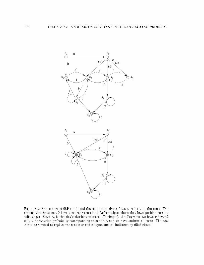
152 CHAPTER 7. STOCHASTIC SHORTEST PATH AND RELATED PROBLEMS
s s
s9
s9
e f
m
s8
s1 s2
a
cb
d
i
e f
gh
m
j
l
k
s s
ss
8
3
s s2
s6
7
5
b
h
c
a
i
l
1
s4
1 2
1/3
1/31/3
1/32/3
n
n
Figure 7.3: An instance of SSP (top), and the result of applying Algorithm 7.1 to it (bottom). Theactions that have cost 0 have been represented by dashed edges; those that have positive cost bysolid edges. State s9 is the single destination state. To simplify the diagrams, we have indicatedonly the transition probability corresponding to action c, and we have omitted all costs. The newstates introduced to replace the zero-cost end components are indicated by �lled circles.

7.2. THE NON-POSITIVE SSP PROBLEM 153
and replaces them with the two new states bs1 and bs2. This example illustrates also the potential
reduction of the state-space of the system.
The following theorem present the �rst approach to the solution of non-negative stochastic short-
est path problem.
Theorem 7.1 (non-negative SSP solution, approach 1) Consider an instance � of SSP sat-
isfying SSP Assumptions 3 and 4, and let b� be the instance obtained from � using Algorithm 7.1.
Then, b� satis�es SSP Assumptions 1 and 2, so that it can be solved using Theorem 3.4. Moreover,
it is
s 2 S
n[i=1
Bi : v�s = bv�ss 2 Bi; 1 � i � n : v�s = bv�si ;
where bv� (resp. v�) is the solution of b� (resp. �).
The second approach is given by the following theorem.
Theorem 7.2 (non-negative SSP solution, approach 2) Consider an instance � of SSP satis-
fying SSP Assumptions 3 and 4, and let L be the operator de�ned as in (3.8). Then, the solution v�
of the SSP problem is the largest �xpoint of operator L. Moreover, the linear programming problem
(3.9) has v� as unique solution.
7.2 The Non-Positive SSP Problem
Consider an instance (S;A; p; U; c; g) of the stochastic shortest path problem. We replace SSP
Assumptions 1 and 2 with the following assumptions:
SSP Assumption 3: There is at least one SSP-proper policy.
SSP Assumption 6: For all s 2 S and a 2 A(s), it is c(s; a) � 0. For all s 2 U , it is g(s) � 0.
An SSP problem that satis�es SSP Assumptions 3 and 6 is called a non-positive SSP problem. SSP
Assumption 6 is exactly like SSP Assumption 4, except that we require non-positivity of the costs
instead of non-negativity.
Denote as usual the optimal cost vector by v�. Unlike in the non-negative case, it is possible
that v�s = �1 for some state s 2 S � U . Our �rst step towards the solution of non-positive SSP
problems consists in determining the set of states on which v� diverges to �1.
Lemma 7.1 (divergence of optimal cost of non-positive SSP) Let
C =[n
B0��� 9(B;D) 2 maxEC (S � U) : 9(s; a) 2 sa(B;D) :
hB0 = B ^ c(s; a) < 0
io

154 CHAPTER 7. STOCHASTIC SHORTEST PATH AND RELATED PROBLEMS
and let bC be the set of states that can reach C. Then, v�s = �1 i� s 2 bC.Since states in S � bC cannot reach bC , in light of the previous lemma we continue our study of
non-positive SSP by adding one more assumption.
SSP Assumption 7: Every end component (B;D) of S�U is such that c(s; a) = 0 for all (s; a) 2
sa(B;D).
Clearly, if the above assumption does not hold, Lemma 7.1 enables to eliminate the o�ending
end components, along with the states that lead to them.
As in the previous section, the functional L de�ned by (3.8) can have more than one �xpoint,
and the solution of the SSP problem corresponds to the largest �xpoint. This is due to the fact that
there can be end components contained in S�U consisting of state-action pairs that all have cost 0.
Again, there are two approaches to the solution of non-positive SSP problems: one consists in
using Algorithm 7.1 to eliminate the o�ending end components, insuring that the functional on the
resulting instance of SSP problem has only one solution. As before, this opens the way to the use
of linear programming as well as other methods for the solution of the SSP instance. The second
approach consists in reducing the problem to linear programming directly. The two approaches are
summarized by the two following theorems.
Theorem 7.3 (non-positive SSP solution, approach 1) Consider an instance � of SSP sat-
isfying SSP Assumptions 3, 6 and 7, and let b� be the instance obtained from � using Algorithm 7.1.
Then, b� satis�es SSP Assumptions 1 and 2, so that it can be solved using Theorem 3.4. Moreover,
it is
s 2 S
n[i=1
Bi : v�s = bv�ss 2 Bi; 1 � i � n : v�s = bv�si ;
where bv� (resp. v�) is the solution of b� (resp. �).
Theorem 7.4 (non-positive SSP solution, approach 2) Consider an instance � of SSP satis-
fying SSP Assumptions 3 and 4, and let L be the operator de�ned as in (3.8). Then, the solution v�
of the SSP problem is the largest �xpoint of operator L. Moreover, the linear programming problem
(3.9) has v� as unique solution.
7.3 Proof of the Results for Non-Negative SSP (z)
Consider an instance � = (S;A; p; U; c; g) of SSP problem that satis�es SSP Assumptions 3 and 4.
To simplify the argument, we assume that once the set U of destination states is entered, it cannot

7.3. PROOF OF THE RESULTS FOR NON-NEGATIVE SSP 155
be exited. Formally, this is expressed by the requirement Succ(s; a) � U for all s 2 U and a 2 A(s).
It is immediate to see that this assumption does not a�ect the generality of the arguments.
As our �rst step towards the proof of Theorem 7.1, we show that a �xpoint of L provides a lower
bound for the solution v�. The following theorem is the analogous of Theorem 3.9.
Theorem 7.5 (�xpoint is below solution) If v� = Lv�, then v�s � v�s for every � 2 �P and
every s 2 S � U .
Proof. From v� = Lv�, it is
v�s � c(s; a) +X
t2S�U
pst(a) vt +Xt2U
pst(a) g(t)
for all s 2 S � U and all a 2 A(s). Iterating, for a general policy � and n � 0 we obtain
v�s � E�s
�n�1Xk=0
c(Xk; Yk)
�+
Xt2S�U
Pr�s(Xn = t) v�t +Xt2U
nXk=1
Pr�s(Xn = t ^ TU = k) g(t) : (7.1)
If � 2 �P , it is
limn!1
Xt2S�U
Pr�s(Xn = t) = 0 :
Taking the limit n!1 in (7.1), we have
v�s � E�s
� TUXk=0
c(Xk; Yk)
�+E�s
ng(XTU )
o;
which �nally yields v�s � v�s , as desired.
We can now prove our main result.
Proof of Theorem 7.1. The proof of this theorem follows closely that of Theorem 3.8. Again,
we break up the transformation e�ected by Algorithm 7.1 in two steps, and we consider an in-
stance (S; eA; ep; U;ec; eg) of SSP problem obtained as follows. Let (B1; D1); : : : ; (Bn; Dn) be as in
Algorithm 7.1, and de�ne
eA(s) =(fhs; ai j a 2 A(s)g if s 62
Sni=1 Bi;
fht; ai j t 2 Bi ^ a 2 A(t)�Di(t)g if s 2 Bi, 1 � i � n.(7.2)
and
epsu(ht; ai) = ptu(a) ec(s; ht; ai) = c(t; a) eg(s) = g(s) (7.3)
for all s; u 2 S and ht; ai 2 eA(s).

156 CHAPTER 7. STOCHASTIC SHORTEST PATH AND RELATED PROBLEMS
Let eL be the operator de�ned for e� in the same way as L for �, and let v� = eLv� be a �xpointof eL.
Note that e� satis�es SSP Assumption 1 and 2. The fact that the �rst one holds is a consequence
of SSP Assumption 3. To see that SSP Assumption 2 holds, note that for every end component
(B;C) in S � U there is (s; a) 2 sa(B;C) such that c(s; a) > 0: in fact, the end components
consisting only of state-action pairs with c = 0 have been eliminated by the transformation that led
to e�. Thus, for a Markovian policy � there are only two cases:
� Under �, a behavior reaches U with probability 1 from all s 2 S � U .
� Under �, there is an end component (B;C) with B � S�U such that Pr�s(inft(!) = sa(B;C)) >
0. Then, for these states it is also v�s =1, from the above considerations.
This shows that SSP Assumption 2 is satis�ed. We can then prove the following facts.
Fact 1. If v� = eLv� is a �xpoint of eL, and s; t 2 Bi, for 1 � i � n, then v�s = v�t .
Proved as in the proof of Theorem 3.8.
Fact 2. If v = eLv, then v = Lv.
This fact is proved as in the proof of Theorem 3.8, noting for (3.20) that c(s; a) = 0, for s 2 Bi,
a 2 Di(s) and 1 � i � n, by construction of the end components.
Our third fact follows from Theorem 3.4, which can be applied since the SSP problem e� satis�es
SSP-assumptions 1 and 2.
Fact 3. There is exactly one v� such that v� = eLv�.The equation v� = eLv�, written in componentwise notation, is
v�s = mina2eA
�c(s; a) +
Xt2S�U
epst(a) v�t +Xt2U
epst(a) g(t)�
s 2 S � U : (7.4)
From the �xpoint v� of eL we again construct a policy e� for e�. To this end, for each s 2 S � U ,
de�ne the set Amin(s) by
Amin(s) = argmina2eA
�c(s; a) +
Xt2S�U
epst(a) v�t +Xt2U
epst(a)g(t)�: (7.5)
At each s 2 S � U , policy e� chooses deterministically an arbitrary action selected from Amin(s).
For each 1 � i � n, from Fact 1 it is Amin(s) = Amin(t) for all s; t 2 Bi. Thus, we can force e� to
choose the same action hui; aii at all states of Bi. By Theorem 3.4, policy e� is SSP-proper, and it
is ve� = v�.
From e�, we construct a Markovian policy � for � such that v� = ve� . At s 2 S �
Sni=1Bi, �
behaves like e�. At s 2 Bi, with 1 � i � n, there are two cases:

7.4. PROOF OF THE RESULTS FOR NON-POSITIVE SSP 157
� if s = ui, then � chooses deterministically ai;
� if s 6= ui, then � chooses with uniform probability an action from the set Di(s).
From the de�nition of �, we see that � is SSP-proper. Proceeding as in the proof of Lemma 3.4, we
have that the system of equations
vs = c(s; �(s)) +X
t2S�U
epst(�(s)) vt +Xt2U
epst(�(s)) g(t) s 2 S � U (7.6)
has v� as unique solution. To show that ve� = v�, it su�ces to show that ve� is also a solution of
(7.6). The proof proceeds by cases.
� If s 2 Bi for 1 � i � n, and s 6= ti (where hti; aii is the action chosen by e� ), then policy �
chooses with uniform probability an action from Di(s). For a 2 Di(s), it is c(s; a) = 0 and
Succ(s; a) � Bi. From Fact 1, ve� = v� is constant on Bi, so v
e�s = v
e�t for a 2 Di(s) and
t 2 Succ(s; a), and the result follows.
� If s 2 Bi and s = ti, for 1 � i � n, or if s 2 Sr �Sni=1 Bi, policies � and e� coincide on s. The
fact that ve� satis�es (7.6) for s is then a consequence of ve� = v� and of (7.4), as well as of the
fact that e� chooses at s an action in Amin(s).
Since ve� = v�, it is also v� = v
�, and from Fact 2 we have v� = v� = Lv� . By Theorem 7.5, policy
� realizes the minimum cost, so that v� = v�.
The proof is then completed in analogy to that of Theorem 3.8, by noting that MDP b� is obtained
from e� by merging the states belonging to each Bi, for 1 � i � n.
Proof of Theorem 7.2. By Theorem 7.5, if v� = Lv�, then v� � v� for every � 2 �P , where the
inequality is interpreted componentwise.
From the proof of Theorem 7.1, we know that there is a policy � for � such that v� = v�. From
this follows immediately that v� � v� for all �xpoints v� of L. We conclude that v� is the maximal
�xpoint of L. The result about the reduction to linear programming is an immediate consequence
of this fact.
7.4 Proof of the Results for Non-Positive SSP (z)
First, we prove the following lemma, which is equivalent to one of the two directions of Lemma 7.1.
Lemma 7.2 Assume that there is an end component (B;D) in S � U such that c(t; a) < 0 for
at least one state-action pair (t; a) 2 sa(B;D). Assume also that B is reachable from s. Then,
v�s = inf�2�Pv�s = �1.

158 CHAPTER 7. STOCHASTIC SHORTEST PATH AND RELATED PROBLEMS
Proof. Since (B;D) is an end component reachable from s, there is a policy � such that
Pr�s (inft(!) = sa(B;D)) > 0. Since c(t; a) < 0 for at least one state-action pair (t; a) 2 sa(B;D),
it is v�s = �1. The problem is that policy � is not SSP-proper, since under it a behavior from s is
eventually con�ned to B with positive probability.
To overcome this di�culty, we construct a family of policies �(x), for 0 � x � 1, in such a way
that as x! 0 a behavior from s stays longer and longer in (B;D) before eventually reaching U .
To construct this family of policies, denote by bB � S�U the set of states that can reach B, and
let �m, �c and �p be three Markovian policies de�nes as follows:
� �m is a policy de�ned on bB �B that maximizes the probability of reaching B.
� �p is an SSP-proper Markovian policy. From SSP Assumption 3, we know that there is at least
one such policy, not necessarily Markovian; it can be easily seen, using reachability arguments
for U , that there is also at least one Markovian SSP-proper policy.
� �c is the policy de�ned on B that chooses at each s 2 B an action from D(s) with uniform
probability.
Using these three policies, for each 0 � x < 1 we de�ne the Markovian policy �(x) as follows:
Q�(x)(a j s) =
8>><>>:(1� x)Q�c(a j s) + xQ�p(a j s) if s 2 B;
(1� x)Q�m(a j s) + xQ�p(a j s) if s 2 bB �B;
Q�p(a j s) if s 2 S � bB.For every 0 < x < 1, policy �(x) is SSP-proper: in fact, it has non-zero probability of reaching U
in at most jS �U j steps from each state of S �U . Denote by P (x) the matrix of the Markov chain
corresponding to �(x), for 0 � x < 1, and abbreviate v�(x)s by vs(x). By de�nition, it is
vs(x) = E�(x)s
�TU�1Xk=0
c(Xk; Yk)
�+E�(x)s
ng(XTU )
o: (7.7)
De�ne two vectors z(x) = [zs(x)]s2S and u = [us]s2S by
zs(x) =
8><>:E�(x)s
�TU�1Xk=0
c(Xk; Yk)
�if s 2 S � U ;
0 otherwise;
us =
8<:
1
2jD(s)j
Xa2D(s)
c(s; a) if s 2 B;
0 otherwise.
For all s 2 S, it is us � 0. Since at least one state-action pair of (B;D) has c < 0, we know that
ut < 0 for at least one t 2 B. Since u represents only part of the negative cost incurred by a policy

7.5. THE MINIMUM EXPECTED TOTAL COST PROBLEM 159
that chooses in B with uniform probability the actions in D, for su�ciently small x it is
z(x) �
1Xk=0
P k(x)u : (7.8)
Since B is a closed recurrent class of the Markov chain corresponding to P (0), and since B is
reachable with positive probability from s, we have
� 1Xk=0
P k(0)u
�s
= �1 ;
where the notation [�]s indicates that we are considering the component of the vector corresponding
to s. From the continuity of P (x) in x = 0 follows limx!0 Pk(x) = P k(0) for all k � 0; thus,
limx!0
� 1Xk=0
P k(x)u
�s
= �1 ;
and hence from (7.8) and (7.7) we have limx!0 vs(x) = �1, which concludes our argument.
With this result, we can prove Theorem 7.3 and conclude the proof of Lemma 7.1.
Proof of Theorem 7.3. Consider an instance � of SSP satisfying SSP Assumptions 3, 6 and 7,
and let b� be the instance obtained from � using Algorithm 7.1. By SSP Assumptions 6 and 7, if
(B;D) is an end component of S � U , it must be c(s; a) = 0 for all (s; a) 2 sa(B;D). Since these
end components are eliminated by Algorithm 7.1, the resulting instance b� will not contain any end
component in S � U . Thus, all policies for b� are proper, and SSP Assumptions 1 and 2 hold. The
fact that the solutions of the SSP problem b� also provide solutions for � can then be proved by
reasoning as in the proof of Theorem 7.1.
Proof of Lemma 7.1. The �rst direction of the lemma was given in Lemma 7.2. In the other
direction, assume that in the instance � of SSP there is no end component (B;D) of S � U having
c(s; a) < 0 for some (s; a) 2 sa(B;D). The fact that vs > �1 at every s 2 S � U follows from
Theorem 7.3, and from the analysis of the SSP problem b� given in Section 3.4.
Theorem 7.4 can then be proved by repeating the argument used for Theorem 7.2.
7.5 The Minimum Expected Total Cost Problem
Even though the operator L can admit more than one �xpoint for non-negative and non-positive
instances of SSP problems, these instances can still be solved by a direct translation into linear

160 CHAPTER 7. STOCHASTIC SHORTEST PATH AND RELATED PROBLEMS
programming of the equation v = Lv, as indicated by Theorems 7.2 and 7.4 (albeit a more e�cient
solution is provided by Theorems 7.1 and 7.3).
In this section, we will describe instead a problem for which the straightforward reduction to
linear programming does not work: the non-negative minimum expected total cost (non-negative
METC) problem. Strauch [Str66] discusses this problem, and Denardo [Den70] proposed reductions
to linear programming that �nds bias-optimal policies for the METC problem without requiring
the non-negativity assumption. The proposal of [Den70] requires the solution of three nested linear
programming problems.
For the case of the non-negative METC problem we propose an alternative method, which re-
quires the solution of only one linear programming problem. Our method is based on a reduction
from the non-negative METC problem to the SSP problem. Aside from linear programming, the
reduction enables the use of value and policy iteration methods to solve non-negative METC prob-
lems.
The proposed reduction relies once more on the properties of end components. In fact, there
is a correspondence between the method of [Den70] and our proposal: the solution of some linear
programming problems in [Den70] corresponds to the removal of end components in our approach.
A discussion of the relationship between the two methods, however, is beyond the scope of this
dissertation.
The results developed in this subsection will not be used in the remainder of this dissertation,
and have been included due to their general interest only.
An instance of the METC problem is de�ned as follows.
De�nition 7.1 (minimum expected total cost problem) An instance of the minimum ex-
pected total cost problem consists of an MDP � = (S;A; p; c), in which c is a cost function assigning
to each state-action pair (s; a) 2 �� a cost c(s; a) 2 IR.
The METC problem consists in minimizing the total expected cost, over the set of all policies.
For a policy �, we de�ne the cost u�s of � from s 2 S by
u�s =
1Xk=0
c(Xk; Yk) : (7.9)
Note that the cost can be unbounded for some policies and initial states. The METC problem is
formally de�ned as follows.
De�nition 7.2 (minimum expected total cost problem) Given an instance � = (S;A; p; c)
of METC, determine
u�s = inf�u�s
for all s 2 S.

7.5. THE MINIMUM EXPECTED TOTAL COST PROBLEM 161
2 0s
ss
ss
3
4
0
1
0
3
5
4
2
1
Figure 7.4: An instance of non-negative METC. The actions are all deterministic, and the edgesare labeled with their cost. The end component composed by the states fs3; s4; s5g along with thezero-cost actions from these states is depicted using dashed lines.
We will provide a solution for the METC problem under the non-negativity assumption:
METC Non-Negativity Assumption: For all (s; a) 2 ��, it is c(s; a) � 0.
There is also a reduction from non-positive METC to SSP, albeit the reduction is more involved.
We will not discuss this reduction here, since the non-positive METC problem can also be solved
e�ciently with the methods discussed, for example, by Puterman [Put94].
Before presenting our reduction, let us gain some intuition into why the standard approach fails.
The Bellman equation for the METC problem can be written as u = Lu, where u = [us]s2S is the
cost vector, and the functional L is de�ned by
[Lu]s = mina2A(s)
�c(s; a) +
Xt2S
pst(a)ut
�: (7.10)
The operator L may have more than one �xpoint. As discussed in [Put94], u� is the least non-
negative �xpoint of L. The following example illustrates the presence of more than one �xpoint.
Example 7.4 Consider the instance of non-negative METC depicted in Figure 7.4. The operator
L de�ned in (7.10) admits in�nitely many �xpoints: two such �xpoints are u(1) and u(2), where
u(1)s1 = 5; u(1)s2 = 7; u(1)s3 = 3; u(1)s4 = 3; u(1)s5 = 3
u(2)s1 = 2; u(2)s2 = 4; u(2)s3 = 0; u(2)s4 = 0; u(2)s5 = 0
For this instance of METC, all �xpoints of L can be written in the form u(1) + x1, where x 2 IR
and 1 is the vector composed of jSj 1s. Vector u(2) is the least non-negative �xpoint of L, so that
by the arguments discussed in [Put94] it is u(2) = u�.

162 CHAPTER 7. STOCHASTIC SHORTEST PATH AND RELATED PROBLEMS
The problem of �nding the least non-negative �xpoint of L cannot be solved directly by linear
programming. In fact, the linear programming problem that arises directly from u = Lu is:
MaximizePs2S us subject to:
us � c(s; a) +Xt2S
pst(a)ut ; s 2 S; a 2 A(s) :
However, instead of �nding the least non-negative �xpoint of L, this linear programming problem
would �nd the largest such �xpoint. As noted in Example 7.4, this largest �xpoint can be unbounded.
From the example, we also see that the presence of multiple �xpoints is connected with the
existence of end components composed of state-action pairs having cost 0. Our analysis of the non-
negative METC problem exploits the existence of such end components. Our �rst result characterizes
the set of states on which u� <1. Given an instance � = (S;A; p; c) of METC, de�ne D(s) = fa 2
A(s) j c(s; a) = 0g, and let
S0 =[n
B��� (B;C) 2 maxEC (S;D)
o:
De�ne also
S<1 =ns 2 S
��� max�
Pr�s (reach(S0)) = 1o:
Theorem 7.6 The following assertions hold:
� If s 2 S0, then v�s = 0.
� v�s <1 i� s 2 S<1.
Proof. The �rst assertion is an immediate consequence of our results on end components.
For the second assertion, assume �rst that max� Pr�s (reach(S0)) < 1, and consider an arbitrary
policy �. Since the behaviors from s with probability 1 eventually follow and end component, there
must be an end component (B;C) such that:
� there is (t; a) 2 sa(B;C) such that c(t; a) > 0;
� Pr�s(inft(!) = sa(B;C)) > 0.
From these two statements, and from the fact that � is arbitrary, it follows immediately that u�s =1.
In the other direction, from our results on the maximum reachability probability problem we
know that there is a Markovian policy �m that maximizes the probability of reaching S0. Thus, if
s 2 S<1 it is max� Pr�ms (reach(S0)) = 1. From �m, reasoning as in the proof of Lemma 4.1 we can
obtain another Markovian policy �M , which coincides with �m outside S0, and that once in S0 it

7.5. THE MINIMUM EXPECTED TOTAL COST PROBLEM 163
follows forever one of the end components forming S0. Let P = [pst]s;t2S<1 , u = [u�Ms ]s2S<1 , and
c = [cs]s2S<1 , where
pst =X
a2A(s)
Q�M (a j s) pst(a) cs =X
a2A(s)
Q�M (a j s)c(s; a) :
Then, we can write u =P1k=0 P
kc. Noting that cs = 0 for s 2 S0, and that once S0 is entered, a
behavior never exits from S0, we can write bu =P1k=0
bP kbc, where bu, bP and bc are the restrictions ofu, P and c to S<1�S0. This is equivalent to bu = (I � bP )�1bc. Since bP is the matrix of a transient
Markov chain, det(I � bP ) 6= 0, and we conclude that bu is �nite. By de�nition of u�s , this implies
that u�s <1 for s 2 S<1.
It remains to compute the value of u�s at the states s 2 S<1 � S0. This can be done using
a straightforward reduction to the stochastic shortest path problem, as stated by the following
theorem.
Theorem 7.7 (reduction from non-negative METC to SSP) Consider the instance b� =
(S<1; bA; bp; S0;bc; g) of SSP problem, where bA and bp are the restrictions of A and p to S<1, bc is therestriction of c to S<1 � S0, and g is identically 0.
Then, the SSP problem satis�es SSP Assumptions 1 and 2. Moreover, it is u�s = v�s for all
s 2 S<1 � S0, where v�s denotes the solution of the SSP problem.
Proof. The fact that SSP Assumption 1 holds is a direct consequence of the de�nition of S<1. To
see that SSP Assumption 2 holds, we can reason as in the proof of Theorem 7.6 to show that if � is
SSP-improper, then v�s =1 for some s 2 S<1.
Denote by u, v the restrictions to S<1�S0 of the vectors corresponding to the cost of the METC
and SSP problems, respectively. As can be seen from the proof of Theorem 7.6, it is u� = inf�2�Pu� ,
i.e. the solution of the METC problem corresponds to an SSP-proper policy. For � 2 �P , it is
u� � v
� , since in the de�nition of METC, also the cost incurred after leaving the end components
in S0 is taken into account. Hence,
u� = inf
�2�P
u�� inf�2�
P
v� = v
� : (7.11)
In the other direction, if � is SSP-proper we can obtain another SSP-proper policy �0 that di�ers
from � only on S0, and such that �0 follows forever one of the end components of S0, once S0 is
entered. For this policy, it is v� = v�0 = u
�0 . Hence,
u� = inf
�2�P
u�� inf�2�
P
v� = v
� : (7.12)
The result follows by combining (7.11) and (7.12).

Chapter 8
Fairness
Fairness is a concept that has been widely used in the formal modeling and veri�cation of systems;
its traditional uses include the modeling of concurrency and of unbiased arbitration. In the context
of probabilistic systems, fairness serves also the additional purposes of abstracting from the speci�c
values of some transition probabilities, and of modeling transitions with an unspeci�ed distribution
of waiting times. The introduction of fairness in the system model requires the use of updated
speci�cation languages and model-checking algorithms, which will be described in this chapter.
The subject of fairness in probabilistic systems has been already discussed in the literature.
Pnueli [Pnu83] and Pnueli and Zuck [PZ93] introduce the notions of extreme fairness and �-fairness
to abstract from the precise values of probabilities. Hart, Sharir and Pnueli [HSP82] and Vardi
[Var85] consider probabilistic systems in which the choice of actions at the states is subject to
fairness requirements, and present algorithms for checking that temporal logic formulas hold with
probability 1 over these systems. This chapter has been inspired by Baier and Kwiatkowska [KB96],
which consider models very similar to Markov decision processes with fairness requirements, and
present algorithms to compute the probability with which temporal logic formulas hold over these
systems.
We return on the subject of fairness in probabilistic systems for three reasons. The �rst is to
introduce a notion of fairness that is better suited to the study of in�nite-state systems and to the
modeling of transitions with unknown delay distributions. The second is to propose a modi�cation
to the de�nition of the logics GPTL and GPTL* that leads to simpler model-checking algorithms.
The third reason is to provide model-checking algorithms for operators D, �P and �D, which have been
introduced in this dissertation.
We begin our presentation by brie y recalling a few notions of fairness that have been presented
in the literature, discussing the implications of each de�nition in the context of probabilistic systems.
We then introduce our version of fairness, called probabilistic fairness, and we present the temporal
logics FPTL and FPTL*, derived from GPTL and GPTL*. In these new logics, the semantics of
164

8.1. AN OVERVIEW OF FAIRNESS 165
the path quanti�ers and of the probabilistic operators is modi�ed to take into account the presence
of fairness. Finally, we describe the model-checking algorithm for FPTL and FPTL*, followed by
its correctness proof.
8.1 An Overview of Fairness
The concept of fairness in the context of formal system veri�cation was introduced by Lehmann,
Pnueli and Stavi [LPS81] for shared-variables programs, and by Queille and Sifakis [QS83] for tran-
sition systems. Its traditional uses include the modeling of concurrency and of un-biased arbitration;
among the monographs devoted to the study of fairness, we recall Francez [Fra86] and Apt, Francez
and Katz [AFK88].
Two notions of fairness are commonly considered: justice, also called weak fairness, and compas-
sion, also called strong fairness (see Manna and Pnueli [MP91, MP95]). Informally, the meaning of
justice and compassion can be described as follows. If � is a just or compassionate transition, then
every behavior of the system must obey the following constraints:
� � is just. If � is forever enabled, it must be taken in�nitely often.
� � is compassionate. If � is in�nitely often enabled, it must be taken in�nitely often.
Justice is mainly used to model the progress of individual threads of concurrent computation.
If all the transitions of a thread are just, then the execution of the thread must continue as long
as at least one of its transitions is enabled. Compassion is used to model fair choice, i.e. to model
probabilistic choice abstracting from the numerical values of the probabilities; it can be used in the
modeling of arbiters and message-passing systems.
In this dissertation, we will focus on probabilistic notions of fairness related to compassion, and
we will not propose methods for dealing with justice. In fact, compassion is better suited to model
unspeci�ed transition probabilities and unknown delay distributions, which are our motivations
for introducing fairness. We also remark that justice can be often substituted by the stronger
requirement of compassion, and that it would be possible to extend our de�nitions and algorithms
to encompass also the notion of justice.
8.2 Probabilistic Fairness
In a fair transition system, the fairness requirements are represented by specifying which transitions
are just and compassionate [MP91]. In the system model of timed probabilistic systems, the role
of transitions is played by actions. Di�erently from transition systems, however, we do not specify
fairness by a global set of fair actions: instead, we associate to each system state a set of actions that
are fair at that state. This approach is consistent with our desire to de-emphasize action names: the

166 CHAPTER 8. FAIRNESS
u v
b
ba
Figure 8.1: A fair Markov decision process � = (S;A; p;F), with S = fu; vg, A(u) = fa; bg,A(v) = fbg, F(u) = fa; bg, F(b) = ;. The probability distributions of the state-action pairs aredeterministic.
speci�cation of a global set of fair actions would assume an implicit correspondence between actions
at di�erent states that have the same name. The de�nition of fair Markov decision process is as
follows.
De�nition 8.1 (fair Markov decision process) A fair Markov decision process (FMDP) � =
(S;A; p;F) is a Markov decision process (S;A; p) with an additional labeling F that speci�es for
each s 2 S a subset F(s) � A(s) of fair actions at s.
A fair TPS (FTPS) is obtained from a TPS by adding the fairness labeling F , de�ned as for fair
MDPs.
De�nition 8.2 (fair TPS) A fair TPS � = (S;A; p;F ; Sin; time; I) consists of a TPS
(S;A; p; Sin; time; I) with an additional labeling F that is de�ned as for fair Markov decision pro-
cesses.
The fairness of an FTPS is enforced by de�ning a set of fair policies. Roughly, a policy is fair if
there is a global non-zero lower bound to the probability with which the fair actions are chosen. To
enforce the fairness requirements of a FMDP, we restrict our attention to fair policies in our de�nition
of logic and system semantics. This approach is closely related to that of [KB96], even though our
de�nition of fair policy is di�erent; we will later present a comparison of the two de�nitions.
De�nition 8.3 (fair policy) A policy � for an FMDP � = (S;A; p;F) is fair if there is � > 0
such that, for all n � 0, all sequences of states s0; : : : ; sn and all a 2 F(sn) it is Q�(a j s0 � � � sn) � �.
In the above de�nition, � can depend on the policy �, but cannot depend on the past sequence
s0 � � � sn of states, nor on the action a 2 F(sn). Thus, � represents a lower bound for the probability
with which � chooses any fair action throughout the behavior of the system. The following example
justi�es this de�nition.
Example 8.1 (past independence of �) Consider the FMDP depicted in Figure 8.1, and assume
that we adopt the following alternative de�nition of fair policy:

8.2. PROBABILISTIC FAIRNESS 167
A policy � for � = (S;A; p;F) is fair if, for all n � 0, all sequences of states s0; : : : ; sn
and all a 2 F(sn), it is Q�(a j s0 � � � sn) > 0.
Consider then the policy �� that, after the sequence s0; : : : ; sn, chooses the next action as follows:
� if sn = v, then �� chooses deterministically action b;
� if sn = u, then �� chooses a with probability pn = exp(�(2�n�1) log 2), and b with probability
1� pn.
According to the modi�ed de�nition, policy �� is fair, since the probability of choosing a and b at u
are always strictly positive. However, it is easy to check that a behavior that starts from s0 = u will
remain forever at u with probability 1=2. This clearly contradicts our intuitive notion of fair choice
between a and b, since a non-zero fraction of behaviors never chooses b, even though such a choice
is always possible.
To avoid this type of situation, De�nition 8.3 requires that the lower bound to the probability
of choosing a fair action is independent from the sequence of past states.
To gain a better understanding of the properties of our de�nition of fairness, we compare it with
other notions of fairness that have been proposed in the literature. To facilitate the comparison, we
have reformulated all de�nitions in terms of Markov decision processes, instead of introducing fair
transition systems, as in Manna and Pnueli [MP91], or probabilistic automata, as in Kwiatkowska
and Baier [KB96].
8.2.1 Compassion: Fair Transition Systems Approach
Consider an MDP (S;A; p), and let Acts be the underlying set of actions. Adapting the de�nition
of [MP91] to the notation of Markov decision processes, we represent FTS-compassion by a set
C � Acts of actions. Given a behavior ! : s0; a0; s1; a1; s2; : : :, we say that ! is FTS-fair if the
following condition holds for every a 2 C:
if a 2 A(si) for in�nitely many i � 0, then a = ai for in�nitely many i � 0.
Since the de�nition of [MP91] is not aimed at probabilistic systems, it does not specify how the
fairness of behaviors should be re ected in the set of policies that are considered. Two alternatives
appear to be the most natural, and have been explored by [KB96] in a similar setting:
� Only policies under which all behaviors are fair are considered.
� Only policies under which behaviors are fair with probability 1 are considered.
Clearly, the �rst alternative leads to a stronger de�nition of fairness than the second one. The
following example illustrates why the notion of FTS-compassion is not appropriate for our purpose of
abstracting from the value of transition probabilities, regardless of which one of the above alternatives
is chosen.

168 CHAPTER 8. FAIRNESS
b a
vu
s tc
c
ab
Figure 8.2: A Markov decision process � = (S;A; p) with S = fs; t; u; vg, and action sets as depicted.The probability distributions associated to all state-action sets are deterministic. To this MDP isassociated a set of compassionate actions C = fa; b; cg.
Example 8.2 Consider the MDP depicted in Figure 8.2, and consider the policy � de�ned by:
Q�(c j s) = 1 Q�(c j �ubs) = 1
Q�(c j �t) = 1 Q�(a j �tcs) = 1
Q�(b j �u) = 1 Q�(b j �v) = 1 ;
where � denotes any (possibly empty) sequence of alternated states and actions, and all other
conditional probabilities are 0. Intuitively, � chooses always b; b; c respectively at u; v; t; at s, it
alternately chooses a or c. Under �, every behavior is compassionate with respect to all actions,
since every action appears in�nitely often along every behavior. Nonetheless, action a is never
chosen at state t, indicating how this de�nition of compassion fails to capture fully the behavior of
probabilistic choice.
Extreme Fairness and �-Fairness
To remedy to the situation illustrated by the previous example, Pnueli [Pnu83] and Pnueli and Zuck
[PZ93] introduce the notions of extreme fairness and �-fairness. Similar concerns also led to the
concept of uniform compassion in Bj�rner, Lerner and Manna [BLM97].
The notion of �-fairness relies on the use of past temporal logic. Given a behavior ! =
s0a0s1a1s2 � � � and a past temporal formula �, we say that i � 0 is a �-position of ! if � holds
at position i of !. We say that an action a is taken at position i � 0 of ! if ai = a.
A behavior ! is �-fair with respect to � if, whenever a fair action a is enabled at in�nitely many
�-positions, a is chosen in�nitely often from �-positions. A behavior is �-fair if it is �-fair with
respect to all past temporal formulas.
This de�nition prevents situations such as the one discussed in Example 8.2 from arising. We

8.2. PROBABILISTIC FAIRNESS 169
ba b
ba b
ba b
(u,0)
(u,1)
(v,0)
(v,1)
(u,2) (v,2)
Figure 8.3: Markov decision process resulting from the \unrolling" of the process of Figure 8.1.
have preferred to base our results on the notion of probabilistic fairness rather than �-fairness
because the de�nition of probabilistic fairness does not require the introduction of past temporal
formulas, and because probabilistic fairness, being already stated in terms of probability, leads to a
simpler analysis of the model-checking algorithms.
8.2.2 State-Based Fairness
Baier and Kwiatkowska [KB96] propose a di�erent solution to the problem illustrated in Example 8.2.
According to [KB96], a behavior ! is fair if, whenever a state s appears in�nitely often along !,
all actions in A(s) also appear in�nitely often along !. This notion of fairness has its roots in the
state-fairness described in Pnueli [Pnu83] and Vardi [Var85]. As mentioned in [KB96], this de�nition
can be easily generalized to the case in which to each state s is associated a set of fair actions F(s).
A policy is strictly fair if under it all the behaviors are fair, and is (almost) fair if under it the
behaviors are fair with probability 1.
The drawback of this de�nition is that it does not directly apply to in�nite-state systems, as the
following example indicates.
Example 8.3 Consider the FMDP depicted in Figure 8.3. This FMDP can be obtained by taking
the product of the FMDP of Example 8.1 with an automaton over the natural numbers whose state
increases by one at each transition. Since no state of this MDP appears more than once in any
behavior, the fairness notion of [KB96] does not impose any constraint on the set of policies for it.
This example indicates that the de�nition of [KB96] is not invariant with respect to the product
with in�nite-state systems.
The notion of probabilistic fairness retains most of the properties of the proposal of [KB96] while
being readily extendible to in�nite-state systems. Moreover, probabilistic fairness is suited to the
representation of transitions with unknown delay distributions, as we will see in the next chapter.

170 CHAPTER 8. FAIRNESS
8.3 Time Divergence and Admissible Policies
In Chapter 3 we introduced the concept of non-Zeno TPSs: informally, a TPS is non-Zeno if time
diverges with probability 1 under any policy. In the previous chapters, we required that the TPSs
under consideration be non-Zeno, thus ensuring time divergence regardless of the policy.
While this approach leads to simpler logics and veri�cation algorithms, is not adequate for the
study of system approximations. A TPS that is constructed as the approximation of a system may
not be non-Zeno, since the substitution of probability with nondeterminism can lead to policies
under which time diverges with probability less than 1.
For these reasons, we adopt in the following a more general approach, due to Segala [Seg95b]. This
approach is based on the notion of time-divergent policies (called admissible in [Seg95b]): a policy
is time divergent if time diverges with probability 1 under it. While the non-Zenoness requirement
asks for all policies to be time divergent, the proposal of [Seg95b] is to consider the behavior of the
system only under time-divergent policies.
The advantage of the approach based on non-Zenoness is its simplicity: since in a non-Zeno TPS
all policies lead to time divergence, it is possible to de�ne the meaning of the probabilistic operators
by quantifying over the set of all policies, without distinguishing among time divergent and non-
divergent ones. However, our approach to fairness has already led us to restrict the set of policies
under consideration, so that adopting the approach of [Seg95b] does not complicate excessively the
semantics of the logic or the presentation of the model-checking algorithms. For this reason, in the
study of fair TPSs we adopt this approach, and we de�ne time divergent policies as follows.
De�nition 8.4 (time-divergent policy) Given an FTPS (S;A; p;F ; Sin; time; I), we say that
a policy � is time divergent for a state s if
Pr�s
� 1Xk=0
time(Xk; Yk) =1
�= 1 :
For each state s we de�ne the set Adm(s) of admissible policies for s as the set of policies that
are both fair and time divergent. This is the set of policies that will be considered in the logics and
veri�cation algorithms for fair TPSs.
De�nition 8.5 (admissible policy) We say that a policy � is admissible for a state s if � is both
fair and time divergent for s. The set of admissible policies for a state s is denoted by Adm(s). We
say that a policy � is admissible if it is admissible for all states.
Finally, we substitute Assumption 3.1 with the weaker assumption stating that every state has
at least one admissible policy.
Assumption 8.1 (admissibility) Given a fair TPS �, for every state s of � it is Adm(s) 6= ;.

8.4. PROBABILISTIC LOGICS FOR FAIRNESS: FPTL AND FPTL* 171
8.4 Probabilistic Logics for Fairness: FPTL and FPTL*
As a consequence of the introduction of fairness and of the new approach to time divergence, it
is necessary to provide new de�nitions for the semantics of the probabilistic temporal logics. The
new logics, called FPTL and FPTL* (from Fair Probabilistic Temporal Logics) are obtained from
GPTL and GPTL* by modifying the semantics of the path quanti�ers A, E and of the probabilistic
operators P, D, �P, �D. The rationale for the modi�cations is as follows.
8.4.1 Path Quanti�ers A, E
In GPTL or GPTL*, formula A� holds at a state s if all behaviors originating from s satisfy �.
Thus, the path quanti�ers A and E are de�ned as in CTL and CTL*.
This de�nition is not compatible with our approach to fairness. In fact, even if policy � is fair
and time divergent for s, some of the behaviors arising under � may not be fair, in the sense that
they may contain in�nitely many states where a fair action is possible, and contain only �nitely
many occurrences of that action. The behavior of the system under such unfair behaviors is taken
into account by the classical de�nition of the path quanti�ers, preventing the use of these quanti�ers
in speci�cations in which the fairness of the system matters.
The problem can be traced to the fact that, according to our de�nition, fairness is a restriction
on the probability distributions with which policies choose the actions, rather than a restriction on
the sequence of actions along every behavior. Hence, we are not able to guarantee that all behaviors
arising from a fair policy are fair in the classical sense: all we can guarantee is that they are fair
with probability 1. To remedy to this situation, we rede�ne the semantics of the path quanti�ers A
and E in FPTL and FPTL*. According to the our new de�nitions, formula A� holds at a state s if,
under any admissible policy, � holds with probability 1; the path quanti�er E is then de�ned as the
dual of A, as usual.
8.4.2 Operators P, D, �P, �D.
To simplify the model-checking algorithms, we adopt a new semantics for the probabilistic operators
P, D, �P, and �D. We motivate this choice by presenting the argument relative to the operator P;
similar arguments apply to the other operators.
Given a state s and a sequence formula �, denote by
P (s; �) =nx 2 [0; 1]
��� 9� 2 Adm(s) : Pr�s (! j= �) = xo
the set of values that the probability of � can assume under admissible policies. An analysis of
the algorithms presented in Baier and Kwiatkowska [KB96] (which are based on a di�erent notion
of fairness) reveals that determining supP (s; �) and inf P (s; �) can be done in time polynomial in

172 CHAPTER 8. FAIRNESS
the size of the TPS. Determining whether P (s; �) is open or closed at the endpoints, i.e. whether
inf P (s; �) 2 P (s; �) and supP (s; �) 2 P (s; �), requires more involved algorithms.
If supP (s; �) = a, determining whether P (s; �) is open or closed at the endpoints enables to
distinguish between the case in which P<a� holds at s, and the case in which only P�a� holds. We
note that the need to distinguish among these cases does not arise in the analysis of non-fair TPSs,
since the sets under consideration are closed at the endpoints in the absence of fairness. This is a
consequence of the existence of optimal policies that minimize or maximize the quantities measured
by P, D, �P and �D, a result that has been proved in the previous chapters.
Even in the case of fair TPSs, however, the practical usefulness of such a �ne distinction is open
to question, especially in view of fact that the transition probabilities of a system are known in many
cases only in an empirical fashion. In the logics FPTL and FPTL* we do not distinguish between
the cases in which P (s; �) is open or closed at the endpoints, and we base our de�nitions on the
supremum and in�mum of the set P (s; �) instead. This leads to simpler model-checking algorithms.
8.4.3 Semantics of FPTL and FPTL*
To de�ne the semantics of FPTL and FPTL*, we need to provide new de�nitions for the product of
a fair TPS and experiment, and for threshold outcomes. The product is de�ned as follows.
De�nition 8.6 (product of fair TPS and experiments) Given a fair TPS � =
(S;A; p;F ; Sin; time; I) and an experiment = (V;E;Er ; Vin; �), their product FMDP � =
� = (bS; bA; bp; bF ; dtime; r; w) is de�ned as in De�nition 5.5, with the addition that
bF(hs; vi) = F(s) dtime(hs; vi; a) = time(s; a)
for all hs; vi 2 bS and a 2 bA(hs; vi).Admissible threshold outcomes represent the minimum and maximum values for the long-run
average outcome of an experiment that can be attained with positive probability under an admis-
sible policy: they are the corresponding concept to threshold outcomes in presence of fairness (see
De�nition 5.9).
De�nition 8.7 (admissible threshold outcomes) Consider a fair TPS �, an experiment
and their product FMDP �. For each state hs; vi of �, we de�ne the maximum and minimum
threshold outcomes �FT+hs;vi and
�T�hs;vi by
�FT+hs;vi = sup
na 2 IR
��� 9� 2 Adm(hs; vi) : Pr�hs;vi
�I ^ lim sup
n!1Hn(!) � a
�> 0
o�FT�hs;vi = inf
na 2 IR
��� 9� 2 Adm(hs; vi) : Pr�hs;vi
�I ^ lim inf
n!1Hn(!) � a
�> 0
o;

8.4. PROBABILISTIC LOGICS FOR FAIRNESS: FPTL AND FPTL* 173
GPTL, GPTL* FPTL, FPTL*
s j= A� 8! 2 s : ! j= � 8� 2 Adm(s) : Pr�s (! j= �) = 1
s j= E� 9! 2 s : ! j= � 9� 2 Adm(s) : Pr�s (! j= �) > 0
s j= P./a� 8� : Pr�s(! j= �) ./ ahinf�2Adm(s) Pr
�s(! j= �)
i./ a
s j= D./a 8� : E�sftimeto( )g ./ ahinf�2Adm(s) E
�sftimeto( )g
i./ a
s j= �P./a 8� : Pr�hs;Vini
�I ! (lim supn!1Hn ./ a)
��FT�s () ./ a
s j= �D./a 8� : Pr�hs;Vini
�I ! (lim supn!1Hn ./ a)
��FT�s () ./ a
Table 8.1: Semantics of the path quanti�ers and probabilistic operators in GPTL, GPTL* andFPTL, FPTL*. The satisfaction relations in the left column holds if and only if the statements inthe two other columns hold. In the table, � denotes a sequence formula, a state formula, and an experiment. The formulas I and H appearing in the rows for �P and �D refer to the product withexperiment , and Vin is the initial vertex of �. The symbol a denotes either a non-negative realnumber (operators D, �D) or a real number in the interval [0; 1] (operators P, �P). The symbol ./denotes one of �; >: the de�nitions for �; < are analogous.
with the convention that, if Pr�hs;vi(I) = 0 for all � 2 Adm(hs; vi), then �FT
+hs;vi = �1, �FT
�hs;vi =
+1. For a state s of � we de�ne then
�FT+
s () =�FT
+
vin(s)�FT�s () =
�FT�vin(s)
:
Table 8.1 presents the de�nitions of the path quanti�ers and probabilistic operators in FPTL and
FPTL*. The table also gives the corresponding de�nitions in GPTL and GPTL*, for comparison.
The table uses the abbreviation
timeto( ) =
T �1Xk=0
time(Xk; Yk) : (8.1)
As usual, we say that a fair TPS satis�es a FPTL or FPTL* speci�cation � 2 Stat if all initial
states of the TPS satisfy �. The following de�nition is the exact counterpart of De�nition 4.1
De�nition 8.8 (validity over a fair TPS) Given a fair TPS � = (S;A; p;F ; Sin; time; I) and
an FPTL or FPTL* speci�cation � 2 Stat, we say that � satis�es �, written � j= �, i� s j= � for
all s 2 Sin.

174 CHAPTER 8. FAIRNESS
The following results states that operators A and E are the dual of each other in FPTL and
FPTL*. The result for GPTL and GPTL* was a consequence of the well-known result for CTL and
CTL*.
Theorem 8.1 (duality of path operators in FPTL, FPTL*) Given a state s and a sequence
formula � of FPTL or FPTL*, it is s j= A� i� s 6j= E:�, where the satisfaction relation j= is as
de�ned for FPTL and FPTL*.
8.5 Model-Checking Algorithms for FPTL and FPTL*
As usual, the model-checking problem for FPTL and FPTL* consists in determining the truth-value
of a given state formula � at all states of the system. As described in Chapter 4, this problem can be
solved by recursively evaluating the values of the state subformulas of � at all states of the system.
Since the only di�erence between FPTL, FPTL* and GPTL, GPTL* lies in the de�nition of the
path quanti�ers and the probabilistic operators, we need to provide model-checking algorithms only
for these operators. We present the model-checking algorithms for FPTL* only, since FPTL is a
subset of FPTL*.
We present the model-checking algorithms in this section, and their correctness proof in the next.
Before we proceed to stating the algorithms, we need some preliminary notions.
8.5.1 Admissible End Components
The concept of end components played a major role in the design and analysis of the model-checking
algorithms for GPTL and GPTL*. As explained in Chapter 3, this concept provided a characteri-
zation of the set of state-action pairs that could be repeated forever along a behavior with positive
probability. With the introduction of fairness in the system model and with the adoptions of the
approach of [Seg95b] to time divergence, we must revise this notion, and introduce admissible end
components (AECs). Admissible end components play the same role in the study of fair MDPs as
end components in the study of ordinary MDPs; they are de�ned as follows.
De�nition 8.9 (admissible end components) Given a fair MDP � = (S;A; p;F), an end
component (B;C) of � is admissible end component (AEC) if it satis�es the following two conditions:
� (fairness) for all s 2 B it is F(s) � C(s);
� (time divergence) there is (s; a) 2 sa(B;C) such that time(s; a) > 0.
Maximality and containment for AECs are de�ned as for end components.
Again, we introduce a shorthand to denote the set of AECs contained in a given sub-MDP.

8.5. MODEL-CHECKING ALGORITHMS FOR FPTL AND FPTL* 175
De�nition 8.10 (maxAEC ) Given a sub-MDP (B;C) of a fair MDP, we denote by
maxAEC (B;C) = f(D1; E1); : : : ; (Dn; en)g the set consisting of the maximal admissible end com-
ponents of (B;C). Moreover, we abbreviate maxAEC (B;AnB) by maxAEC (B).
Given a sub-MDP (C;D), the set of maximal admissible end components of (C;D) can be
computed using the following algorithm.
Algorithm 8.1 (computation of maximal admissible end components)
Input: A sub-MDP (C;D).
Output: The set L = maxAEC (C;D).
Initialization: J := f(C;D)g.
Repeat the following steps:
� Select (B;E) 2 J .
� For all s 2 B, let E0(s) := fa 2 E(s) j Succ(s; a) � Bg, and let
E00(s) :=
(E0(s) if F(s) � E0(s);
; otherwise.
� Let B1; : : : ; Bn be the strongly connected components of the graph (B; �(B;E00)), and let
Ei(s) = E00(s) for all i 2 [1::n] and s 2 Bi.
� Replace (B;E) 2 J with (B1; E1); : : : ; (Bn; En).
Until: J cannot be changed by the above iteration.
Return: L = f(B;E) 2 J j 9(s; a) 2 sa(B;E) : time(s; a) > 0g.
The following two theorems provide a characterization of admissible end components, and are
the counterparts of Theorems 3.1 and 3.2 of Chapter 3.
Theorem 8.2 (stability of AECs) Let (C;D) be an admissible end component. Then, for every
admissible policy � there is an admissible policy �0 such that:
Pr�s(reach(C)) = Pr�0
s (reach(C)) = Pr�0
s (inft(!) = sa(C;D)) (8.2)
for all s 2 S.
Proof. Policy �0 can be constructed from � as follows. After the past s0 � � � sn:
� if sn 62 C, then Q�0(a j s0 � � � sn) = Q�(a j s0 � � � sn) for all a 2 A(s);

176 CHAPTER 8. FAIRNESS
� if sn 2 C, then Q�0(a j s0 � � � sn) is equal to jD(s)j�1 if a 2 D(s), and is equal to 0 otherwise.
It is easy to verify that �0 is admissible, and that (8.2) holds for � and �0.
The following theorem states that, for any initial state and admissible policy, a behavior will
eventually follow with probability 1 an admissible end component.
Theorem 8.3 (fundamental theorem of admissible end components) For any s 2 S and
any admissible policy �, Pr�s(sub(inft(!)) is an AEC ) = 1.
Proof. The proof of this theorem follows the idea of the proof of Theorem 3.2. First, note that
with probability 1 the sub-MDP sub(inft(!)) is an end component. Since there are only countably
many end components, it remaints to be proved that if Pr�s (sub(inft(!)) = (C;D)) > 0 for an
end component (C;D), then (C;D) is admissible. Assume thus that � is admissible, and that
Pr�s(sub(inft(!)) = (C;D)) > 0.
Since � is admissible, there is a lower bound � to the probability of choosing an action in F(s)
at every state s. Thus, by reasoning in analogy with the proof of Theorem 3.2 it can be proved
that F(s) � D(s) for all s 2 C, which is our �rst requirement for (C;D) to be admissible. It is
then immediate to see that there must be at least one state-action pair (s; a) 2 sa(C;D) such that
time(s; a) > 0, due to the time-divergence requirement. This is the second requirement for (C;D)
to be admissible, and the proof is concluded.
8.5.2 Existence of Admissible Policies
The �rst task of the model-checking algorithms is to verify that Assumption 8.1 holds. We present
two algorithms. The �rst algorithm checks whether there is at least one admissible policy for every
state. The second algorithm enables to obtain, given a TPS �, the maximal sub-TPS �0 of � that
satis�es Assumption 8.1. The second algorithm is not necessary for model checking, but it can be
used in a pre-processing step to obtain a TPS that can be model-checked.
Algorithm 8.2 (checking Assumption 8.1)
Input: A fair TPS � = (S;A; p;F ; Sin; time; I).
Output: Yes/no answer indicating whether Assumption 8.1 holds for �.
Method: Let G = fs 2 S j 9a 2 A(s) : time(s; a) > 0g be the set of states from which time can
advance. Answer \yes" if every state of S can reach some state of G in the graph (S; �S), and
\no" otherwise.

8.5. MODEL-CHECKING ALGORITHMS FOR FPTL AND FPTL* 177
Algorithm 8.3 (computing the sub-TPS that satisfy Assumption 8.1)
Input: A fair TPS � = (S;A; p;F ; Sin; time; I).
Output: The (possibly empty) maximal sub-TPS �0 of � that satis�es Assumption 8.1.
Method:
� Let S0 = S, A0 = A.
� Repeat:
{ Let G = fs 2 S0 j 9a 2 A0(s) : time(s; a) > 0g.
{ Let B0 be the subset of states of S0 that cannot reach G in (S0; �(S0;A0)).
{ Remove from S0 all states in B0.
{ Repeat:
� Remove from S0 all states s 62 S� that have a fair action leading to at least one
removed state.
� Remove from A0 all the actions leading to at least one removed state.
� Remove from S0 all states s 62 S� that have no actions left in A0.
{ Until no more states or actions can be removed from S0, A0.
� Until no more states or actions can be removed from S0, A0.
� Let F 0, time0, I 0 be the restrictions of F , time, I to S0, A0, and output the fair TPS
�0 = (S0; A0; p0;F 0; S0 \ Sin; time0; I 0).
Note that the fair TPS �0 needs not be connected, nor it needs to contain any initial state. These
conditions can be tested after the application of Algorithm 8.3.
8.5.3 Path Quanti�ers
Given a fair TPS � = (S;A; p;F ; Sin; time; I) and a sequence formula �, we now present algorithms
to decide whether s j= A� and s j= E�. As in Section 4.4, we assume that the value of the maximal
state subformulas �1; : : : ; �n of � has already been evaluated at all states of the TPS. Again, we let
�0 = [r1=�1] : : : [rn=�n] to be the result of replacing each �i with a new propositional symbol ri, for
every t 2 S we de�ne its label l(t) by l(t) = fri j 1 � i � n ^ t j= �ig.
Let �:�0 = � DR:�0 be the MDP obtained by taking the product between the l-labeled
TPS � and the deterministic Rabin automaton DR:�0 for :�0. This product is computed as
in Algorithm 4.2. For each state s = ht; vi of �0 corresponding to states t of � and v of
DR:�0 , we let F0(s) := F(t), and for a 2 A(t) we also let time(s; a) := time(t; a). Let
U 0 = f(P 01; R
01); : : : ; (P
0m; R
0m)g be the acceptance list for �0. The following theorem enables to
decide whether s j= A�.

178 CHAPTER 8. FAIRNESS
Theorem 8.4 (model checking of A in FPTL, FPTL*) s j= A� i� there is no admissible
end component (C;D) reachable from hs; qini in �:�0 such that C � P 0i and C \ R0
i 6= ; for some
1 � i � m.
This theorem leads immediately to the following model-checking algorithm.
Algorithm 8.4 (model checking of A in FPTL, FPTL*)
Input: TPS � and sequence formula �.
Output: The set SA� = fs 2 S j s j= A�g.
Method: First, compute the MDP ��0 = (S0; A0; p0;F 0; U 0) as described above, and let
S:� =[n
B��� 9(P;R) 2 U 0 : 9(C;D) 2 maxAEC (P ) :
hB = C ^ C \ R 6= ;
io:
Then,
SA� =ns 2 S
��� hs; qini cannot reach S:� in (S0; �S0)o:
Since operators A and E are the dual one of the other, as stated by Theorem 8.1, the above
algorithm also provides a solution to the model-checking problem for the path quanti�er E.
8.5.4 Operator P
We provide an algorithm to check whether s j= P./a� holds, for 0 � a � 1 and ./2 f�; <g. The
other cases can be solved by exploiting the relations
s j= P>a� i� s j= P<1�a:�
s j= P�a� i� s j= P�1�a:�
which hold for FPTL and FPTL*, as it can be easily shown. While it is possible to use the algorithms
of this subsection (taking a = 0 or 1) to obtain model-checking algorithms for A and E, the algorithms
presented in the preceding subsection are more e�cient, since they avoid the reduction to linear
programming that is necessary for the case 0 < a < 1.
Given a fair TPS � = (S;A; p;F ; Sin; time; I) and a sequence formula � of FPTL or FPTL*, let
�0 be the result of replacing the maximal state subformulas in � with propositional symbols, as in
the previous subsection, and let
�� = (S0; A0; p0;F ; time; U 0) = �DR�0
be the MDP obtained by taking the product between the l-labeled TPS � and the deterministic
Rabin automaton DR�0 , and adding the F and time labels as described in the algorithm for path

8.5. MODEL-CHECKING ALGORITHMS FOR FPTL AND FPTL* 179
quanti�ers. The following theorem is the analogous of Theorem 4.2, and provides an algorithm for
the model checking of operator P in FPTL and FPTL*. This algorithm is very similar to the one
presented in [KB96, Section 10] (which in turn is based in part on [BdA95, dA97]). The similarity
of the algorithms is in spite of the fact that the de�nition of fairness, and other details of the system
models, are di�erent.
Theorem 8.5 (model-checking of P in FPTL and FPTL*) Let
S� =[n
B��� 9(P;R) 2 U 0 : 9(C;D) 2 maxAEC (P ) :
hB = C ^ C \ R 6= ;
io:
Then,
sup�2Adm(s)
Pr�s(�) = max�
Pr�hs;qini
(reach(S�)) ;
where the rightmost reachability probability is computed in �� over the set of all possible policies.
8.5.5 Model Checking D./a for ./2 f�; <g
The model checking of operator D is based on a reduction to the stochastic shortest path problem,
as was the case for GPTL and GPTL*. The reduction used for FPTL and FPTL* is more complex,
due to the presence of fairness and to the approach adopted to the problem of time divergence. We
present �rst the case in which the inequality operator used as subscript of D is � or <.
Consider a fair TPS � = (S;A; p;F ; Sin; time; I), and let D./a� be the formula to be model
checked, where � is a state formula of FPTL or FPTL*, ./2 f�; <g and a � 0. As usual, we assume
that the truth value of � has already been evaluated at all states, and we let S� = fs 2 S j s j= �g.
The following lemma takes care of the states in S�.
Lemma 8.1 If s 2 S�, then s j= D./a�, for ./2 f�; <g and any a � 0.
Next, we consider the states in S � S�. To determine the subset of S � S� from which the
expected time to S� diverges, we reason as follows. Assume that there is an end component (B;C)
in S � S� containing at least one state-action pair (s; a) 2 sa(B;C) with time(s; a) > 0. Assume
also that (B;C) is reachable from s without leaving S � S�. Then, there is an admissible policy
that reaches (B;C) from s with positive probability. If (B;C) is an admissible end component,
this admissible policy can force any behavior that reaches (B;C) to remain in (B;C) forever, thus
causing the expected time to S� from s to diverge. Even if (B;C) is not admissible, however, we
can construct a sequence �0; �1; : : : of admissible policies that, once in (B;C), leave (B;C) with
probability at most �0; �1; : : :, with limn!1 �n = 0. These policies spend an expected amount of
time in (B;C) that diverges as n ! 1; the expected time from s to S� will also diverge. These
considerations lead to the following result.

180 CHAPTER 8. FAIRNESS
Theorem 8.6 Let
B =[n
B0��� 9(C;D) 2 maxEC (S � S�) : 9(s; a) 2 sa(C;D) :
hB0 = C ^ time(s; a) > 0
io;
and let bB be the subset of S�S� consisting of the states that can reach B in the graph (S�S�; �S�S�).
For s 2 bB, ./2 f�; <g and any a � 0, it is s 6j= D./a�.
We must still compute the truth value of D./a� at the states in C = S � (S� [ bB). To do
so, we construct an instance of SSP problem (C [ S�; A; p; S�; c; g) where the cost c is de�ned by
c(s; a) = �time(s; a) for all s 2 C and a 2 A(s), and g is identically 0. Note that we have slightly
abused the notation, since in this instance there can be actions leading from S� outside of C [ S�.
However, since the transition structure in S� plays no role in the SSP problem, this abuse of notation
has no ill consequences.
Let v�s = inf�2�Pv�s , as usual. The following theorem establishes the connection between the
solution of this instance of SSP problem and the model checking of D./a.
Theorem 8.7 For s 2 C, let v�s be the solution of the SSP problem mentioned above. Then,
s j= D./a� i� � v�s ./ a ;
for s 2 C, a � 0 and ./2 f�; <g.
Di�erently from Section 4.5.1, we cannot use the results of Bertsekas and Tsitsiklis [BT91] to
solve this instance of SSP problem, since SSP Assumption 2 does not necessarily hold. In fact, we
cannot rule out the presence of an end component (B;D) in C such that time(s; a) = 0 for all s 2 B,
a 2 D(s). In Section 4.5.2, the existence of such end components was ruled out by the non-Zenoness
requirement. This instance of SSP problem can nonetheless be solved with the results of Section 7.2.
8.5.6 Model Checking D./a for ./2 f�; >g
Similarly to the case of GPTL and GPTL*, the �rst step in the model checking of D./a� consists
in computing the sub-MDP consisting of the states that can reach S� with probability 1 under an
admissible policy. The following algorithm is the analogous of Algorithms 3.2 and 8.3.
Algorithm 8.5
Input: TPS � and set S�.
Output: The sub-MDP (S0; A0), where S0 = fs 2 S j max�2Adm(s) Pr�s(reach(S�)) = 1g, and A0 is
the restriction of A to S0.
Method:

8.5. MODEL-CHECKING ALGORITHMS FOR FPTL AND FPTL* 181
� Let S0 = S, A0 = A.
� Repeat:
{ Let B0 be the subset of states of S0 that cannot reach S� in the graph (S0; �(S0;A0)).
{ Remove from S0 all states in B0.
{ Repeat:
� Remove from S0 all states s 62 S� that have a fair action leading to at least one
removed state.
� Remove from A0 all the actions leading to at least one removed state.
� Remove from S0 all states s 62 S� that have no actions left in A0.
{ Until no more states or actions can be removed from S0, A0.
� Until no more states or actions can be removed from S0, A0.
� Output (S0; A0).
The following lemmas can be used to decide the value of D./a� at all states of (S � S0) [ S�.
Lemma 8.2 Given a state formula �, let S0 be as computed by Algorithm 8.5. If s 2 S � S0, it is
E�s
�T��1Xk=0
time(Xk; Yk)
�=1
for any policy �. Thus, for ./2 f�; >g, a � 0 and s 2 S � S0 it is s j= D./a�.
Lemma 8.3 If s 2 S�, then s j= D./a� i� both a = 0 and ./ is �.
We must still determine the truth value of D./a� at all states in C = S0 � S�. To do so, we
construct an instance of SSP problem (S0; A0; p; S�; c; g), where the cost c is de�ned by c(s; a) =
time(s; a) for all s 2 S0 � S� and a 2 A0(s), and g is identically 0. Note that this de�nition involves
again a slight abuse of notation, similarly to the construction of the SSP instance for Theorem 8.7.
Let v�s = inf�2�Pv�s , as usual. The following theorem establishes the connection between the
solution of this instance of SSP problem and the model checking of D./a.
Theorem 8.8 For s 2 C, let v�s be the solution of the SSP problem mentioned above. Then,
s j= D./a� i� v�s ./ a ;
for s 2 C, a � 0 and ./2 f�; >g.
As in the preceding subsection, we cannot use the results of Bertsekas and Tsitsiklis [BT91] to
solve this instance of SSP problem, since SSP Assumption 2 does not necessarily hold. Again, the

182 CHAPTER 8. FAIRNESS
reason is that we cannot rule out the presence of end components (B;D) in C such that time(s; a) = 0
for all s 2 B, a 2 D(s). This instance of SSP problem can nonetheless be solved with the results of
Section 7.1.
8.5.7 Operators �P and �D
The model checking of operators �P and �D in FPTL and FPTL* relies on an algorithm almost
identical to the one given for GPTL and GPTL* in Section 6.1.2. Let �0 = (S;A; p;F ; time;W;R)
be the result of computing the product between a TPS �0 and an experiment , as in De�nition 8.6,
and of substituting the r, w labels with the R, W ones.
The only di�erence between the algorithm for FPTL and FPTL* and the one presented in
Section 6.1.2 is that in the algorithm for FPTL and FPTL*, Step 1 is replaced by the following step:
1'. Compute the list L = f(S1; A1); : : : ; (Sn; An)g of maximal admissible end components of �0. For
each end component (Si; Ai), 1 � i � n, construct an MDP �i = (Si; Ai; pi; Ri;Wi), where p
i,
Ri, Wi are the restrictions of p, R, W to (Si; Ai).
The algorithm then proceeds as in Section 6.1.2.
8.6 Complexity of FPTL and FPTL* Model Checking
From an exam of the model-checking algorithms given in the previous sections, we can see that the
model-checking of FPTL and FPTL* speci�cations shares the same global complexity bounds of the
model-checking for GPTL and GPTL*.
Theorem 8.9 (complexity of FPTL, FPTL* model checking) Given a TPS �, the following
assertions hold:
� Checking whether � satis�es Assumption 8.1 has polynomial time-complexity in jj�jj.
� Model checking an FPTL formula � has time-complexity linear in j�j and polynomial in j�j.
� Model checking an FPTL* formula � has time-complexity doubly exponential in j�j and poly-
nomial in j�j.
A more detailed result is as follows.
Theorem 8.10 (complexity of FPTL, FPTL* model checking II) Assume that the truth of
all state subformulas of � has already been evaluated at all states. The following assertions hold:
� The model checking of A�, E� has the following time-complexity:
FPTL: Polynomial in jj�jj and independent of �.

8.6. COMPLEXITY OF FPTL AND FPTL* MODEL CHECKING 183
Logic
Operator GPTL GPTL* FPTL FPTL*
A, Epoly(jj�jj)indep(�)
poly(jj�jj)exp(j�j)
poly(jj�jj)indep(�)
poly(jj�jj)2-exp(j�j)
Ppoly(j�j)indep(�)
poly(j�j)2-exp(j�j)
poly(j�j)indep(�)
poly(j�j)2-exp(j�j)
Dpoly(j�j)indep(�)
poly(j�j)indep(�)
poly(j�j)indep(�)
poly(j�j)indep(�)
�P, �Dpoly(j�j)poly(jj)
poly(j�j)poly(jj)
poly(j�j)poly(jj)
poly(j�j)poly(jj)
Table 8.2: Complexity of the model-checking algorithms for the probabilistic logics considered inthis dissertation. In this table, we assume that the truth of all state subformulas of � has alreadybeen evaluated at all states. Symbol indicates an experiment. The symbol indepindicates that thecomplexity does not depend on that parameter; the symbols poly, exp and 2-exp indicate polynomial,exponential and doubly exponential complexities respectively. The case where the logics with andwithout fairness di�er has been indicated in boldface.
FPTL*: Polynomial in jj�jj and doubly exponential in j�j.
� The model checking of P./a� has the following time-complexity:
FPTL: polynomial in j�j and independent of j�j.
FPTL*: polynomial in j�j and doubly exponential in j�j.
� The model checking of D./a� has time-complexity polynomial in j�j and independent of �.
� The model checking of �P./a�, �D./a� for an experiment has time-complexity polynomial in
both j�j and j�j.
Proof. The lower bounds are a consequence of the results of Courcoubetis and Yannakakis [CY88];
the upper bounds are derived from an analysis of the proposed model-checking algorithms.
Table 8.2 summarizes the results on the complexity of the model-checking algorithms for the
probabilistic logics presented in this dissertation.

184 CHAPTER 8. FAIRNESS
8.7 Correctness Proof of Model-Checking Algorithms (z)
8.7.1 Policy Approximation
The computational part of the model-checking algorithms for FPTL and FPTL* relies on the solution
of optimization problems on Markov decision processes. These problems are solved in an uncon-
strained fashion, without placing any restriction on the policies, and the optimal policy or policies
may not be admissible. On the other hand, the semantics of the FPTL and FPTL* operators is
de�ned only in terms of admissible policies.
To justify the use of unconstrained solutions in FPTL or FPTL* model checking, we have to
show that the optimal values of the quantities of interest, such as probabilities or expected times,
can be realized or at least approximated by admissible policies. To this end, we use the notion
of approximation of non-admissible policies by admissible ones. This notion has been discussed in
Pnueli [Pnu83] and Kwiatkowska and Baier [KB96].
Informally, the idea is that it is sometimes possible to approximate a non-admissible policy with
a series of admissible ones, such that the quantity of interest (probability, expected time) for the
admissible policies can be made as close as desired to that of the non-admissible policy. We have
already seen this notion at work in the proof of Lemma 7.2. In this subsection, we present results
that will help to construct other approximability proofs.
Recall that a substochastic matrix is a matrix P = [pij ]1�i;j�N such that 0 � pij � 1 for all
1 � i; j � N andPNj=1 pij � 1 for all 1 � i � N [KSK66].
Theorem 8.11 (continuity of steady-state distributions) For a �xed N , consider a family
P (x) = [pij(x)]1�i;j�N of substochastic matrices parameterized by a parameter x 2 I, where I � IR
is an interval of real numbers. Assume that the Markov chain having P as transition matrix has the
same set of closed recurrent classes for all x 2 I. Then, if the coe�cients of P (x) depend continuously
on x for x 2 I, also the coe�cients of the steady-state matrix P �(x) depend continuously on x for
x 2 I.
Proof. The proof proceeds in stages, paralleling the classi�cation of states in a �nite Markov chain.
First, we consider each closed recurrent class separately. Assume that the matrix P corresponds
to a chain consisting in a single closed recurrent class. Then, the matrix P �(x) can be written
as P �(x) = 1�(x), where 1 is a column vector consisting of N 1s, and �(x) is the row vector
corresponding to the steady-state distribution of the chain. The row vector �(x) is the solution of
the equation
�(x)[P (x)1] = [�(x) 1] ; (8.3)
where [P (x)1] indicates the N � (N +1) matrix obtained by adjoining the column vector 1 to P (x),
and similarly [�(x) 1] is the row vector with N+1 elements obtained by adjoining a single 1 to �(x).

8.7. CORRECTNESS PROOF OF MODEL-CHECKING ALGORITHMS 185
Equation (8.3) is over-constrained: since the chain is composed of a single closed recurrent class,
any column of P (x) can be written as the linear combination of the others. Thus, in (8.3) we can
delete the columns corresponding to the �rst element, and determine �(x) by
�(x)[P]1(x)1] = [�]1(x) 1] ; (8.4)
where P]1(x) is the (N � 1) �N matrix obtained from P (x) by deleting the �rst column, and �]1
is the row vector of N � 1 elements obtained by deleting the �rst element of �(x). Equation (8.4)
can in turn be rewritten as
�(x)Q(x) = �(x)R + d ; (8.5)
where
Q(x) = [P]1(x)1] R = [�i�1;j ]1�i;j�N d = [00 � � � 0| {z }N�1
1]
and where �i;j = 1 if i = j and 0 otherwise. From (8.5), solving for �(x) we obtain
�(x) = d(Q(x) �R)�1 :
Since for x 2 I all states are in the same single closed recurrent class, this equation has a single
solution for all x 2 I , so that det(Q(x) � R) 6= 0 for x 2 I . If det(Q(x) � R) 6= 0, the coe�cients
of (Q(x) � R)�1 are continuous functions (in fact, rational functions) of the coe�cients of P (x).
Hence, the coe�cients of �(x) and those of P �(x) are continuous in x, for x 2 I .
Assume now that the Markov chain corresponding to P (x) has closed recurrent classes
C1; : : : CM � f1; : : : ; Ng for x 2 I . For 1 � i � N , call P �i (x) the i-th row of matrix P �(x).
Let C =SMj=1 Cj be the union of the closed recurrent classes, and T = f1; : : : ; Ng�C be the set of
transient states. For 1 � i � N , row P�i (x) can be written as
P�i (x) =
MXj=1
qji (x)�j(x) ; (8.6)
where �j(x) is the row vector corresponding to the steady-state distribution of class Cj , and qji (x)
is the probability of reaching Cj from i. If i 2 Ck, then qii(x) = 1 and qji (x) = 0 for all x 2 I and all
j 6= k.
For i 2 T , these probabilities are related by
qji (x) =
Xk2T
pik(x) qjk(x) +
Xk2Cj
pik(x)

186 CHAPTER 8. FAIRNESS
for 1 � j �M . In matrix form, this can be written as
Qj(x) = PT (x)Qj(x) +Rj(x) ;
where Qj = [qji (x)]i2T is a column vector, PT (x) is the restriction of P (x) to the transient states,
and Rj(x) = [rji (x)]i2T is de�ned by
rji =Xk2Cj
pik(x) :
Solving for Qj(x) we obtain
Qj(x) = (I � PT (x))�1Rj(x) : (8.7)
Since PT (x) is the matrix of a transient chain, det(I�PT (x)) 6= 0, and the coe�cients of (I�PT (x))�1
are continuous functions (in fact, rational functions) of x for x 2 I . From (8.6) and (8.7), and from
the previous part of the proof, we can thus conclude that the coe�cients of P �(x) are continuous in
x, for x 2 I .
A similar result holds for chains in which there is a single closed recurrent class, and there is a
state that is always in that class, for all values of the parameter. To state the result, we say that
a state is surely recurrent if the Markov chain has only one closed recurrent class, and the state
belongs to that class.
Theorem 8.12 For a �xed N , consider a family P (x) = [pij(x)]1�i;j�N of substochastic matrices
parameterized by a parameter x 2 I, where I � IR is an interval of real numbers. Assume that there
is a state 1 � k0 � N that is surely recurrent for all x 2 I. Then, if the coe�cients of P (x) depend
continuously on x for x 2 I, also the coe�cients of the steady-state distribution vector ��(x) depend
continuously on x for x 2 I.
Proof. This theorem can be proved similarly to the �rst part of the previous one. The row vector
�(x) is the solution of the equation
�(x)[P (x)1] = [�(x) 1] ; (8.8)
where [P (x)1] indicates the N � (N +1) matrix obtained by adjoining the column vector 1 to P (x),
and similarly [�(x) 1] is the row vector with N+1 elements obtained by adjoining a single 1 to �(x).
Equation (8.8) is over-constrained: since the chain has a single closed recurrent class, the columns
of P (x) that correspond to states in the class can be written as the linear combination of the other
columns. Thus, in (8.3) we can delete the column corresponding to k0, and determine �(x) by
�(x)[P]k0 (x)1] = [�]k0(x) 1] ; (8.9)

8.7. CORRECTNESS PROOF OF MODEL-CHECKING ALGORITHMS 187
where P]k0(x) is the (N � 1) � N matrix obtained from P (x) by deleting column k0, and �]k0 is
the row vector of N � 1 elements obtained by deleting the k0-th element of �(x). The proof is then
concluded in the same way as the previous one.
8.7.2 Model Checking of Path Quanti�ers
The proof of Theorem 8.4 is related to the results of Courcoubetis and Yannakakis [CY88, CY95]
relative to the problem of probabilistic emptiness. The di�erences lie in the presence of fairness, in
the concept of admissible policies, and in the use of Rabin automata and end components in the
analysis of the problem.
Proof of Theorem 8.4. Recall that a behavior ! of � satis�es :� i� there is 1 � i � n such that
inftst(!0) � Pi and inftst(!0) \ Ri 6= ;, where !0 is the behavior of �:� corresponding to !, and
inftst(!0) denotes the set of states occurring in�nitely often along !0.
If there is no admissible end component (B;C) reachable from hs; qini such that B � Pi and
B \ Ri 6= ; for some 1 � i � n, then from Theorem 8.3 we can conclude Pr�s(:�) = 0 for every
policy �, as desired.
Conversely, assume that there is an end component (B;C) reachable from hs; qini such that
B � Pi and B\Ri 6= ; for some 1 � i � n. Then, it is not di�cult to see that there is an admissible
policy � such that Pr�hs;qini
(reach(B)) > 0 (the existence of such a policy will be discussed in more
detail in the next subsection). From Theorem 8.2, we see that there is another admissible policy �0
such that
Pr�0
hs;qini
�inftst(!) � Pi ^ inftst(!) \ Ri 6= ;
�= Pre�s (:�) > 0 ;
where e� is the policy that corresponds to �0 in �.
The correctness of Algorithm 8.4 follows immediately from Theorem 8.4.
8.7.3 Model Checking of Operator P
In this and other proofs, it will be convenient to refer to a �xed Markovian admissible policy. One
such policy can be de�ned as follows.
De�nition 8.11 (�f) Denote by �f be the Markovian policy that chooses at every state s an action
from A(s) with uniform probability.
Lemma 8.4 Policy �f is admissible.
Proof. Policy �f is obviously fair. To see that it is admissible, note that from every state s there
is a reachable state-action pair with time > 0, since Assumption 8.1 holds. Thus, from every state s
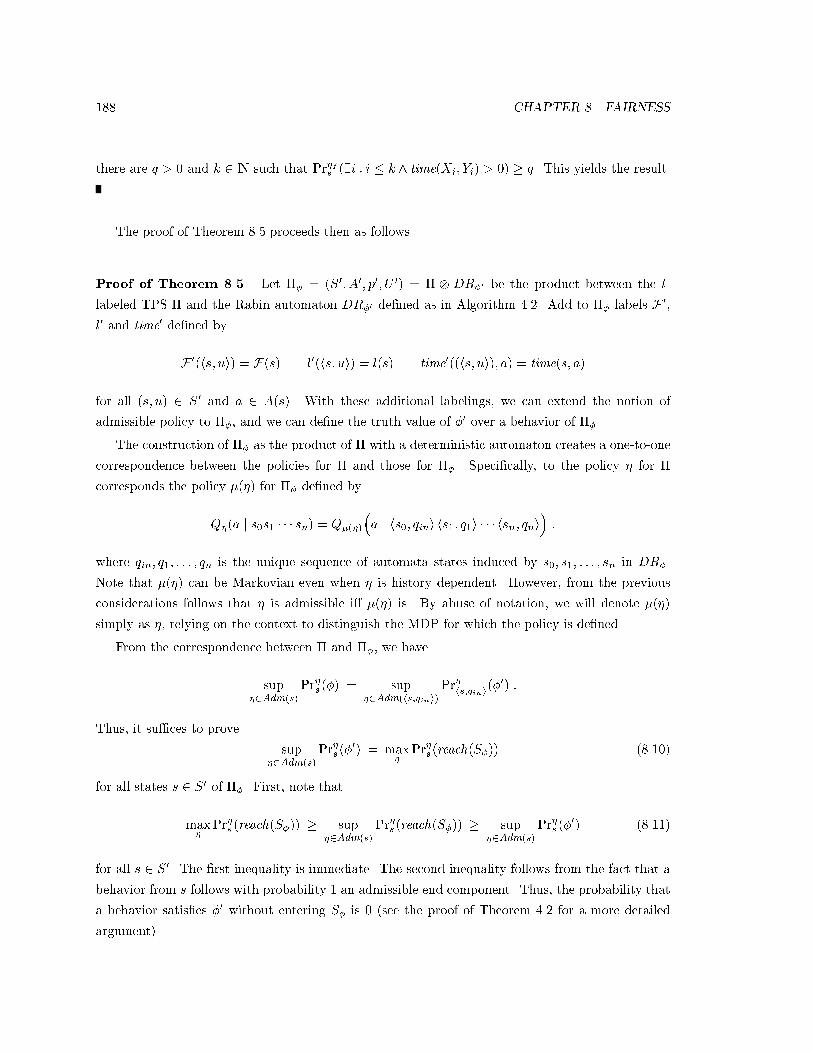
188 CHAPTER 8. FAIRNESS
there are q > 0 and k 2 IN such that Pr�fs (9i : i � k ^ time(Xi; Yi) > 0) � q. This yields the result.
The proof of Theorem 8.5 proceeds then as follows.
Proof of Theorem 8.5. Let �� = (S0; A0; p0; U 0) = � DR�0 be the product between the l-
labeled TPS � and the Rabin automaton DR�0 de�ned as in Algorithm 4.2. Add to �� labels F 0,
l0 and time0 de�ned by
F0(hs; ui) = F(s) l0(hs; ui) = l(s) time0((hs; ui); a) = time(s; a)
for all (s; u) 2 S0 and a 2 A(s). With these additional labelings, we can extend the notion of
admissible policy to ��, and we can de�ne the truth value of �0 over a behavior of ��.
The construction of �� as the product of � with a deterministic automaton creates a one-to-one
correspondence between the policies for � and those for ��. Speci�cally, to the policy � for �
corresponds the policy �(�) for �� de�ned by
Q�(a j s0s1 � � � sn) = Q�(�)
�a��� hs0; qini hs1; q1i � � � hsn; qni� ;
where qin; q1; : : : ; qn is the unique sequence of automata states induced by s0; s1; : : : ; sn in DR�.
Note that �(�) can be Markovian even when � is history dependent. However, from the previous
considerations follows that � is admissible i� �(�) is. By abuse of notation, we will denote �(�)
simply as �, relying on the context to distinguish the MDP for which the policy is de�ned.
From the correspondence between � and ��, we have
sup�2Adm(s)
Pr�s(�) = sup�2Adm(hs;qini)
Pr�hs;qini
(�0) :
Thus, it su�ces to prove
sup�2Adm(s)
Pr�s(�0) = max
�Pr�s(reach(S�)) (8.10)
for all states s 2 S0 of ��. First, note that
max�
Pr�s (reach(S�)) � sup�2Adm(s)
Pr�s(reach(S�)) � sup�2Adm(s)
Pr�s (�0) (8.11)
for all s 2 S0. The �rst inequality is immediate. The second inequality follows from the fact that a
behavior from s follows with probability 1 an admissible end component. Thus, the probability that
a behavior satis�es �0 without entering S� is 0 (see the proof of Theorem 4.2 for a more detailed
argument).

8.7. CORRECTNESS PROOF OF MODEL-CHECKING ALGORITHMS 189
In the reverse direction, let �m be a deterministic policy for �� such that
Pr�ms (reach(S�)) = max�
Pr�s (reach(S�)) : (8.12)
The existence of �m is guaranteed by Corollary 3.2. Let B � S0 be the set of states in S0 that cannot
reach S�. By (8.11), for s 2 B it is Pr�s (�0) = 0 under any policy �. From �m we can construct
a Markovian policy �M that di�ers from �m only on B and on S�. On S�, �M is constructed
as in the proof of Lemma 4.1; on B it coincides with �f . Since �m and �M coincide on the set
C = S0 � (B [ S�), it is
Pr�ms (reach(S�)) = Pr�Ms (�) (8.13)
for all s 2 C. Note also that �M is admissible. Given 0 � x � 1, denote by �(x) the Markovian
policy de�ned by
Q�(x)(a j s) =
((1� x)Q�M (a j s) + xQ�f (a j s) for s 2 C;
Q�M (a j s) for s 2 S� [B
for all s 2 S0 and a 2 A0(s), where �f is the admissible policy previously described.
For each 0 < x < 1, policy �(x) is admissible. In fact, outside of S� policy �(x) is fair, being
obtained by linear combination with �f , and time-divergent, for the same reason; inside S�, policy
�(x) coincides with �M .
Denote by P (x) = [pst(x)]s;t2C the transition matrix corresponding to policy �(x) restricted to
the set C of states. For 0 � x < 1, P (x) is a substochastic matrix. Note that P (0) is the transition
matrix for policy �M .
The closed recurrent classes of the Markov chain corresponding to P (x) are constant for 0 � x <
1. In fact, the closed recurrent classes of �M and �(x) are all contained in S� [B, and �M and �(x)
coincide on S� [ B. Denoting by P �(x) = [p�st(x)]s;t2C the steady-state matrix corresponding to
P (x), we can write the reachability probabilities as:
Pr�(x)s (reach(S�)) =Xt2S�
p�st(x) : (8.14)
From limx!0 P (x) = P�M , by Theorem 8.11 we have limx!0 P�(x) = P �
�M, and by (8.14) this yields
limx!0
Pr�(x)s (reach(S�)) = Pr�ms (reach(S�)) :
By (8.12) and (8.13), this indicates that
sup�2Adm(hs;qini)
Pr�hs;qini(�) � max�
Pr�hs;qini(reach(S�)) ;

190 CHAPTER 8. FAIRNESS
which is the other direction of (8.11). This completes the proof.
8.7.4 Model Checking D./a for ./2 f�; <g
To state the proofs, given a policy � we de�ne the vector w = [w�s ]s2S by
w�s = E�s
nT��1Xk=0
time(Xk; Yk)o
for all s 2 S. Thus, w�s represents the time needed to reach S� under �(x). For simplicity, we
consider in the following arguments a modi�ed TPS, in which every state s 2 S� has a single action
a, with time(s; a) = 1 and pss(a) = 1. This modi�cation does not change the expected time to S�,
which is the quantity that interests us. This modi�cation changes the set of admissible policies, but
it will not cause problems. In fact, in the original TPS once reached S� it is possible to follow policy
�f , ensuring admissibility. In the modi�ed TPS, once reached S� there is only one admissible policy
possible. The two conditions are equivalent for the purpose of our analysis.
Proof of Theorem 8.6. The proof follows the lines of the informal argument that precedes the
statement of the theorem, and is also related to the proof of Lemma 7.1.
Assume that there is an end component (C;D) 2 maxEC (S � S�) containing at least one state-
action pair (s; a) 2 sa(B;C) with time(s; a) > 0. Assume also that C is reachable from a state
s 2 S � S� without leaving S � S�. Then, the admissible policy �f of De�nition 8.11 will reach C
from s with positive probability. From �f , we de�ne another Markovian policy �m which coincides
with �f outside of C, and that at t 2 C chooses an action from D(s) uniformly at random.
If (C;D) is admissible, then �m is admissible, and from Pr�ms (T� = 1) > 0 we have
E�ms fPT��1k=0 time(Xk; Yk)g =1, from which follows the result.
If (C;D) is not admissible, for 0 � x < 1 we de�ne the policy �(x) by
Q�(x)(a j t) = (1� x)Q�m(a j t) + xQ�f (a j t)
for all t 2 S and a 2 A(t). Note that, for all 0 < x < 1, policy �(x) is admissible.
Let Pm be the transition matrix associated with �m, and P (x) be the matrix associated with
�(x), for 0 < x < 1. Note that limx!0 P (x) = Pm; however, for 0 < x < 1 the chain corresponding
to P (x) may have di�erent closed recurrent classes than the chain corresponding to P (0), so that
we cannot use the results about the continuity of the steady-state matrix. Instead, de�ne the vector
u = [us]s2S by
us =
8<:
1
2jD(s)j
Xa2D(s)
time(s; a) if s 2 C;
0 otherwise

8.7. CORRECTNESS PROOF OF MODEL-CHECKING ALGORITHMS 191
for all s 2 S. Note that at least one element of u is strictly positive.
Since u represents only part of the time spent along a behavior, for 0 < x < 1=2 we have
w�(x)s �
1Xk=0
P k(x)u :
In fact, when 0 < x < 1=2, at state s 2 C a behavior under �(x) will spend at least an expected
time of us with the next move: the limit 1=2 comes directly from the denominator in the de�nition
of us. For any �xed k it is limx!0 Pk(x) = P km, and since
P1k=0 P
kmu =1 it follows that
limx!0
1Xk=0
P (x)ku =1
from which we conclude limx!0 w�(x)s =1. The result then follows immediately.
Proof of Theorem 8.7. First, consider any admissible policy �; we want to prove that
Pr�s(reach(S�)) = 1 for all s 2 C. To see this, assume towards the contradiction that
Pr�s(reach(S�)) < 1. Then, there is an end component (B;D) with B � C such that Pr�s(inft(!) =
sa(B;D)) > 0. By de�nition of C, it must be time(t; a) = 0 for all (t; a) 2 sa(B;D). However, this
leads to
Pr�s
� 1Xk=0
time(Xk; Yk) <1
�> 0 ;
contradicting the admissibility of �.
Since Pr�s (reach(S�)) = 1, policy � is SSP-proper, and from the de�nition of the SSP problem
and the optimality of v� follows w� = �v� � �v�. From the arbitrariness of �, we have
sup�2Adm(s)
w�� �v
� (8.15)
for all s 2 C.
In the other direction, let �m be a Markovian SSP-proper policy optimal for the SSP problem,
i.e. such that v�m = v�. The existence of at least one such policy follows from the construction in
the proof of Theorem 7.1. There are two cases. If �m is admissible, then
w�m = �v
� : (8.16)
If �m is not admissible, for 0 � x < 1 de�ne the Markovian policy �(x) by
Q�(x)(a j s) = (1� x)Q�(a j s) + xQ�f (a j s)
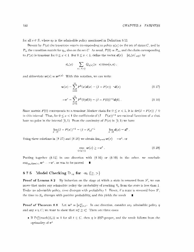
192 CHAPTER 8. FAIRNESS
for all s 2 S, where �f is the admissible policy mentioned in De�nition 8.11.
Denote by P (x) the transition matrix corresponding to policy �(x) on the set of states C, and by
Pm the transition matrix for �m also on the set C. As usual, P (0) = Pm, and the chain corresponding
to P (x) is transient for 0 � x < 1. For 0 � x < 1, de�ne the vector d(x) = [ds(x)]s2C by
ds(x) =X
a2A(s)
Q�(x)(a j s) time(s; a) ;
and abbreviate w(x) = w�(x). With this notation, we can write
w(x) =
1Xk=0
P k(x)d(x) = (I � P (x))�1d(x) (8.17)
�v� =
1Xk=0
P k(0)d(0) = (I � P (0))�1d(0) : (8.18)
Since matrix P (0) corresponds to a transient Markov chain for 0 � x < 1, it is det(I � P (x)) 6= 0
in this interval. Thus, for 0 � x < 1 the coe�cients of (I � P (x))�1 are rational functions of x that
have no poles in the interval [0; 1). From the continuity of P (x) in [0; 1) we have
limx!0
(I � P (x))�1 = (I � P�)�1 lim
x!0d(x) = d
� :
Using these relations in (8.17) and (8.18) we obtain limx!0w(x) = �v�, or
sup0<x<1
w(x) � �v� : (8.19)
Putting together (8.15) in one direction with (8.16) or (8.19) in the other, we conclude
sup�2Adm(s)w� = �v�, as was to be proved.
8.7.5 Model Checking D./a for ./2 f�; >g
Proof of Lemma 8.2. By induction on the stage at which a state is removed from S0, we can
prove that under any admissible policy the probability of reaching S� from the state is less than 1.
Under an admissible policy, time diverges with probability 1. Hence, if a state is removed from S0,
the time to S� diverges with positive probability, and this yields the result.
Proof of Theorem 8.8. Let w� = [w�s ]s2C . In one direction, consider any admissible policy �
and any s 2 C; we want to show that w�s � v�s . There are three cases.
� If Pr�t (reach(S�)) = 1 for all t 2 C, then � is SSP-proper, and the result follows from the
optimality of v�.

8.7. CORRECTNESS PROOF OF MODEL-CHECKING ALGORITHMS 193
� If Pr�s(reach(S�)) < 1, since the time diverges with probability 1 under � we have w�s = 1,
which leads to the result.
� If Pr�s(reach(S�)) = 1 and D = ft 2 C j Pr�t (reach(S�)) < 1g 6= ;, it is easy to see that there
is another policy �0, di�ering from � only at the states in D, such that �0 is SSP proper, and
w�0
t = w�t for all t 2 C �D. From w
�0 � v� follows w�s � v�s once more.
Since the result holds for any � and s 2 C, we conclude
inf�2�
A
w�� v
� : (8.20)
In the other direction, let �m be a Markovian SSP-proper policy optimal for the SSP problem,
i.e. such that v�m = v�. If �m is admissible, then w�m = v
�. Otherwise, we construct a family �(x)
of policies, with 0 � x < 1, such that limx!0w(x) = v�m = v
�. To construct the family, let �a be
a policy that, at s 2 C, chooses an action from A0(s) uniformly at random. From Algorithm 3.2, it
is easy to check that �a is admissible, and that Pr�as (reach(S�)) = 1 for all s 2 C. For 0 � x < 1,
de�ne
Q�(x)(a j s) = (1� x)Q�m(a j s) + xQ�a(a j s) :
Reasoning as in the proof of Theorem 8.7, we conclude
inf�2�
A
w�� v
� ;
which together with (8.20) yields the result.
8.7.6 Model Checking of Operators �P and �D
We state and prove the correctness of the model checking algorithm for �P and �D on fair TPSs with
the following theorem.
Theorem 8.13 (correctness model checking of �P and �D on fair TPSs) The modi�cations
presented in Section 8.5.7 to the algorithm of Section 6.1.2 yield a correct algorithm for the model
checking of the operators �P and �D on fair TPSs.
Proof. The �rst step in proving the result consists in showing the correctness of the decomposition
into maximal admissible end components of Step 1', as opposed to the decomposition in maximal
end components of Step 1. This is justi�ed by Theorem 8.3, which states that under an admissible
policy, behaviors eventually follow an admissible end component with probability 1. A formal proof
can be done by repeating the argument of Theorem 6.4 in the context of fair MDPs.
Next, consider a sub-MDP �i = (Si; Ai; pi; Ri;Wi) 2 L, and assume that ./2 f�; >g; the case
for ./2 f�; <g is similar. If i 2 K�
, let J0 = ��i ; otherwise, let J0 = �1. We have to show that, for

194 CHAPTER 8. FAIRNESS
all s 2 Si, it is �FT�s = J0. To prove this result, it su�ces to show that the following two assertions
hold:
1. For any admissible policy � for �i, and any s 2 Si, it is
Pr�s
�lim infn!1
Hn(!) < J0
�= 0 : (8.21)
2. For any s 2 Si, it is
J0 � inf�2Adm(s)
nJ��� Pr�s�lim inf
n!1Hn(!) = J
�= 1o: (8.22)
Assertion 1 follows immediately from the results of Chapter 6, since the set of admissible policies
is a subset of the set of all policies. To prove Assertion 2, we proceed as follows. By Corollary 6.7,
there is an unichain policy �m such that
Pr�ms
�limn!1
Hn(!) = J0
�= 1 :
If �m is admissible, we are done. Otherwise, denote by C � Si the single closed recurrent class of
�m. Let �f be the admissible Markovian policy which at every state s 2 Si chooses an action from
Ai(s) uniformly at random, and for 0 � x < 1, de�ne the Markovian policy �(x) by
Q�(x)(a j s) = (1� x)Q�m(a j s) + xQ�f (a j s) ;
for all s 2 Si and a 2 Ai(s). From this de�nition, we see that policy �(x) is admissible for all
0 < x < 1. Let P (x) be the matrix of the Markov chain corresponding to �(x), and de�ne the
vectors R(x) = [Rs(x)]s2Si and W (x) = [Ws(x)]s2Si by
Rs(x) =X
a2Ai(s)
Ri(s; a)Q�(x)(a j s) Ws(x) =X
a2Ai(s)
Wi(s; a)Q�(x)(a j s) ;
for all s 2 Si.
Note that the policy �(x) is unichain for all 0 � x < 1: its closed recurrent class is equal to C
for x = 0, and to Si for 0 < x < 1. Pick an arbitrary state s0 2 C: state s0 is thus surely recurrent
for all 0 � x < 1. Hence, we can apply Theorem 8.12, obtaining as a result the continuity of �(x)
for all 0 � x < 1. The result (8.22) then follows from
limx!0
�(x)R(x)
�(x)W (x)= J0

8.7. CORRECTNESS PROOF OF MODEL-CHECKING ALGORITHMS 195
and from
Pr�(x)s
�limn!1
Hn(!) =�(x)R(x)
�(x)W (x)
�= 1 :
The proof is completed by combining Assertions 1 and 2.

Chapter 9
Veri�cation of Stochastic
Transition Systems
The previous chapter concluded our presentation of temporal logics and model-checking algorithms
for TPSs. Armed with these results, we return to the speci�cation and veri�cation of stochastic
transition systems (STSs), which has been informally described in Chapter 2.
The �rst step in this direction consists in de�ning a formal semantics for STSs. We de�ne this
semantics by means of a translation from STSs to fair TPSs. This translation is also used for the
veri�cation of STSs, since our model-checking algorithms can be applied to fair TPSs, rather than
STSs. This translation is faithful to the informal semantics presented in Section 2.1.2: this result
is of practical interest, since usually the model of a real system is constructed with that informal
semantics in mind, rather than with the formal semantics de�ned by translation.
An alternative approach, not followed here, consists in formalizing the informal semantics of
Section 2.1.2, taking that de�nition as basic. If we followed this approach, we would have to prove
the correspondence between the formal semantics of STSs and the semantics of their translations into
fair TPSs. Since in this dissertation we place the emphasis on logics and model-checking algorithms,
rather than semantical arguments, we prefer to avoid this additional step. We rely instead on a
precise but informal argument to justify our translation.
The speci�cation of probabilistic properties of STSs relies on the logics SPTL and SPTL*. These
logics di�er from FPTL and FPTL* only for a minor change in the semantics. The change has been
introduced to account for the characteristics of the translation process, which introduces auxiliary
states that have no counterpart in the original STS. The model-checking algorithms described in
the previous chapter can be used with minor adaptations to decide whether an STS satis�es speci-
�cations written in these new logics. We conclude the chapter with some remarks about the role of
nondeterminism in STSs.
196

9.1. TRANSLATION OF STSS INTO TPSS 197
9.1 Translation of STSs into TPSs
The translation from STSs to fair TPSs is based on the informal semantics for STSs presented in
Section 2.1.2. Given an STS S = (V ;�; T ), its translation �S = (S [ bS;A; p;F ; bS; Sin; time; I) isa translation TPS, formed by a fair TPS (S [ bS;A; P;F ; Sin; time; I) together with a distinguished
subset bS of auxiliary states. We de�ne the translation TPS �S by stages.
Principal states. As in De�nition 2.1, the set V of typed variables of the STS gives rise to a
set S of states consisting of all type-consistent interpretations of the variables in V . Since in this
dissertation we are discussing only the veri�cation of �nite-state systems, we assume that all the
variables in V have �nite domain, so that S is a �nite set. We call S the set of principal states of �S .
In addition to S, the translation will introduce also the set bS of auxiliary states. For each s 2 S, we
let Is[[x]] = s[[x]].
The set Sin of initial states is de�ned simply as Sin = fs 2 S j s j= �g, and consists thus of
principal states only.
9.1.1 Transition Structure of Principal States
Let T (s) = f� 2 T j s j= E�g be the set of STS transitions enabled at a principal state s 2 S. In
analogy with the de�nition of informal semantics of STS of Section 2.1.2, the transition structure
associated with s depends on whether T (s) contains immediate transitions or not.
Some Immediate Action Enabled
Let Ti(s) = T (s) \ Ti be the set of immediate transitions enabled at s, and assume that Ti(s) 6= ;.
In this case, we let A(s) = fa� j � 2 Ti(s)g, where action a� represents the choice of transition �
at s. For all � 2 Ti(s), we let time(s; a� ) = 0; moreover, action a� is fair at s i� � is fair: formally,
a� 2 F(s) i� � 2 Tf , for all � 2 Ti(s).
For each � 2 Ti(s), we add to bS the auxiliary states (s; h�; ji), where 1 � j � m� . Each auxiliary
state (s; h�; ji) represents the choice of mode j of transition � from state s. Since auxiliary states
represent choices done while at a principal state, we let I(s;h�;ji)[[x]] = s[[x]], for � 2 Ti(s) and
1 � j � m� .
For � 2 Ti(s) and 1 � j � m� , the transition probability from s to (s; h�; ji) is de�ned by
ps;(s;h�;ji)(a� ) = p�j ;
where p�j is the probability of mode j of transition � . All other transition probabilities are 0.

198 CHAPTER 9. VERIFICATION OF STOCHASTIC TRANSITION SYSTEMS
No Immediate Transitions Enabled
If T (s) � Td, we let
Te(s) = T (s) \ Te Tu(s) = T (s) \ Tu ;
note that Te(s) 6= ;, due to the presence of the idling transition. We let
A(s) = faeg [ fa� j � 2 Tu(s)g ; (9.1)
action ae represents the choice of a transition with exponential distribution, while action a� repre-
sents the choice of the transition � , with unspeci�ed delay distribution.
We let F(s) = A(s), and we de�ne the expected times of the actions by
time(s; ae) =
� X� 02Te(s)
� 0
��1time(s; a� ) = 0 (9.2)
for all � 2 Te(s). These decisions will be justi�ed once the presentation of the translation is com-
pleted.
For each � 2 T (s), we add to bS the auxiliary states (s; h�; ji), where 1 � j � m� . Each auxiliary
state (s; h�; ji) represents the choice of mode j of transition � from state s. Since auxiliary states
represent choices done while at a principal state, we let I(s;h�;ji)[[x]] = s[[x]], for � 2 T (s) and
1 � j � m� .
The transition probabilities to these auxiliary states are de�ned as follows. For � 2 T (s) and
1 � j � m� , we let
� 2 Tu(s) : ps;(s;h�;ji)(a� ) = p�j (9.3)
� 2 Te(s) : ps;(s;h�;ji)(ae) = p�j �
� � X� 02Te(s)
� 0
�; (9.4)
where p�j is the probability of mode j of transition � . All other transition probabilities are 0.
9.1.2 Transition Structure of Auxiliary States
Consider an arbitrary auxiliary state (s; h�; ji) 2 bS. This state represents the choice of mode j of
action � at principal state s. Let T �j (s) = fs0 2 S j (s; s0) j= ��j g be the set of possible successor
states of s according to this transition mode. We let A(s; h�; ji) = T �j (s), and
p(s;h�;ji);t(t) = 1 time(s; t) = 0

9.1. TRANSLATION OF STSS INTO TPSS 199
for all t 2 T �j (s), with all other transition probabilities from the auxiliary state being 0. None of the
actions from the auxiliary state is fair: we set F(s; h�; ji) = ;.
The presentation of the translation from STSs to fair TPSs is thus concluded.
9.1.3 Complexity of Translation and Optimizations
The following theorem relates the size of an STS to the size of its translation TPS.
Theorem 9.1 (size of translation TPS) Given an STS S = (V ;�; T ), let �S be the translation
TPS for S. Denote by S the set of states arising from the set of variables V, and letM = max�2T m� .
The size j�S j is then polynomial in M � jSj � jT j.
Proof. The result follows immediately from an exam of the translation process.
To reduce the size of the translation TPS, it is possible to eliminate the idling transition from
the set T (s) of transitions enabled at a state s, provided the set T (s) does not become empty. We
have retained the idling transition in our de�nition of translation purely to simplify the de�nition.
Another optimization consists in avoiding the generation of auxiliary states that have only one
successor state. More precisely, assume that for state s 2 S, transition � 2 T (s) and mode 1 � j �
m� there is only one state t 2 S such that (s; t) j= ��j . In this case, instead of creating the auxiliary
state (s; h�; ji) having t as single successor, we can direct all transitions to this auxiliary state to the
principal state t instead. This optimization succeeds in removing all auxiliary states corresponding
to deterministic transitions.
9.1.4 An Example of Translation
Consider the TPS S = (V ;�; T ) with set of variables V = fxg, initial condition � : x = 0 and set
of transitions T = f�1; �2; �3; �4g. The domain of x is f0; 1; 2; 3g, and the transitions are as follows:
� Transition �1 2 Te has rate �1 = 2 and m�1 = 1. Its enabling transition and transition formula
are, respectively, E�1 : x < 3 and ��1 : x0 = x+ 1.
� Transition �2 2 Te has rate �2 = 1 and m�2 = 1. Its enabling transition and transition formula
are, respectively, E�2 : x > 0 and ��2 : x0 = x� 1.
� Transition �3 2 Ti is immediate, and it is m�3 = 1. Its enabling transition and transition
formula are, respectively, E�3 : x = 0 and ��3 : x0 = 1 _ x0 = 2.
� Transition �4 2 Tu has unspeci�ed rate, and it ism�4 = 1. Its enabling transition and transition
formula are, respectively, E�4 : x = 3 and ��4 : x0 = 0.

200 CHAPTER 9. VERIFICATION OF STOCHASTIC TRANSITION SYSTEMS
0
1/3 2/3
2/31/3
1
23
aaτ2 τ4
Figure 9.1: Translation TPS �S . The principal states are depicted as �lled circles, and are labeledwith the corresponding value of x. The names of the auxiliary states have been omitted, and onlythe names of some actions have been indicated. The auxiliary states denoted by a dot have onlyone successor state, and can be eliminated by a simple optimization.
This STS represents a continuous-time random walk between the integers 0, 1, 2, and 3. If x < 3,
there is an exponential transition with rate 2 that increases x; if x > 0 there is an exponential
transition with rate 1 that decreases x. The random walk has boundaries 0 and 3. When boundary 0
is reached, there is an instantaneous transition that sets x to either 1 or 2. When boundary 3
is reached, alongside the transition with exponential distribution that decreases x is activated a
transition with unspeci�ed rate that sets x to 0.
The translation TPS � is depicted in Figure 9.1. To reduce clutter, we have used the optimiza-
tion of omitting the idling transition, since there is at least one transition enabled on every state.
Denote by si the principal state where x = i, for 0 � i � 3. The expected times of the actions from
s3 are given by time(s3; a�2) = 1 and time(s3; a�4) = 0. The only action from state s0 has expected
time 0. The only actions from states s1 and s2 have expected times 1/3. The expected times of
actions from auxiliary states are always 0, by our de�nition of translation. In Figure 9.2 we depict
the translation TPS obtained from the one of Figure 9.1 by applying the optimization of removing
all auxiliary states having only one successor.
9.2 Translation and Informal Semantics
Even though the formal semantics of STSs is de�ned by translation into fair TPSs, there is a corre-
spondence between the proposed translation and the informal semantics presented in Section 2.1.2.

9.2. TRANSLATION AND INFORMAL SEMANTICS 201
aτ2
aτ4
0
2/31/3
1
23
2/31/3
Figure 9.2: Result of removing all auxiliary states having only one successor from the TPS ofFigure 9.1.
This correspondence is important from a pragmatic point of view, since the models of real probabilis-
tic systems are usually constructed in terms of this intuitive semantics. We justify the translation
in three steps, considering �rst the structure of the translation TPS, then the use of fairness, and
lastly the interaction between translation and speci�cation languages.
9.2.1 Structure of the Translation TPS
To understand the correspondence between the translation and the informal semantics, consider
�rst auxiliary states. As remarked in the de�nition of translation, auxiliary states represent a
choice of transition and transition mode from a principal state. The introduction of these states is
necessary because of the di�erent interaction between probability and nondeterminism in Markov
decision processes and STSs. In a Markov decision process, the successor of a state is chosen
in two steps, a nondeterministic one (the choice of action) and a probabilistic one (the choice of
destination state). In an STS, there are up to three steps: the choice of transition (probabilistic or
nondeterministic), the choice of transition mode (probabilistic), and �nally the choice of destination
state (nondeterministic). The role of auxiliary states is precisely to accommodate the three-step
selection process of STSs into the two-step one of TPSs.
Consider now the system evolution from a principal state s. If there are immediate transitions
enabled at s, the correspondence between the informal semantics of the STS and the translation
TPS is immediate.
If the set T (s) of transitions enabled at s is a subset of the delayed transitions Td, let as before
Te(s) = T (s)\Te and Tu(s) = T (s)\Tu. When a behavior of the TPS reaches s, the set of available
actions is faeg[fa� j � 2 Tu(s)g. Let qe and q� , for � 2 Tu(s), be the probabilities with which these
actions are chosen by a policy. Note that these probabilities can depend on the past history of the
TPS.
There is a relation between the probabilities qe and q� , � 2 Tu, selected by the policy, and the

202 CHAPTER 9. VERIFICATION OF STOCHASTIC TRANSITION SYSTEMS
rates of the transitions in Tu(s), selected nondeterministically in the informal semantics. To derive
the relation, consider the probability of choosing � 2 T (s) in the TPS and in the informal semantics.
From (9.3) and (9.4), the probability of choosing � 2 T (s) in the TPS is given by
� 2 Te(s) : qe �
�� X� 02Te(s)
� 0
�(9.5)
� 2 Tu(s) : q� : (9.6)
In the informal semantics, the probability is given by
�
� � X� 02T (s)
� 0
�(9.7)
for all � 2 T (s), which is just a restatement of (2.2). Equating (9.7) with (9.5) and (9.6), we obtain
qe =
� X� 02Te(s)
� 0
� � � X� 02T (s)
� 0
�q� = �
� � X� 02T (s)
� 0
�(9.8)
for all � 2 Tu(s).
This relation between qe, fq�g�2Tu(s) and f �g�2Tu(s) preserves not only the probabilities of
choosing the transitions at s, but also the expected time spent at s. In fact, from (9.2) the expected
time spent by the TPS at s is given by
qe
�� X� 02Te(s)
� 0
�: (9.9)
If we substitute into this equation the value of qe given by (9.8), we obtain
X� 02Te(s)
� 0
� X� 02T (s)
� 0
�� X� 02Te(s)
� 0
� =
� X� 02T (s)
� 0
��1;
which is exactly the expected time spent at s under the informal STS semantics, as de�ned by (2.1).
Thus, equations (9.8) together with the constraint qe +P�2Tu(s)
q� = 1 de�ne a one-to-one
mapping between the unspeci�ed transition rates in the informal STS semantics and the probabilities
of choosing the actions in the translation TPS. The mapping preserves both the expected time spent
at s, and the probabilities of selecting transitions from s. Given a nondeterministic choice for the
transition rates f �g�2Tu(s), we can determine a policy which simulates this choice; conversely, each
policy can be interpreted as a choice for these rates. This correspondence indicates that the proposed
translation of STS into fair TPS preserves the informal semantics presented in Section 2.1.2.

9.2. TRANSLATION AND INFORMAL SEMANTICS 203
τ(s,< ,1>)2
(s,< ,1>)τ1
ae
τa2
γ1-1
t 1
t 2
0
00
s
Figure 9.3: Portion of translation TPS corresponding to states s; t1; t2 and transitions �1; �2. Eachedge is labeled by the expected time corresponding to the source state and the action.
9.2.2 Translation and Fairness
The above considerations also justify our use of fairness in the translation, and more generally our
de�nition of probabilistic fairness.
In fact, for � 2 Tu(s) the fairness of a� requires that q� > 0, which by (9.8) corresponds to the
requirement � > 0. Similarly, the fairness of ae requires that qe > 0, which corresponds to the
requirement � < 1 for all � 2 Tu(s). Thus, the fairness requirements associated with principal
states in the translation TPS are the exact counterpart of the requirements 0 < � < 1 for the
rates of transitions � 2 Tu.
From this we see that fairness gives us precisely the tool needed to represent transitions with
unspeci�ed delay distributions in our translation TPS. This consideration has been one of the main
motivations for our new de�nition of probabilistic fairness.
9.2.3 Translation and Speci�cation Language
We conclude our justi�cation of the translation with a remark about the relationship between the
translation and the speci�cation languages presented in this dissertation.
In (9.2), we assign an expected time 0 to the actions that correspond to transitions with unspeci-
�ed rates. This assignment is justi�ed by our previous considerations on the equivalence of choosing
the transition rates in the STS, and choosing the policy in the TPS. However, the justi�cation is
incomplete without the observation that the speci�cation languages we presented can only refer to
the expected time spent at a state, not conditional on the successor state.
To clarify this point, consider a state s on which two transitions are enabled: a transition �1,
with rate 1, and a transition �2, with unspeci�ed rate. The two transitions have only one mode, and
they lead to states t1 and t2, respectively. The portion of translation TPS for s, �1, �2 is depicted
in Figure 9.3. The translation would be inappropriate if our speci�cation languages could express

204 CHAPTER 9. VERIFICATION OF STOCHASTIC TRANSITION SYSTEMS
properties such as:
the time spent at s when (s; h�2; 1i) is the immediate successor is on average > b.
In fact, for the purposes of this property the choice of assigning time(s; a�2) = 0 would not correspond
to the idea of assigning nondeterministically a transition rate to �2.
However, an exam of the semantical de�nitions of our speci�cation languages reveals that the
languages cannot specify properties in which the expected time is measured conditionally on the
successor state. The key de�nitions are de�nition (4.15) and (8.1) of semantics of D, and De�nitions
5.5 and 8.6 of product between TPS and D-experiment.
� In (4.15) and (8.1), for any k � 0, the fact that the time time(Xk; Yk) belongs to the summation
depends only on the sequence of states X0 � � �Xk, and not on the successor state Xk+1.
� In De�nitions 5.5 and 8.6, consider a state hs; ui of the product MDP. If u is a timed vertex,
all actions from hs; ui contribute to r; if u is untimed, none of the actions does. Hence, the
contribute of the r label does not depend on the successor state of hs; ui.
These observations conclude our justi�cation of the translation process.
9.3 Speci�cation and Veri�cation of Stochastic Transition
Systems
For the speci�cation of probabilistic properties of STSs, we introduce the new logics SPTL and
SPTL*. The di�erence between these logics and the fair probabilistic logics FPTL and FPTL* is
limited to the semantics of state formulas, and is motivated by the presence of auxiliary states in
the translation TPS. The de�nition is as follows.
De�nition 9.1 (semantics of SPTL, SPTL* formulas) Let � = (S [ bS, A, p, F , Sin, time,I, bS) be a translation TPS, where bS is the set of auxiliary states, and consider a state formula � of
SPTL or SPTL*.
The truth value of � at a principal state s 2 S � bS is de�ned using the same clauses of FPTL
and FPTL*. The truth value of � at an auxiliary state (s; h�; ji) 2 bS is de�ned by
(s; h�; ji) j= � i� s j= � : (9.10)
Thus, the truth value of a state formula at an auxiliary state is equal to the truth value of the same
state formula at the corresponding principal state.
We say that an STS satis�es a speci�cation i� its translation TPS does.

9.3. SPECIFICATION AND VERIFICATION OF STOCHASTIC TRANSITION SYSTEMS 205
De�nition 9.2 (satisfaction of speci�cation over STS) Consider an STS S = (V ;�; T ) and
its translation TPS �S = (S [ bS;A; P;F ; Sin; time; I; bS). Given a speci�cation � 2 Stat of SPTL or
SPTL*, we say that �S j= � i� s j= � for every s 2 Sin, and we say that S j= � i� �S j= �.
To understand the rationale for De�nition 9.1, note that under the semantics for FPTL and
FPTL* it is possible for a state formula to assume di�erent truth values on a principal state and on
the related auxiliary states. For example, the expected time to reach a given set of states can be
di�erent when measured from a principal state, or from an auxiliary state where the next transition
has already been selected. If our de�nition of semantics took into account the truth values of
state formulas at auxiliary states, the logic would present often counterintuitive and undesirable
properties. The following example illustrates this situation.
Example 9.1 Consider an STS S = (V ;�; T ), where:
� V = fxg, and the domain of x is f0; 1g;
� � : x = 0;
� T = Te = f�0g, where the exponential-delay transition �0 is de�ned by enabling condition
E�0 : true, transition rate �0 = 1, number of modes m�0 = 1, and transition relation �0 : x0 =
1� x.
Informally, the STS S describes a system that oscillates between states 0 and 1, and whose switch-
ing time from one state to the other obeys an exponential distribution with unit rate. Since
the exponential distribution is memoryless, if the system is in state 0, the expected amount
of time needed to reach state 1 is 1. Thus, we expect S to satisfy the FPTL speci�cation
�0 : A2[x = 0! D�0:7(x = 1)].
However, consider the translation TPS �S depicted in Figure 9.4. To understand its structure,
recall that to any STS is implicitly added the idling transition �idle. From state s0, the expected
time to a state where x = 1 is 1, so that D�0:7(x = 1) holds at s0. However, the expected time
to x = 1 from state (s0; h�0; 1i) is 0, since the only action from this auxiliary state leads to s1 and
has expected time 0. This implies that D�0:5(x = 1) does not hold at (s0; h�0; 1i) under the normal
de�nition of semantics, leading to S 6j= �0.
This example demonstrates that the truth value of state formulas at auxiliary states is not
necessarily related to any property of the physical system being modeled. In this very simple
example, the problem is eliminated if we apply the optimization of removing the auxiliary states
having only one successor, but this of course is no solution in general. If our de�nition of semantics
took into account these truth values, our logics would have scarce use as speci�cation languages.
Under the semantics provided by De�nition 9.1, the truth values of state formulas at auxiliary states
are disregarded, and we have S j= �0 as expected.

206 CHAPTER 9. VERIFICATION OF STOCHASTIC TRANSITION SYSTEMS
s0ae
aes1
s1 τidle( ,< ,1>)
s1 τ0
s0( ,< ,1>)τ0
s0 τidle( ,< ,1>)
( ,< ,1>)
1/2
1/2
1/2
1/2
Figure 9.4: Translation TPS �S obtained from the STS described in Example 9.1. The principalstates are s0, s1, and are depicted as �lled circles; the other states are auxiliary states. Variablex assumes value 0 at s0 and at the two auxiliary corresponding to s0, and value 1 at the otherstates; the initial state is s0. It is time(s0; ae) = time(s1; ae) = 1=2; the expected times of the otherstate-action pairs are 0.
Veri�cation of Stochastic Transition Systems
Due to the similarity between the semantics of SPTL, SPTL* and FPTL, FPTL*, the algorithms that
have been presented in the previous chapter for the model checking of FPTL, FPTL* speci�cations
can be immediately adapted to SPTL and SPTL*.
To decide the truth value of a speci�cation � 2 Stat at all initial states of a translation TPS �S ,
we recursively evaluate the truth values of the state subformulas of � at all states, until the truth
value of � itself can be computed at all initial states. With respect to the algorithms for FPTL and
FPTL*, the only change consists in the fact that the truth value of state formulas at auxiliary states
is de�ned by (9.10), rather than being computed directly. This modi�cation does not change the
complexity of the model-checking algorithms, which share the same complexity bounds of those for
FPTL and FPTL*.
9.4 A Highway Commuter Example
Having concluded the presentation of our methodology for formal speci�cation and veri�cation of
systems, we present a �nal example. Our system, highway-repair, is shown in Figure 9.5, and
models a commuter that travels perennially back and forth between two cities A and B, passing
through an intermediate city C.

9.4. A HIGHWAY COMMUTER EXAMPLE 207
city A
Possiblecommuterstates
highway segment 1 highway segment 2
city C
city B
1 2
34
(c)
Figure 9.5: System highway-repair. Depicted are also the 4 possible states of the commuter,represented by the values 1..4 of variable c.
Each of the two highway segment from A to C and from C to B can be in one of three states: good ,
broken and repair , modeling a good stretch of highway, one with pot-holes in it, and one under repair.
For a highway segment, the transition from good to broken has rate gb, and the transition from
repair to good has rate rg . The transition from state broken to state repair, instead, has unspeci�ed
delay distribution: the criteria with which the organizations in charge of road maintenance decide
to start repair works are not known to the layperson.
As depicted in Figure 9.5, the commuter can be at one of 4 states, depending on which segment
must be traversed next, and in which direction. Depending on the state in which the next link is,
the commuter traverses the link with rate g, b or r.
The STS � = (V ;�; T ) for this example has set of variables V = fl1; l2; cg, where l1 and l2
have domain fgood; broken; repairg and represents the link status, and c has domain f1; 2; 3; 4g and
represents the position of the commuter. The initial condition is � : true. Note that the initial
condition is not important, since we are interested in the steady-state behavior of the system, which
does not depend on the initial condition, as all states are reachable from all other states.
The transitions are divided in two groups: the transitions that describe the status of the highway
links, and the transitions that describe the commuter. All of these transitions have only one mode,
so that for every � 2 T it is m� = 1 and p�1 = 1. To avoid clutter, when describing transition � we
write E instead of E�1 , and similarly for the other components.
Highway link transitions. The transitions for the highway links are as follows, for i = 1; 2.
� Transition � igb 2 Td has rate gb, and it has E : li = good and � : l0i = broken.
� Transition � ibr 2 Tu has E : li = broken and � : l0i = repair.
� Transition � irg 2 Td has rate rg, and it has E : li = repair and � : l0i = good.

208 CHAPTER 9. VERIFICATION OF STOCHASTIC TRANSITION SYSTEMS
Ψ1/2Ψ1
c=1 c=1 c=1 c=2 c=3 c=4
Figure 9.6: Experiments for the speci�cation of one-way trip and round-trip commuter times insystem highway-repair. Experiment 1 measures the round-trip time, experiment 1=2 the one-way trip time from A to B. All edges of the two experiments are timed, and thus shown in boldface.
Commuter transitions. There are three transitions for the commuter, depending on the condi-
tion of the link to be traversed.
� Transition �cg 2 Td has rate g, and it has
E : [(c = 1 _ c = 4) ^ l1 = good ] _ [(c = 2 _ c = 3) ^ l2 = good ] c0 = (c mod 4) + 1 :
� Transition �cr 2 Td has rate r, and it has
E : [(c = 1 _ c = 4) ^ l1 = repair ] _ [(c = 2 _ c = 3) ^ l2 = repair ] c0 = (c mod 4) + 1 :
� Transition �cb 2 Td has rate b, and it has
E : [(c = 1_ c = 4)^ l1 = broken ]_ [(c = 2_ c = 3)^ l2 = broken ] c0 = (c mod 4)+1 :
The set of transitions of the STS is thus
T =n�1gb; �
1br; �
1rg; �
2gb; �
2br ; �
2rg; �
cg ; �
cb ; �
cr
o:
The TPS resulting from this STS, after the simple optimizations, consists of 32 � 4 = 36 states.
The speci�cations we write for this TPS refer to the average time required for the commuter to go
from A to B, and for the commuter to perform a round-trip. These speci�cations are written with
the help of the experiments depicted in Figure 9.6. The two speci�cations we write are:
�D�14(1) �D�7(1=2) :
These speci�cations require that the time required for a round-trip (resp. halftrip) is on average less
than 14 (resp. 7).

9.5. CONCLUDING REMARKS 209
Consider the case in which the transition rates are given by:
gb = 0:05 rg = 0:1 g = 0:5 r = 0:3 b = 0:1 :
Using the model-checking algorithms presented in the dissertation, it can be decided that all states
s of � are such that
s j= �D�14(1) s 6j= �D�7(1=2) :
Thus, the long-run average duration of a round-trip is guaranteed to be at most 14 time units, but
the long-run average duration of a one-way trip is not guaranteed to be at most 7 time units! The
model-checking algorithm enables to establish that, approximately, the threshold outcomes are
�FT�s (1) ' 11:7774 �FT
�s (1=2) ' 5:5458
�FT+s (1) ' 13:5986 �FT
+s (1=2) ' 7:5526
for all states s of �. Intuitively, this can be explained as follows. The policy �1 that maximizes
the round-trip time of the commuter tries to slow down the commuter along the entire round-trip,
without discriminating the �rst from the second part of the round-trip. On the other hand, the
policy �1=2 that maximizes the one-way time concentrates the slowdown on the �rst part, from city
A to B, without making slowdown e�orts during the return part of the trip. Since the slowdown in
this latter case is concentrated on the part of trip that is being monitored by the experiment, the
time required to complete it will be on average more than half of the time required to complete a
round-trip.
9.5 Concluding Remarks
We would like to conclude this presentation with some remarks on the use of nondeterminism in the
modeling and speci�cation of probabilistic systems. We take as starting points the highway-repair
system, and the example of the token ring system presented in Chapter 2.
Nondeterminism can have di�erent functions in a system model. For example, it can be used to
model unknown schedulers, and unspeci�ed \black-box" algorithms that can be implemented. This
was the case in the token-ring example, where we used nondeterminism to model the leader-election
algorithm and the recoveries from failure. Another use of nondeterminism, as we have seen in this
chapter, is to represent transitions having unknown distributions of waiting times.
Regarding this last use of nondeterminism, it is important to realize that nondeterminism not only
implies that the waiting-time distribution of the system is unspeci�ed, but also that the distribution
might in fact depend on the past history of the system, or on the current state of the system |
including portions of the state that might not seem at �rst related to the transition. For example,

210 CHAPTER 9. VERIFICATION OF STOCHASTIC TRANSITION SYSTEMS
in the last system we modeled the highway-segment transition from broken to repair by a transition
with unspeci�ed distribution. This implies that the organization in charge of highway maintenance
can decide how to schedule the repair works as a function of the system state (our results from
Chapter 6, together with the forms of experiments 1 and 1=2, imply that the pessimal strategies
need not depend on the past).
It seems quite reasonable to allow the repair policy to depend on the state of the links: this
makes it possible to model facts such as a preference, on the organization's part, for repairing at
most one segment at a time. On the other hand, it seems at �rst rather unreasonable to enable the
policy to depend on where the commuter is. It is as if the repair organization, to decide whether
to begin repair works, looks at where a speci�c unlucky commuter is! Of course, many people feel
that this is exactly what must be happening to them when they travel. Beyond this pessimistic
explanation, however, there is a more complicated picture.
It might indeed be unreasonable to expect that the repair policy is based on the position of
a single unlucky commuter. However, it is possible that there are external events that in uence
both the commuter and the repair policy. For example, the commuter might start the journey from
city A to B always in the mornings, and the organization might also prefer to start repair work in
the mornings.
As these considerations demonstrate, the use of nondeterminism in the construction of a system
model is a complex issue. In this dissertation, we have taken the approach of granting the highest
possible degree of freedom to nondeterminism: nondeterministic choices can be randomized, and
can depend on the full history of the system. This approach guarantees that system models are a
conservative approximation of real systems: if a system model can be shown to satisfy a speci�cation,
the real system will also satisfy it. It would be very interesting, nonetheless, to examine intermediate
concepts of nondeterminism, in which the policy is not known in advance, but not completely
unconstrained either.

Bibliography
[ABC84] M. Ajmone Marsan, G. Balbo, and G. Conte. A class of generalized stochastic Petri
nets for the performance analysis of multiprocessor systems. ACM Trans. Comp. Sys.,
2(2):93{122, May 1984.
[ABC+94] M. Ajmone Marsan, G. Balbo, G. Conte, S. Donatelli, and G. Franceschinis. Modelling
with Genralized Stochastic Petri Nets. John Wiley & Sons, 1994.
[ACD90] R. Alur, C. Courcoubetis, and D. Dill. Model-checking for real-time systems. In Proc.
5th IEEE Symp. Logic in Comp. Sci., 1990.
[ACD91] R. Alur, C. Courcoubetis, and D.L. Dill. Model-checking for probabilistic real-time
systems. In Proc. 18th Int. Colloq. Aut. Lang. Prog., volume 510 of Lect. Notes in
Comp. Sci., pages 115{126. Springer-Verlag, 1991.
[ACD92] R. Alur, C. Courcoubetis, and D. Dill. Verifying automata speci�cations of probabilistic
real-time systems. In Real Time: Theory in Practice, volume 600 of Lect. Notes in
Comp. Sci., pages 28{44. Springer-Verlag, 1992.
[AD90] R. Alur and D. Dill. Automata for modeling real-time systems. In Proc. 17th Int. Colloq.
Aut. Lang. Prog., volume 443 of Lect. Notes in Comp. Sci., pages 322{335. Springer-
Verlag, 1990.
[AFK88] K.R. Apt, N. Francez, and S. Katz. Appraising fairness in languages for distributed
programming. Distributed Computing, 2:226{241, 1988.
[ASB+95] A. Aziz, V. Singhal, F. Balarin, R.K. Brayton, and A.L. Sangiovanni-Vincentelli. It
usually works: The temporal logic of stochastic systems. In Computer Aided Veri�cation,
volume 939 of Lect. Notes in Comp. Sci. Springer-Verlag, 1995.
[Bai96] C. Baier. Polynomial time algorithms for testing probabilistic bisimulation and simula-
tion. In Computer Aided Veri�cation, volume 1102 of Lect. Notes in Comp. Sci., pages
38{49. Springer-Verlag, 1996.
211

212 BIBLIOGRAPHY
[Bal95] G. Balbo. On the success of stochastic Petri nets. In Proc. 6th Int. Workshop on Petri
Nets and Performance Models, pages 2{9, 1995.
[BAPM83] M. Ben-Ari, A. Pnueli, and Z. Manna. The temporal logic of branching time. Acta
Informatica, 20:207{226, 1983.
[BBG95] M. Bernardo, N. Busi, and R. Gorrieri. A distributed semantics for EMPA based on
stochastic contextual nets. Computer J., 38(7):492{509, 1995.
[BBS92] J.C.M. Baeten, J.A. Bergstra, and S.A. Smolka. Axiomatizing probabilistic processes:
ACP with generative probabilities. In CONCUR'92: Concurrency Theory. 3rd Int.
Conf., volume 630 of Lect. Notes in Comp. Sci. Springer-Verlag, 1992.
[BdA95] A. Bianco and L. de Alfaro. Model checking of probabilistic and nondeterministic sys-
tems. In Found. of Software Tech. and Theor. Comp. Sci., volume 1026 of Lect. Notes
in Comp. Sci., pages 499{513. Springer-Verlag, 1995.
[BDG94a] M. Bernardo, L. Donatiello, and R. Gorrieri. MPA: a stochastic process algebra. Tech-
nical Report UBLCS-94-10, Laboratory for Computer Science, University of Bologna,
May 1994.
[BDG94b] M. Bernardo, L. Donatiello, and R. Gorrieri. Operational GSPN semantics of MPA.
Technical Report UBLCS-94-12, Laboratory for Computer Science, University of
Bologna, May 1994.
[BDG95] M. Bernardo, L. Donatiello, and R. Gorrieri. Giving a net semantics to Markovian
process algebra. In Proc. 6th Int. Workshop on Petri Nets and Performance Models,
pages 169{178. IEEE Comput. Soc. Press, 1995.
[Bel57] R.E. Bellman. Dynamic Programming. Princeton University Press, 1957.
[Ber87] D.P. Bertsekas. Dynamic Programming. Prentice-Hall, 1987.
[Ber95] D.P. Bertsekas. Dynamic Programming and Optimal Control. Athena Scienti�c, 1995.
Volumes I and II.
[BG96] M. Bernardo and R. Gorrieri. Extended Markovian process algebra. In CONCUR'96:
Concurrency Theory. 7th Int. Conf., volume 1119 of Lect. Notes in Comp. Sci., pages
315{330. Springer-Verlag, 1996.
[BH97] C. Baier and H. Hermanns. Weak bisimulation for fully probabilistic processes. In
Computer Aided Veri�cation, volume 1254 of Lect. Notes in Comp. Sci., pages 119{130,
June 1997.

BIBLIOGRAPHY 213
[BK84] J.A. Bergstra and J.W. Klop. Process algebra for synchronous communication. Infor-
mation and Computation, 60:109{137, 1984.
[BKR+97] C. Baier, M. Kwiatkowska, M. Ryan, E. Clarke, and V.Hartonas Garmhausen. Symbolic
model checking for probabilistic processes. In Proc. 24th Int. Colloq. Aut. Lang. Prog.,
1997.
[BLM97] N.S. Bj�rner, U. Lerner, and Z. Manna. Deductive veri�cation of parameterized fault-
tolerant systems: A case study. In Intl. Conf. on Temporal Logic. Kluwer, 1997. To
appear.
[BS96] D. Beauquier and A. Slissenko. Polytime model checking for timed probabilistic com-
putation tree logic. Technical Report TR-96-08, Dept. of Informatics, Univ. Paris-12,
April 1996.
[BT91] D.P. Bertsekas and J.N. Tsitsiklis. An analysis of stochastic shortest path problems.
Math. of Op. Res., 16(3):580{595, 1991.
[CC91] L. Christo� and I. Christo�. E�cient algorithms for veri�cation of equivalences for
probabilistic processes. In Computer Aided Veri�cation, volume 575 of Lect. Notes in
Comp. Sci., pages 310{321. Springer-Verlag, 1991.
[CE81] E.M. Clarke and E.A. Emerson. Design and synthesis of synchronization skeletons using
branching time temporal logic. In Proc. Workshop on Logic of Programs, volume 131 of
Lect. Notes in Comp. Sci., pages 52{71. Springer-Verlag, 1981.
[CFZ96] E. Clarke, M. Fujita, and X. Zhao. Multi-Terminal Binary Decision Diagrams and
Hybrid Decision Diagrams, Representations of Discrete Functions, pages 93{108. Kluwer
Academic Publishers, 1996.
[CM96] K. Seidel C. Morgan, A. McIver. Probabilistic predicate transformers. ACM Trans.
Prog. Lang. Sys., 18(3):325{353, May 1996.
[CMP92] E. Chang, Z. Manna, and A. Pnueli. The safety-progress classi�cation. In Logic, Alge-
bra, and Computation, NATO ASI Series, Subseries F: Computer and System Sciences.
Springer-Verlag, Berlin, 1992.
[CMT91] G. Ciardo, J.K. Muppala, and K.S. Trivedi. On the solution of GSPN reward models.
Performance Evaluation, 12:237{253, 1991.
[CSZ92] R. Cleaveland, S.A. Smolka, and A. Zwarico. Testing preorders for probabilistic pro-
cesses. In Proc. 19th Int. Colloq. Aut. Lang. Prog., Lect. Notes in Comp. Sci., pages
708{719. Springer-Verlag, 1992.

214 BIBLIOGRAPHY
[CY88] C. Courcoubetis and M. Yannakakis. Verifying temporal properties of �nite-state prob-
abilistic programs. In Proc. 29th IEEE Symp. Found. of Comp. Sci., 1988.
[CY90] C. Courcoubetis and M. Yannakakis. Markov decision processes and regular events. In
Proc. 17th Int. Colloq. Aut. Lang. Prog., volume 443 of Lect. Notes in Comp. Sci., pages
336{349. Springer-Verlag, 1990.
[CY95] C. Courcoubetis and M. Yannakakis. The complexity of probabilistic veri�cation. J.
ACM, 42(4):857{907, July 1995.
[dA97] L. de Alfaro. Temporal logics for the speci�cation of performance and reliability. In
Proc. of Symp. on Theor. Asp. of Comp. Sci., volume 1200 of Lect. Notes in Comp.
Sci., pages 165{176. Springer-Verlag, February 1997.
[DC64] J.S. De Cani. A dynamic programming algorithm for embedded Markov chains when
the planning horizon is at in�nity. Management Sci., 10:710, 1964.
[Den70] E.V. Denardo. Computing a bias-optimal policy in a discrete-time Markov decision
problem. Op. Res., 18:279{289, 1970.
[Der63] C. Derman. Stable sequential control rules and Markov chains. J. of Math. Anal. and
Appl., 6:257{265, 1963.
[Der64] C. Derman. On sequential control processes. Ann. Math. Stat., 35:341{349, 1964.
[Der70] C. Derman. Finite State Markovian Decision Processes. Acedemic Press, 1970.
[DNH84] R. De Nicola and M. Hennessy. Testing equivalences for processes. Theoretical Computer
Science, 34:83{133, 1984.
[Doo94] J.L. Doob. Measure Theory. Springer-Verlag, 1994.
[DRH95] S. Donatelli, M. Ribaudo, and J. Hillston. A comparison of performance evaluation
process algebra and generalized Petri nets. In Proc. 6th Int. Workshop on Petri Nets
and Performance Models, pages 158{168. IEEE Comput. Soc. Press, 1995.
[DS66] C. Derman and R. Strauch. A note on memoryless rules for controlling sequential control
processes. Ann. Math. Stat., 37:276{278, 1966.
[EH85] E.A. Emerson and J.Y. Halpern. \sometimes" and \not never" revisited: on branching
versus linear time temporal logic. J. ACM, 33(1):151{178, 1985.
[EL85] E.A. Emerson and C.L. Lei. Modalities for model checking: Branching time strikes back.
In Proc. 12th ACM Symp. Princ. of Prog. Lang., pages 84{96, 1985.

BIBLIOGRAPHY 215
[Eme90] E.A. Emerson. Temporal and modal logic. In J. van Leeuwen, editor, Handbook of
Theoretical Computer Science, volume B, chapter 16, pages 995{1072. Elsevier Science
Publishers (North-Holland), Amsterdam, 1990.
[Fel83] Y.A. Feldman. A decidable propositional probabilistic dynamic logic. In Proc. 15th
ACM Symp. Theory of Comp., pages 298{309, 1983.
[FH82] Y.A. Feldman and D. Harel. A probabilistic dynamic logic. In Proc. 14th ACM Symp.
Theory of Comp., pages 181{195, 1982.
[Fra86] N. Francez. Fairness. Springer-Verlag, 1986.
[GH94] S. Gilmore and J. Hillston. The PEPA workbench: A tool to support a process algebra-
based approach to performance modelling. In 7th Int. Conf. on Modelling Techniques
and Tools for Computer Performance Evaluation, May 1994.
[GHR93] H.N. G�otz, U. Herzog, and M. Rettelbach. Multiprocessor and distributed system design:
the integration of functional speci�cation and performance analysis using stochastic
process algebras. In PERFORMANCE'93, volume 729 of Lect. Notes in Comp. Sci.
Springer-Verlag, 1993.
[Han94] H. Hansson. Time and Probabilities in Formal Design of Distributed Systems. Real-Time
Safety Critical Systems Series. Elsevier, 1994.
[Hil95] J. Hillston. Compositional Markovian modelling using a process algebra. In Second Int.
Work. on Numerical Solution of Markov Chains. Kluwer Academic Press, January 1995.
Book title: Computations with Markov Chains.
[Hil96] J. Hillston. A Compositional Approach to Performance Modelling. Distinguished Dis-
sertations Series. Cambridge University Press, 1996.
[HJ89] H. Hansson and B. Jonsson. A framework for reasoning about time and reliability. In
Proc. of Real Time Systems Symposium, pages 102{111. IEEE, 1989.
[HJ94] H. Hansson and B. Jonsson. A logic for reasoning about time and probability. Formal
Aspects of Computing, 6(5):512{535, 1994.
[HK97] M. Huth and M. Kwiatkowska. Quantitative analysis and model checking. In Proc. 12th
IEEE Symp. Logic in Comp. Sci., pages 111{122, 1997.
[HMS96] J. He, A.K. McIver, and K. Seidel. Probabilistic models for the guarded command
language. Sci. Comput. Program., 1996. In FMTA'95 special issue.
[How60] H. Howard. Dynamic Programming and Markov Processes. MIT Press, 1960.

216 BIBLIOGRAPHY
[How63] R.A. Howard. Semi-Markovian decision problems. In Intern. Stat. Inst., Ottawa,
Canada, 1963.
[How71] R. Howard. Dynamic Probabilistic Systems: Semi-Markov and Decision Systems, vol-
ume II. Wiley, 1971.
[HS82] D.P. Heyman and M.J. Sobel. Stochastic Models in Operations Research, volume I.
McGraw-Hill, 1982.
[HS84a] S. Hart and M. Sharir. Probabilistic temporal logic for �nite and bounded models. In
Proc. 16th ACM Symp. Theory of Comp., pages 1{13, 1984.
[HS84b] D.P. Heyman and M.J. Sobel. Stochastic Models in Operations Research, volume II.
McGraw-Hill, 1984.
[HS86] S. Hart and M. Sharir. Probabilistic propositional temporal logics. Information and
Computation, 70(2{3):97{155, 1986.
[HSP82] S. Hart, M. Sharir, and A. Pnueli. Termination of probabilistic concurrent programs. In
Proc. 9th ACM Symp. Princ. of Prog. Lang., pages 1{6, 1982.
[HSP83] S. Hart, M. Sharir, and A. Pnueli. Termination of probabilistic concurrent programs.
ACM Trans. Prog. Lang. Sys., 5(3):356{380, July 1983.
[HSP84] S. Hart, M. Sharir, and A. Pnueli. Veri�cation of probabilistic programs. SIAM J.
Computing, 13(2):292{314, May 1984.
[Jen53] A. Jensen. Markov chains as an aid to the study of Markov processes. Skand. Aktuar-
iedtishr., 36:87{91, 1953.
[JHW94] B. Jonsson, C. Ho-Stuart, and Y. Wang. Testing and re�nement for nondeterministic
and probabilistic processes. In Proc. of Symp. on Formal Techniques in Real-Time
and Fault-Tolerant Systems, volume 863 of Lect. Notes in Comp. Sci., pages 418{430.
Springer-Verlag, 1994.
[JL91] B. Jonsson and K.G. Larsen. Speci�cation and re�nement of probabilistic processes. In
Proc. 6th IEEE Symp. Logic in Comp. Sci., pages 266{277, 1991.
[JS90] C.-C. Jou and S.A. Smolka. Equivalences, congruences and complete axiomatizations for
probabilistic processes. In CONCUR'90: Concurrency Theory. 1st Int. Conf., volume
458 of Lect. Notes in Comp. Sci., pages 367{383. Springer-Verlag, 1990.
[JW95] B. Jonsson and Y. Wang. Compositional testing preorders for probabilistic processes.
In Proc. 10th IEEE Symp. Logic in Comp. Sci., pages 431{441, June 1995.

BIBLIOGRAPHY 217
[KB96] M. Kwiatkowska and C. Baier. Model checking for a probabilistic branching time logic
with fairness. Technical Report CSR-96-12, University of Birmingham, June 1996.
[Koz79] D. Kozen. Semantic of probabilistic programs. In Proc. 20th IEEE Symp. Found. of
Comp. Sci., pages 101{114, 1979. Also appeared in the Journal of Computer and System
Sciences, vol. 22, 328{350 (1981).
[Koz83] D. Kozen. A probabilistic PDL. In Proc. 15th ACM Symp. Theory of Comp., pages
291{297, 1983.
[KP95] O. Kupferman and A. Pnueli. Once and for all. In Proc. 10th IEEE Symp. Logic in
Comp. Sci., pages 25{35, 1995.
[KSK66] J.G. Kemeny, J.L. Snell, and A.W. Knapp. Denumerable Markov Chains. D. Van
Nostrand Company, 1966.
[KT75] S. Karlin and H.M. Taylor. A First Course in Stochastic Processes. Academic Press,
1975. Second edition.
[Lam77] L. Lamport. Proving the correctness of multiprocessor programs. IEEE Trans. Software
Engin., 3:125{143, 1977.
[Lam83] L. Lamport. What good is temporal logic? In R.E.A. Mason, editor, Proc. IFIP 9th
World Congress, pages 657{668. Elsevier Science Publishers (North-Holland), 1983.
[LDPK95] M.L. Littman, T.L. Dean, and L. Pack Kaelbling. On the complexity of solving Markov
decision problems. In Uncertainty in Arti�cial Intelligence. Proceedings of the 11th
Conference, pages 394{402, 1995.
[LPS81] D. Lehmann, A. Pnueli, and J. Stavi. Impartiality, justice and fairness: the ethics of
concurrent termination. In Proc. 8th Int. Colloq. Aut. Lang. Prog., volume 115 of Lect.
Notes in Comp. Sci., pages 264{277. Springer-Verlag, 1981.
[LR81] D. Lehmann and M. Rabin. On the advantage of free choice: a symmetrical and fully
distributed solution to the dining philosophers problem. In Proc. 8th ACM Symp. Princ.
of Prog. Lang., pages 133{138, 1981.
[LS82] D. Lehman and S. Shelah. Reasoning with time and chance. Information and Control,
53(3):165{198, 1982.
[LS89] K.G. Larsen and A. Skou. Bisimulation through probabilistic testing (preliminary re-
port). In Proc. 16th ACM Symp. Princ. of Prog. Lang., 1989.
[LS91] K.G. Larsen and A. Skou. Bisimulation through probabilistic testing. Information and
Computation, 94(1):1{28, 1991. Preliminary report in POPL'89.

218 BIBLIOGRAPHY
[LS92] K.G. Larsen and A. Skou. Compositional veri�cation of probabilistic processes. In W.R.
Cleaveland, editor, CONCUR'92: Concurrency Theory. 3rd Int. Conf., volume 630 of
Lect. Notes in Comp. Sci. Springer-Verlag, 1992.
[LSS94] N. Lynch, I. Saias, and R. Segala. Proving time bounds for randomized distributed
algorithms. In Proc. of Symp. on Principles of Distributed Computing, pages 314{323,
1994.
[LT87] N.A. Lynch and M. Tuttle. Hierarcical correctness proofs for distributed algorithms. In
Proc. 6th ACM Symp. Princ. of Dist. Comp., 1987.
[MC94] M. Melekopoglou and A. Condon. On the complexity of the policy improvement al-
gorithm for Markov decision processes. ORSA Journal on Computing, 6(2):188{192,
1994.
[McN66] R. McNaughton. Testing and generating in�nite sequences by a �nite automaton. In-
formation and Computation, 9:521{530, 1966.
[Mil83] R. Milner. Calculi for synchrony and asynchrony. Theoretical Computer Science, 25:267{
310, 1983.
[Mil90] R. Milner. Operational and algebraic semantics of concurrent processes. In J. van
Leeuwen, editor, Handbook of Theoretical Computer Science, volume B, pages 1202{
1242. Elsevier Science Publishers (North-Holland), Amsterdam, 1990.
[MMP92] O. Maler, Z. Manna, and A. Pnueli. From timed to hybrid systems. In Proc. of the REX
Workshop \Real-Time: Theory in Practice", volume 600 of Lect. Notes in Comp. Sci.,
pages 447{484. Springer-Verlag, 1992.
[Mol81] M.K. Molloy. On the Integration of Delay and Throughput Measure In Distributed Pro-
cessing Models. PhD thesis, UCLA, Los Angeles, 1981.
[Mol82] M.K. Molloy. Performance analysis using stochastic Petri nets. IEEE Trans. on Com-
puters, C-31(9):913{917, September 1982.
[MP91] Z. Manna and A. Pnueli. The Temporal Logic of Reactive and Concurrent Systems:
Speci�cation. Springer-Verlag, New York, 1991.
[MP93] Z. Manna and A. Pnueli. Models for reactivity. Acta Informatica, 30:609{678, 1993.
[MP95] Z. Manna and A. Pnueli. Temporal Veri�cation of Reactive Systems: Safety. Springer-
Verlag, New York, 1995.
[Nat80] S. Natkin. Les Reseaux de Petri Stochastiques et leur Application a l'Evaluation des
Systemes Informatiques. PhD thesis, CNAM, Paris, 1980.

BIBLIOGRAPHY 219
[Pet ] Proc. of the international workshop on Petri nets and performance models, 1987{.
[Pnu83] A. Pnueli. On the extremely fair treatment of probabilistic algorithms. In Proc. 15th
ACM Symp. Theory of Comp., pages 278{290, 1983.
[Pro ] Proc. of international workshop on process algebra and performance modelling, 1993{.
[PS95] A. Pogosyants and R. Segala. Formal veri�cation of timed properties of randomized
distributed algorithms. In Proc. of Symp. on Principles of Distributed Computing, pages
173{183, 1995.
[PT87] C.H. Papadimitriou and J.N. Tsitsiklis. The complexity of Markov decision processes.
Math. of Op. Res., 12(3):441{450, August 1987.
[Put94] M.L. Puterman. Markov Decision Processes. John Wiley and Sons, 1994.
[PZ86] A. Pnueli and L. Zuck. Probabilistic veri�cation by tableaux. In Proc. First IEEE Symp.
Logic in Comp. Sci., pages 322{331, 1986.
[PZ93] A. Pnueli and L.D. Zuck. Probabilistic veri�cation. Information and Computation,
103:1{29, 1993.
[QS83] J.P. Queille and J. Sifakis. Fairness and related properties in transition systems | A
temporal logic to deal with fairness. Acta Informatica, 19:195{220, 1983.
[Rab63] M.O. Rabin. Probabilistic automata. Information and Computation, 6:230{245, 1963.
[Ram80] L. Ramshaw. Formalizing the Analysis of Algorithms. PhD thesis, Stanford University,
1980.
[Rei80] J.H. Reif. Logic for probabilistic programming. In Proc. 12th ACM Symp. Theory of
Comp., pages 8{13, 1980.
[Rib95] M. Ribaudo. Stochastic Petri net semantics for stochastic process algebras. In Proc. 6th
Int. Workshop on Petri Nets and Performance Models, pages 148{157. IEEE Comput.
Soc. Press, 1995.
[Ros70a] S.M. Ross. Applied Probability Models with Optimization Applications. Holden-Day, San
Francisco, California, 1970.
[Ros70b] S.M. Ross. Average cost semi-Markov decision processes. J. Appl. Prob., 7:649{656,
1970.
[Saf88] S. Safra. On the complexity of !-automata. In Proc. 29th IEEE Symp. Found. of Comp.
Sci., 1988.
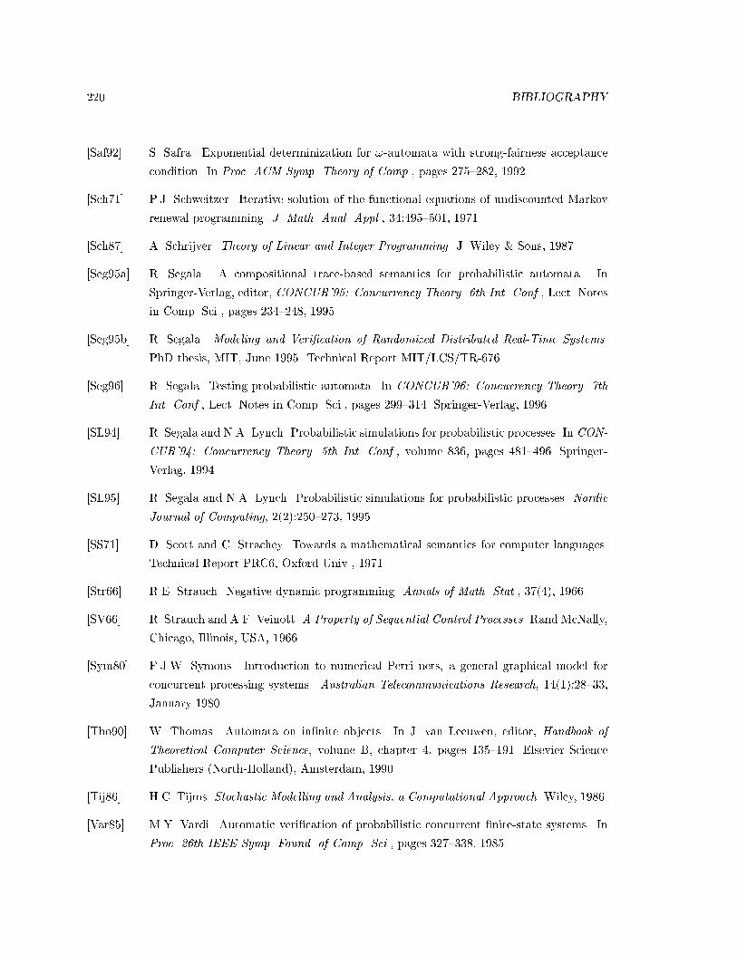
220 BIBLIOGRAPHY
[Saf92] S. Safra. Exponential determinization for !-automata with strong-fairness acceptance
condition. In Proc. ACM Symp. Theory of Comp., pages 275{282, 1992.
[Sch71] P.J. Schweitzer. Iterative solution of the functional equations of undiscounted Markov
renewal programming. J. Math. Anal. Appl., 34:495{501, 1971.
[Sch87] A. Schrijver. Theory of Linear and Integer Programming. J. Wiley & Sons, 1987.
[Seg95a] R. Segala. A compositional trace-based semantics for probabilistic automata. In
Springer-Verlag, editor, CONCUR'95: Concurrency Theory. 6th Int. Conf., Lect. Notes
in Comp. Sci., pages 234{248, 1995.
[Seg95b] R. Segala. Modeling and Veri�cation of Randomized Distributed Real-Time Systems.
PhD thesis, MIT, June 1995. Technical Report MIT/LCS/TR-676.
[Seg96] R. Segala. Testing probabilistic automata. In CONCUR'96: Concurrency Theory. 7th
Int. Conf., Lect. Notes in Comp. Sci., pages 299{314. Springer-Verlag, 1996.
[SL94] R. Segala and N.A. Lynch. Probabilistic simulations for probabilistic processes. In CON-
CUR'94: Concurrency Theory. 5th Int. Conf., volume 836, pages 481{496. Springer-
Verlag, 1994.
[SL95] R. Segala and N.A. Lynch. Probabilistic simulations for probabilistic processes. Nordic
Journal of Computing, 2(2):250{273, 1995.
[SS71] D. Scott and C. Strachey. Towards a mathematical semantics for computer languages.
Technical Report PRC6, Oxford Univ., 1971.
[Str66] R.E. Strauch. Negative dynamic programming. Annals of Math. Stat., 37(4), 1966.
[SV66] R. Strauch and A.F. Veinott. A Property of Sequential Control Processes. Rand McNally,
Chicago, Illinois, USA, 1966.
[Sym80] F.J.W. Symons. Introduction to numerical Petri nets, a general graphical model for
concurrent processing systems. Australian Telecommunications Research, 14(1):28{33,
January 1980.
[Tho90] W. Thomas. Automata on in�nite objects. In J. van Leeuwen, editor, Handbook of
Theoretical Computer Science, volume B, chapter 4, pages 135{191. Elsevier Science
Publishers (North-Holland), Amsterdam, 1990.
[Tij86] H.C. Tijms. Stochastic Modelling and Analysis, a Computational Approach. Wiley, 1986.
[Var85] M.Y. Vardi. Automatic veri�cation of probabilistic concurrent �nite-state systems. In
Proc. 26th IEEE Symp. Found. of Comp. Sci., pages 327{338, 1985.

BIBLIOGRAPHY 221
[Vei69] A.F. Veinott. On discrete dynamic programming with sensitive discount optimality
criteria. Ann. Math. Stat., 40:1635{1660, 1969.
[vGSST90] R. van Glabbeek, S.A. Smolka, B. Ste�en, and C.M.N. Tofts. Reactive, generative, and
strati�ed models of probabilistic processes. In Proc. 5th IEEE Symp. Logic in Comp.
Sci., 1990.
[vGSST95] R. van Glabbeek, S.A. Smolka, B. Ste�en, and C.M.N. Tofts. Reactive, generative, and
strati�ed models of probabilistic processes. Information and Computation, 121(1):59{80,
1995. Preliminary report in LICS'90.
[VW86] M.Y. Vardi and P. Wolper. An automata-theoretic approach to automatic program
veri�cation. In Proc. First IEEE Symp. Logic in Comp. Sci., pages 332{344, 1986.
[Wil91] D. Williams. Probability With Martingales. Cambridge University Press, 1991.
[WL92] Y. Wang and K. Larsen. Testing probabilistic and nondeterministic processes. In Protocol
Speci�cation, Testing, and Veri�cation XII, 1992.
[WSS94] S.-H. Wu, S.A. Smolka, and E.W. Stark. Composition and behaviors of probabilistic
I/O automata. In Springer-Verlag, editor, CONCUR'94: Concurrency Theory. 5th Int.
Conf., Lect. Notes in Comp. Sci., pages 511{528, 1994.
[YCDS94] S. Yuen, R. Cleaveland, Z. Dayar, and S.A. Smolka. Fully abstract characterizations of
testing preorders for probabilistic processes. In CONCUR'94: Concurrency Theory. 5th
Int. Conf., Lect. Notes in Comp. Sci., pages 497{512. Springer-Verlag, 1994.