Centre for Marine Science and Technology

Internal Report

Hydrodynamic tests on a fixed plate in uniform flow

By: Kim Klaka

REPORT C2003-14 9 July 2003 CENTRE FOR MARINE SCIENCE AND TECHNOLOGY CURTIN UNIVERSITY OF TECHNOLOGY PERTH, WESTERN AUSTRALIA

1

HYDRODYNAMIC TESTS ON A FIXED PLATE IN UNIFORM FLOW

CONTENTS

1 Aims............................................................................................................................. 2 2 Background .................................................................................................................. 2

2.1 Context of the experiment.................................................................................... 2 2.2 Previous work ...................................................................................................... 2 2.3 A note on terminology ......................................................................................... 2

3 Methodology ................................................................................................................ 5 3.1 Parameter space ................................................................................................... 5 3.2 Scaling.................................................................................................................. 5 3.3 Blockage .............................................................................................................. 6

4 Equipment .................................................................................................................... 7 4.1 Facility ................................................................................................................. 7 4.2 Plates .................................................................................................................... 8 4.3 Experimental rig................................................................................................... 8 4.4 Instrumentation .................................................................................................... 9 4.5 Strain gauges........................................................................................................ 9

5 Procedure ................................................................................................................... 11 5.1 Calibration.......................................................................................................... 11 5.2 Test runs............................................................................................................. 11 5.3 Data Processing.................................................................................................. 12

6 Errors.......................................................................................................................... 13 6.1 Gauge signals ..................................................................................................... 13 6.2 Gauge calibration ............................................................................................... 13 6.3 Flow velocity ..................................................................................................... 14 6.4 Other errors ........................................................................................................ 14 6.5 Error estimation and propagation....................................................................... 14

7 Results and discussion ............................................................................................... 15 7.1 Drag.................................................................................................................... 15

7.1.1 Effect of flow speed ................................................................................... 15 7.1.2 Effect of plate angle ................................................................................... 19 7.1.3 Effect of plate geometry............................................................................. 20

7.2 Lift...................................................................................................................... 21 7.3 Roll moment....................................................................................................... 21 7.4 Centre of pressure .............................................................................................. 22

8 Conclusions................................................................................................................ 23 9 References.................................................................................................................. 23

2

1 AIMS

The aim of the test program was to measure the hydrodynamic forces acting on flat plates at near-normal angles to the flow. Variables investigated were flow speed, plate angle and plate aspect ratio.

2 BACKGROUND

2.1 Context of the experiment

A research program is being conducted to predict the roll motion of a yacht at zero ship speed in a low amplitude ocean wave field, in both deep and shallow water. Computer predictions, full scale trials and model experiments were carried out, focussing on the damping effect of the keel, which can be modelled as a flat plate oscillating normal to the flow (Klaka, 2000), (Klaka, 2001). In order to investigate further, a forced oscillation rig was built to measure the forces and moments generated by a range of flat plates in calm water in various water depths (Klaka, 2003). The facility used was an open circulating water channel. The opportunity therefore presented itself to measure the forces on the plates when stationary in uniform flow.

2.2 Previous work

The proposed experiment was intended to extend the very limited data set for the forces on surface piercing flat plates at near-normal angles to uniform flow.

Open channel flows have been studied extensively with obstructions emanating from the channel floor (Webber, 1971), (Massey, 1979), but few data exist for surface-suspended obstructions which relate to the problem at hand. Studies have been conducted on the flow under a gate ((Chaudhry, 1993) p.180), but they were for flows with substantially different water levels either side of the gate, where hydraulic jumps may occur. Most work on such objects focussed on water depth and velocity changes rather than the forces exerted on the plate. One of the few relevant data sets was that of Hay, reported in page 10-15 of (Hoerner, 1965). This showed the drag coefficient of a surface piercing flat plate normal to the flow as a function of plate-depth based Froude number, for a range of plate aspect ratios. Unfortunately the definition of aspect ratio provided was ambiguous.

2.3 A note on terminology

The research described was conducted by the author whilst enrolled in a doctoral program in the Department of Applied Physics at Curtin University. The thesis topic lies in the field of naval architecture, generally considered a branch of engineering for the most part. The terminology adopted was that most commonly used in engineering and, where practicable, symbols and sign conventions followed the recommendations of the International Towing Tank Conference (Johnson, 1999). In an endeavour to make this work accessible to a readership in the fields of both engineering and science, some of the terms used are described below in greater detail than might be found in work pertaining to a single discipline.

3

• Sign conventions

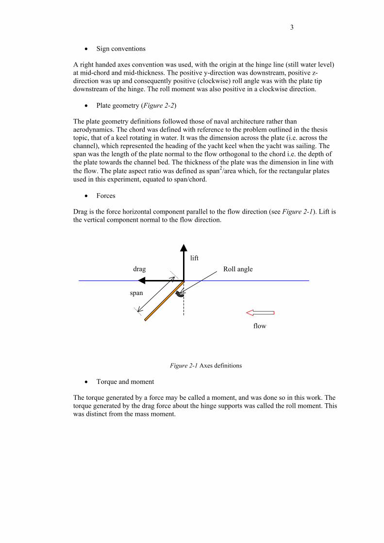
A right handed axes convention was used, with the origin at the hinge line (still water level) at mid-chord and mid-thickness. The positive y-direction was downstream, positive z-direction was up and consequently positive (clockwise) roll angle was with the plate tip downstream of the hinge. The roll moment was also positive in a clockwise direction.

• Plate geometry (Figure 2-2)

The plate geometry definitions followed those of naval architecture rather than aerodynamics. The chord was defined with reference to the problem outlined in the thesis topic, that of a keel rotating in water. It was the dimension across the plate (i.e. across the channel), which represented the heading of the yacht keel when the yacht was sailing. The span was the length of the plate normal to the flow orthogonal to the chord i.e. the depth of the plate towards the channel bed. The thickness of the plate was the dimension in line with the flow. The plate aspect ratio was defined as span2/area which, for the rectangular plates used in this experiment, equated to span/chord.

• Forces

Drag is the force horizontal component parallel to the flow direction (see Figure 2-1). Lift is the vertical component normal to the flow direction.

Figure 2-1 Axes definitions

• Torque and moment

The torque generated by a force may be called a moment, and was done so in this work. The torque generated by the drag force about the hinge supports was called the roll moment. This was distinct from the mass moment.

drag

span

lift

flow

Roll angle

4

Plate 2

Plate 4

span

chord

Plate 1

0.3m

0.205m

Figure 2-2. Plate geometry

5

3 METHODOLOGY

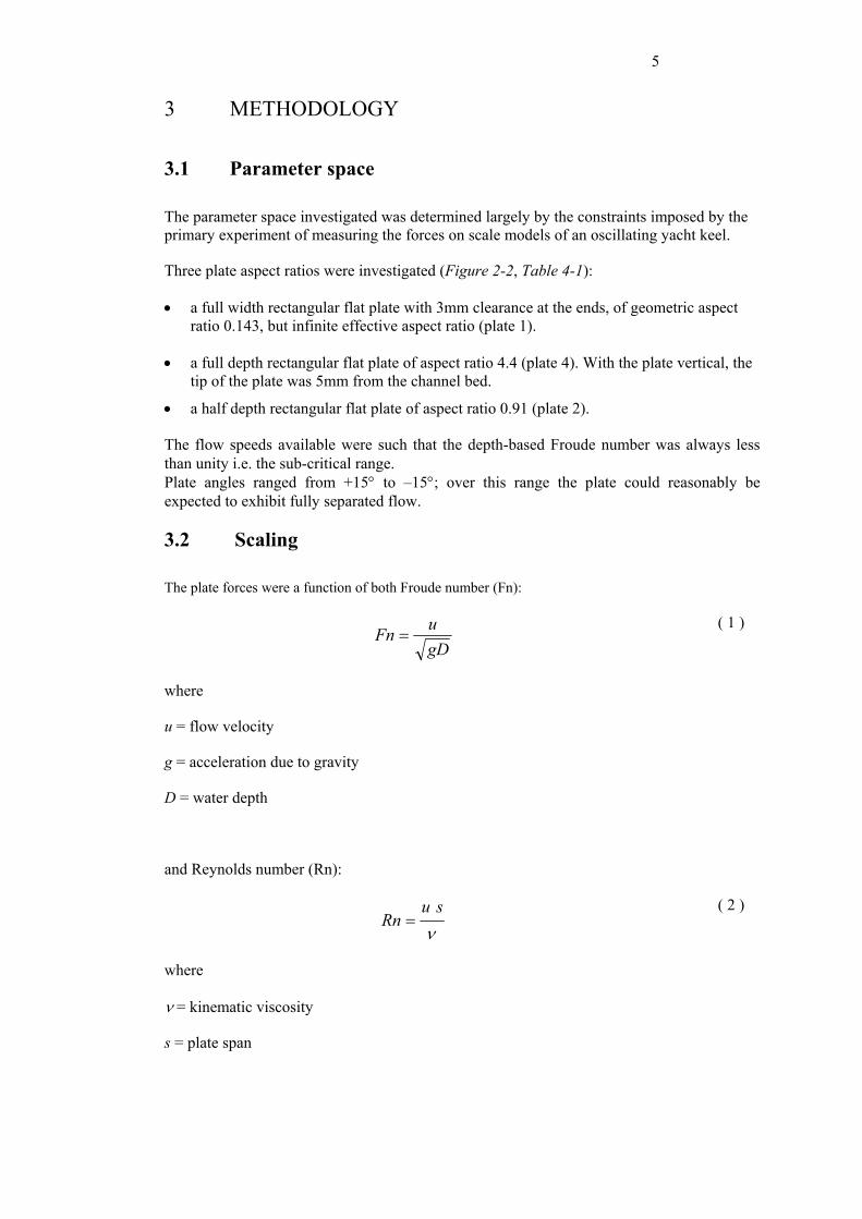
3.1 Parameter space

The parameter space investigated was determined largely by the constraints imposed by the primary experiment of measuring the forces on scale models of an oscillating yacht keel.

Three plate aspect ratios were investigated (Figure 2-2, Table 4-1):

• a full width rectangular flat plate with 3mm clearance at the ends, of geometric aspect ratio 0.143, but infinite effective aspect ratio (plate 1).

• a full depth rectangular flat plate of aspect ratio 4.4 (plate 4). With the plate vertical, the tip of the plate was 5mm from the channel bed.

• a half depth rectangular flat plate of aspect ratio 0.91 (plate 2).

The flow speeds available were such that the depth-based Froude number was always less than unity i.e. the sub-critical range. Plate angles ranged from +15° to –15°; over this range the plate could reasonably be expected to exhibit fully separated flow.

3.2 Scaling

The plate forces were a function of both Froude number (Fn):

gDuFn =

( 1 )

where

u = flow velocity

g = acceleration due to gravity

D = water depth

and Reynolds number (Rn):

νsu

Rn = ( 2 )

where

ν = kinematic viscosity

s = plate span

6

Forces and moments were non-dimensionalised as follows:

2

21 Au

forceC force

ρ=

( 3 )

sAu

momentCmoment2

21 ρ

= ( 4 )

where

A = plate profile area

ρ = water density

Under Froude scaling the inertial effects would be correctly scaled. The Reynolds number would change but the effects are usually quite small if there is a significant amount of separated flow and the separation points do not change with Reynolds number (Hoerner, 1965), (Hoerner and Borst, 1975). In such circumstances the non-dimensionalised forces and moments may be compared directly for experiments conducted at the same Froude number. Nevertheless care should be taken when comparing results from experiments conducted at significantly different Reynolds number. Further, caution is urged to check that the non-dimensionalising parameters used are the same.

3.3 Blockage

An object placed in a channel will experience different forces compared with the same object placed in unrestricted flow. This effect is known as blockage, and is reasonably well understood in wind tunnels (Rae and Pope, 1984), (Pankhurst and Holder, 1965) and towing tanks (Scott, 1976), (Harvald, 1983). The blockage effects for this experiment are related to, but not the same as, wind tunnel effects and towing tank effects.

Blockage effects may be divided as follows:

Wall boundary layer effects.

The progressive thickening of the boundary layer along the length of the channel wall causes a decrease in the static pressure downstream, hence the velocity increases to maintain flow rate continuity. This effect is important in wind tunnels but is considered negligible for water tests because the boundary layer thickness is proportionally much smaller.

Solid blocking

The presence of the plate in the channel reduces the area through which water may flow. For a closed channel e.g. a wind tunnel, the effect is much less than (approximately 25% of) the amount calculated by applying Bernoulli’s equation, despite the average velocity change being accurately predicted. This is because the displacement of the streamlines is greater as you move further away from the plate, but the forces related to that change decrease with distance from the plate (Rae and Pope, 1984) p353. The mathematical approach to calculating solid blockage is by the method of images, using doublets. This method becomes quite complicated when a free surface is present, and was not considered suitable for this experiment. Given that the free surface provides a pressure relief, the wind tunnel solid

7

blocking calculations provide an upper threshold estimate of this blockage component, rather than an accurate estimate.

Wake blocking

The mean velocity in the wake will be lower than the free stream velocity; however, the velocity outside the wake in a closed channel must be higher than the free stream in order to maintain continuity of volume flow rate. This higher velocity will, from Bernoulli’s theorem, decrease the pressure in the wake region and create an additional drag force. This is computed for wind tunnels by using a line source (across the channel) to represent the wake-generating trailing edge. The simulated wake is contained within the channel by adding an infinite vertical row of source-sink combinations, producing a net horizontal velocity. As with solid blocking, this method is not practical when a free surface is present, rather it provides an order of magnitude upper value estimate of the wake blockage.

Streamline curvature

The curvature of streamlines that occurs around any lifting body is restricted by the top and bottom of the channel. This results in an increase in lift compared with the unconstrained flow condition. For this experiment, the free surface yet again relaxes this constraint. The lift generated was very small for the conditions under investigation.

Wave resistance blockage

The wave pattern generated by the plate will be affected by the channel boundaries, particularly the channel bed. This form of blockage is addressed in ship towing tank resistance tests, but in a manner inapplicable to this experiment for the following reasons:

• The methods, all empirically based (e.g. (Scott, 1976), (Scott, 1966)), include all blockage effects in one – including wake and solid blockage.

• The formulae used are based on ship length, a length dimension not appropriate to a plate normal to the flow.

This experiment lies outside the range of data used to develop the empirical blockage formulae with particular regard to object slenderness and channel aspect ratio. This latter is surprisingly important, as shown in the first data subset of table 1 in (Scott, 1976).

4 EQUIPMENT

4.1 Facility

The facility was an Armfield Engineering S5-10 circulating open water channel, with a 10m long working length of cross section 300mm square. The sides are transparent. The channel slope can be varied manually at the upstream end by a screw jack. The water was circulated using a centrifugal pump. The flow rate (and in consequence, the water depth) was regulated by a flow valve. The water depth can be controlled separately by changing the height of a sluice gate at the downstream end.

8

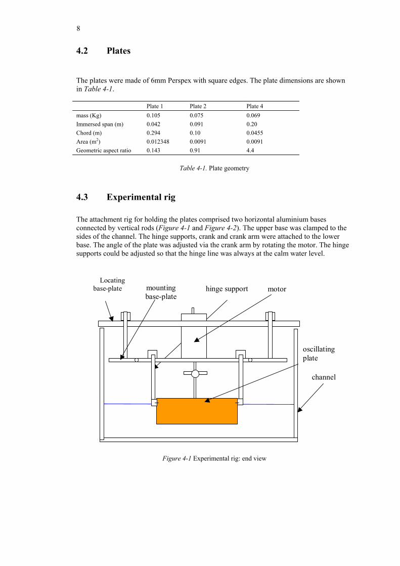
4.2 Plates

The plates were made of 6mm Perspex with square edges. The plate dimensions are shown in Table 4-1.

Plate 1 Plate 2 Plate 4 mass (Kg) 0.105 0.075 0.069 Immersed span (m) 0.042 0.091 0.20 Chord (m) 0.294 0.10 0.0455 Area (m2) 0.012348 0.0091 0.0091 Geometric aspect ratio 0.143 0.91 4.4

Table 4-1. Plate geometry

4.3 Experimental rig

The attachment rig for holding the plates comprised two horizontal aluminium bases connected by vertical rods (Figure 4-1 and Figure 4-2). The upper base was clamped to the sides of the channel. The hinge supports, crank and crank arm were attached to the lower base. The angle of the plate was adjusted via the crank arm by rotating the motor. The hinge supports could be adjusted so that the hinge line was always at the calm water level.

oscillating plate

Locating base-plate mounting

base-platemotor

channel

hinge support

Figure 4-1 Experimental rig: end view

9

crank arm

Figure 4-2 Experimental rig: side view

4.4 Instrumentation

The instrumentation for these experiments comprised 12 strain gauges (see 4.5) and a Pygmy 30mm diameter flow meter to measure flow rate. Water depth was measured using steel rules permanently mounted on the outside of the channel. All signals acquired were analogue DC. The Daqbook system was used and the digitised signals were stored on a PC.

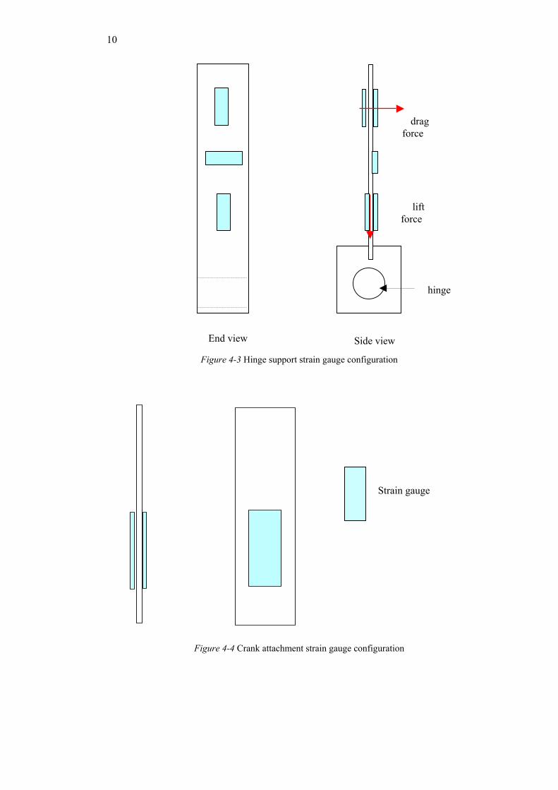
4.5 Strain gauges

The gauges were super-glued to the aluminium substrate then coated in polyurethane. The hinge supports were strain gauged as shown in Figure 4-3. The upper pair were connected as a half-bridge to provide a difference reading for maximum sensitivity to drag-induced bending moment. The signals from the lower pair were recorded individually in order to measure lift force. The transverse gauge provided a check on drag force measurement (through Poisson strain) and any torsional load. Whilst this configuration did not permit decomposition of the readings into all possible load conditions, it did allow for checks to be made for contamination of signals from unexpected load conditions. Cross-axis sensitivity of the gauges was measured during calibration. The crank attachment was gauged with a half bridge pair (Figure 4-4), based on the assumption that the only load was in line with the crank arm.

10

Figure 4-3 Hinge support strain gauge configuration

Figure 4-4 Crank attachment strain gauge configuration

drag force

hinge

End view Side view

lift force

Strain gauge

11

5 PROCEDURE

5.1 Calibration

The strain gauges were calibrated statically by applying known loads to each hinge support and the crank arm connection, in a range of directions. The gauge reading was allowed to stabilise then the mean value taken over typically 5 seconds. The means were plotted and a linear regression performed in order to determine the calibration factor. The offset was not required for calibration as forces were estimated from the difference between signals of a run file and its associated zero-datum file. The calibration process was conducted at two different gain settings for the strain gauges. The maximum load applied was limited by the deflection of the gauge support being large enough to jeopardise the integrity of the bond between gauge and substrate.

5.2 Test runs

The strain gauge circuits were allowed to warm up for typically one hour in order to reduce gauge drift due to temperature variation. The procedure for each run was to set the plate angle by adjusting the motor crank. The angle was measured using an adjustable square. The channel was then filled with water to the correct depth and approximate desired flow speed. This required adjustment of both the flow valve and sluice gate until an appropriate flow speed was attained at a steady state.

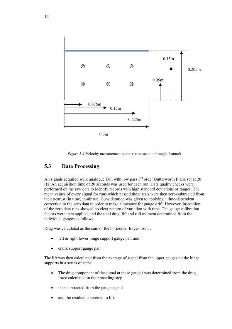
Data acquisition would then start, for 20 seconds duration at 100Hz sample rate. The difference in free surface height between the two faces of the plate was measured using a steel rule. On completion of sampling, the flow speed was measured at 6 transverse locations at a plane 200mm ahead of the plate. The transverse locations are shown in Figure 5-1 and represented the region occupied by the plate and not the region affected by the channel wall boundary layer. On completion of a test run the sluice gate and valve were adjusted for the next flow speed. It was not possible to set the flow speed at a predetermined level, instead velocity increments were estimated by a combination of visual observations and acquired experience of the gate and valve adjustments. Before and after each series of flow speeds, a static calibration run in air was conducted. These runs served as the zero datum for the gauge signals.

The plates were always set with the hinges at the static waterline. All tests were conducted at a water depth of 0.205m.

During each run the digital display of signals was inspected and if a channel reached saturation that run would be discarded, the gains reduced if appropriate, and the run repeated. Runs where readings extended beyond the limits of calibration were also discarded.

A series of runs were conducted without a plate attached to the hinge supports, in order to determine the tare of the supports.

Photos and video footage were taken at various times during the tests.

12

Figure 5-1 Velocity measurement points (cross section through channel)

5.3 Data Processing

All signals acquired were analogue DC, with low pass 3rd order Butterworth filters set at 20 Hz. An acquisition time of 20 seconds was used for each run. Data quality checks were performed on the raw data to identify records with high standard deviations or ranges. The mean values of every signal for runs which passed these tests were then zero-subtracted from their nearest (in time) in-air run. Consideration was given to applying a time-dependent correction to the zero data in order to make allowance for gauge drift. However, inspection of the zero data runs showed no clear pattern of variation with time. The gauge calibration factors were then applied, and the total drag, lift and roll moment determined from the individual gauges as follows:

Drag was calculated as the sum of the horizontal forces from :

• left & right lower hinge support gauge pair and

• crank support gauge pair

The lift was then calculated from the average of signal from the upper gauges on the hinge supports in a series of steps:

• The drag component of the signal at these gauges was determined from the drag force calculated in the preceding step,

• then subtracted from the gauge signal

• and the residual converted to lift.

0.225m

0.075m

0.3m

0.15m

0.05m

0.15m

0.205m

13

• The lift force from the left and right gauges were added to get the total lift force.

Finally, the static force component due to buoyancy (not present in the zero datum in-air runs) was calculated analytically then subtracted from the gauge lift force, to yield the hydrodynamic lift.

The roll moment was determined by taking moments about the hinge support. As with lift force, a buoyancy correction was applied. The hinge support tare was subtracted from the calculated forces. A plot of force as a function of flow velocity revealed a small offset on the y-axis which clearly should not exist. This was removed by firstly finding the power law which yielded the best fit to each series of data, then subtracting the offset of this best fit from each data point. This step was important for the final processing stage – the conversion of forces and moment to dimensionless coefficients – because the denominator contained a velocity squared term which would have introduced large errors at low flow speeds if the zero velocity offset was not removed.

6 ERRORS

6.1 Gauge signals

The physical size of the rig components were small relative to the size of the gauges, so there were errors due to strain gradients, gauge thickness etc. However, these were largely accounted for in the calibration process. Temperature effects were accounted for in two ways. Firstly, by choosing gauges with a thermal expansion coefficient similar to that of the attachment plate. Secondly, by taking measurements over short duration, which were thus unlikely to experience significant change in temperature. Nevertheless, zero datum gauge signals varied substantially over a day’s testing. The fluctuations were not correlated with time from switch on, indicating that temperature variations were not the cause. Residual mechanical loads in the rig are a likely explanation.

The signal generated by a gauge may be the resultant of strains in several different directions. The gauge configuration reduced this contamination and enabled checks to be made on its extent. For example, the transverse gauges on the hinge support would respond to both drag force and torsion (and to a much lesser extent, lift force and any cross-channel signal), whereas the differenced upper gauge pair signal was dominated by strain induced by drag force. Therefore a check for excessive torsion was made by comparison of the signals from the upper pair and the Poisson-strain from the transverse gauge. However, this was not a suitable method for measuring such loads as there was cross-contamination and large errors; rather it provided a useful data quality check on a pass-fail basis.

The lift force signal was generated by the axial load in the hinge supports and determined from the average reading from each of the lower pair of gauges on the hinge supports (see 5.3). The absolute strain values were very low, owing to the necessary stiffness of the supports. Consequently the errors in the lift-induced signal were very large – generally constituting the bulk of the signal.

6.2 Gauge calibration

The coefficient of determination (r2) for the calibration factors used to determine the drag and roll were always greater than 0.999. Cross-coupling between gauges was measured and found to be insignificant, except for the quantifiable instances of Poisson strain. Temperature

14

fluctuations may have affected the calibration factors, though the gauge specifications indicate this would be an error of second order magnitude over the temperature range of the experiments.

6.3 Flow velocity

Measuring the flow speed at 6 locations for each run enabled the standard deviation of the mean of each run to be calculated. There was no evidence for consistent asymmetry in the measurements, indicating that the flow pump was not introducing any mean rotary or off-axis flow at the plate.

The flow meter provided an integrated signal over a 10 second period, averaging out short term fluctuations. The resolution of the meter was 1 unit, which represents 0.051m/s. The flow measurements at the 6 spatial locations were usually taken immediately after the data acquisition period. Thus any longer term time variations were implicit in the spatial variations. On occasions when the spatial variations were repeated, there was no evidence for any trend of variation with time.

6.4 Other errors

Water depth was measured using steel rules permanently mounted on the outside of the channel. The measurement was accurate to within 1mm, but the level occasionally fluctuated from the target value by up to 2mm owing to operational difficulties.

The mean water temperature of 26.3°C varied by +-0.9°C over the period of the tests.

The plate angle measurement was accurate to within +-0.2° with respect to the channel bed. Relative accuracy between plate angles was +-0.1°. The plate was subject to slight flexure, so the angle to the flow in the dynamic condition may have been up to 1° different at the plate tip, compared with the static measurement.

The friction in the bearings for the tests in air was unlikely to be the same as for the test in water at the same frequency, because the bearing load was different.

The effects of blockage are discussed in 3.3. Given the uncertainty in estimating blockage effects for the current experiment, the results have been left uncorrected. This should be borne in mind when comparing with other experiments, particularly those conducted at different model:tank area ratios.

6.5 Error estimation and propagation

The error estimate comprised the following components:

• signal in uniform flow

• in-air datum signal

• calibration

• tare correction

• for coefficients, estimates of the force/moment denominator errors.

15

Errors for the uniform flow signals were calculated from the signal standard deviation for the run. Errors for the in-air datum signal were estimated from the standard deviation of the datum readings over a day’s testing at uniform gain setting. Calibration errors were estimated from the standard deviations of the time series of the calibration signals. Tare errors were estimated as the same as for a low speed flow run. The errors from these sources were propagated through to the forces and moments. The errors in the flow velocity were determined from the standard deviation of the spatial measurements. Errors due to time variation of velocity were not independent of the errors in the time series of the gauge signals, so were not estimated separately. The velocity error estimate, and those of the other denominators in the non-dimensional coefficients, were then propagated to yield errors in the coefficients. A summary of error magnitudes for drag is given in Table 6-1; roll moment errors were of similar proportion. Lift force standard deviations were difficult to estimate accurately, but appear to be over 50% for most conditions, decreasing with flow speed.

It was clear from the error propagation process that the relative values of the errors were greater at lower flow speeds because the amplitude of the zero datum and tare corrections were then of the same order as the uniform flow signal. The largest source of error for most conditions was from the zero datum. Flow velocity and plate immersed area errors were also significant. The errors in instrument calibration were two orders of magnitude less than other error sources.

Low speed (Fn =0.161) High speed (Fn = 0.364)

Standard deviation mean Standard deviation. mean

drag (N) 0.031 0.11 0.064 1.9

drag coefficient 0.33 1.29 0.05 1.72

Table 6-1 error estimates: plate 1, 10° angle

7 RESULTS AND DISCUSSION

7.1 Drag

7.1.1 Effect of flow speed

Figure 7-1, Figure 7-2 and Figure 7-3 show the drag coefficient varies only slightly with Froude number for all three plates tested.

16

plate 1

0

0.5

1

1.5

2

2.5

3

3.5

4

4.5

5

0 0.05 0.1 0.15 0.2 0.25 0.3 0.35 0.4 0.45

Fn

Cd 0 deg

5 deg10 deg15 deg-5 deg-10 deg-15 deg

90% conf. limit

Figure 7-1 Drag coefficient as a function of Froude number; plate 1

plate 2 (square)

0

0.5

1

1.5

2

2.5

3

3.5

4

4.5

0 0.05 0.1 0.15 0.2 0.25 0.3 0.35 0.4 0.45

Fn

Cd

0 deg5 deg10 deg15 deg20 deg-5 deg-10 deg-15 deg

90% conf. limit

Figure 7-2 Drag coefficient as a function of Froude number; plate 2

17

plate 4

0

1

2

3

4

5

6

7

8

9

10

0 0.05 0.1 0.15 0.2 0.25 0.3 0.35

Fn

Cd

0 deg5 deg10 deg15 deg-5 deg-10 deg-15 deg

90% conf. limit

Figure 7-3 Drag coefficient as a function of Froude number; plate 4

In order to illustrate the effect more closely, the best-fit drag-velocity exponents are shown in Figure 7-4. The mean value of the exponent for all conditions was 2.07, with a range of 1.76 to 2.41 (with one outlier at 1.15). If there were no Reynolds number, blockage or free surface effects, the exponent would be expected to hold a value of 2. The small variation from this figure implies that such effects are relatively modest.

The magnitude of the drag coefficient was in the region 1.8 to 2.3, somewhat higher than the value of 1.2 for a plate normal to the flow in an unconfined flow (Newman, 1977). This may be due to the free surface effect; however, such an effect would be expected to increase with Froude number, as evidenced by Hay in (Hoerner, 1965) p10-15. The maximum drag coefficient found by Hay was 1.6, occurring at Froude numbers greater than 1. Hoerner considered these high values to be a consequence of wave drag. The free surface distortion measured in the current experiments supported this hypothesis (Figure 7-5, Figure 7-6 and Figure 7-7), but the independence of drag coefficient from Froude number implies either a false hypothesis or some other effect counteracting the wave drag increase – possibly a free-surface blockage change.

18

effect of angle on drag v speed powerlaw (drag = vel^n)

1

1.2

1.4

1.6

1.8

2

2.2

2.4

2.6

-20 -15 -10 -5 0 5 10 15

angle (deg)

n

plate 1

plate 2

plate 4

Figure 7-4 Power law variation with angle and plate geometry

plate 1

0

8

16

24

32

40

0.05 0.1 0.15 0.2 0.25 0.3 0.35 0.4

Fn

step

(mm

)

0 deg5 deg10 deg15 deg-5 deg-10 deg-15 deg

90% conf. limit

Figure 7-5 Hydraulic step height as a function of Froude number; plate 1

19

plate 2 (square)

0

8

16

24

32

40

0.05 0.1 0.15 0.2 0.25 0.3 0.35 0.4

Fn

step

(mm

)-5 deg

-10 deg

-15 deg

90% conf. limit

Figure 7-6 Hydraulic step height as a function of Froude number; plate 2

plate 4

0

8

16

24

32

40

0.05 0.1 0.15 0.2 0.25 0.3 0.35 0.4

Fn

step

(mm

)

0 deg5 deg10 deg15 deg-5 deg-10 deg-15 deg

90% conf.limit

Figure 7-7 Hydraulic step height as a function of Froude number; plate 4

7.1.2 Effect of plate angle

Figure 7-1, Figure 7-2 and Figure 7-3 show the effect of plate angle on drag was small. A sample crossplot is presented in Figure 7-8. The variation of the drag-velocity exponent with angle, illustrated in Figure 7-4 indicated no clear trend.

20

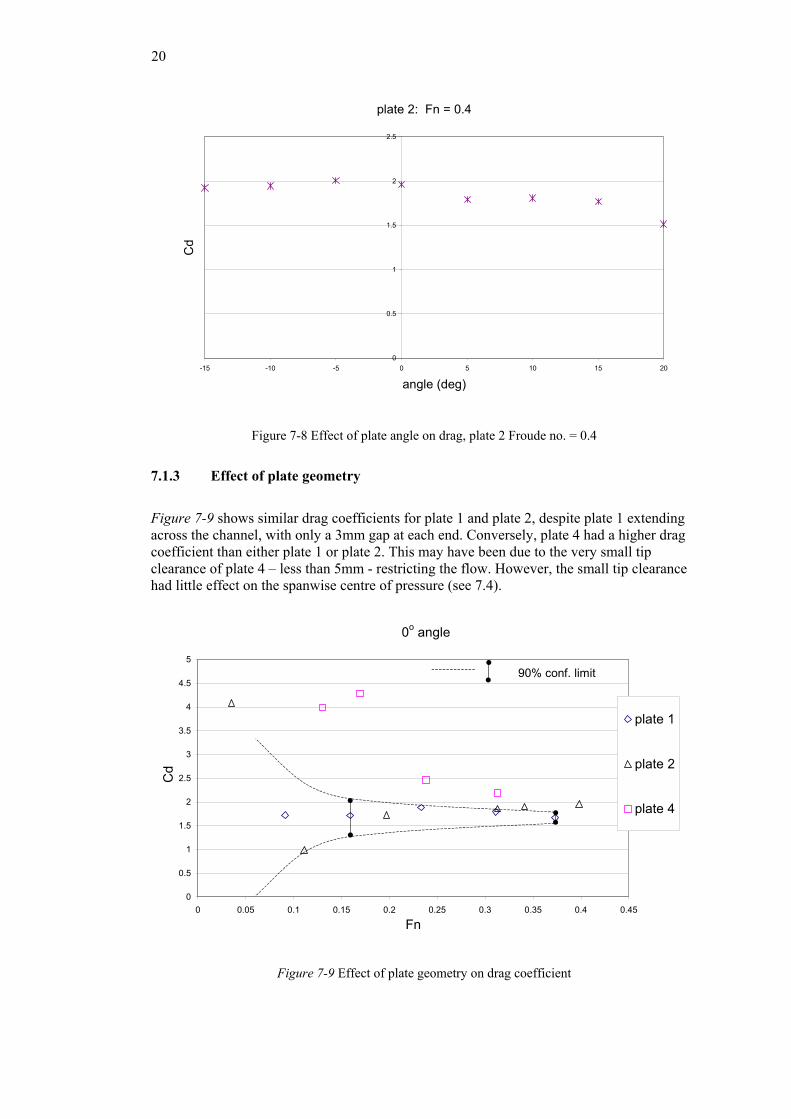
plate 2: Fn = 0.4

0

0.5

1

1.5

2

2.5

-15 -10 -5 0 5 10 15 20

angle (deg)

Cd

Figure 7-8 Effect of plate angle on drag, plate 2 Froude no. = 0.4

7.1.3 Effect of plate geometry

Figure 7-9 shows similar drag coefficients for plate 1 and plate 2, despite plate 1 extending across the channel, with only a 3mm gap at each end. Conversely, plate 4 had a higher drag coefficient than either plate 1 or plate 2. This may have been due to the very small tip clearance of plate 4 – less than 5mm - restricting the flow. However, the small tip clearance had little effect on the spanwise centre of pressure (see 7.4).

0o angle

0

0.5

1

1.5

2

2.5

3

3.5

4

4.5

5

0 0.05 0.1 0.15 0.2 0.25 0.3 0.35 0.4 0.45

Fn

Cd

plate 1

plate 2

plate 4

90% conf. limit

Figure 7-9 Effect of plate geometry on drag coefficient

21

7.2 Lift

The results for lift force and lift coefficient were prone to very large errors, owing to the insensitivity of the gauges to the very low axial strains in the hinge supports (see 6). Most of the lift coefficients recorded in this experiment ranged between 2 and 4. Lift coefficients in other flow regimes rarely exceed 1.5 (Hoerner, 1965).

7.3 Roll moment

Roll moment variation followed generally similar trends to that for drag. An example is shown in Figure 7-10.

plate 2 (square)

0

0.2

0.4

0.6

0.8

1

1.2

1.4

1.6

1.8

2

0 0.05 0.1 0.15 0.2 0.25 0.3 0.35 0.4 0.45Fn

Cϕ

0 deg5 deg10 deg15 deg20 deg-5 deg-10 deg-15

90% conf. limit

Figure 7-10 Variation of roll moment coefficient for plate 2

The corresponding power law dependency is shown in Figure 7-11, the mean value of the exponent being 1.91.

22

effect of angle on roll v speed powerlaw (roll = vel^n)

1

1.2

1.4

1.6

1.8

2

2.2

2.4

-20 -15 -10 -5 0 5 10 15

angle (deg)

n

plate 1 plate 2 plate 4

Figure 7-11 Roll moment power law variation for plate 2

7.4 Centre of pressure

The spanwise centre of pressure was estimated from the ratio of roll moment to drag force. This did not take account of lift force, but the contribution of lift to roll moment was small over the range of roll angles tested. It was considered that the very large errors in the lift estimates would create great uncertainty if they were included in the calculation. The results for 0° roll angle (at which the lift influence was zero) are shown in Figure 7-12. The position was close to 50% of plate span, as might be expected for a fully immersed plate. This suggests the effect of the free surface on force generation was either small, or uniform down the span of the plate. The effect on centre of pressure of the small tip clearance of plate 4 was also very small.

23

0o angle

0

20

40

60

80

100

120

0 0.05 0.1 0.15 0.2 0.25 0.3 0.35 0.4 0.45

Fn

Cp

(% s

pan)

plate 1

plate 2

plate 4

90% conf. limit

Figure 7-12 Spanwise centre of pressure at 0° angle

8 CONCLUSIONS

For the conditions of the experiment, and within the limits of experimental error, the following conclusions were drawn:

• Drag and roll moment varied approximately as flow speed squared for all plates investigated.

• The influence of plate angle on drag coefficient was small, with no clear trend.

• The magnitude of the drag coefficients for the surface-piercing plates was greater than for published data on fully submerged plates.

• The centre of pressure was at approximately 50% of the span.

9 REFERENCES

Chaudhry, M. H. (1993) Open-channel flow, Prentice Hall, New Jersey.

Harvald, S. A. (1983) Resistance and propulsion of ships, Wiley, New York.

Hoerner, S. F. (1965) Fluid dynamic drag, Hoerner Fluid Dynamics, Bricktown USA.

Hoerner, S. F. and Borst, H. V. (1975) Fluid dynamic lift, Hoerner Fluid Dynamics, Bricktown, USA.

Johnson, B. (1999) ITTC symbols and terminology list, U.S. Naval Academy.

24

Klaka, K. (2000) Response of a vessel to waves at zero ship speed: preliminary full scale experiments, CMST 2000-21 Centre for Marine Science & Technology, Curtin University 28.

Klaka, K. (2001) Model tests on a circular cylinder with appendages, CMST 2001-14 Centre for Marine Science & Technology, Curtin University of Technology 26.

Klaka, K. (2003) Hydrodynamic tests on a plate in forced oscillation, 2003-06 Centre for Marine Science and Technology, Curtin University 44.

Massey, B. S. (1979) Mechanics of fluids, Van Nostrand Reinhold.

Newman, N. J. (1977) Marine hydrodynamics, MIT Press, Cambridge Massachusetts.

Pankhurst, R. C. and Holder, D. W. (1965) Wind-tunnel technique, Pitman, London.

Rae, W. H. and Pope, A. (1984) Low-speed wind tunnel testing, John Wiley & Sons.

Scott, J. R. (1966) A blockage corrector Transactions Royal Institution of Naval Architects, 108, 153-163.

Scott, J. R. (1976) Blockage correction at sub-critical speeds Transactions Royal Institution of Naval Architects, 118, 169-179.

Webber, N. B. (1971) Fluid mechanics for civil engineers, Chapman & Hall, London.