Centre for Efficiency and Productivity Analysis

Working Paper Series No. WP07/2016

Slack-based directional distance function in the presence of bad outputs: Theory and Application to Vietnamese Banking

Manh D. Pham, Valentin Zelenyuk

Date: November 2016

School of Economics University of Queensland

St. Lucia, Qld. 4072 Australia

ISSN No. 1932 - 4398

Slack-based directional distance function in the

presence of bad outputs: Theory and Application to

Vietnamese Banking

Manh D. Pham⇤1 and Valentin Zelenyuk1,2

1School of Economics, The University of Queensland, Australia

2Centre for E�ciency and Productivity Analysis, The University of Queensland, Australia

November 16, 2016

Abstract

In this paper we extend the slack-based directional distance function intro-

duced by Fare and Grosskopf (2010) to measure e�ciency in the presence of bad

outputs and illustrate it through an application on data of Vietnamese commer-

cial banks. We also compare results from the slack-based directional distance

function relative to the directional distance function, the enhanced hyperbolic

e�ciency measure (Fare et al., 1989) and the Farrell-type technical e�ciency

and confirm that it has greater discriminative power.

Key words: Banking, Bad outputs, Data Envelopment Analysis, Directional distance

function, Slack-based e�ciency, Performance analysis.

JEL classification: C14, C15, C44, D24, G21

⇤Corresponding author. Email address: ducmanh.pham@uq.net.au

1

1 Introduction

It is widely conceded that financial system has a strong influence on the functioning of

economy. Indeed, a comment of William Gladstone, the former British Prime Minister,

in 1858 is a stark example: “Finance is, as it were, the stomach of the country, from

which all the other organs take their tone”(Ratcli↵e, 2011). Another illustration is the

2008 Global Financial Crisis that led to the disruption of a huge number of companies

all over the world, illustrating how adversely economies can su↵er from the instabil-

ity of financial systems. As banks play a key role for the health of financial systems,

measuring e�ciency of banking industry is essential for devising relevant policies and

regulations.

In their recent survey, Fethi and Pasiouras (2010) pointed out that Data Envelopment

Analysis (DEA) is the most commonly used technique in assessing bank performance.

When looking at the world of DEA, it is well-known that popular radial e�ciency

measures, e.g., the Farrell-type technical e�ciency (Farrell, 1957), possess a number of

drawbacks. First, as pointed out in several works, e.g., Fare and Lovell (1978), radial

measures compute e�ciency scores on the basis of the isoquant, not the e�cient subset

of the technology. Second, traditional e�ciency measures cannot deal with negative

values in the data without transformations which, as Portela et al. (2004) argued, make

it hard to interpret the results since di↵erent types of transformations may lead to dif-

ferent estimates of e�ciency scores.

Furthermore, in the banking sector, undesirable outputs such as non-performing loans

(NPLs) require special attention as they can adversely a↵ect banks’ performance. In-

deed, not only do NPLs lower profit but they may also jeopardize cash flows from

operation, putting banks in a liquidity crisis or even more severely, an insolvent sit-

uation.1 However, only a relatively small portion of studies extensively consider the

undesirable outputs in modeling bank e�ciency. For example, Fukuyama and Weber

(2010) examined the e�ciency of Japanese banks for a two-stage system with bad out-

puts using a slack-based measure. Recently, Lozano (2016) summarized network DEA

applications to bank e�ciency measurement and also proposed a general network slack-

based approach to assess e�ciency at the bank level and at the branch level where bad

outputs are taken into consideration.

1If we view banks as financial intermediaries who take deposits from customers to fund for loans,NPLs are bad outputs that incur losses since banks cannot collect related interests/fees as scheduledwhereas they still have to pay interests to depositors. In addition, banks have to put aside an amountof their money to make provisions for credit losses regarding loans made. This will be discussed furtherin section 4.

2

In this paper we are particularly interested in the slack-based directional distance func-

tion (SD) proposed by Fare and Grosskopf (2010). More recently, Fare et al. (2015)

pointed out that SD approach satisfies four important properties: (i) units invariant,

(ii) monotone, (iii) translation invariant, and (iv) reference set invariant. Besides, as

the SD has been recently introduced, theoretical frameworks for applying this measure

in the DEA context have not been developed relative to the traditional Farrell-type

measure, particularly where bad outputs are taken into consideration. Hence, we in-

tend to fill this gap here to some extent.

In a nutshell, this study aims to achieve three major goals: (i) develop a theoreti-

cal framework for measuring e�ciency by the SD in the presence of bad outputs, (ii)

investigate the di↵erences between the SD and other e�ciency measures, focusing on

their ability in distinguishing individual firms, and (iii) apply the developed framework

to study the e�ciency of Vietnamese commercial banks.2

The rest of the paper is structured as follows. Section 2 provides a general picture

of the Vietnamese banking system. Section 3 establishes the methodology for comput-

ing e�ciency scores using the SD measure in the presence of bad outputs. Section 4

presents decompositions of revenue e�ciency using the SD measure. Section 5 present

an empirical illustration of the developed methodology using a dataset on Vietnamese

commercial banks. Section 6 summarizes important points in this paper and give some

hints to policy-makers.

2 Background on the Vietnamese banking industry

The Vietnamese banking industry has undergone about seven decades of construction

and development since the first establishment of The State Bank of Vietnam (SBV) in

1951. According to The State Bank of Vietnam (2016b), there are 44 commercial banks

operating in Vietnam as of 31 December 2015, including: (i) 7 state-owned commercial

banks,3 (ii) 28 joint-stock commercial banks, (iii) 5 wholly foreign-owned banks and

(iv) 4 joint-venture banks. There are also 2 policy banks and one co-operative bank in

the system.

In general, it is observed that the Vietnamese banking system has been exposed to

some weaknesses in recent years. First, the problem of NPLs is particularly puzzling in

Vietnam. On 12 July 2012, SBV informed that the NPL ratio of the whole Vietnamese

2There is also a wide variety of other approaches for studying productivity and e�ciency in thebanking industry, e.g., Berger and Mester (2003); Du et al. (2015); Curi et al. (2015); Zelenyuk andZelenyuk (2015).

3These are banks where state ownership is over 50% of charter capital.

3

banking system as of 31 March 2012 was 8.6%, significantly higher than a common

reference rate 3%.4 Loans involving real estates and stocks might be one of the reasons

behind this situation. In fact, the increasing amounts of loans for investments in real

estates and stocks and loans collateralized by real estates in the past years might lead

to “bubbles” which adversely a↵ected banks when the real estate and stock market

underwent a downturn.

(a) Number of banks (2011 and 2015) (b) Interest rates in 2008-2014 (%/year)

Figure 1: Number of banks and interest rates in the Vietnamese banking industry.Note: The figures area drawn based on information from SBV (2008; 2009; 2010; 2011; 2012;2013; 2014)

Second, the Vietnamese banking system also witnessed a rapid increase in the number of

credit institutions together with complicated cross-ownership and severe competition.

Escalations in interest rates for deposits from customers well illustrate the competition

in the Vietnamese banking industry in that period of time. Indeed, the rates for de-

posits in Vietnam Dong gradually climbed to approximate 15.6% at the end of June

2011, higher than at the end of 2010 (12.44%) and the cap set by the government at

that time (14%) (The State Bank of Vietnam, 2011).5

In order to strengthen the Vietnamese financial system, the government determined

to restructure the whole banking system, focusing on reducing the number of com-

mercial banks by a package of solutions including eliminating unhealthy banks and

merging several banks. This aim was materialized in the Scheme on “Restructuring

the credit institutions system in the 2011-2015 period”.6 On implementing the Scheme,

4For example, see Circular No. 36/2014/TT-NHNN dated November 20, 2014 of The State Bankof Vietnam where the NPL rate of 3% was set as one of requirements for some banking activities.Another example can be found in Directive No. 02/CT-NHNN dated January 27, 2015 of The StateBank of Vietnam.

5For more details, see Circular No. 02/2011/TT-NHNN dated March 03, 2011, Circular No.30/2011/TT-NHNN dated September 28, 2011 and Directive No. 02/CT-NHNN dated September 07,2011 of The State Bank of Vietnam.

6The Scheme was approved by the Vietnamese Prime Minister in the Decision No. 254/QD-TTg

4

several actions have been taken by the government, resulting in: (i) the nine weakest

commercial banks being identified and restructured during 2011-2012, (ii) the number

of pairs of banks who cross-own each other reduced from 7 pairs in 2012 to 3 pairs

in June 2015, (iii) 493,000 billions VND of NPLs were tackled from 2012 to 2015, re-

ducing the NPL ratio to 2.55% at the end of 2015 (The State Bank of Vietnam, 2016a).

It is also noteworthy that since the 2008 Global Financial Crisis, there has been some

other events that might had influences on banks’ performance. For example, 2012 saw

a number of disadvantageous events for the Vietnamese banking system, notably: (i)

growth of credit hit the lowest point in the recent years (8.85%–according to The State

Bank of Vietnam (2012)), (ii) several bank o�cers were detected in illegal activities,

(iii) a number of banks were inspected by SBV, especially nine banks were identified

and restructured in 2011-2012 (The State Bank of Vietnam, 2016a). Therefore, it is of

interest to investigate the performance of Vietnamese commercial banks, in terms of

their e�ciency, and its link with changes in the operating environment. In addition, we

also want to explore e�ciency of individual banks in accordance with some available

qualitative information in the industry. These facts are our motivations for applying

the theoretical framework proposed in section 3 to the data on Vietnamese commercial

banks.

3 Methodology

3.1 Background

In the initial stage, we reiterate foundations for studies on e�ciency where undesirable

outputs are not taken into consideration. We assume that all banks operate with the

same technology T defined as:

T = {(x, y) 2 RN

+ ⇥ RM

+ : y is producible from x} (1)

where x = (x1, . . . , xN

)0 denotes a column vector of N inputs and y = (y1, . . . , yM)0

denotes a column vector ofM outputs. Equivalently, T can be expressed via the output

set as:

P (x) = {y 2 RM

+ : y is producible from x}, x 2 RN

+ . (2)

In a majority of studies, T is assumed to satisfy standard regularity axioms as described

below (for details, see Fare and Primont, 1995).

Axiom 1 No free lunch:

y /2 P (0N

), 8y � 0M

. (3)

dated March 01, 2012.

5

Axiom 2 Producing nothing is possible:

0M

2 P (x), 8x 2 RN

+ . (4)

Axiom 3 Boundedness of the output sets: P(x) is a bounded set for all x 2 RN

+ .

Axiom 4 Closeness of the technology set: T is a closed set.

Axiom 5 Strong (Free) disposability of inputs:

(x, y) 2 T ) (x⇤, y) 2 T, 8x⇤ = x, y 2 RM

+ . (5)

Axiom 6 Strong (Free) disposability of outputs:

(x, y) 2 T ) (x, y⇤) 2 T, 8y⇤ 5 y, x 2 RN

+ . (6)

Among e�ciency measures which have been proposed to date, the Farrell’s (1957)

technical e�ciency can be considered as one of the most commonly used measures. Its

output-oriented version is defined as:

TEo

(x, y) = sup↵

{↵ : ↵y 2 P (x)}. (7)

Although the Farrell-type technical e�ciency measure has been employed in a large

number of empirical works, it is also criticized for having several limitations, e.g.,

measuring in a radial direction, di�culty in dealing with non-positive data, ignoring

slacks of inputs and outputs, etc. (for more details, see Fare and Lovell, 1978; Fare

et al., 1994; Tone, 2001). In the search for more advantageous measures, a number of

new ones have been introduced. Chambers et al. (1996, 1998) proposed the directional

distance function (DDF):

DDF (x, y; gx

, gy

) = max�

{� : (x� �gx

, y + �gy

) 2 T} (8)

where g = (gx

, gy

) 2 RN

+ ⇥ RM

+ is the directional vector selected by researchers. One

can set gx

= 0N

to obtain the output-oriented version of the DDF measure.

Furthermore, slack-based measures of e�ciency have been introduced and developed

in a number of works, e.g., Charnes et al. (1985); Tone (2001); Fukuyama and Weber

(2009). More recently, a new e�ciency measure called slack-based directional distance

function (SD) was introduced by Fare and Grosskopf (2010) and has been further de-

veloped in the works of Fare et al. (2015, 2016). In essence, SD is generalized upon from

the DDF measure where all elements of the directional vector are equal to 1 (gx

= 1N

,

6

gy

= 1M

) but input and output components are allowed to vary asymmetrically, with

di↵erent slacks. Formally, SD e�ciency is defined as:

SD(x, y) = max�1,...,�N�1,...,�M

n

N

X

i=1

�i

+M

X

j=1

�j

:

(x1 � �1 · 1, . . . , xN

� �N

· 1, y1 + �1 · 1, . . . , yM + �M

· 1) 2 T,

�i

� 0 8i = 1, . . . , N, �j

� 0 8j = 1, . . . ,Mo

. (9)

If we are interested in the output orientation only, we can simply set �i

= 0 (i =

1, . . . , N) and solve the problem (9) with respect to �1, �2,..., �M .

As Fare and Grosskopf (2010) pointed out, the advantage of setting all elements of

the directional vector equal to 1 is that �1, . . . , �N

, �1, . . . , �M become scalars and inde-

pendent of units of measurements of inputs and outputs. As a consequence, SD(x, y)

is also a scalar and independent of the units of measurement (for a proof and more

details, see Fare et al., 2015, 2016). In their paper, Fare and Grosskopf (2010) also

pointed out that the Tone’s (2001) measure is a special case of the SD measure.

When it comes to the presence of bad outputs, several works, e.g., Fare et al. (1989),

pointed out that it is unreasonable to assume strong disposability of all outputs (Ax-

iom 6) as the bad outputs cannot be freely disposed without any cost. Keeping that

in mind, in this paper we replace Axiom 6 by the assumption that good outputs are

strongly disposable while good and bad outputs are jointly weakly disposable, which

is expressed formally as:

Axiom 7 Strong disposability of good outputs and jointly weak disposability of good

and bad outputs:

(y, w) 2 P (x) ) (y⇤, ✓w) 2 P (x), 8 y⇤ 5 ✓y, 0 ✓ 1, x 2 RN

+ .

Here y and w are sub-vectors representing M1 good outputs and M2 bad outputs,

respectively, and the technology is redefined in the presence of bad outputs as:

P (x) = {(y, w) 2 RM1+ ⇥ RM2

+ : x 2 RN

+ can produce (y, w)}.

It is clear that conventional e�ciency measures should be modified to treat good and

bad outputs di↵erently because of their contradictory essence. For example, the Farrell-

type output-oriented e�ciency measure can be modified in the way that maximizes the

7

proportionate increase in all desirable outputs while ignoring undesirable outputs:

TE(x, y, w) = max↵

{↵ : (↵y, w) 2 P (x)}. (10)

The DDF measure can be extended in the way that maximizes the radial increase in

good outputs as well as the radial decrease in both inputs and bad outputs along the

directional vector (gx

, gy

, gw

) 2 RN

+ ⇥ RM1+ ⇥ RM2

+ :

DDF (x, y, w; gx

, gy

, gw

) = max�

{� : (x� �gx

, y + �gy

, w � �gw

) 2 T}. (11)

Similarly, the SD e�ciency measure can be extended as:

SD(x, y, w) = max�1,...,�N�1,...,�M1�1,...,�M2

n

N

X

i=1

�i

+M1X

j=1

�j

+M2X

l=1

�l

:

(x1 � �1 · 1, . . . , xN

� �N

· 1, y1 + �1 · 1, . . . , yM1 + �M1 · 1,

w1 � �1 · 1, . . . , wM2 � �M2 · 1) 2 T, �

i

� 0 8i = 1, . . . , N,

�j

� 0 8j = 1, . . . ,M1, �l � 0 8l = 1, . . . ,M2

o

. (12)

Fare et al. (1989) also introduced the so-called enhanced hyperbolic output e�ciency

measure which looks to expand good outputs and contract bad outputs:

HTE(x, y, w) = max↵

{↵ : (↵y,↵�1w) 2 P (x)}. (13)

The SD measure is expected to be more advantageous than the other measures in

distinguishing individual banks. In particular, if an individual is recognized as fully

e�cient by the SD measure, it is also recognized as fully e�cient by the DDF, HTE

and TE measures whereas the converse does not always hold true, implying that the

number of fully e�cient banks recognized by the SD measure is less than by the other

measures. To illustrate, we use a technology with 1 input, 1 good output and 1 bad

output and present firms by points (x, y, w) 2 R3+ where x is input, y is good output

and w is bad output. The technology is represented by all points lying in the space

(including the surfaces) bounded by four planes (OAD), (OAB), (OBE) and (OED)

where O = (0, 0, 0), A = (3, 5, 4), B = (3, 5, 7), D = (3, 0, 0), E = (3, 0, 7). Then it

is transparent that for firms B, DDF (B) = 0 and HTE(B) = TE(B) = 1 whereas

SD(B) = 3 (Figure 2). In fact, all observations on the flat facets like (OAB) will be

identified as fully e�cient by the DDF, HTE and TE measures but SD measure would

still be able to pick up and measure the slack, thus indicating about some possibly

high level of ine�ciency.

8

Figure 2: Illustration of a production technology: 1 input, 1 good output and 1 bad output.(The figures are drawn using Matlab).

3.2 DEA implementation in the presence of bad outputs

The true technology T is not observed in reality and must be estimated. Here we em-

ploy Data Envelopment Analysis (DEA) to estimate the technology frontier of T , based

on which di↵erent e�ciency measures are applied to compute (in)e�ciency scores.7

It is worth noting that unlike the manufacturing industries where outputs, which are

measured as physical entities, can hardly take negative values, it is common to see

negative outputs in the banking industry, e.g., net incomes from trading securities or

other activities. Equally important, several components of financial reports of banks,

e.g., provision for credit losses on loans (PCL), are always presented in the balance

sheet as negative numbers that reduce banks’ total assets. As discussed in Portela

et al. (2004), the traditional Farrell-type technical e�ciency cannot work properly if

negative data appears. As such, it is advantageous that the SD measure can handle

negative data directly without any data transformation required as it is of additive

measures. Therefore, we relax the prerequisite of positive values of outputs in our

framework developed for the SD measure below.

Assume that we are given a data set of K banks in which the observed inputs and out-

puts of bank k are denoted by a triple of column vectors (xk, yk, wk) 2 RN

+ ⇥RM1⇥RM2

(k = 1, . . . , K) where xk represents inputs, yk represents good outputs and wk repre-

sents bad outputs.8 The DEA approximation of technology T under Axiom 7 has been

discussed in a number of works, e.g., Fare et al. (1989); Fare et al. (1994); Fare and

Grosskopf (2003); Kuosmanen (2005); Kuosmanen and Podinovski (2009); Fare and

7In this paper e�ciency scores are presented and estimated as numbers which vary from a lowerbound to infinity. As a score goes to infinity, the corresponding decision-making-unit is consideredto be more ine�cient. Thus, we use the term “ine�ciency score” henceforward for more preciseinterpretation.

8M1 +M2 = M is the total number of outputs.

9

Grosskopf (2009). In this study we follow the approach of Fare and Grosskopf (2009)

to estimate T under constant returns to scale (CRS) environment as:

TCRS =n

(x, y, w) 2 RN

+ ⇥ RM1 ⇥ RM2 :K

X

k=1

�kxk 5 x, ✓K

X

k=1

�kyk = y,

✓K

X

k=1

�kwk = w, 0 ✓ 1,�k � 0 8k = 1, . . . , Ko

(14)

where �k, k = 1, . . . , K are intensity variables and ✓ is the abatement factor. The

DEA approximations of technology T under variable returns to scale (VRS) and non-

increasing returns to scale (NIRS) are obtained by adding the contraintsP

K

i=1 �k = 1

andP

K

i=1 �k 1 to (14), respectively. In their paper, Fare and Grosskopf (2009) also

noticed that the parameter ✓ is unnecessary under CRS and NIRS, i.e., we can set

✓ = 1 under these two types of returns to scale. This result also carries over to the

estimation of SD (e.g., see Appendix A for a proof).

Thus, based on the reference technology sets, SD ine�ciency score for an arbitrary

bank associated with the data (xo, yo, wo) can be estimated by solving the optimiza-

tion problem:

dSD(xo, yo, wo) = max�1,...,�N ,�1,...,�M1

�1,...,�M2 ,�1,...,�

K,✓

N

X

i=1

�i

+M1X

j=1

�j

+M2X

l=1

�l

!

(15)

subject to:

xo

i

� �i

�P

K

k=1 �kxk

i

8i = 1, . . . , N

yoj

+ �j

✓P

K

k=1 �kyk

j

8j = 1, . . . ,M1

wo

l

� �l

= ✓P

K

k=1 �kwk

l

8l = 1, . . . ,M2

�k � 0 8k = 1, . . . , K; �i

� 0 8i = 1, . . . , N

�j

� 0 8j = 1, . . . ,M1; �l � 0 8l = 1, . . . ,M2

0 ✓ 1

where the optimization is done over �1, . . . , �N

, �1, . . . , �M1 , �1, . . . , �M2 ,�1, . . . ,�K , ✓,

for the case of CRS technology. SD ine�ciency scores under VRS and NIRS are es-

timated by addingP

K

k=1 �k = 1 and

P

K

k=1 �k 1 to the set of constraints in (15),

respectively.

It should be noted that the problem (15) is constructed on the basis that data on

bad outputs are stored as positive values since it aims to minimize the absolute val-

ues of bad outputs for optimal solutions. If the undesirable outputs in the data have

negative sign, e.g., PCL, we must reverse their signs so as to ensure the problem (15)

10

produces appropriate solutions.

In this paper, we also compare estimates from the SD measure with those from other

three e�ciency measures which are the DDF, HTE and TE.9 Approaches using these

three measures in the presence of bad outputs were introduced in numerous studies,

e.g., Fare et al. (1989); Chung et al. (1997); Seiford and Zhu (2002); Fare et al. (2005),

to mention just a few. We reiterate the optimization problems used to compute ine�-

ciency score for an arbitrary bank having data (xo, yo, wo) with regards to these three

measures below.

For the DDF measure under CRS, the ine�ciency score of an arbitrary bank asso-

ciated with the data (xo, yo, wo) can be estimated by solving the optimization problem:

\DDF (xo, yo, wo) = max�,�

1,...,�

K,✓

� (16)

subject to:

xo

i

� � · 1 �P

K

k=1 �kxk

i

8i = 1, . . . , N

yoj

+ � · 1 ✓P

K

k=1 �kyk

j

8j = 1, . . . ,M1

wo

l

� � · 1 = ✓P

K

k=1 �kwk

l

8l = 1, . . . ,M2

�k � 0 8k = 1, . . . , K

0 ✓ 1

where the optimization is done over �,�1, . . . ,�K , ✓.10 Estimations under VRS and

NIRS are obtained by addingP

K

k=1 �k = 1 and

P

K

k=1 �k 1 to the set of constraints

in (16), respectively.

For the HTE measure under CRS, the ine�ciency score of an arbitrary bank asso-

ciated with the data (xo, yo, wo) can be estimated by solving the optimization problem:

\HTE(xo, yo, wo) = max↵,�

1,...,�

K,✓

↵ (17)

subject to:

9It is worth noting that in this paper we use a data set on Vietnamese commercial banks where alloutputs selected for the DEA estimation have positive values. Thus, we can compute and interpretthe estimated HTE and TE ine�ciency scores in comparison with the SD and DDF measures withoutany data transformation needed.

10Here we choose the directional vectors having all elements equal to 1.

11

xo

i

�P

K

k=1 �kxk

i

8i = 1, . . . , N

↵yoj

✓P

K

k=1 �kyk

j

8j = 1, . . . ,M1

wo

l

/↵ = ✓P

K

k=1 �kwk

l

8l = 1, . . . ,M2

�k � 0 8k = 1, . . . , K

0 ✓ 1

where the optimization is done over ↵,�1, . . . ,�K , ✓. Estimations under VRS and NIRS

are obtained by addingP

K

k=1 �k = 1 and

P

K

k=1 �k 1 to the set of constraints in (17),

respectively.

For the TE measure under CRS, the ine�ciency score of an arbitrary bank associ-

ated with the data (xo, yo, wo) can be estimated by solving the optimization problem:

dTE(xo, yo, wo) = max↵,�

1,...,�

K,✓

↵ (18)

subject to:

xo

i

�P

K

k=1 �kxk

i

8i = 1, . . . , N

↵yoj

✓P

K

k=1 �kyk

j

8j = 1, . . . ,M1

wo

l

= ✓P

K

k=1 �kwk

l

8l = 1, . . . ,M2

�k � 0 8k = 1, . . . , K

0 ✓ 1

where the optimization is done over ↵,�1, . . . ,�K , ✓. Estimations under VRS and NIRS

are obtained by addingP

K

k=1 �k = 1 and

P

K

k=1 �k 1 to the set of constraints in (18),

respectively.

3.3 Computational issues

The DEA problems in the presence of bad outputs are non-linear optimization prob-

lems due to the appearance of the single abatement factor ✓, which makes it harder to

solve in comparison with conventional DEA models that are based on linear program-

ming problems. Fortunately, we can set ✓ = 1 under CRS and NIRS without a↵ecting

the optimal value of the objective function (e.g., see Fare and Grosskopf, 2009).11 Note

that even setting ✓ = 1, the problem (17) for HTE is still non-linear because of the

constraint on bad outputs. Thus, in this study we are facing: (i) linear optimization

problems when solving for SD, DDF, TE ine�ciency scores under NIRS and CRS, and

(ii) non-linear optimization problems in the other cases.

To circumvent the non-linearity of HTE, Fare et al. (1989) solved the problem (17)

11We also present another proof confirming this argument in Appendix A.

12

with ✓ = 1 by transforming it to a convenient form for linear programming using the

approximation 1/↵ ⇡ 2 � ↵ for ↵ close to one. To some extent, this approach might

not ensure high accuracy, particularly if firms’ e�ciencies in the data are not close to

one, e.g., ↵ > 2. In this paper we solve the non-linear optimization problems directly

for more accurate results although this comes at the expense of the time needed to

obtain the solutions. We explored various alternatives, and the most e↵ective, in terms

of higher speed and accuracy, appears to be using a sequential quadratic programming

method where a quadratic programming subproblem is generated and solved at each

iteration (e.g., see Han (1977); Powell (1978a,b); Gill et al. (1981); Hock and Schit-

tkowski (1983); Fletcher (1987) for details). In Matlab, this approach is implemented

via the algorithm “sqp” of the “fmincon” solver.12

Finally, it is also important to note that the solutions to these non-linear problems,

especially in high dimensions, often depend on the starting values (as indeed happened

frequently for our application) and so it is imperative to use several di↵erent start-

ing values to ensure that global rather than local optima are found. In Matlab, this

can be implemented using “multistart” algorithm in combination with “fmincon” that

randomly generates many starting values, besides any starting values sent by a user.

Also, note that while any starting values can be provided by the user, after various

experiment we found that for solving the VRS models, the most e↵ective user-provided

starting values appear to be the vector of solutions from optimizing under NIRS and

✓ = 1, complemented by other random values generated by the Multistart.

4 Decomposing revenue e�ciency using the SD

Parallel to employing the SD measure in computing technical ine�ciency scores, recent

studies also take advantages of this measure to develop some useful decompositions.

Several results in decomposing the cost e�ciency and profit e�ciency were introduced

by Fare et al. (2015, 2016). Nonetheless, to the best of our knowledge, SD-based decom-

positions for revenue e�ciency have not yet been proposed. Although cost e�ciency

possibly receives special attentions in recessions when banks have concerns about re-

ducing costs in order to maintain on-going operations, it might be more relevant for

banks to focus on the output side of e�ciency in the normal operating environment.

For instance, as banks are financial intermediaries, their success depends crucially on

how widely they expand their presence in the population, which explains why establish-

ing new branches and transactional points are often considered in their strategic plans.

12Other input arguments used in our Matlab codes are: maximum number of iterations (1000),maximum number of function evaluations (10000), termination tolerance on the function value (1.0e-008), termination tolerance on the current point (1.0e-008) and the number of start points (5).

13

Even though setting up new branches and transactional points can be considered as

cost-ine�cient since this may triggers losses in the short-term, banks still accept this

strategy for long-term benefits. In other words, output-side e�ciencies might be more

relevant for banks in normal operating conditions than cost e�ciency. This is one of

the motivations for us to develop a revenue-oriented version of e�ciency decomposi-

tion, based on the cost-approach of Fare et al. (2016).

The opinion of considering NPLs as a by-product is very usual in practice and re-

search. For instance, Park and Weber (2006) viewed loan losses as undesirable by-

product arising from the production of loans. It is possible that bad outputs do not

directly a↵ect firms’ benefits in several types of production, e.g., the polluting gas

emitted from producing electricity. However, in the banking industry, it is likely that

bad outputs negatively a↵ect the benefits of banks. A stark example is NPLs which are

subject to high chances of default. In principal, if a borrower defaults on an NPL, the

bank can rarely recover all of its money lent and therefore, looses some of its assets. In

addition, bank regulators usually require banks to put aside some amount of money in

order to make provisions for credit losses of loans to customers. In practice, these pro-

visions are presented separately from operating expenses in income statements. From

the balance-sheet point of view, the accumulated provisions are presented as negative

numbers which deduct total assets of banks. It is also worth noting that provisions re-

quired for NPLs are not insignificant and might have severe impacts on banks’ profit.13

One possible approach for studying e�ciency with the e↵ect of bad outputs taken

into account is to consider them as inputs and examine the profit decomposition (for

an SD-based profit decomposition, see Fare et al., 2015). However, neither does this

approach reflect the true essence of undesirable outputs, e.g., NPLs in the banking

industry nor contrast good outputs with bad outputs. Therefore, we construct an

SD-based revenue decomposition in the presence of bad outputs, assuming that good

outputs generate revenue for banks whereas bad outputs decrease revenue of banks.14

Continuing with the notations in subsection 3.2, we assume that prices of good outputs

are given by a row vector p = (p1, . . . , pM1) 2 RM1++ and prices of bad output are given

by a row vector q = (q1, . . . , qM2) 2 RM2++. Here we also use the output set redefined in

13For example, in Vietnam, according to Article 7, Decision No. 493/2005/QD-NHNN of SBV, theallowance rates based on which specific provisions are made is 20%, 50% and 100% for substandardloans, doubtful loans and loss loans, respectively.

14It is noteworthy that our approach is a further extension of Fare et al. (2005) where the revenuefunction was decomposed based on the directional distance function. In our paper, we decompose therevenue function by using the SD measure which is new and has not been presented before, to ourbest knowledge.

14

the presence of undesirable outputs:

P (x) = {(y, w) 2 RM1 ⇥ RM2 : x can produce (y, w)}, (19)

the revenue function in the presence of bad outputs is defined as:

R : RN

+ ⇥ RM1++ ⇥ RM2

++ ! R1

R(x, p, q) = maxy,w

{py � qw : (y, w) 2 P (x)}, (20)

and the output-oriented SD ine�ciency score in the presence of bad outputs is defined

as:

SDB

o

(x, y, w) = max�1,...,�M1�1,...,�M2

n

M1X

j=1

�i

+M2X

l=1

�l

:

(y1 + �1 · 1, . . . , yM1 + �M1 · 1, w1 � �1 · 1, . . . , wM2 � �

M2 · 1) 2 P (x),

�j

� 0 8j = 1, . . . ,M1, �l � 0 8l = 1, . . . ,M2

o

. (21)

By definition of SDB

o

(x, y), we can find �⇤j

� 0 (i = 1, . . . ,M1) and �⇤l

� 0 (l =

1, . . . ,M2) such that SDB

o

(x, y, w) =P

M1

j=1 �⇤i

+P

M2

l=1 �⇤l

and (y1+�⇤1 , . . . , yM+�⇤

M

, w1��⇤1, . . . , wM2 � �⇤

M2) 2 P (x). Because (y1 + �⇤

1 , . . . , yM + �⇤M

, w1 � �⇤1, . . . , wM2 � �⇤M2

) 2P (x), we have

R(x, p, q) �M1X

i=1

pi

(yi

+ �⇤i

· 1)�M2X

l=1

ql

(wl

� �⇤l

· 1) (22)

which implies

R(x, p, q)� (M1X

i=1

pi

yi

�M2X

l=1

ql

wl

) �M1X

i=1

pi

�⇤i

· 1 +M2X

l=1

ql

�⇤l

· 1 (23)

or equivalently,

R(x, p, q)� (py � qw) �M1X

i=1

pi

�⇤i

+M2X

l=1

ql

�⇤l

. (24)

For (y, w) 2 P (x) and (y, w) /2 E↵@P (x), we have SDB

o

(x, y) > 0. Thus, we can

transform the inequality (24) into the following form:

R(x, p, w)� (py � qw) � SDB

o

(x, y, w)⇥

⇥

M1X

i=1

pi

�⇤i

P

M1

j=1 �⇤j

+P

M2

l=1 �⇤l

+M2X

t=1

qt

�⇤t

P

M1

j=1 �⇤j

+P

M2

l=1 �⇤l

!

. (25)

15

Therefore,

R(x, p, q)� (py � qw)P

M1

j=1 pj +P

M2

l=1 ql� SDB

o

(x, y, w)⇥

⇥

M1X

i=1

↵i

�⇤i

P

M1

j=1 �⇤j

+P

M2

l=1 �⇤l

+M2X

t=1

⌘t

�⇤t

P

M1

j=1 �⇤j

+P

M2

l=1 �⇤l

!

(26)

where ↵i

=pi

P

M1

j=1 pj +P

M2

l=1 ql(i = 1, . . . ,M1) and ⌘

t

=qt

P

M1

j=1 pj +P

M2

l=1 ql(t =

1, . . . ,M2) represent the price-share weights.

This inequality can be turned into equality by using the (residual) additive alloca-

tive ine�ciency AIne↵(x, y, w, p, q), i.e.,

R(x, p, q)� (py � qw)P

M1

j=1 pj +P

M2

l=1 ql= SDB

o

(x, y, w)⇥

⇥

M1X

i=1

↵i

�⇤i

P

M1

j=1 �⇤j

+P

M2

l=1 �⇤l

+M2X

t=1

⌘t

�⇤t

P

M1

j=1 �⇤j

+P

M2

l=1 �⇤l

!

+AIne↵(x, y, w, p, q). (27)

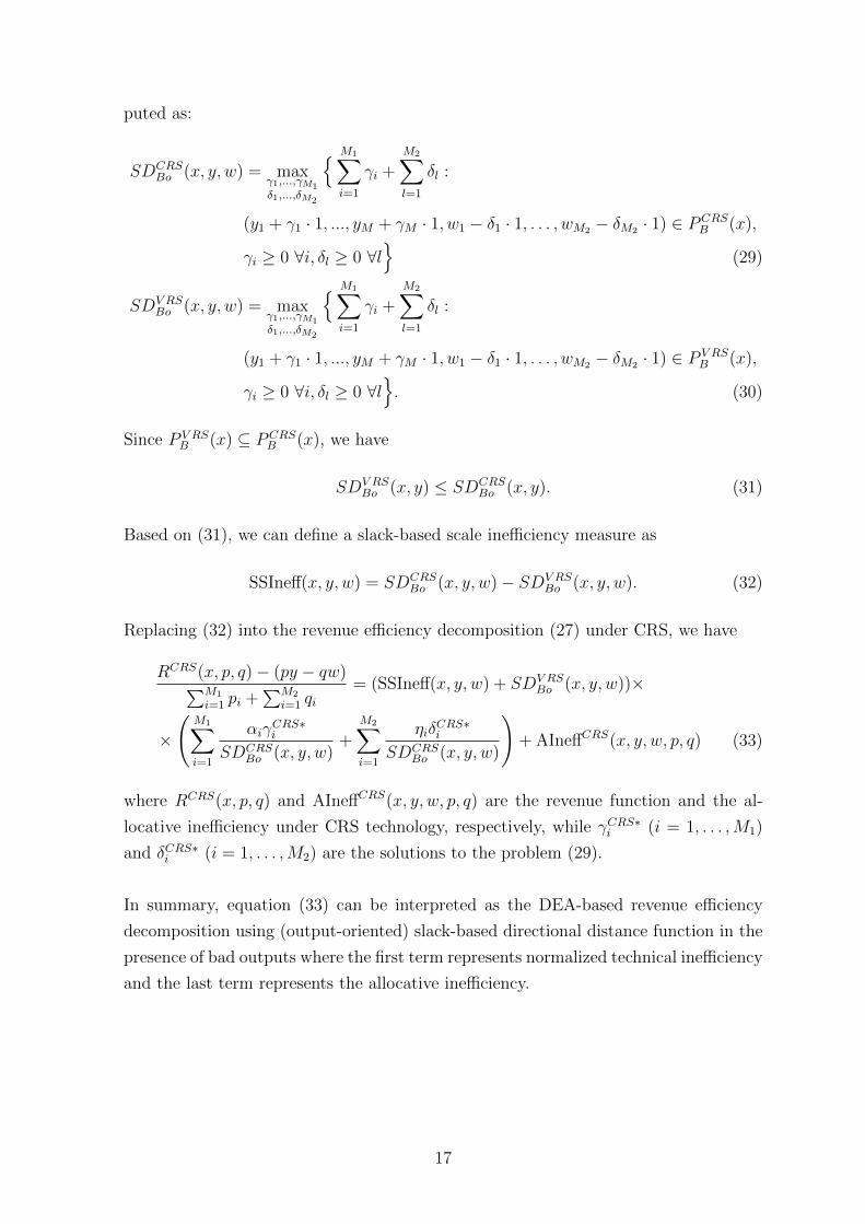
Equation (27) forms a decomposition of revenue e�ciency using the SD model where:

1.R(x, p, q)� (py � qw)P

M1

j=1 pj +P

M2

l=1 qlrepresents the normalized additive revenue e�ciency.

2. SDB

o

(x, y, w)⇥

P

M1

i=1

↵i

�⇤i

P

M1

j=1 �⇤j

+P

M2

l=1 �⇤l

+P

M2

t=1

⌘t

�⇤t

P

M1

j=1 �⇤j

+P

M2

l=1 �⇤l

!

represents

the normalized slack-based directional total technical ine�ciency term.

Subsequently, we introduce the framework for applying the above revenue decomposi-

tion to the DEA context. Similar to subsection 3.2, for x 2 RN

+ the reference technology

under CRS is:

PCRS

B

(x) =n

(y, w) 2 RM1 ⇥ RM2 :K

X

i=1

�kxk 5 x, ✓K

X

k=1

�kyk = y, ✓K

X

i=1

�kwk = w,

�k � 0 8k = 1, . . . , K, 0 ✓ 1o

(28)

and the reference technology under NIRS and VRS is obtained by adding the con-

straintsP

K

k=1 �k 1 and

P

K

k=1 �k = 1 to the right hand side of (28), respectively.

The output-oriented SD ine�ciency score in the presence of bad outputs can be com-

16

puted as:

SDCRS

Bo

(x, y, w) = max�1,...,�M1�1,...,�M2

n

M1X

i=1

�i

+M2X

l=1

�l

:

(y1 + �1 · 1, ..., yM + �M

· 1, w1 � �1 · 1, . . . , wM2 � �M2 · 1) 2 PCRS

B

(x),

�i

� 0 8i, �l

� 0 8lo

(29)

SDV RS

Bo

(x, y, w) = max�1,...,�M1�1,...,�M2

n

M1X

i=1

�i

+M2X

l=1

�l

:

(y1 + �1 · 1, ..., yM + �M

· 1, w1 � �1 · 1, . . . , wM2 � �M2 · 1) 2 P V RS

B

(x),

�i

� 0 8i, �l

� 0 8lo

. (30)

Since P V RS

B

(x) ✓ PCRS

B

(x), we have

SDV RS

Bo

(x, y) SDCRS

Bo

(x, y). (31)

Based on (31), we can define a slack-based scale ine�ciency measure as

SSIne↵(x, y, w) = SDCRS

Bo

(x, y, w)� SDV RS

Bo

(x, y, w). (32)

Replacing (32) into the revenue e�ciency decomposition (27) under CRS, we have

RCRS(x, p, q)� (py � qw)P

M1

i=1 pi +P

M2

i=1 qi= (SSIne↵(x, y, w) + SDV RS

Bo

(x, y, w))⇥

⇥

M1X

i=1

↵i

�CRS⇤i

SDCRS

Bo

(x, y, w)+

M2X

i=1

⌘i

�CRS⇤i

SDCRS

Bo

(x, y, w)

!

+AIne↵CRS(x, y, w, p, q) (33)

where RCRS(x, p, q) and AIne↵CRS(x, y, w, p, q) are the revenue function and the al-

locative ine�ciency under CRS technology, respectively, while �CRS⇤i

(i = 1, . . . ,M1)

and �CRS⇤i

(i = 1, . . . ,M2) are the solutions to the problem (29).

In summary, equation (33) can be interpreted as the DEA-based revenue e�ciency

decomposition using (output-oriented) slack-based directional distance function in the

presence of bad outputs where the first term represents normalized technical ine�ciency

and the last term represents the allocative ine�ciency.

17

5 Empirical application

The goal of this section is to provide an empirical illustration of the theoretical devel-

opments defined above when applying to a real data set.

5.1 Data sources

In this paper we use a data set on Vietnamese commercial banks which covers seven

years from 2008 to 2014. We constructed this data set by merging annual financial re-

ports that we downloaded for each individual bank wherever it was possible. The data

set includes 241 observations in total and is unbalanced because: (i) a small number

of banks did not publicly announce their financial reports, and (ii) a series of mergers

and acquisitions reduced the number of banks in the recent years.

We set a billion Vietnam Dong as the unit of measurement in our data set. Further-

more, after collecting raw data from financial reports, we smooth the seasonal e↵ects

by taking the averages of beginning- and end-year positions with regard to balance-

sheet items. Then, we use the GDP deflators (with 2010 as the base year) from World

Bank (2015) to adjust for the e↵ect of inflation.15 To ensure reasonably large number

of observations for DEA estimation, we pool the data over seven years.

5.2 Selection of inputs and outputs

It is admitted that measuring e�ciency in the banking industry is more di�cult than

in the manufacturing industries as there is no clear consensus on an appropriate identi-

fication of inputs and outputs (Sealey and Lindley, 1977). A simple logic mentioned in

Paradi and Zhu (2013) is that inputs are what banks would like to minimize and out-

puts are, conversely, what banks would like to maximize. Although adapting this logic,

we still see some components of financial statements which can be classified as either

inputs or outputs based on di↵erent viewpoints. An outstanding example is deposits

from customers. As Berger and Humphrey (1997) argued, on the one hand, banks have

to pay interests for deposits from customers and hence, they need to minimize deposits

to reduce interest burden. On the other hand, banks also need to enhance deposits in

order to have funds for making loans as well as gain bigger scale, which makes deposits

from customers possess the characteristics of both input and output at the same time.

In the banking industry, Kenjegalieva et al. (2009) summarized three popular ap-

proaches for selecting inputs and outputs which are the profit/revenue-based approach,

the production approach and the intermediation approach. A recent paper of Simper

15The base year of GDP deflators is 2010.

18

et al. (2015) also discussed di↵erent choices of inputs and outputs in banking industry.

In fact, the production approach which captures only physical inputs such as labor and

capital and their costs may be better for evaluating e�ciency at the branch level while

the intermediation approach, which also includes funds and interest costs, is considered

more appropriate for evaluation at the bank level (Berger and Humphrey, 1997). In

addition, while the intermediation approach counts some balance-sheet components as

outputs, only elements coming from income statements are considered as outputs in the

profit/revenue approach. There are also a wide variety of studies in which selections

of outputs and inputs do not follow a specific approach but mixed variations of them.

Moreover, the number of inputs and outputs in the model should not be neglected so

as to avoid the “curse of dimensionality” and ensure good separation and discrimina-

tion between decision-making-units (Paradi and Zhu, 2013). Assume that we have N

inputs, M outputs and K observations, there are some simple constraints suggested for

DEA to work properly. For instance, one common rule is K � 3(N +M) (see Jenkins

and Anderson, 2003) and another rule is K � max{NM, 3(N+M)} (see Cooper et al.,

2007).

Table 1: Description of input-output data (2008-2014) (241 observations)

Unit of measurement: Billion of Vietnam Dong

Mean Std. Dev. Min Max

Inputs

Operating expenses 1,360 2,177 21 14,210Fixed assets 867 1,089 29 5,459Deposits from customers 47,696 70,435 617 357,237Good outputs

Loans to customers net 43,319 71,439 327 391,080Securities 11,693 13,955 1 61,624Bad outputs

Provisions for credit losses of loans to customers 802 1,851 1 13,375

Notes: Balance-sheet items (Fixed assets, Deposits from customers, Loans to customers net,Securities, Provisions for credit losses of loans to customers) are calculated by taking the averageof the beginning- and end-year positions. Deflators corresponding to years from 2008 to 2014 usedto adjust data for inflation are 84, 89.2, 100, 121.3, 134.5, 140.9, 146.1, respectively (World Bank,2015).

Considering all points mentioned above, we follow the intermediation approach that

uses three inputs (operating expenses, fixed assets and deposits from customers), two

good outputs (net loans to customers, securities) and one bad output (provisions for

credit losses of loans to customers (PCL)). Two points should be highlighted here.

First, it is a common practice to select the number of employees as one type of inputs

in the intermediation approach. However, as this number as well as personnel expenses

are not always disclosed in published financial reports, we use operating expenses as

a proxy for the labor input in each bank. For the same reason, we employ PCL as

19

a proxy for NPLs. In essence, this is reasonable and does not a↵ect the reliability of

our results as banks are forced to make provisions for NPLs in accordance with laws

enacted by the government as discussed in section 4. A detailed description of these

inputs and outputs is shown in Table 1.

Since the goal of this paper is not about particular banks, we avoid finger-pointing

at bad or good banks by using the codes “B01”, “B02”, “B03”,..., “B40” to represent

individual banks, especially when providing qualitative information regarding some

specific banks in our case studies where relevant.

5.3 E�ciency of individual banks

Table 2 presents a summary on individual ine�ciency scores computed by di↵erent

measures (SD, DDF, HTE and TE) in the presence of bad outputs under di↵erent

types of returns to scale (CRS, NIRS and VRS). Box-plots of estimated ine�ciency

scores are also provided in Figure 3. Overall, we recognize some notable di↵erences in

ine�ciency scores computed by the four measures. First, although the SD and DDF

measure theoretically have the same range of values which is [0,+1), the observed

range of estimated ine�ciency scores computed by the SD measure (e.g., [0,69496] un-

der VRS) is remarkably larger than by the DDF measure (e.g., [0,517] under VRS).

This significant di↵erence stems from the fact that the DDF measure is a restricted

version of the SD measure as it does not allow the inputs and outputs to vary asym-

metrically but only allows a pre-specified direction. Second, the proportions of fully

e�cient banks estimated by the DDF, HTE and TE measures are higher than by the

SD measure, which is consistent with the theoretical result discussed in subsection 3.1.

Third, compared to the HTE and TE measures, the SD and DDF identify much more

outlying observations (Figure 3).16 Thus, a value added from SD relative to the other

measures is that it provides further hints on which banks need more detailed investiga-

tions to understand why their SD scores are extremely di↵erent from scores computed

by the other measures. Furthermore, the empirical evidence here also supports our

expectation that the SD measure help to di↵erentiate individual banks more than the

other measures.

Next, we investigate the correlations between rankings based on di↵erent e�ciency

measures by using the Spearman’s ⇢ statistic. As can be seen in Table 3, the rankings

based on the SD and DDF measures are highly correlated as their estimates of ⇢ are

about 0.87 under three types of returns to scale. In contrast, the ranking based on the

16Box-plots in Figure 3 are drawn using the default option in Matlab. To be precise, note that thebox-plots draw a point as outliers if it lies outside of the range [q1 � 1.5(q3 � q1), q3 + 1.5(q3 � q1)]where q1 and q3 are the 25th and 75th percentiles of the sample data, respectively.

20

SD measure is not well correlated with that based on the HTE and TE measures since

the corresponding correlation coe�cients are relatively low (between 0.35 and 0.54).

Table 2: Ine�ciency scores in the presence of bad outputs

DEA est. Mean Median Std. Dev. MaxFully e�cient banks

Quantity Proportion

CRS

SD 39,170 14,781 59,645 343,960 12 5%DDF 306 110 513 3,372 17 7%HTE 1.482 1.484 0.299 2.648 19 8%TE 1.499 1.479 0.307 2.881 17 7%

NIRS

SD 9,146 5,712 11,439 69,496 53 22%DDF 81 40 111 517 59 24%HTE 1.194 1.167 0.189 1.809 62 26%TE 1.235 1.203 0.228 2.036 59 24%

VRS

SD 9,113 5,712 11,403 69,496 56 23%DDF 81 40 111 517 61 25%HTE 1.190 1.160 0.189 1.809 64 27%TE 1.229 1.169 0.228 2.036 62 26%

Source: Authors’ calculations using Matlab.Non-linear optimization problems are solved by the “fmincon” solver with “sqp” option, incombination with “multistart” algorithm using 5 start points.

We also find that the ine�ciency scores are quite similar under VRS and NIRS. Re-

garding the SD measure, the maximum estimated ine�ciency scores under NIRS and

VRS are both 69496 with the most ine�cient bank being B35 in 2014 while under

CRS, the maximum estimated score is about five times larger (343960) with the most

ine�cient banks is B03 in 2012. For all measures, the correlation coe�cient of rank-

ings (Spearman’s ⇢ statistic) based on VRS and NIRS are extremely high (above 0.98)

whereas the ⇢ statistics corresponding to the pair CRS-VRS as well as CRS-NIRS are

relatively low (between 0.43 and 0.68) (Table 4).

Finally, as can be seen in Figure 4, estimated SD ine�ciency scores jumped up in

the period 2012-2014 on average, indicating a deterioration in bank e�ciency. Inter-

estingly, this jump is consistent with disadvantageous news that appeared in 2012, e.g.,

some bankers were suspected of illegal banking activities and arrested.17 In addition,

this figure also hints that the Scheme on “Restructuring the credit institutions sys-

tem in 2011-2015 period” did not bring back immediate positive e↵ects, in terms of

e�ciency of banks, as was expected.

17An arrest in August 2012 created a shock to the whole Vietnamese banking system, which waswell illustrated by dramatic falls of Vn-Index and HNX-Index, the benchmark indexes of stocks listedon two stock exchanges in Vietnam, in the next three consecutive days. Specifically, according toThomson Reuters Datastream, Vn-Index was down 4.7%, 1.6%, and 4.2% and HNX-Index was down5.2%, 3.4% and 5.3% on 21, 22 and 23 August 2012, respectively.

21

Figure 3: Box-plots of estimated ine�ciency scores

5.4 Remarks on some individual banks

In this subsection, we will investigate further the e�ciency of individual banks using

the SD ine�ciency scores computed under VRS. At the first glance, B39 is the only

bank having zero ine�ciency scores in six out of seven years. Following B39 is B04

which has five out of seven ine�ciency scores equal to zero. Thus, these two banks

can be considered the most e�cient banks in the period 2008-2014. Interestingly, they

are both large and state-owned.18 Conversely, B15, B35 and B08 can be viewed as the

most ine�cient banks because of their remarkably large ine�ciency scores. While B08

and B15 are of medium banks, B35 is in the group of the four largest banks.

18In this paper, we divide banks into three categories based on total assets: (i) large banks - thefour largest banks, (ii) medium banks - the twelve largest banks, excluding banks in group (i), and(iii) small banks - the remaining banks.

22

Table 3: Correlation of ranks (Spearman’s ⇢ statistic)

SD DDF HTE TE

CRS

SD 1.000 0.871 0.367 0.353DDF 1.000 0.406 0.366HTE 1.000 0.923TE 1.000

NIRS

SD 1.000 0.866 0.485 0.510DDF 1.000 0.597 0.595HTE 1.000 0.980TE 1.000

VRS

SD 1.000 0.866 0.508 0.535DDF 1.000 0.616 0.618HTE 1.000 0.980TE 1.000

Source: Authors’ calculations.

Table 4: Correlations of rankings (Spearman’s ⇢) under di↵erent returns to scale

CRS NIRS VRS

SDCRS 1.000 0.430 0.438NIRS 1.000 0.999VRS 1.000

DDFCRS 1.000 0.447 0.453NIRS 1.000 0.999VRS 1.000

HTECRS 1.000 0.611 0.633NIRS 1.000 0.992VRS 1.000

TECRS 1.000 0.660 0.681NIRS 1.000 0.988VRS 1.000

Source: Authors’ calculations.

We also observe several banks showing deterioration in e�ciency as their ranks are

downgraded through years, e.g., B02 (from 1 to 232), B13 (from 63 to 163), B17 (from

1 to 170), B30 (from 121 to 215), B36 (from 1 to 142).19 On the contrary, B32, a

medium bank, demonstrates an admirable improvement in e�ciency as its rank climbs

from 231 (in 2009) to 1 (in 2014). Overall, we see that deteriorating banks outnum-

bered the improving banks.

Looking at the ine�ciency scores in more details, we see that 30% of fully e�cient

banks estimated by the SD under VRS are state-owned while the proportion of this

type of ownership only accounts for 14% in the whole data set, suggesting that state-

owned banks operate more e�cient than the others. Similarly, although small banks

19Rank 1 means the most e�cient bank.

23

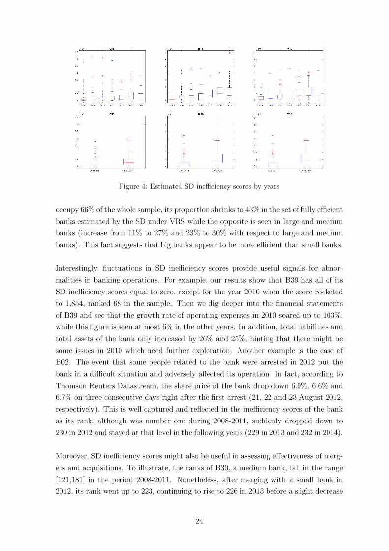
Figure 4: Estimated SD ine�ciency scores by years

occupy 66% of the whole sample, its proportion shrinks to 43% in the set of fully e�cient

banks estimated by the SD under VRS while the opposite is seen in large and medium

banks (increase from 11% to 27% and 23% to 30% with respect to large and medium

banks). This fact suggests that big banks appear to be more e�cient than small banks.

Interestingly, fluctuations in SD ine�ciency scores provide useful signals for abnor-

malities in banking operations. For example, our results show that B39 has all of its

SD ine�ciency scores equal to zero, except for the year 2010 when the score rocketed

to 1,854, ranked 68 in the sample. Then we dig deeper into the financial statements

of B39 and see that the growth rate of operating expenses in 2010 soared up to 103%,

while this figure is seen at most 6% in the other years. In addition, total liabilities and

total assets of the bank only increased by 26% and 25%, hinting that there might be

some issues in 2010 which need further exploration. Another example is the case of

B02. The event that some people related to the bank were arrested in 2012 put the

bank in a di�cult situation and adversely a↵ected its operation. In fact, according to

Thomson Reuters Datastream, the share price of the bank drop down 6.9%, 6.6% and

6.7% on three consecutive days right after the first arrest (21, 22 and 23 August 2012,

respectively). This is well captured and reflected in the ine�ciency scores of the bank

as its rank, although was number one during 2008-2011, suddenly dropped down to

230 in 2012 and stayed at that level in the following years (229 in 2013 and 232 in 2014).

Moreover, SD ine�ciency scores might also be useful in assessing e↵ectiveness of merg-

ers and acquisitions. To illustrate, the ranks of B30, a medium bank, fall in the range

[121,181] in the period 2008-2011. Nonetheless, after merging with a small bank in

2012, its rank went up to 223, continuing to rise to 226 in 2013 before a slight decrease

24

to 215 in 2014. We then investigate the financial statements of B30 and see that this

bank had to make provisions for credit losses of loans belonging to its merger partner,

resulting in a significant reduction in its annual profits. Therefore, changing in the SD-

based ranks of the bank appears to be consistent with the bank’s operation in reality.

Presented evidence support our expectation that SD ine�ciency score can be a useful

indicator for analyzing the performance of banks in general. To understand perfor-

mance of individual banks in more details with comprehensive explanations, one could

then conduct deeper case studies which are beyond the scope of this paper.

5.5 Analysis of e�ciency distributions

In this subsection, we analyze the distributions of ine�ciency scores using kernel den-

sity estimation and related tests. Our procedure is adapted from the framework con-

structed for the Farrell-type technical e�ciency which was proposed by Simar and

Zelenyuk (2006), who in turn adapted the approach of Li (1996, 1999).

First, we do kernel density estimations of ine�ciency scores under CRS, NIRS and

VRS (Figure 5). Two crucial points are: (i) We overcome the issue of bounded support

in density estimation by employing the reflection method proposed by Schuster (1985)-

Silverman (1986) (for details, see Simar and Zelenyuk, 2006), and (ii) To calculate the

bandwidths, we use the Sheather and Jones’s (1991) method.20 As can be seen in Fig-

ure 5, DDF, HTE and TE ine�ciency scores follow patterns which are di↵erent with

that of the SD ine�ciency scores. The SD has wide estimated ranges of values and

long tails compared to the other measures. In addition, the estimated densities under

NIRS and VRS look similar whereas being di↵erent with those under CRS. In Figure

5 we also show kernel density estimations of ine�ciency scores in the period 2008-2011

and 2012-2014. In all cases, the densities corresponding to period 2008-2011 lie above

those corresponding to the period 2012-2014 to the left, suggesting that in 2008-2011

banks operated more e�ciently than in 2012-2014.

Figure 6 presents the kernel densities estimations contrasting the di↵erent types of

ownership (state-owned versus non-state-owned) and bank sizes (large, medium and

small). Interestingly, state-owned banks are apparently more e�cient than non-state-

owned banks by the SD and DDF measures while the opposite is seen by the HTE

and TE measures. Analogously, SD and DDF measures recognise large banks as more

e�cient than small banks while the kernel density estimations corresponding to the

HTE and TE measure show the opposite.

20Theoretically, SD and DDF ine�ciency scores are bounded below by 0 while HTE and TE ine�-ciency scores are bounded below by 1.

25

Figure 5: Estimated densities of DEA-estimated ine�ciency scores using Sheather and Jones’s(1991) bandwidth: Period 2008-2014 and two subperiods 2008-2011 and 2012-2014

Subsequently, we perform tests for equality of densities (adapted from Li, 1996, 1999;

Simar and Zelenyuk, 2006) to see whether statistical evidences support the conclusions

which we have drawn from kernel density estimations. This aim can be hypothesized

as8

<

:

H0 : fA(u) = fZ

(u) for all u in the relevant support

H1 : fA(u) 6= fZ

(u) on a set of positive measures

where A and Z are two types of ine�ciency scores which we are going to examine and

fA

and fZ

denote their density functions, respectively.

For conducting these tests, we adapt the Algorithm II from Simar and Zelenyuk (2006)

26

Figure 6: Estimated densities of DEA-estimated ine�ciency scores using Sheather and Jones’s(1991) bandwidth: State-ownership and bank sizes

Table 5: Adapted Li (1996) test for equality of densities of the DDF and SD ine�ciencyscores

Returns to scale Li test statistic Reject H0

CRS 94.9897 [0.000] YesVRS 43.2422 [0.000] YesNIRS 45.7596 [0.000] Yes

Source: Authors’ calculations using Matlab.Bootstrapped p-values are provided in brackets. De-cisions on rejecting H0 are based on 5% level of signif-icance.

with 2000 bootstrap replications and Silverman’s (1986) rule-of-thumb bandwidth com-

27

Table 6: Adapted Li (1996) test for equality of densities under di↵erent returns to scale

Li test statistic Reject H0

SDCRS vs VRS 13.7053 [0.0000] YesCRS vs NIRS 13.6615 [0.0000] YesVRS vs NIRS 0.0060 [0.9955] No

DDFCRS vs VRS 11.0927 [0.0000] YesCRS vs NIRS 11.0466 [0.0000] YesVRS vs NIRS 0.0019 [0.9970] No

HTECRS vs VRS 35.0441 [0.0000] YesCRS vs NIRS 33.5435 [0.0000] YesVRS vs NIRS 0.0581 [0.9440] No

TECRS vs VRS 30.4120 [0.0000] YesCRS vs NIRS 28.4234 [0.0000] YesVRS vs NIRS 0.0738 [0.9260] No

Source: Authors’ calculations using Matlab.Bootstrapped p-values are provided in brackets. Decisionson rejecting H0 are based on 5% level of significance.

Table 7: Adapted Li (1996) test for equality of densities of estimated ine�ciency scores bydi↵erent time periods and ownership

Measures Returns to scale2008-2011 vs. 2012-2014

State-owned vs.Non-state-owned

SDCRS 6.3382 [0.0000] 14.0446 [0.0000]VRS 8.1510 [0.0000] 6.1749 [0.0000]NIRS 8.3161 [0.0000] 6.3671 [0.0000]

DDFCRS 6.2004 [0.0000] 16.4047 [0.0000]VRS 9.5654 [0.0000] 3.7819 [0.0005]NIRS 9.6411 [0.0000] 3.8626 [0.0010]

HTECRS 5.0077 [0.0000] 1.6149 [0.0275]VRS 0.8959 [0.1160]n 5.7069 [0.0000]NIRS 0.7248 [0.2950]n 6.2554 [0.0000]

TECRS 2.9188 [0.0070] 3.2836 [0.0030]VRS 0.1538 [0.8365]n 6.1958 [0.0000]NIRS -0.0413 [0.9610]n 6.7491 [0.0000]

Source: Authors’ calculations using Matlab.Bootstrapped p-values are provided in brackets beside Li test statistics. Decisionson rejecting H0 are based on 5% level of significance. n Do not reject H0.

puted in each bootstrap iteration.21 Table 5 reports results of comparing the SD and

DDF ine�ciency scores. Based on the bootstrapped p-values, we can reject the null

hypothesis of identical densities under all types of returns to scale at 95% level of con-

fidence. In addition, as reported in Table 6, for all types of measures, the densities of

ine�ciency scores under VRS and NIRS are similar but they are not identical to the

21A common practice is to calculate the Silverman’s (1986) rule-of-thumb bandwidth as h =

1.06n�1/5 min{�(✏), iqr(✏)1.349 } where n is the sample size, �(✏) and iqr(✏) are the estimated standard

deviation and interquartile range for the variable of interest ✏, respectively.

28

density under CRS at 5% level of significance. For the sake of completeness, we also

compare densities of estimated ine�ciency scores of di↵erent groups using the adapted

Li (1996) tests: (i) period 2008-2012 versus 2012-2014 and (ii) state-owned versus non-

state-owned banks. All in all, the evidence from the adapted Li (1996) test is generally

consistent with our kernel density estimations and analyses in subsection 5.3.

6 Concluding remarks

The first and main goal of this paper is to extend the slack-based directional distance

function to the context of measuring e�ciency in the presence of bad outputs. The

second goal of this paper was to use the SD measure to propose decompositions of

revenue e�ciency in the presence of bad outputs, which is a further extension of Fare

et al. (2005). In essence, our decompositions separate the normalized SD-based revenue

e�ciency as a sum of two components: (i) the normalized technical ine�ciency and

(ii) the allocative ine�ciency. It is also worth noting that the revenue decompositions

proposed in this paper are applicable to not only the banking industry but also a num-

ber of other production processes.

The third goal of this paper was to illustrate our theoretical developments by ap-

plying the SD to measure the e�ciency of Vietnamese commercial banks. In doing

so, we find that SD measure helps discriminate individual banks more relative to the

DDF, HTE and TE measure. We also find that fluctuations in SD ine�ciency scores

seem to go closely with operations and performances of banks and also consist with

fundamental analyses based on financial reports. We discover that ine�ciency scores

under VRS and NIRS are quite similar whereas they are significantly di↵erent with

those under CRS.

Using the SD ine�ciency scores, we find some characteristics of Vietnamese commer-

cial banks which might be helpful to policy-makers. First, banks in period 2012-2014

are generally less e�cient when compared to the period 2008-2011. Second, large

banks appear to be more e�cient than the others and so do state-owned banks. Bank

regulators can benefit from using rankings of banks based on ine�ciency scores to

identify ine�cient banks or groups of banks to focus on in their regulation and re-

structuring the Vietnamese banking system. To some extent, the increase in estimated

ine�ciency scores in 2012-2014 might suggest SBV to consider carefully its Scheme on

“Restructuring the credit institutions system in the 2011-2015 period” for appropriate

improvements in future schemes.

This paper also suggests some directions for future research. First, while our analysis in

29

this paper focuses on using the SD to measure e�ciency of banks in the presence of bad

outputs, a natural future expansion is to regress the estimated SD ine�ciency scores

on hypothesized factors which might have potential impacts on bank e�ciency.22 In

particular, it is promising to generalize the truncated regression and double bootstrap

approach which was originally developed for the Farrell-type measure in the standard

DEA context by Simar and Wilson (2007). The second direction would be to adapt

the most recent theories from Kneip et al. (2015, 2016) to empower statistical analysis

using SD-type measures. Last but not least, it is also interesting to develop the the-

ory of aggregation of ine�ciency scores based on the SD measure, which is useful in

analyzing e�ciency of groups of banks sharing a common property, e.g., ownership or

size.

Acknowledgements

We would like to thank the Editor, three anonymous referees and participants of various

workshops where this paper was presented for their valuable feedback. We also thank

Alexander Cameron for English proofreading.

22We also thank an anonymous referee for suggesting a second-stage analysis with regards to theSD measure.

30

Appendix A

Here we confirm that removing ✓ from the problem (15) does not change the optimal

value of the objective function when computing SD ine�ciency scores under NIRS.

The proofs for CRS and the other measures are similar.

Assume that (�⇤1 , . . . , �

⇤N

, �⇤1 , . . . , �

⇤M1

, �⇤1, . . . , �⇤M2

,�1⇤, . . . ,�K⇤, ✓⇤) is a solution the prob-

lem (15) under NIRS:

max�1,...,�N ,�1,...,�M1

�1,...,�M2 ,�1,...,�

K,✓

N

X

i=1

�i

+M1X

j=1

�j

+M2X

l=1

�l

!

(15)

subject to:

xo

i

� �i

�P

K

k=1 �kxk

i

8i = 1, . . . , N

yoj

+ �j

✓P

K

k=1 �kyk

j

8j = 1, . . . ,M1

wo

l

� �l

= ✓P

K

k=1 �kwk

l

8l = 1, . . . ,M2

�k � 0 8k = 1, . . . , K; �i

� 0 8i = 1, . . . , N

�j

� 0 8j = 1, . . . ,M1; �l � 0 8l = 1, . . . ,M2P

K

k=1 �k 1; 0 ✓ 1

and (�1, . . . , �N

, �1, . . . , �M1 , �1, . . . , �M2 , �1, . . . , �K) is a solution of

max�1,...,�N ,�1,...,�M1

�1,...,�M2 ,�1,...,�

K

N

X

i=1

�i

+M1X

j=1

�j

+M2X

l=1

�l

!

(34)

subject to:

xo

i

� �i

�P

K

k=1 �kxk

i

8i = 1, . . . , N

yoj

+ �j

P

K

k=1 �kyk

j

8j = 1, . . . ,M1

wo

l

� �l

=P

K

k=1 �kwk

l

8l = 1, . . . ,M2

�k � 0 8k = 1, . . . , K; �i

� 0 8i = 1, . . . , N

�j

� 0 8j = 1, . . . ,M1; �l � 0 8l = 1, . . . ,M2P

K

k=1 �k 1

then we need to prove thatP

N

i=1 �⇤i

+P

M1

j=1 �⇤j

+P

M2

l=1 �⇤l

=P

N

i=1 �i

+P

M1

j=1 �j+P

M2

l=1 �l.

Firstly, it is transparent that (�1, . . . , �N

, �1, . . . , �M1 , �1, . . . , �M2 , �1, . . . , �K , 1) satisfies

constraints of problem (15). Thus,

N

X

i=1

�⇤i

+M1X

j=1

�⇤j

+M2X

l=1

�⇤l

�N

X

i=1

�i

+M1X

j=1

�j

+M2X

l=1

�l

(35)

31

Secondly, since 0 ✓⇤ 1, we have

xo

i

� �⇤i

�K

X

k=1

�k⇤xk

i

�K

X

k=1

(✓⇤�k⇤)xk

i

8i = 1, . . . , N

and

K

X

k=1

(✓⇤�k⇤) K

X

k=1

�k⇤ 1

Hence, it is clear that (�⇤1 , . . . , �

⇤N

, �⇤1 , . . . , �

⇤M

, �⇤1, . . . , �⇤M2

, ✓⇤�1⇤, . . . , ✓⇤�K⇤) satisfies

constraints of problem (34). As a consequence,

N

X

i=1

�⇤i

+M1X

j=1

�⇤j

+M2X

l=1

�⇤l

N

X

i=1

�i

+M1X

j=1

�j

+M2X

l=1

�l

(36)

From (35) and (36), we have the desired result.

32

Appendix B Summary of ine�ciency scores

Table A1: Average of ine�ciency scores: SD and DDF

BanksCRS NIRS VRSSD DDF SD DDF SD DDF

B01 19,660 210 13,183 172 13,183 172B02 88,893 562 16,054 154 16,054 154B03 305,652 2,566 15,823 0 15,273 0B04 134,353 802 7,584 76 7,584 76B05 4,128 17 3,987 17 3,832 16B06 3,038 32 2,852 31 2,582 30B07 3,726 27 3,275 22 3,177 22B08 31,581 356 16,119 193 16,119 193B09 35,348 338 9,105 74 9,105 74B10 8,408 28 5,693 22 5,693 22B11 7,383 87 3,111 64 3,111 64B12 17,280 100 8,402 61 8,402 61B13 5,985 49 5,003 46 4,912 45B14 19,644 137 8,028 76 8,028 76B15 65,022 610 26,163 296 26,163 296B16 1,301 8 1,298 7 1,105 6B17 10,554 171 5,755 86 5,755 86B18 32,786 221 6,059 55 6,059 55B19 5,637 33 4,800 31 4,796 31B20 16,990 44 5,588 21 5,588 21B21 10,309 68 7,894 60 7,894 60B22 7,061 108 5,206 77 5,206 77B23 20,338 46 11,558 21 11,558 21B24 6,755 78 5,799 68 5,752 67B25 14,435 70 6,537 53 6,537 53B26 20,704 136 9,390 116 9,390 116B27 16,624 97 6,159 56 6,159 56B28 26,659 225 7,547 116 7,547 116B29 7,331 82 6,067 75 6,067 75B30 31,532 254 16,153 191 16,153 191B31 71,971 566 22,547 191 22,547 191B32 71,053 460 13,697 82 13,697 82B33 0 0 0 0 0 0B34 6,929 76 4,739 66 4,739 66B35 180,032 990 41,142 248 41,142 248B36 3,482 32 2,996 30 2,940 30B37 21,528 113 4,399 42 4,399 42B38 22,773 128 3,840 18 3,840 18B39 137,740 1,689 265 2 265 2B40 4,964 17 4,315 17 4,279 17

33

Table A2: Average of ine�ciency scores: HTE and TE

BanksCRS NIRS VRS

HTE TE HTE TE HTE TEB01 1.908 1.882 1.487 1.587 1.487 1.587B02 1.797 1.847 1.090 1.116 1.090 1.116B03 1.257 1.267 1.000 1.000 1.000 1.000B04 1.137 1.138 1.014 1.015 1.014 1.015B05 1.468 1.575 1.447 1.560 1.442 1.467B06 1.308 1.348 1.277 1.334 1.240 1.292B07 1.282 1.338 1.221 1.291 1.188 1.271B08 1.594 1.604 1.151 1.181 1.151 1.181B09 1.484 1.509 1.093 1.123 1.093 1.123B10 1.666 1.722 1.359 1.459 1.359 1.459B11 1.254 1.215 1.148 1.151 1.148 1.151B12 1.586 1.589 1.207 1.276 1.207 1.276B13 1.553 1.617 1.394 1.506 1.377 1.485B14 1.452 1.451 1.178 1.198 1.178 1.198B15 2.014 1.936 1.313 1.367 1.313 1.367B16 1.250 1.280 1.247 1.278 1.210 1.235B17 1.383 1.365 1.141 1.162 1.141 1.162B18 1.536 1.529 1.067 1.082 1.067 1.082B19 1.522 1.571 1.392 1.470 1.392 1.469B20 1.275 1.264 1.060 1.078 1.060 1.078B21 1.568 1.609 1.329 1.400 1.329 1.400B22 1.400 1.400 1.227 1.240 1.227 1.240B23 1.494 1.383 1.077 1.092 1.077 1.092B24 1.486 1.481 1.361 1.398 1.349 1.385B25 1.274 1.336 1.133 1.172 1.133 1.172B26 1.458 1.413 1.186 1.196 1.186 1.196B27 1.526 1.450 1.193 1.198 1.193 1.198B28 1.247 1.242 1.038 1.059 1.038 1.059B29 1.535 1.551 1.364 1.419 1.364 1.419B30 1.617 1.654 1.262 1.350 1.262 1.350B31 1.540 1.845 1.090 1.170 1.090 1.170B32 1.911 1.897 1.107 1.159 1.107 1.159B33 1.000 1.000 1.000 1.000 1.000 1.000B34 1.367 1.366 1.238 1.270 1.238 1.270B35 1.513 1.458 1.068 1.076 1.068 1.076B36 1.371 1.363 1.282 1.326 1.271 1.313B37 1.364 1.334 1.060 1.068 1.060 1.068B38 1.468 1.500 1.044 1.058 1.044 1.058B39 1.265 1.391 1.000 1.000 1.000 1.000B40 1.630 1.750 1.490 1.622 1.462 1.596

34

References

Berger, A. N. and Humphrey, D. B. (1997). E�ciency of Financial Institutions: Inter-

national Survey and Directions for Future Research. European Journal of Operational

Research, 98(2):175–212.

Berger, A. N. and Mester, L. J. (2003). Explaining the dramatic changes in perfor-

mance of US banks: technological change, deregulation, and dynamic changes in

competition. Journal of Financial Intermediation, 12(1):57–95.

Chambers, R., Chung, Y., and Fare, R. (1998). Profit, Directional Distance Func-

tions, and Nerlovian E�ciency. Journal of Optimization Theory and Applications,

98(2):351–364.

Chambers, R. G., Chung, Y., and Fare, R. (1996). Benefit and distance functions.

Journal of Economic Theory, 70(2):407–419.

Charnes, A., Cooper, W., Golany, B., Seiford, L., and Stutz, J. (1985). Foundations

of data envelopment analysis for Pareto-Koopmans e�cient empirical production

functions. Journal of Econometrics, 30(1-2):91–107.

Chung, Y., Fare, R., and Grosskopf, S. (1997). Productivity and Undesirable Outputs:

A Directional Distance Function Approach. Journal of Environmental Management,

51(3):229–240.

Cooper, W. W., Seiford, L. M., and Tone, K. (2007). Data Envelopment Analysis:

A Comprehensive Text with Models, Applications, References and DEA-Solver Soft-

ware. Springer, New York.

Curi, C., Lozano-Vivas, A., and Zelenyuk, V. (2015). Foreign bank diversification and

e�ciency prior to and during the financial crisis: Does one business model fit all?

Journal of Banking & Finance, 61:S22–S35.

Du, K., Worthington, A. C., and Zelenyuk, V. (2015). The dynamic relationship

between bank asset diversification and e�ciency: Evidence from the Chinese banking

sector. Centre for E�ciency and Productivity Analysis Working Paper Series No.

WP12/2015.

Fare, R., Fukuyama, H., Grosskopf, S., and Zelenyuk, V. (2015). Decomposing profit

e�ciency using a slack-based directional distance function. European Journal of

Operational Research, 247(1):335–337.

Fare, R., Fukuyama, H., Grosskopf, S., and Zelenyuk, V. (2016). Cost decompositions

and the e�cient subset. Omega, 62:123–130.

35

Fare, R. and Grosskopf, S. (2003). Nonparametric Productivity Analysis with Undesir-

able Outputs: Comment. American Journal of Agricultural Economics, 85(4):1070–

1074.

Fare, R. and Grosskopf, S. (2009). A Comment on Weak Disposability in Nonparamet-

ric Production Analysis. American Journal of Agricultural Economics, 91(2):535–

538.

Fare, R. and Grosskopf, S. (2010). Directional distance functions and slacks-based

measures of e�ciency. European Journal of Operational Research, 200(1):320–322.

Fare, R., Grosskopf, S., and Lovell, C. A. K. (1994). Production frontiers. Cambridge

University Press.

Fare, R., Grosskopf, S., Lovell, C. A. K., and Pasurka, C. (1989). Multilateral Pro-

ductivity Comparisons When Some Outputs are Undesirable: A Nonparametric Ap-

proach. The Review of Economics and Statistics, 71(1):90.

Fare, R., Grosskopf, S., Noh, D.-W., and Weber, W. (2005). Characteristics of a

polluting technology: theory and practice. Journal of Econometrics, 126(2):469–

492.

Fare, R. and Lovell, C. (1978). Measuring the technical e�ciency of production. Journal

of Economic Theory, 19(1):150–162.

Fare, R. and Primont, D. (1995). Multi-Output Production and Duality: Theory and

Applications. Springer Netherlands, Dordrecht.

Farrell, M. J. (1957). The Measurement of Productive E�ciency. Journal of the Royal

Statistical Society. Series A, 120(3):253–290.

Fethi, M. D. and Pasiouras, F. (2010). Assessing bank e�ciency and performance

with operational research and artificial intelligence techniques: A survey. European

Journal of Operational Research, 204(2):189–198.

Fletcher, R. (1987). Practical Methods of Optimization. Wiley.

Fukuyama, H. andWeber, W. L. (2009). A directional slacks-based measure of technical

ine�ciency. Socio-Economic Planning Sciences, 43(4):274–287.

Fukuyama, H. and Weber, W. L. (2010). A slacks-based ine�ciency measure for a

two-stage system with bad outputs. Omega, 38(5):398–409.

Gill, P. E., Murray, W., and Wright, M. H. (1981). Practical Optimization. Academic

Press, Practical Optimization.

36

Han, S. P. (1977). A globally convergent method for nonlinear programming. Journal

of Optimization Theory and Applications, 22(3):297–309.

Hock, W. and Schittkowski, K. (1983). A comparative performance evaluation of 27

nonlinear programming codes. Computing, 30(4):335–358.

Jenkins, L. and Anderson, M. (2003). A multivariate statistical approach to reducing

the number of variables in data envelopment analysis. European Journal of Opera-

tional Research, 147(1):51–61.

Kenjegalieva, K., Simper, R., Weyman-Jones, T., and Zelenyuk, V. (2009). Com-

parative analysis of banking production frameworks in eastern european financial

markets. European Journal of Operational Research, 198(1):326–340.

Kneip, A., Simar, L., and Wilson, P. W. (2015). When bias kills the variance: Central

limit theorems for dea and fdh e�ciency scores. Econometric Theory, 31(2):394–422.

Kneip, A., Simar, L., and Wilson, P. W. (2016). Testing hypotheses in nonparametric

models of production. Journal of Business & Economic Statistics, 34(3):435–456.

Kuosmanen, T. (2005). Weak Disposability in Nonparametric Production Analysis with

Undesirable Outputs. American Journal of Agricultural Economics, 87(4):1077–1082.

Kuosmanen, T. and Podinovski, V. (2009). Weak Disposability in Nonparametric

Production Analysis: Reply to Fare and Grosskopf. American Journal of Agricultural

Economics, 91(2):539–545.

Li, Q. (1996). Nonparametric testing of closeness between two unknown distribution

functions. Econometric Reviews, 15(3):261–274.

Li, Q. (1999). Nonparametric testing the similarity of two unknown density func-

tions: local power and bootstrap analysis. Journal of Nonparametric Statistics,

11(1-3):189–213.

Lozano, S. (2016). Slacks-based ine�ciency approach for general networks with bad

outputs: An application to the banking sector. Omega, 60:73–84.

Paradi, J. C. and Zhu, H. (2013). A survey on bank branch e�ciency and performance

research with data envelopment analysis. Omega, 41:61–79.

Park, K. H. and Weber, W. L. (2006). A note on e�ciency and productivity growth in

the Korean Banking Industry, 1992-2002. Journal of Banking & Finance, 30(8):2371–

2386.

37

Portela, M. C. A. S., Thanassoulis, E., and Simpson, G. (2004). Negative data in DEA:

a directional distance approach applied to bank branches. Journal of the Operational

Research Society, 55(10):1111–1121.

Powell, M. J. D. (1978a). A fast algorithm for nonlinearly constrained optimization

calculations. Lecture Notes in Mathematics-Numerical Analysis, 630:144–157.

Powell, M. J. D. (1978b). Nonlinear Programming 3, chapter The Convergence of

Variable Metric Methods For Nonlinearly Constrained Optimization Calculations.

Academic Press.

Ratcli↵e, S. (2011). Oxford Treasury of Sayings and Quotations. Oxford University

Press, 4 edition.

Schuster, E. F. (1985). Incorporating support constraints into nonparametric estima-

tors of densities. Communications in Statistics - Theory and Methods, 14(5):1123–

1136.

Sealey, C. W. J. and Lindley, J. T. (1977). Inputs, outputs, and a theory of production

and cost at depository financial institutions. The Journal of Finance, 32(4):1251–

1266.

Seiford, L. M. and Zhu, J. (2002). Modeling undesirable factors in e�ciency evaluation.

European Journal of Operational Research, 142(1):16–20.

Sheather, S. J. and Jones, M. C. (1991). A reliable data-based bandwidth selection

method for kernel density estimation. Journal of the Royal Statistical Society. Series

B, 53(3):683–690.

Silverman, B. W. (1986). Density Estimation for Statistics and Data Analysis. Chap-

man and Hall, London.

Simar, L. and Wilson, P. W. (2007). Estimation and inference in two-stage, semi-

parametric models of production processes. Journal of Econometrics, 136(1):31–64.

Simar, L. and Zelenyuk, V. (2006). On Testing Equality of Distributions of Technical

E�ciency Scores. Econometric Reviews, 25(4):497–522.

Simper, R., Hall, M. J. B., Liu, W., Zelenyuk, V., and Zhou, Z. (2015). How relevant

is the choice of risk management control variable to non-parametric bank profit

e�ciency analysis? The case of South Korean banks. Annals of Operations Research.

The State Bank of Vietnam (2008). Annual report 2008.

The State Bank of Vietnam (2009). Annual report 2009.

38

The State Bank of Vietnam (2010). Annual report 2010.

The State Bank of Vietnam (2011). Annual report 2011.

The State Bank of Vietnam (2012). Annual report 2012.

The State Bank of Vietnam (2013). Annual report 2013.

The State Bank of Vietnam (2014). Annual report 2014.

The State Bank of Vietnam (2016a). History of Vietnamese banks 1951-2016. Labour

Publishing House (Vietnam), Hanoi.

The State Bank of Vietnam (2016b). System of Credit Institutions.

Tone, K. (2001). A slacks-based measure of e�ciency in data envelopment analysis.

European Journal of Operational Research, 130(3):498–509.

World Bank (2015). World Bank Open Data.

Zelenyuk, N. and Zelenyuk, V. (2015). Drivers of E�ciency in Banking: Importance

of Model Specifications. Centre for E�ciency and Productivity Analysis Working

Paper Series No. WP08/2015.

39

Supplement

Table S1: SD ine�ciency scores under CRS

Banks Year2008 2009 2010 2011 2012 2013 2014

B01 6,063 12,203 19,925 17,974 21,324 28,414 31,717B02 80,178 79,792 73,038 92,047 102,585 94,073 100,540B03 277,656 307,816 308,503 290,324 343,960B04 136,175 140,802 175,755 155,994 0 150,471 181,273B05 3,040 4,834 4,510B06 1,349 3,543 3,840 2,514 3,944B07 888 3,516 4,565 5,933B08 19,845 24,830 24,407 24,288 30,699 43,682 53,317B09 31,265 36,640 29,426 21,279 29,965 45,097 53,762B10 6,466 10,350B11 8,156 9,486 7,355 4,534B12 0 6,274 8,960 10,283 18,360 33,916 43,170B13 1,322 3,204 4,791 5,289 7,219 9,008 11,059B14 3,348 0 9,733 25,379 36,587 42,814B15 30,828 38,506 52,005 67,411 82,545 85,942 97,918B16 518 368 3,912 3,610 0 565 134B17 1,341 4,134 9,343 11,415 14,591 16,004 17,049B18 11,514 20,380 29,630 34,847 42,902 46,781 43,449B19 3,699 3,890 3,984 3,724 5,427 7,459 11,276B20 12,386 22,930 15,654B21 8,205 7,648 7,884 9,644 9,310 12,369 17,103B22 5,986 6,775 6,487 4,500 5,691 9,119 10,868B23 0 11,802 27,123 29,944 27,186 25,973B24 868 4,491 7,863 7,871 7,918 8,090 10,185B25 10,984 7,538 8,261 18,340 27,054B26 0 41,408B27 6,181 10,646 10,874 17,006 25,351 23,093 23,219B28 17,531 14,781 20,358 44,104 63,177 0B29 7,129 7,906 7,509 6,174 7,061 7,995 7,542B30 7,166 13,513 17,789 22,131 46,171 61,041 52,914B31 53,544 60,529 58,454 56,669 69,616 94,724 110,259B32 74,516 69,191 57,820 65,788 78,779 80,225B33 0 0 0 0B34 6,679 9,467 6,598 2,084 5,928 10,159 7,586B35 149,928 176,849 180,810 172,690 172,070 187,279 220,596B36 0 380 1,224 1,122 4,783 8,309 8,556B37 20,965 28,355 23,302 15,846 20,076 21,508 20,643B38 14,987 17,147 12,459 8,819 24,647 40,987 40,366B39 109,193 96,604 125,640 127,522 134,958 170,687 199,578B40 587 1,969 4,004 8,207 10,054

40

Table S2: SD ine�ciency scores under NIRS

Banks Year2008 2009 2010 2011 2012 2013 2014

B01 5,202 8,930 12,246 11,947 15,483 19,038 19,432B02 0 0 0 0 37,000 36,049 39,332B03 0 0 0 18,039 61,074B04 0 0 29,610 23,479 0 0 0B05 3,040 4,649 4,271B06 1,349 3,538 3,695 2,193 3,485B07 888 3,511 4,043 4,659B08 8,567 11,685 11,011 12,665 16,121 23,899 28,882B09 16,604 17,890 0 0 0 10,050 19,192B10 5,624 5,762B11 5,005 5,263 2,174 0B12 0 5,138 5,030 5,356 9,203 16,260 17,830B13 1,322 3,204 4,493 4,495 5,747 7,256 8,507B14 2,950 0 0 12,996 18,774 13,446B15 19,323 20,566 24,813 32,959 34,570 25,372 25,539B16 518 368 3,912 3,610 0 546 134B17 0 0 4,158 6,429 9,057 10,995 9,647B18 6,815 6,489 1,997 0 10,290 16,824 0B19 3,699 3,890 3,834 3,578 4,911 6,040 7,646B20 7,093 9,671 0B21 6,777 5,923 5,313 7,001 7,332 10,539 12,374B22 5,104 5,359 5,145 3,627 4,562 6,329 6,313B23 0 6,994 18,413 19,199 14,205 10,534B24 868 4,391 6,556 7,017 7,026 7,130 7,606B25 7,384 2,774 0 6,522 16,003B26 0 18,780B27 2,251 7,322 0 0 13,871 10,414 9,258B28 0 0 7,701 17,311 20,272 0B29 5,184 6,206 5,894 5,332 6,408 7,066 6,377B30 5,712 8,365 9,825 11,625 25,951 30,199 21,392B31 0 18,170 16,240 14,815 24,920 40,535 43,151B32 38,949 23,789 2,567 0 16,876 0B33 0 0 0 0B34 5,767 6,838 4,258 1,666 4,506 6,726 3,409B35 0 43,574 44,214 46,212 43,317 41,178 69,496B36 0 380 1,224 1,122 4,114 7,181 6,953B37 8,011 9,680 0 0 4,580 7,196 1,325B38 0 9,547 3,675 0 5,505 8,152 0B39 0 0 1,854 0 0 0 0B40 587 1,965 4,004 6,802 8,219

41

Table S3: SD ine�ciency scores under VRS

Banks Year2008 2009 2010 2011 2012 2013 2014

B01 5,202 8,930 12,246 11,947 15,483 19,038 19,432B02 0 0 0 0 37,000 36,049 39,332B03 0 0 0 18,039 58,326B04 0 0 29,610 23,479 0 0 0B05 2,575 4,649 4,271B06 0 3,538 3,695 2,193 3,485B07 495 3,511 4,043 4,659B08 8,567 11,685 11,011 12,665 16,121 23,899 28,882B09 16,604 17,890 0 0 0 10,050 19,192B10 5,624 5,762B11 5,005 5,263 2,174 0B12 0 5,138 5,030 5,356 9,203 16,260 17,830B13 767 3,121 4,493 4,495 5,747 7,256 8,507B14 2,950 0 0 12,996 18,774 13,446B15 19,323 20,566 24,813 32,959 34,570 25,372 25,539B16 0 0 3,501 3,597 0 546 88B17 0 0 4,158 6,429 9,057 10,995 9,647B18 6,815 6,489 1,997 0 10,290 16,824 0B19 3,679 3,885 3,834 3,578 4,911 6,040 7,646B20 7,093 9,671 0B21 6,777 5,923 5,313 7,001 7,332 10,539 12,374B22 5,104 5,359 5,145 3,627 4,562 6,329 6,313B23 0 6,994 18,413 19,199 14,205 10,534B24 541 4,391 6,556 7,017 7,026 7,130 7,606B25 7,384 2,774 0 6,522 16,003B26 0 18,780B27 2,251 7,322 0 0 13,871 10,414 9,258B28 0 0 7,701 17,311 20,272 0B29 5,184 6,206 5,894 5,332 6,408 7,066 6,377B30 5,712 8,365 9,825 11,625 25,951 30,199 21,392B31 0 18,170 16,240 14,815 24,920 40,535 43,151B32 38,949 23,789 2,567 0 16,876 0B33 0 0 0 0B34 5,767 6,838 4,258 1,666 4,506 6,726 3,409B35 0 43,574 44,214 46,212 43,317 41,178 69,496B36 0 300 1,076 958 4,114 7,181 6,953B37 8,011 9,680 0 0 4,580 7,196 1,325B38 0 9,547 3,675 0 5,505 8,152 0B39 0 0 1,854 0 0 0 0B40 412 1,965 3,996 6,802 8,219

42

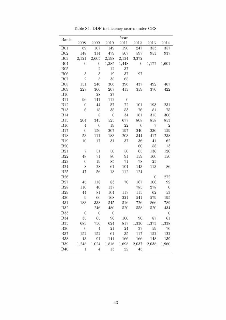
Table S4: DDF ine�ciency scores under CRS

Banks Year2008 2009 2010 2011 2012 2013 2014

B01 69 107 149 190 247 353 357B02 148 314 479 507 597 953 937B03 2,121 2,605 2,598 2,134 3,372B04 0 0 1,385 1,448 0 1,177 1,601B05 2 12 37B06 3 3 19 37 97B07 2 3 38 65B08 151 246 306 396 437 492 467B09 227 366 207 413 359 370 422B10 28 27B11 96 141 112 0B12 0 44 57 72 101 193 231B13 6 15 35 53 76 81 75B14 8 0 34 161 315 306B15 204 345 525 677 808 858 853B16 4 0 19 22 0 7 2B17 0 156 207 197 240 236 159B18 53 111 183 203 344 417 238B19 10 17 31 37 36 41 62B20 60 58 13B21 7 51 50 50 65 136 120B22 48 71 80 91 159 160 150B23 0 19 85 71 78 25B24 8 28 61 104 143 113 86B25 47 56 13 112 124B26 0 272B27 45 118 83 70 167 106 92B28 110 40 137 785 278 0B29 44 81 104 117 115 62 53B30 9 66 168 221 541 579 195B31 183 338 545 516 726 866 789B32 246 480 520 558 520 434B33 0 0 0 0B34 35 65 96 100 90 87 61B35 683 756 624 817 1,336 1,373 1,338B36 0 4 21 24 37 59 76B37 152 152 61 35 117 152 122B38 43 91 144 166 166 148 139B39 1,248 1,024 1,816 1,698 2,037 2,038 1,960B40 1 4 13 22 45

43

Table S5: DDF ine�ciency scores under NIRS

Banks Year2008 2009 2010 2011 2012 2013 2014

B01 62 86 102 138 211 313 293B02 0 0 0 0 139 459 479B03 0 0 0 0 0B04 0 0 288 243 0 0 0B05 2 12 37B06 3 3 19 35 97B07 2 3 30 52B08 21 59 62 181 282 353 392B09 142 211 0 0 0 24 142B10 28 16B11 82 120 53 0B12 0 36 40 45 55 120 133B13 6 15 35 53 75 74 64B14 7 0 0 104 219 128B15 158 239 309 432 506 325 101B16 4 0 19 22 0 4 2B17 0 0 82 103 166 166 83B18 34 24 11 0 133 182 0B19 10 17 31 37 36 40 47B20 32 30 0B21 7 38 40 46 64 122 102B22 28 52 55 66 123 115 102B23 0 1 28 42 56 0B24 8 28 47 81 129 107 73B25 34 30 0 80 119B26 0 231B27 14 95 0 0 157 74 50B28 0 0 127 436 131 0B29 42 69 92 115 105 56 48B30 9 47 96 118 406 517 144B31 0 53 90 108 326 438 324B32 158 202 0 0 130 0B33 0 0 0 0B34 30 59 87 74 88 86 35B35 0 274 147 204 419 362 332B36 0 4 21 24 36 59 69B37 40 32 0 0 88 132 0B38 0 43 38 0 40 3 0B39 0 0 13 0 0 0 0B40 1 4 12 22 45

44

Table S6: DDF ine�ciency scores under VRS

Banks Year2008 2009 2010 2011 2012 2013 2014

B01 62 86 102 138 211 313 293B02 0 0 0 0 139 459 479B03 0 0 0 0 0B04 0 0 288 243 0 0 0B05 1 12 34B06 0 3 19 35 95B07 2 3 30 52B08 21 59 62 181 282 353 392B09 142 211 0 0 0 24 142B10 28 16B11 82 120 53 0B12 0 36 40 45 55 120 133B13 2 14 35 53 75 74 64B14 7 0 0 104 219 128B15 158 239 309 432 506 325 101B16 1 0 11 22 0 4 2B17 0 0 82 103 166 166 83B18 34 24 11 0 133 182 0B19 10 17 31 37 36 40 47B20 32 30 0B21 7 38 40 46 64 122 102B22 28 52 55 66 123 115 102B23 0 1 28 42 56 0B24 4 28 47 81 129 107 73B25 34 30 0 80 119B26 0 231B27 14 95 0 0 157 74 50B28 0 0 127 436 131 0B29 42 69 92 115 105 56 48B30 9 47 96 118 406 517 144B31 0 53 90 108 326 438 324B32 158 202 0 0 130 0B33 0 0 0 0B34 30 59 87 74 88 86 35B35 0 274 147 204 419 362 332B36 0 4 21 23 36 59 69B37 40 32 0 0 88 132 0B38 0 43 38 0 40 3 0B39 0 0 13 0 0 0 0B40 0 4 12 22 45

45

Table S7: HTE ine�ciency scores under CRS

Banks Year2008 2009 2010 2011 2012 2013 2014

B01 1.502 1.797 1.808 1.796 2.056 2.248 2.147B02 1.779 1.902 1.613 1.693 1.721 1.892 1.982B03 1.328 1.000 1.255 1.228 1.475B04 1.000 1.000 1.194 1.276 1.000 1.207 1.286B05 1.170 1.667 1.569B06 1.169 1.312 1.389 1.294 1.378B07 1.167 1.233 1.346 1.384B08 1.401 1.421 1.484 1.591 1.705 1.777 1.780B09 1.793 1.777 1.243 1.248 1.395 1.496 1.438B10 1.792 1.540B11 1.416 1.413 1.186 1.000B12 1.000 1.460 1.561 1.502 1.823 1.860 1.899B13 1.188 1.325 1.497 1.560 1.700 1.787 1.814B14 1.199 1.000 1.179 1.770 2.005 1.561B15 2.285 2.040 1.898 2.063 2.103 1.882 1.828B16 1.168 1.000 1.706 1.819 1.000 1.030 1.024B17 1.000 1.099 1.269 1.380 1.595 1.691 1.646B18 1.644 1.680 1.524 1.319 1.662 1.661 1.263B19 1.395 1.347 1.475 1.402 1.643 1.682 1.709B20 1.265 1.504 1.056B21 1.294 1.469 1.299 1.395 1.415 2.006 2.097B22 1.316 1.389 1.432 1.337 1.318 1.503 1.507B23 1.390 1.335 1.549 1.768 1.680 1.244B24 1.182 1.542 1.484 1.542 1.572 1.497 1.584B25 1.666 1.196 1.029 1.234 1.244B26 1.000 1.916B27 1.278 1.802 1.235 1.247 1.932 1.555 1.635B28 1.274 1.079 1.235 1.617 1.277 1.000B29 1.248 1.474 1.588 1.499 1.710 1.639 1.590B30 1.363 1.763 1.640 1.622 2.024 1.716 1.190B31 1.705 1.662 1.585 1.619 1.334 1.877 1.000B32 2.648 1.963 1.613 1.653 1.809 1.781B33 1.000 1.000 1.000 1.000B34 1.420 1.366 1.403 1.019 1.453 1.551 1.356B35 1.587 1.548 1.431 1.430 1.530 1.541 1.524B36 1.000 1.036 1.300 1.094 1.546 1.892 1.730B37 1.572 1.545 1.251 1.120 1.335 1.455 1.268B38 1.411 1.576 1.414 1.169 1.509 1.684 1.512B39 1.484 1.368 1.000 1.245 1.338 1.002 1.419B40 1.030 1.512 1.632 1.793 2.183

46

Table S8: HTE ine�ciency scores under NIRS

Banks Year2008 2009 2010 2011 2012 2013 2014

B01 1.352 1.405 1.319 1.365 1.594 1.789 1.583B02 1.000 1.000 1.000 1.000 1.109 1.255 1.266B03 1.000 1.000 1.000 1.000 1.000B04 1.000 1.000 1.065 1.033 1.000 1.000 1.000B05 1.170 1.640 1.531B06 1.169 1.233 1.337 1.268 1.376B07 1.167 1.233 1.227 1.256B08 1.030 1.045 1.038 1.048 1.160 1.319 1.416B09 1.277 1.264 1.000 1.000 1.000 1.019 1.091B10 1.562 1.156B11 1.261 1.259 1.073 1.000B12 1.000 1.272 1.207 1.193 1.244 1.272 1.259B13 1.188 1.325 1.402 1.426 1.488 1.494 1.437B14 1.164 1.000 1.000 1.327 1.410 1.165B15 1.497 1.396 1.321 1.400 1.399 1.149 1.034B16 1.168 1.000 1.706 1.809 1.000 1.019 1.024B17 1.000 1.000 1.100 1.170 1.249 1.275 1.196B18 1.213 1.073 1.022 1.000 1.060 1.104 1.000B19 1.324 1.308 1.444 1.386 1.538 1.420 1.324B20 1.083 1.098 1.000B21 1.178 1.230 1.161 1.248 1.300 1.616 1.567B22 1.162 1.215 1.214 1.175 1.225 1.316 1.282B23 1.000 1.004 1.108 1.171 1.181 1.000B24 1.182 1.524 1.278 1.374 1.414 1.385 1.368B25 1.289 1.069 1.000 1.096 1.213B26 1.000 1.371B27 1.059 1.449 1.000 1.000 1.468 1.235 1.144B28 1.000 1.000 1.147 1.000 1.079 1.000B29 1.232 1.323 1.357 1.365 1.461 1.419 1.393B30 1.178 1.278 1.232 1.222 1.490 1.357 1.080B31 1.000 1.049 1.058 1.073 1.198 1.253 1.000B32 1.370 1.226 1.000 1.000 1.046 1.000B33 1.000 1.000 1.000 1.000B34 1.270 1.275 1.204 1.014 1.359 1.413 1.128B35 1.000 1.087 1.049 1.072 1.126 1.057 1.081B36 1.000 1.033 1.300 1.094 1.485 1.592 1.468B37 1.086 1.061 1.000 1.000 1.100 1.170 1.000B38 1.000 1.164 1.070 1.000 1.068 1.004 1.000B39 1.000 1.000 1.000 1.000 1.000 1.000 1.000B40 1.030 1.512 1.632 1.497 1.781

47

Table S9: HTE ine�ciency scores under VRS

Banks Year2008 2009 2010 2011 2012 2013 2014

B01 1.352 1.405 1.319 1.365 1.594 1.789 1.583B02 1.000 1.000 1.000 1.000 1.109 1.255 1.266B03 1.000 1.000 1.000 1.000 1.000B04 1.000 1.000 1.065 1.033 1.000 1.000 1.000B05 1.154 1.640 1.531B06 1.010 1.209 1.337 1.268 1.376B07 1.060 1.209 1.227 1.256B08 1.030 1.045 1.038 1.048 1.160 1.319 1.416B09 1.277 1.264 1.000 1.000 1.000 1.019 1.091B10 1.562 1.156B11 1.261 1.259 1.073 1.000B12 1.000 1.272 1.207 1.193 1.244 1.272 1.259B13 1.091 1.303 1.402 1.426 1.488 1.494 1.437B14 1.164 1.000 1.000 1.327 1.410 1.165B15 1.497 1.396 1.321 1.400 1.399 1.149 1.034B16 1.000 1.000 1.624 1.809 1.000 1.019 1.017B17 1.000 1.000 1.100 1.170 1.249 1.275 1.196B18 1.213 1.073 1.022 1.000 1.060 1.104 1.000B19 1.324 1.308 1.444 1.386 1.538 1.420 1.324B20 1.083 1.098 1.000B21 1.178 1.230 1.161 1.248 1.300 1.616 1.567B22 1.162 1.215 1.214 1.175 1.225 1.316 1.282B23 1.000 1.004 1.108 1.171 1.181 1.000B24 1.099 1.524 1.278 1.374 1.414 1.385 1.368B25 1.289 1.069 1.000 1.096 1.213B26 1.000 1.371B27 1.059 1.449 1.000 1.000 1.468 1.235 1.144B28 1.000 1.000 1.147 1.000 1.079 1.000B29 1.232 1.323 1.357 1.365 1.461 1.419 1.393B30 1.178 1.278 1.232 1.222 1.490 1.357 1.080B31 1.000 1.049 1.058 1.073 1.198 1.253 1.000B32 1.370 1.226 1.000 1.000 1.046 1.000B33 1.000 1.000 1.000 1.000B34 1.270 1.275 1.204 1.014 1.359 1.413 1.128B35 1.000 1.087 1.049 1.072 1.126 1.057 1.081B36 1.000 1.033 1.247 1.070 1.485 1.592 1.468B37 1.086 1.061 1.000 1.000 1.100 1.170 1.000B38 1.000 1.164 1.070 1.000 1.068 1.004 1.000B39 1.000 1.000 1.000 1.000 1.000 1.000 1.000B40 1.000 1.400 1.632 1.497 1.781

48

Table S10: TE ine�ciency scores under CRS

Banks Year2008 2009 2010 2011 2012 2013 2014

B01 1.477 1.814 1.945 1.774 1.994 2.126 2.047B02 2.326 1.873 1.584 1.678 1.700 1.865 1.900B03 1.312 1.325 1.237 1.171 1.289B04 1.000 1.000 1.264 1.249 1.000 1.189 1.265B05 1.368 1.815 1.540B06 1.207 1.393 1.513 1.297 1.327B07 1.203 1.393 1.392 1.362B08 1.510 1.457 1.475 1.484 1.589 1.839 1.873B09 1.852 1.775 1.266 1.232 1.392 1.569 1.475B10 1.801 1.643B11 1.353 1.354 1.152 1.000B12 1.000 1.602 1.544 1.481 1.790 1.831 1.873B13 1.253 1.361 1.652 1.572 1.714 1.811 1.958B14 1.269 1.000 1.247 1.760 1.895 1.538B15 2.282 1.949 1.859 1.985 2.021 1.761 1.693B16 1.198 1.000 1.751 1.946 1.000 1.033 1.032B17 1.000 1.090 1.253 1.357 1.542 1.632 1.679B18 1.803 1.673 1.495 1.310 1.613 1.561 1.248B19 1.495 1.457 1.466 1.381 1.665 1.696 1.836B20 1.256 1.483 1.053B21 1.562 1.459 1.289 1.381 1.398 1.980 2.197B22 1.449 1.419 1.425 1.303 1.275 1.457 1.469B23 1.000 1.336 1.553 1.736 1.526 1.149B24 1.207 1.634 1.472 1.524 1.492 1.472 1.566B25 1.886 1.214 1.032 1.260 1.286B26 1.000 1.827B27 1.288 1.724 1.189 1.201 1.815 1.434 1.497B28 1.289 1.089 1.274 1.497 1.305 1.000B29 1.273 1.517 1.543 1.380 1.563 1.883 1.702B30 1.585 1.838 1.609 1.592 1.932 1.808 1.218B31 1.907 1.921 1.614 1.645 1.779 1.995 2.052B32 2.881 1.901 1.562 1.596 1.737 1.704B33 1.000 1.000 1.000 1.000B34 1.463 1.397 1.349 1.014 1.388 1.612 1.342B35 1.519 1.471 1.372 1.389 1.479 1.488 1.489B36 1.000 1.032 1.288 1.088 1.524 1.908 1.704B37 1.559 1.532 1.245 1.116 1.313 1.385 1.189B38 1.515 1.792 1.390 1.155 1.477 1.683 1.486B39 1.430 1.343 1.402 1.295 1.327 1.485 1.452B40 1.032 1.649 1.706 2.044 2.320

49

Table S11: TE ine�ciency scores under NIRS

Banks Year2008 2009 2010 2011 2012 2013 2014

B01 1.432 1.575 1.474 1.481 1.704 1.838 1.604B02 1.000 1.000 1.000 1.000 1.137 1.334 1.338B03 1.000 1.000 1.000 1.000 1.000B04 1.000 1.000 1.073 1.031 1.000 1.000 1.000B05 1.368 1.778 1.534B06 1.207 1.377 1.467 1.293 1.327B07 1.203 1.377 1.303 1.281B08 1.040 1.053 1.037 1.048 1.158 1.387 1.540B09 1.376 1.339 1.000 1.000 1.000 1.030 1.118B10 1.695 1.222B11 1.263 1.267 1.075 1.000B12 1.000 1.384 1.285 1.258 1.342 1.332 1.329B13 1.253 1.361 1.567 1.506 1.591 1.630 1.636B14 1.252 1.000 1.000 1.345 1.415 1.176B15 1.724 1.444 1.383 1.474 1.377 1.136 1.029B16 1.198 1.000 1.751 1.946 1.000 1.022 1.032B17 1.000 1.000 1.126 1.222 1.239 1.269 1.277B18 1.292 1.105 1.028 1.000 1.055 1.095 1.000B19 1.424 1.423 1.466 1.381 1.614 1.524 1.455B20 1.093 1.140 1.000B21 1.249 1.275 1.176 1.265 1.307 1.721 1.809B22 1.228 1.245 1.214 1.169 1.210 1.316 1.300B23 1.000 1.006 1.132 1.238 1.177 1.000B24 1.207 1.634 1.339 1.409 1.393 1.394 1.409B25 1.408 1.083 1.000 1.113 1.258B26 1.000 1.393B27 1.069 1.520 1.000 1.000 1.457 1.205 1.139B28 1.000 1.000 1.168 1.090 1.096 1.000B29 1.261 1.374 1.362 1.338 1.448 1.605 1.545B30 1.252 1.400 1.347 1.334 1.573 1.444 1.102B31 1.000 1.079 1.096 1.110 1.236 1.366 1.305B32 1.645 1.267 1.000 1.000 1.043 1.000B33 1.000 1.000 1.000 1.000B34 1.366 1.328 1.200 1.011 1.353 1.495 1.138B35 1.000 1.104 1.066 1.092 1.145 1.048 1.079B36 1.000 1.030 1.288 1.088 1.519 1.769 1.586B37 1.121 1.084 1.000 1.000 1.101 1.166 1.000B38 1.000 1.237 1.081 1.000 1.080 1.007 1.000B39 1.000 1.000 1.002 1.000 1.000 1.000 1.000B40 1.032 1.649 1.706 1.688 2.036

50

Table S12: TE ine�ciency scores under VRS

Banks Year2008 2009 2010 2011 2012 2013 2014

B01 1.432 1.575 1.474 1.481 1.704 1.838 1.604B02 1.000 1.000 1.000 1.000 1.137 1.334 1.338B03 1.000 1.000 1.000 1.000 1.000B04 1.000 1.000 1.073 1.031 1.000 1.000 1.000B05 1.088 1.778 1.534B06 1.000 1.377 1.467 1.293 1.324B07 1.125 1.377 1.303 1.281B08 1.040 1.053 1.037 1.048 1.158 1.387 1.540B09 1.376 1.339 1.000 1.000 1.000 1.030 1.118B10 1.695 1.222B11 1.263 1.267 1.075 1.000B12 1.000 1.384 1.285 1.258 1.342 1.332 1.329B13 1.120 1.348 1.567 1.506 1.591 1.630 1.636B14 1.252 1.000 1.000 1.345 1.415 1.176B15 1.724 1.444 1.383 1.474 1.377 1.136 1.029B16 1.000 1.000 1.660 1.941 1.000 1.022 1.022B17 1.000 1.000 1.126 1.222 1.239 1.269 1.277B18 1.292 1.105 1.028 1.000 1.055 1.095 1.000B19 1.424 1.423 1.463 1.381 1.614 1.524 1.455B20 1.093 1.140 1.000B21 1.249 1.275 1.176 1.265 1.307 1.721 1.809B22 1.228 1.245 1.214 1.169 1.210 1.316 1.300B23 1.000 1.006 1.132 1.238 1.177 1.000B24 1.117 1.634 1.339 1.409 1.393 1.394 1.409B25 1.408 1.083 1.000 1.113 1.258B26 1.000 1.393B27 1.069 1.520 1.000 1.000 1.457 1.205 1.139B28 1.000 1.000 1.168 1.090 1.096 1.000B29 1.261 1.374 1.362 1.338 1.448 1.605 1.545B30 1.252 1.400 1.347 1.334 1.573 1.444 1.102B31 1.000 1.079 1.096 1.110 1.236 1.366 1.305B32 1.645 1.267 1.000 1.000 1.043 1.000B33 1.000 1.000 1.000 1.000B34 1.366 1.328 1.200 1.011 1.353 1.495 1.138B35 1.000 1.104 1.066 1.092 1.145 1.048 1.079B36 1.000 1.030 1.225 1.064 1.519 1.769 1.586B37 1.121 1.084 1.000 1.000 1.101 1.166 1.000B38 1.000 1.237 1.081 1.000 1.080 1.007 1.000B39 1.000 1.000 1.002 1.000 1.000 1.000 1.000B40 1.000 1.569 1.688 1.688 2.036

51