centre for economic history the …! 1 trading patterns at the tokyo stock exchange, 1931-1940...

CENTRE FOR ECONOMIC HISTORY THE AUSTRALIAN NATIONAL UNIVERSITY DISCUSSION PAPER SERIES !

THE AUSTRALIAN NATIONAL UNIVERSITY ACTON ACT 0200 AUSTRALIA T 61 2 6125 3590 F 61 2 6125 5124 E [email protected] http://rse.anu.edu.au/CEH

TRADING PATTERNS AT THE TOKYO STOCK EXCHANGE, 1931-1940

JEAN-PASCAL BASSINO ECOLE NORMALE SUPERIERE DE LYON

THOMAS LAGOARDE-SEGOT AIX-MARSEILLE UNIVERSITY

DISCUSSION PAPER NO. 2013-02

FEBRUARY 2013

! 1

Trading patterns at the Tokyo Stock Exchange, 1931-1940

Jean-Pascal Bassino

Institute of East Asian Studies (IAO), Ecole Normale Supérieure de Lyon, 15 parvis René

Descartes, BP 7000, 69342 Lyon, France.

Email: [email protected].

Phone +33 (0) 437 376 039. Fax +33 (0) 437 376 476

and

Thomas Lagoarde-Segot (corresponding author)

Kedge Business School and Aix-Marseille School of Economics, Aix-Marseille University. BP921,

13288 Marseille cedex 9, France.

E-mail: [email protected].

Phone: +33 (0) 491 827 390. Fax: +33(0) 491 827 983

Abstract

This paper relies on daily price indices for stocks and bonds to analyze the functioning of the Tokyo

Stock Exchange (TSE) in the period 1931-1940. Although the TSE was a large and liquid market,

its pricing mechanisms significantly deviated from weak-form efficiency. In this context, zaibatsu

insiders were able to make abnormal returns via informed trading, while other uninformed investors

could rely on technical rules to make abnormal profits. The TSE was a risky financial environment

in which investors adjusted their portfolios significantly in the aftermath of major events. Potential

herding behaviours, price manipulation and reciprocal positive causality (contagion) were observed

across markets. These deficiencies may partially explain Japan’s shift to bank-centered finance after

WWII.

Keywords: emerging stock markets, technical trading, herding, event analysis. JEL code: G14, N25,

! 2


Highlights:

• We analyze the informational efficiency of Tokyo Stock Exchange (TSE) using daily

indices

• Pricing mechanisms significantly deviated from weak-form efficiency

• Using technical trading yielded abnormal profits

• TSE was a risky casino-like financial environment characterized by herding

• These deficiencies may partially explain Japan’s shift to bank-centered finance after WWII

! 3


1. Introduction

Although Japan was still a lower income industrializing country in the 1930s, by the

international standards of the interwar, the Tokyo Stock Exchange (TSE) had become a large and

active market. However, it remains unclear to what extent it was an efficient one. In this paper, we

examine the microstructures of the Japanese financial market from 1931 to1940. This period

corresponds to steady industrialization, rapid increase of military expenditures, an increasing role of

the Japanese army in setting the political agenda, in particular the invasion of Manchuria in 1931,

and the decision to launch a full scale war against China in 1937. The motivation for our

investigation of the functioning of capital markets in pre-WWII Japan is to contribute to the debate

on the respective roles of banks and capital markets in pre-WWII Japan, and on the cause for the

shift to a bank-based financial structure after 1945 (Hamao et al. 2005, Ishii 2007, Okazaki 2007,

Teranishi 2007). In addition, the information generated could contribute to a better understanding of

current financial and political dynamics in the developing world.

We use daily price indices for the three available market segments: ‘industrials’, ‘utilities’, and

‘bonds’. This high frequency dataset was compiled from Japanese yearbooks from the Toyo Keizai

(‘The Oriental Economist’) published in the 1930s and early 1940s. Our results suggest that while

the Tokyo Stock Exchange was relatively large and liquid compared to other markets at that time,

its pricing mechanisms significantly deviated from weak-form efficiency, in a context of persistent

volatility, sudden increases in uncertainty surrounding major economic events, and significant

cross-market spillovers. This overall context of low efficiency made it possible for zaibatsu insiders

to make consistently abnormal returns via informed trading, while other investors could gain from

! 4

adopting technical trading rules. The apparent lack of informational efficiency may be one factor

explaining Japan’s shift to bank-based finance post WWII. Our results also suggest that appropriate

institutional development is a prerequisite for stock markets to efficiently contribute to the

allocation of savings in emerging economies.

Over recent years, an increasing body of empirical research has focused on the historical

exploration of past capital market dynamics in an event analysis approach; for instance, Frey and

Kucher (2000) studied domestic and foreign Austrian, Belgian, French, German, and Swiss bonds

in Zurich Stock Exchange. In a more focused study, Oosterlinck (2003) analyzed the impact of

military developments and political events on French bond market dynamics between 1942 and

1944, using a daily database. His results suggested that the investors’ perception of Vichy France

was primarily affected by De Gaulle’s struggle to gain legitimacy within the Allied forces, rather

than by military developments.1 More recently, some attempts have been made to analyze the

informational dynamics of capital markets prior to the 1950s. Waldenström (2010) looked at the

Danish and Swedish bond markets between 1938 and 1948 and discovered that WWII-related

default costs explained a significant part of sovereign yield spread across markets. Using data

covering the period 1902-1925, Moore (2010) highlighted that firm liquidity levels rather than risk

exposure were an important determinant of cross-section returns in the Madrid and Zurich Stock

Exchanges.

However, all of these authors focused on Western ‘developed’ markets of the time. To the best

of our knowledge, the analysis of informational dynamics and cross-market linkages in TSE we

present in this paper is the first retrospective empirical investigation of a non-Western capital

!!!!!!!!!!!!!!!!!!!!!!!!!!!!!!!!!!!!!!!!!!!!!!!!!!!!!!!!!!!!!1 Other studies have investigated the influence of events on bonds, for instance Brown and Burdekin (2000) on US

bonds during the civil war, Brown and Burdekin (2002) on German bonds traded in London during WWII,

Walderström and Frey (2008) on Nordic (Denmark, Finland, Norway, and Sweden) bonds during the same period.

! 5

market in the pre-WWII period.2 It should be noted that 1930s Japan had shared certain

characteristics with present-day emerging nations: its economy was characterized by low living

standards, uneven wealth distribution, fast capital accumulation, international trade integration, high

political risk, and low transparency.

The remainder of this paper is organized as follows. Section 2 briefly presents the Tokyo Stock

Exchange and the major dynamics affecting the Japanese economy in the 1930s. Section 3 presents

the dataset and employs a battery of econometric tests to analyze informational efficiency levels.

Section 4 analyzes market uncertainty with a focus on sudden endogenous volatility shifts in return

series. Section 5 investigates short-run spillovers among the three segments of the Tokyo Stock

Exchange. Finally, section 6 brings together our conclusions.

2. The TSE in interwar Japan: an emerging market in a newly industrialized country

By the international standard of the interwar, the TSE was a large and active market. The

market value of stocks listed in all Japanese stock exchanges (of which TSE was by far the largest)

was large relative to the GDP, around 1 or above in the 1930s, and the value traded was twice the

GDP. These two indicators were actually higher in Japan than in the US, and a similar pattern can

be observed regarding market turnover (ratio of value traded relative to the market value of stocks

listed). Such market depth and liquidity is astonishing considering the large income gap that existed

between the two countries (Hamao et al. 2005). !!!!!!!!!!!!!!!!!!!!!!!!!!!!!!!!!!!!!!!!!!!!!!!!!!!!!!!!!!!!!2 Ho and Li (2010) looked at breaks in the series of monthly prices for 11 Chinese bonds during the interwar period but

they did not analyze informational efficiency. If could be noted however that their results suggest that military events

related to the successive episodes of the Sino-Japanese conflict had a stronger long term effect than events related to the

civil war, although short term effects were similar. In a related field, Grossman and Imai (2009) performed an event

analysis for turning points in the value of the yen in the 1920s.

! 6

TSE was, however, an emerging market in the interwar.3 Japan already had a long history of

sophisticated financial techniques4, but the development of market capitalization was initially

limited by the reluctance of the most prominent family businesses, the zaibatsu firms, to adopt the

Western style joint-stock company organization and to have a significant part of the shares traded

publicly.5 Non-zaibatsu firms gradually entered the market in the late 19th century by issuing

equities in different fields of activities, in particular banks, railroads, and spinning companies.

However, borrowing remained the dominant source of capital for the non-finance sector until

WWII. The rise in market capitalization became possible around the turn of the century with the

introduction of institutional innovations. The establishment of securities companies6 created

conditions which facilitated the issuance of equities and short-term investment. The rise in market

capitalization was also spurred by the adoption of the new commercial code of 1899 stipulating that

equities should be marketable (Miyamoto 1984, 56), and by the opening the financial market to

foreign investors.7

The expansion of Japan’s manufacturing activities and international trade accelerated during

WWI as a result of the drastic decline of European export to Asia that which was a consequence of

!!!!!!!!!!!!!!!!!!!!!!!!!!!!!!!!!!!!!!!!!!!!!!!!!!!!!!!!!!!!!"!TSE was initially established, in 1878, at the initiative of Shibuzawa Eichi, a prominent non-zaibatsu entrepreneur of

the Meiji era, as a joint stock company dealing mainly with public bonds issued for compensating the samurai for the

loss of their stipends as a result of early Meiji institutional changes (Masaki 1973, 10).!

4 Formally organized rice futures markets existed in Osaka from the mid 18th century (Hamori et al. 2001).

#!Zaibatsu firms dominated certain sectors, in particular mining, shipbuilding, shipping, and international trading, and

were also extremely active in banking and insurance companies, collecting a sizable share of private savings, and

making capital available to companies of the same group (Mitsubishi, Mitsui, Sumitomo, Yasuda…). On zaibastu

finance, see for instance Asajima (1984) and Sugiyama (1985), !

$!The first one, in 1897, was Koike Shoten (Koike Securities), the forerunner of Yamaichi securities (Noda 1978, 93).!

%!In 1906, Hokkaido Mining and Kansai Railways issued the first private bonds denominated in British pounds; these

bonds were partly subscribed in by British investors such as the Chartered Bank of Japan, Australia, and China (Noda

1978, 100).!

! 7

the conflict and the rising cost of freight for transoceanic shipping. These new conditions created

opportunities for new ventures financed through the issuance of equities, resulting in a rapid

expansion of market capitalization (Figure 1). The uneven income distribution contributed to high

levels of saving and capital accumulation, in a trend culminating during WWII (Moriguchi and Saez

2008). The development of equity markets continued after WWI. In 1921, for the first time, a

Zaibatsu firm (Mitsubishi Mining) offered common stocks to the general public of subscribers; the

number of shareholders rose dramatically from 28 to 7955. Mitsubishi Gomei (partnership

company) still controlled 60% of paid up capital, but the figure was down from 97.5% in 1920

(Masaki 1978, 43).8 Other zaibatsu groups gradually followed this example during the 1920s and

early 1930s.

This new approach of zaibatsu firms to equity markets set a momentum leading to a steady rise

in market capitalization and the emergence of the TSE, a sizable and active capital market for

equities. The reliance on debt in the private non-financial sector (ratio of borrowing to equities and

investments) declined sharply during the interwar period from an average of 1.58 in the period

1916-20 to 1.18, 1.09, 0.93, and 0.85 in 1921-1925, 1926-1930, 1931-1935, and 1936-1940

respectively. For leading companies, the ratio was actually much lower, ranging from 0.21 to 0.33

(Fujino and Teranishi 2000, appendix).

Figure 1 around here

In the meantime, public investment had also expanded, largely funded through the issuance

of public bonds (Figures 2 and 3). After the suspension of the gold convertibility of the yen, in

!!!!!!!!!!!!!!!!!!!!!!!!!!!!!!!!!!!!!!!!!!!!!!!!!!!!!!!!!!!!!&!The rise in equity capitalization was further amplified by the development a new generation of Zaibatsu (shinko

zaibatsu) that lacked capital, as exemplified in1928 by the public sales of stocks of Nissan’s holding company (Clark

1979, 78).!

! 8

1931, a deliberate policy of budgetary expansion resulted in the massive issuance of public bonds

(Cha 2003), mostly underwritten by the Bank of Japan, but gradually sold on a secondary market

(Tomita 2005). This trend was amplified by the militarization of the economy9 that resulted in a

sustained demand for manufactured goods (aircrafts, explosives, machinery, motor vehicles,

shipbuilding). However, it was not until late 1930s that total market capitalization of public bonds

became larger than stock market capitalization.

In the context of the militarization of the economy and political instability10 of the 1930s,

the concentration of financial power in the hands of a few individuals, the main shareholders of the

zaibatsu business groups (plus a number of non-family managers of these firms), resulted in low

transparency for the TSE.11 As Teranishi (2007, 50) points out “while stock markets played a role in

corporate governance, … resource allocation functions were only exhibited within a narrow group

of wealthy individuals.” But, in the meantime, the activity of the major banks controlled by

industrial business groups (described as “organ bank” or “main bank” by economic historians)

consisted largely in “connected lending” (ibid 61). Kinship-based social networks were therefore

determinant in financial resource allocation. The interlocking of shareholders and managers

between banks and non-banking companies, which resulted in poor bank performances, has been

regarded as a major cause of the financial crisis of 1927 (Okazaki et al. 2005).12 The development

!!!!!!!!!!!!!!!!!!!!!!!!!!!!!!!!!!!!!!!!!!!!!!!!!!!!!!!!!!!!!'!The rapid rise of military expenditures, both in absolute terms and as a percentage of total public expenditures, was

largely the consequence of a decision made within the military circle, without government approval, to invade

Manchuria in 1931 and to launch a full-scale war against China in 1937. !

10 In particular, the assassination of political figures and top bureaucrats by young activist army and marine officers, and

an attempted military coup d’état in February 1936.

((! During the 1930s, zaibatsu groups increased their centralized control of the economy through connections with

military oligarchy. Cartels were legally encouraged under the Major Industries Control Law and the Industrial

Association Law of 1931.!

12 The Showa financial crisis resulted in the bankruptcy of thirty-seven banks, and the collapse of the Suzuki zaibatsu.

! 9

of equity markets in the 1930s can therefore be regarded as a response on behalf of non-financial

firms to the inability of the banking sector to serve efficiently the needs of industrial firms engaged

in massive programs of investment. However, little is known about TSE trading patterns. The rest

of this paper therefore explores the market’s microstructures by means of a battery of empirical

tests.

Figures 2 and 3 around here

3. Informational efficiency in the Tokyo Stock Exchange

We rely on a high frequency database for the TSE using daily price composite indices for three

segments of the market: ‘industrials’, ‘utilities’, and ‘bonds’ for the period ranging from 1/1/1931 to

31/12/1940. The dataset was taken from yearbooks in Japanese from the Toyo Keizai (‘Oriental

Economist’) published in the 1930s and early 1940s. The composite indices provided in this source

are reported as calculated using information on 25 to 30 industrial companies, 25 utilities

companies, and 4 to 5 types of central government bonds (4 types in 1931-1934, 5 thereafter (the

name of the companies and the detail of the bonds is not reported). The market was open from

Monday to Saturday (except bank holidays), with a few unexplained closures for industrial shares.

After the careful removal of inconsistent data points, we calculated returns on day t as !! !

!" !!!!!!

where !!is the closing value of the selected index.

!!!!!!!!!!!!!!!!!!!!!!!!!!!!!!!!!!!!!!!!!!!!!!!!!!!!!!!!!!!!!!!!!!!!!!!!!!!!!!!!!!!!!!!!!!!!!!!!!!!!!!!!!!!!!!!!!!!!!!!!!!!!!!!!!!!!!!!!!!!!!!!!!!!!!!!!!!!!!!!!!!!!!!!!!!!!!!!!!!!!!!!!!!!!!!!!!!!!!!!!!!Okazaki and Sawada (2006) argue that “policy-promoted consolidation was likely to be accompanied by large

organizational costs”.

! 10

Table 1 around here

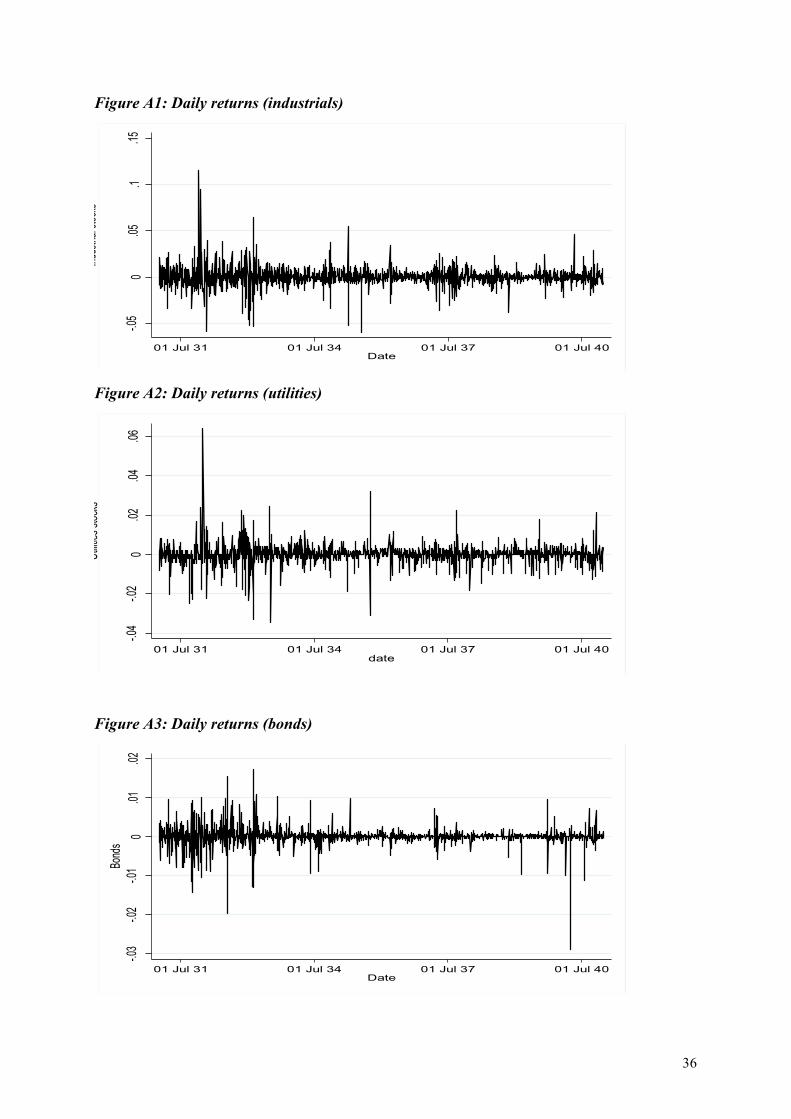
Table 1 displays summary statistics for the obtained returns. The industrial market segment

posted the highest absolute mean returns over the study period. However, the bond market tended to

outperform the two others in terms of risk-adjusted returns as shown by the Sharpe ratio. The level

of volatility, 0.009 and 0.004 and 0.002 for the industrial and utilities indices, respectively, is

similar to those observed in small contemporary emerging markets, for instance Morocco (0.008)

and Tunisia (0.005) in 2004-2009 (Abdmoulah. 2010). Positive skewness in the industrials and

utilities markets suggests that investors tended to overvalue good news and undervalue bad news.

Not surprisingly, we observe lower volatility levels in the bond market (0.002), which is also the

only one displaying negative skewness. This suggests different behavioral patterns of stock and

bond market investors, with higher relative risk-aversion levels for bond investors.

All return series tend to strongly depart from normality, also a commonly observed feature

in emerging markets. We also find significant levels of excess kurtosis in all markets, which implies

that a high level of the observed variance is due to extreme deviations from the mean as opposed to

frequent smaller deviations. Evidence of non-normality echoes current debates on the accuracy of

applying standardized asset pricing and risk analysis techniques, e.g.. CAPM and the Black-Scholes

Option Pricing Model (Ellis and Sundmacher 2011).

We analyze weak-form informational efficiency levels more formally through a set of non-

parametric variance ratio tests for the random walk hypothesis13. In particular, Wright’s (2000) test

based on ranks was shown to have high power against a wide range of models displaying serial

!!!!!!!!!!!!!!!!!!!!!!!!!!!!!!!!!!!!!!!!!!!!!!!!!!!!!!!!!!!!!13 Our analysis focuses on the weak form of efficiency hypothesis, which states that price changes are random and have

no links to past prices. Rejecting the weak form of informational efficiency suggests a rejection of the semi-strong form

(under which price changes reflect all public information) and the strong form (under which price changes reflect both

public and private information) of market efficiency.

! 11

correlation and is robust in the case of non-normal time series. We report test statistics for different

holding periods14.

To further document efficiency levels, we complement this analysis with a simulation

exercise in which a Japanese investor ignores economic fundamentals and follows a purely

technical approach to trading. We assume that the Japanese investor follows a variable moving

average (VMA) rule, in which an investor takes a long position if the short-term VMA is above the

long-term VMA, and exits the market otherwise. This rule is described in equation 1.

!"

!#

$

!%

!&

'(

= ) )= =

**

otherwise

PL

PS

ifI

S

s

L

lltst

t

0

1111 1

(1)

In (1), S and L stand for short and long-term, respectively. Following Brock et al. (1992), we select

1_50, 1_150, 5_150, 1_200 and 2_200 as VMA rules, where 1, 2 and 5 represent the number of

days in the short-term moving average and 50, 150 and 200 the number of days in the long-term

moving average. When a ‘buy’ signal is generated, the investor buys the share and holds it until a

sell signal is generated, at which time he exits the market. We assume that the borrowing and

lending rates are the same and that the risks during buying and selling periods are the same. The

return for this strategy is given by ( ) !!"

#$$%

&'''!!

"

#$$%

&'= +

'+

+ 111 11

11

t

ttt

t

ttt P

PIIPPIµ . Such rules are often

used in empirical testing of market efficiency as they can sometimes pick up some of the hidden

patterns that are not detected by linear models (Chang et al, 2004; Lagoarde-Segot and Lucey,

2008). Following Brock et al (1992), the t-statistic is:

!!!!!!!!!!!!!!!!!!!!!!!!!!!!!!!!!!!!!!!!!!!!!!!!!!!!!!!!!!!!!14 As a robustness check we also ran the Kalman filter test of evolving efficiency from Zalewska-Mitura and Hall

(1999). Results are available upon request.

! 12

s

s

b

b

sb

nn

BS22 !!

µµ

+

"=

(2)

With !+

=+=

1

01

,,

1 n

ttt

sbsb IRn

µ , and ( )!+

=+ "=

1

0

2,1

,

2,

1 n

ttsbt

sbsb IRn

µ# .

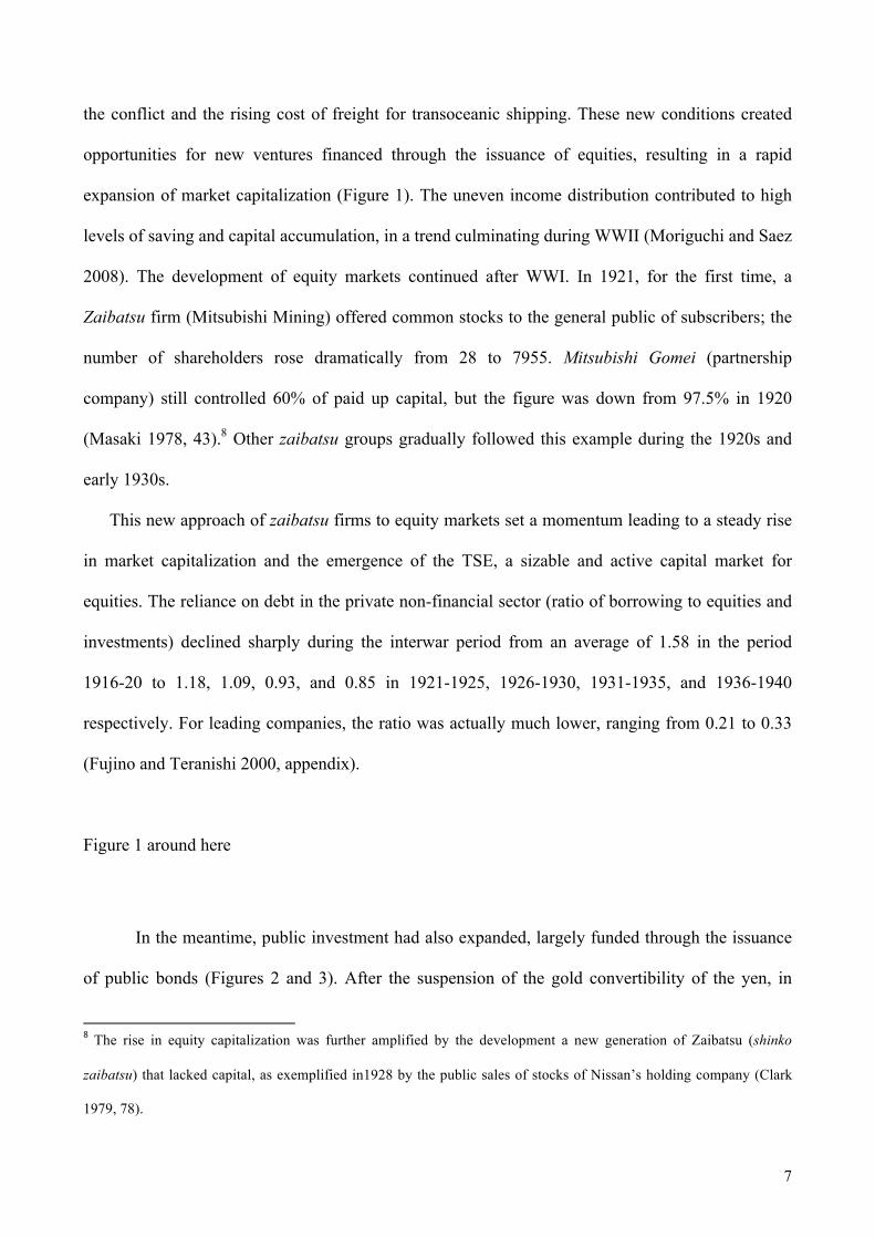
A rule is deemed to be effective if returns following a buy signal are significantly higher than

returns for the sell signal and those obtained via a buy and hold strategy.

Results for the static efficiency tests are shown in table 2 and indicate a clear departure from

informational efficiency. This can be explained by the specific institutional context. Disclosure

requirements were lax as evidenced by the absence of listing criteria other than the number of years

since establishment, total face value, total paid-up value, and number of stocks (Hamao et al. 2005).

Since neither reporting nor auditing was required, we can assume segmentation in access to

information existed between zaibatsu and non-zaibatsu investors. In addition, table 3 reports results

from the technical trading rules. Results show that ex-post returns are significantly higher for buy

signals than for the sell signals, and consistently beat the buy-and-hold strategy. These results

suggest that it would have been rational for uninformed, non-zaibatsu investors (such as wealthy

rural landlords) to adopt trading strategies disconnected from economic fundamentals, given the

context of low informational disclosure and centralized corporate governance. Such strategies may

explain the high level of volatility documented earlier.

Tables 2 and 3 around here

4. Uncertainty and volatility shifts

! 13

In a second strand of analysis, we study the presence of sudden shifts in volatility and relate

them to major economic, corporate and political events using the ICSS algorithm of Inclan and Tiao

(1994) and Bacmann and Dubois (2001). Over recent years, this technique has become common

practice for exploring volatility dynamics in emerging markets. Inclan and Tiao’s (1994) Iterative

Cumulative Sum of Squares (ICSS) algorithm assumes that a time series of interest has a stationary

unconditional variance over an initial time period until a sudden break takes place.15 However, it

has been shown that the ICSS algorithm is biased towards finding too many breakpoints caused by

serially correlated volatility (Bacmann and Dubois 2001). Following standard practice (e.g.

Fernandez, 2007) we first filter the data by fitting an AR(1) model with a GARCH(1,1)

specification for the conditional variance of innovations. We then apply the ICSS algorithm to the

standardized residuals obtained from the estimation. As an additional robustness check, we

incorporated the detected volatility breaks in a model for market returns16:

2121111

1

... !!

!

+++++=

+++=

ttnnt

tttt

ehDdDdhehrr

""#

#$"

(1)

Equation (1) describes the stock return mean tr that depends on an autoregressive process as

well as a risk premium parameter ! capturing the tradeoff between volatility and returns. Returns

volatility is measured by conditional variance ht, which has three components: a constant, an

autoregressive term (the GARCH term), and the last period’s squared residual (the ARCH term). !!!!!!!!!!!!!!!!!!!!!!!!!!!!!!!!!!!!!!!!!!!!!!!!!!!!!!!!!!!!!(#!See appendix 2 for a detailed presentation!

($!As shown in appendix 2, we first specified a simple AR (1) model for each series and implement ARCH-LM test for

serial correlation in the residuals. In each market, we found serial dependence in the mean and in the residuals. This

suggests that a GARCH(1,1) model coupled with an autoregressive process is an appropriate modeling strategy for

Japanese stock returns. The GARCH-in-mean specification is chosen in order to take into account the theoretical

relationship between risk and returns. The latter is captured by the parameter !.

! 14

The sum !! ! !! captures the degree of volatility persistence. !!!!! are the dummy variables: 1

for each point of sudden change of variance onwards and 0 for otherwise.

We estimated GARCH-M (1.1) models for the three markets (Appendix 2, Table A2).

Following Wang and Moore (2008), we report three model specifications: one model without any

volatility shift, one model including all the identified shocks, and a model including only the

significant shocks. Inspection of this table shows that " is significant at the 1% level for the three

markets when dummies are not included. This confirms previous results pointing to a lack of

informational efficiency. In addition, the risk premium parameter ! is consistently insignificant in

all markets except the utilities market, where shocks on the previous period’s variance significantly

impact daily returns. This suggests that Japanese investors included a risk premium parameter in

their utilities portfolio choices, perhaps to compensate for lower informational efficiency levels.

Turning to the variance equation, we find that GARCH-M (1,1) effects (ARCH and

GARCH) are significant for all markets. Measures of volatility persistence given by !! ! !! are

very close to 1 for the standard GARCH-M (1,1) without regime shifts, indicating extreme

persistence in volatility. As expected, volatility persistence is lower when we incorporate the regime

shifts detected by the ICSS algorithms. However, we find that these shocks account for about 25%

of volatility persistence in the Tokyo Stock Exchange; a small figure when compared with results

obtained for contemporaneous emerging markets. For instance, using a similar methodology, Wang

and Moore (2009) found that volatility persistence was reduced up to 67.3% (for Slovakia) in a

panel of five Central European emerging markets.

In addition, GARCH effects remain significant when dummy variables are introduced for

the three markets. This is to be contrasted with the seminal study by Aggarwal et al. (1999), which

detected that these effects were eliminated in eight countries out of a sample of sixteen emerging

markets for the 1985-1995 period. Ljung-Box statistics performed on standardized residuals (Also

in Appendix 2, Table A2) reveals that there is still significant autocorrelation in the residual series.

! 15

This result is common for thinly traded emerging markets: applying a similar GARCH-M(1,1)

filter, Abdmoulah (2010) found significant autocorrelation in the least liquid emerging markets of

the Middle East and North Africa (MENA) region (Tunisia and Jordan). Taken together, these

results suggest significant volatility persistence in the 1930s Tokyo Stock Exchange. This may be

explained by lower liquidity, higher transaction costs, lower efficiency, and greater segmentation, in

an overall context of high uncertainty. By 21st century standards, the 1930s Tokyo Stock Exchange

could thus be considered a ‘frontier market’.

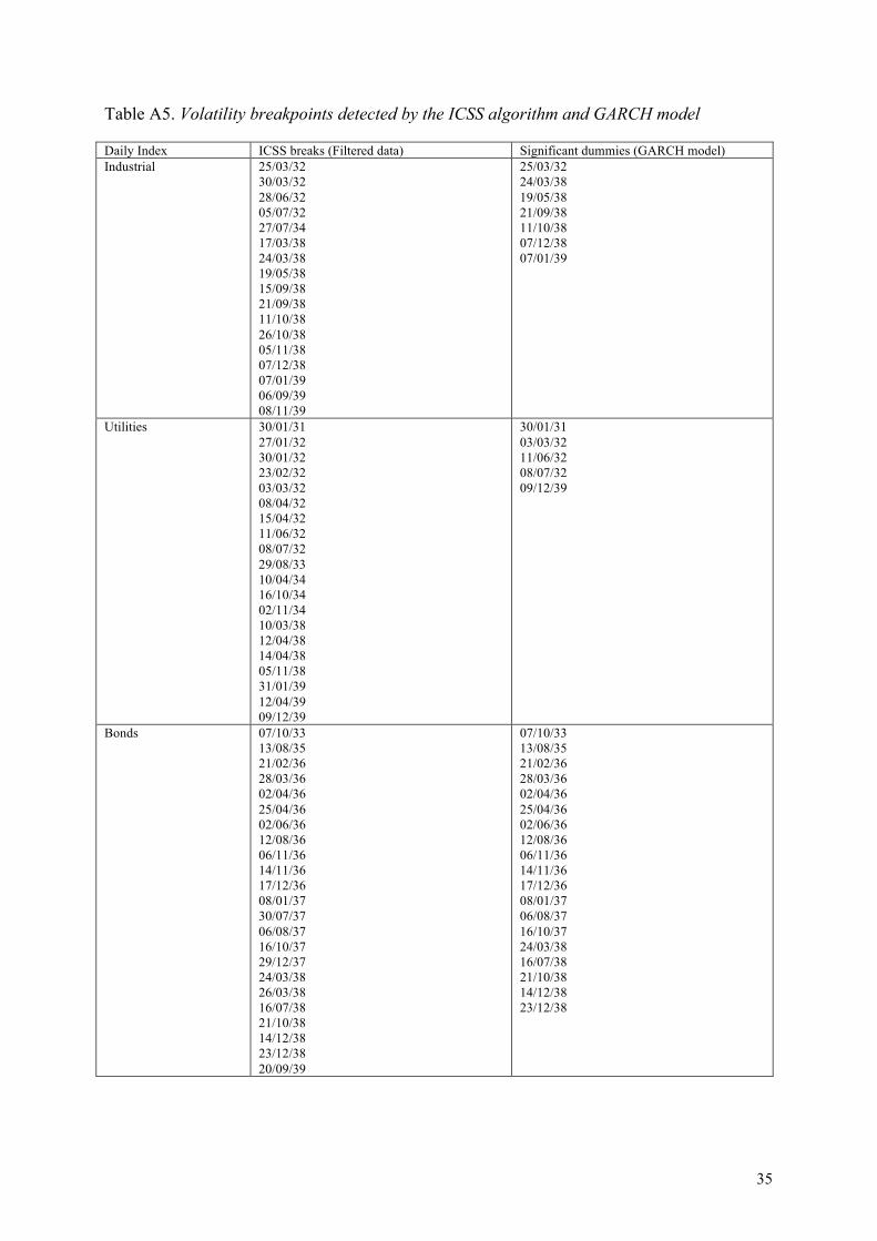
We then consider the robust endogenous volatility shifts hence identified and associate them

to significant economic, financial, and political events (Table 4)17. In order to reduce arbitrariness in

the selection of events, we relied on annual chronologies reported in the Toyo Keizai yearbook and

retained events occurring either the same day or during the previous two or three working days,

excluding therefore Sundays and bank holidays.18 We selected as a presumably related event the

most plausible candidate at the closest date of the break. This means that we omitted information on

date of implementation of decision already announced previously, or events with a scope limited to

a particular sector in the case of bond series.19

Table 4 around here

The main information obtained from this exercise is that the volatility shifts were essentially

influenced by political decisions with strong economic implications. Neither the invasion of

Manchuria (September 19, 1931) nor the outbreak of the Sino-Japanese war (July 7, 1937) are

!!!!!!!!!!!!!!!!!!!!!!!!!!!!!!!!!!!!!!!!!!!!!!!!!!!!!!!!!!!!!17 Results from the ICSS algorithm analysis and GARCH model appear in appendix 2.

(&!For a few cases (e.g. break of 07/10/33 on bonds series), we went further back in time to identify a plausible date.!

('!E.g., decision by cotton textile producers to establish a fund for the development of textile production in Manchuria.!

! 16

identified as having an impact on equities or bonds traded in the TSE. The same remark applies to

the attempted coup d’état of February 26, 1936 which is not associated with a break. These results

echo the findings presented in papers looking at events affecting bonds series in WWII Europe but

with an even stronger relation to economic policy.20

5. Cross-market spillover

This section investigates short run linkages between the three segments of TSE (industrial,

utilities, and bonds). We adopt a VAR modeling approach to model shock transmissions in the

Japanese financial markets via the inspection of generalized impulse response functions and

variance decomposition analysis.21 Stationarity analysis rules out the possibility that the series may

be cointegrated given that logged prices are found to be stationary with a drift. In the absence of ex-

ante information on the causal structure of shock transmission in the three financial markets, we set

the variables of interest at the top of the Xt vector to derive General Impulse Response Functions

(GIRF). However, the forecast error variance decompositions of a GIRF do not sum up to unity.

Therefore we adopted the practice of Hasbrouck (1995) for variance decompositions by

sequentially ordering each market first in the system to obtain the maximum share of its innovation

and then order it last in the system to obtain its minimum share. The average of the maximum and

minimum shares becomes the final single decomposition share of the innovation.

Examination of the Granger causality results (Table 5) suggests the existence of significant

linkages across markets. We find bidirectional causality between the bond and industrial markets as

!!!!!!!!!!!!!!!!!!!!!!!!!!!!!!!!!!!!!!!!!!!!!!!!!!!!!!!!!!!!!)*!Purely political events had little influence on the series. The sole exception is the formation of the Hiranuma cabinet

in January 1939. For a general presentation of the political context and main events of the 1930s, see for instance Sims

(2001).!

21 For robustness, we also used a DCC GARCH model. Methodology and results are presented in Appendix 4.

! 17

well as between the industrial and utilities markets. We also find unidirectional causality running

from the bond to the utilities markets. This indicates that although equity capitalization was larger

than that of bond market, the latter was dominant.

Table 5 and Figure 4 around here

Inspection of Generalized Impulse Response Functions shows that contemporaneous shocks

occurring in the utilities and industrials markets have a significant impact on the bond market

(Figure 4). Shocks to the bond and utilities markets have a significant impact on the industrial

market, while shocks to the bond and industrials markets have a significant impact on the utilities

markets. All shocks are positive, suggesting herding behavior and a lack of portfolio diversification

opportunities. However, these volatility spillovers die out two to four trading days after the initial

shock.

Turning to the Variance Decomposition Analysis, we find that the industrial and utilities

market are less endogenous than the bond market (Table 6). Shocks to their own past values explain

up to 89% of forecast error variance as opposed to 96% in the bond market. Utilities market

dynamics explain up to 15% of the industrial market, while the industrial market explains up to

13% of the utilities market, suggesting higher integration in the two stock market indices. By

contrast, our results reveal a sharp segmentation between stock and bond markets. The industrial

and utilities indices only explain up to 2.28% and 2.26% of the bond market’s variance,

respectively.

The lack of transparency appears as the most likely explanation for both herding behavior

and market segmentation. Two types of investors were operating in the TSE. On the one hand,

controlling families of zaibatsu firms that had access to insider information, a critical asset in an

institutional context characterized by the insufficient reporting by listed companies and absence of

! 18

external auditing. These investors had access to information on the performances of industrial and

utilities companies, but they also had strong incentives to maintain family shareholding at a stable

level, at least for the core companies of the zaibatsu group.

On the other hand, the mass of minor investors, in particular rural landlords and other

wealthy mid-size players that had no access to insider information on equities. Unfortunately, their

behavior is not documented by strong evidence. Our conjecture is that these investors had little

choice but to adopt a casino-like approach, selecting assets on the basis of the most dependable

information available to them, bonds related events, taking bets on spillover effects from bonds to

equities.

6. Conclusion

The objective of this paper was to shed light on the functioning pre-WWII Japanese capital markets

by conducting an empirical investigation of market microstructure. We first analyzed informational

dynamics using variance ratio tests and technical trading analysis and significantly rejected the

weak-form efficiency hypothesis. We then used the ICSS algorithm of Inclan and Tiao (1994) and

Bacmann and Dubois (2001) and then detected a number of regime shifts in volatility surrounding

major economic, corporate, and political events. Results from a GARCH-M (1,1) model confirmed

the presence of relatively low informational efficiency levels and significant volatility persistence,

especially surrounding major economic events. Overall, these results suggest the presence of

permanent behavioral biases in the Tokyo Stock Exchange. Finally, we modeled cross-market

linkages via the inspection of generalized impulse response functions and variance decomposition

analysis derived from a SVAR model. These results indicated significant short-run spillovers across

markets, suggesting that sudden rises in uncertainty created ‘financial contagion’ across the various

! 19

segments of TSE. Overall, this analysis suggests that the TSE was similar to an emerging market, in

the sense that a lack of informational efficiency caused investors to significantly adjust their

portfolios in the aftermath of major events, with potential herding, price manipulation and

reciprocal positive causality (contagion) across markets.

Turning back to the debate on the cause of the shift to bank-centered finance after 1945, two

complementary interpretations could be considered in the light of our findings. Since both banks

and capital markets were apparently quite inefficient in interwar Japan, the shift could be due to a

change in relative (in)efficiency. A first possible explanation of the dominant role of banks in

postwar Japan is that the policy of “dissolution of the zaibatsu” implemented by the US occupation

authorities in 1945 resulted in effect in a loss of power (and wealth) for the controlling families that

played a key role in the both banks and capital markets in the interwar. The interlocking of

management and shareholding of large firms did not disappear but the kinship-based social

networks that determined the flow of “connected lending” in the interwar became irrelevant.

However, the same remark applies to the flow of insider information on equity markets. A second

explanation for the postwar shift to bank centered finance, which is complementary rather than

contradictory, could be that, under strict supervision by the Ministry of Finance and the Bank of

Japan in the post-WWII period, banks became able to provide financial services in a more efficient

way.

! 20

Acknowledgements

We thank participants at the 2012 Economic History Society Meeting in Oxford (UK), the 2012 INFINITI conference on International Finance at Trinity College Dublin (Ireland) and the 2012 Asian Historical Economics Conference at Hitotsubashi University (Japan) for their useful comments and discussions on earlier versions of this paper.

References

Abdmoulah, W., 2010. Testing the evolving efficiency of 11 Arab stock markets. International Review of Financial Analysis, 19 (1), 25-34.

Aggarwal. R., Inclan. C., Leal. R., 1999. Volatility in emerging stock markets. Journal of Financial and Quantitative Analysis, 34. 33-55.

Asajima S., 1984. Financing of the Japanese zaibatsu: Sumitomo as a case study in Okochi A. and Yasuoka S. (Eds), Family business in the era of industrial growth, Tokyo, University of Tokyo Press, 95-120.

Bacmann. J., Dubois, M., 2002. Volatility in Emerging Stock Markets Revisited. Paper presented at the European Financial Management Association London. http://ssrn.com/abstract=313932!

Brock, W., Lakonishok, J., LeBaron, B., 1992. “Simple technical trading rules and the stochastic properties of stock returns”. Journal of Finance 47, 1731–1764.!

Brown, W.O. and Burdekin, R.C.K., 2000. Turning points in the U.S. civil war: a British perspective. Journal of Economic History, 60(1), 216-231.

Brown, W.O., Burdekin, R.C.K. 2002. German debt traded in London during the Second World War: a British perspective on Hitler. Economica, 69(276), 655-669.

Cha, M-S., 2003. Did Takahashi Korekiyo rescue Japan from the Great Depression? Journal of Economic History, 63(1), 127-144.

Chang, E.J., Lima, E.J.A., Tabak, B.M., 2004. Testing for the predictability of emerging equity market . Emerging Markets Review 5, 295-316.

Clark R., 1979. The Japanese Company. Tokyo, Tuttle. Ellis, C., Sundmacher, M., 2011. “Dependence and return distributions during crises”, in Batten, J.,

A., Szilagyi P. G., (Ed.) The Impact of the Global Financial Crisis on Emerging Financial Markets (Contemporary Studies in Economic and Financial Analysis, Volume 93), Emerald, 449-471.

Fernandez, V., 2007. Stock market turmoil: worldwide effect of Middle-East conflicts. Emerging Markets Finance and Trade. 43(3), 58-102.

Frey, B.S. and Kucher, M., 2000. History as reflected in capital markets: the case of World War II. Journal of Economic History, 60(2), 468-496.

Fujino, S., Teranishi, J., 2000. Nihon kinyu no suryo bunseki (Quantitative analysis of Japanese finance). Tokyo: Toyo Keizai.

Grossman, R.S., Imai, M., 2009. Japan’s return to gold: turning points in the value of the yen during the 1920s. Explorations in Economic History, 46 (3), 314-323.

Hamao, Y., Hoshi, T., Okazaki, T. 2005. The genesis and development of capital market in pre-war Japan. University of Tokyo, Discussion paper CIRJE F-320 (original Japanese version: Okazaki, T., Hamao, Hoshi, T. 2004.

Hamori, S., Hamori, N. Anderson, D.A., 2001. An empirical analysis of the efficiency of the Osaka rice market during Japan's Tokugawa era. Journal of Future Markets 21, 861-874.

Historical Statistics of Japan (online version), Ministry of internal Affairs and Communications; http://www.stat.go.jp/english/data/chouki/index.htm

! 21

Ho, C-Y, Li, D. 2010. Marching in the storm: the Chinese bond market 1918-1942. Paper presented at the Economic History Society annual conference, University of Durham.

Inclan. C., Tiao. G.C. 1994. Use of cumulative sums of squares for retrospective detection of changes of variance, Journal of the American Statistical Association, 89. 913-923.

Ishii, K. 2007. Equity investment and equity investment funding in prewar Japan; comments on Were banks really at the center of the Japanese financial system in prewar Japan? Monetary and Economic Studies, March.

Lagoarde-Segot, T., Lucey, B., 2008. Efficiency in emerging markets: evidence from the MENA region. Journal of International Financial Markets, Institutions and Money 18, 94-105

Masaki H., 1973, Nippon no kabushiki kaisha kinyu (Corporate finance in Japan). Kyoto, Mineruva Shobo.

Masaki H., 1978. The financial characteristics of the zaibatsu in Japan: the old zaibatsu and their closed finance, in Nakagawa K. (Ed.), Marketing and finance in the course of industrialization, Tokyo, University of Tokyo Press, 33-54.

Miyamoto M., 1984, The position and role of family business in the development of Japanese company system, in Okochi A. & Yasuoka S. (Eds), Family Business in the Era of Industrial Growth, Tokyo, University of Tokyo Press, 39-92.

Moore, L., 2006. The effect of World War One on stock market integration. Mimeo. Moriguchi, C., Saez E. 2008. The evolution of income concentration in Japan, 1885-2002: evidence

from income tax statistics. Review of Economics and Statistics, 90, 4, 713-734. Noda M., 1978, Corporate finance of railroad companies in Meiji Japan, in Nakagawa K. (Ed,),

Marketing and finance in the course of industrialization, Tokyo, University of Tokyo Press, 87-101.

Okazaki, T. 2007. The evolution of corporate finance and corporate responsibility on prewar Japan: comments of “Were banks really at the center of the Japanese financial system in prewar Japan?” Monetary and Economic Studies.

Okazaki, T, Sawada, M. 2006. Effects of a bank consolidation promotion policy: evaluating bank law in 1927 Japan. University of Tokyo, Discussion paper CIRJE F 400.

Okazaki, T, Sawada, M., Yokoyama, K. 2005. Measuring the extent and implications of director interlocking in the pre-war Japanese banking industry. Journal of Economic History, 65(4), 1082-1115.

Oosterlinck, K. 2003. The bond market and the legitimacy of Vichy France. Explorations in Economic History, 40 (3), 326-344.

Sims, R. 2001. Japanese political history since the Meiji renovation 1868–2000. Palgrave, Macmillan.

Sugiyama K., 1985. Shipbuilding finance of the shasen shipping firms: 1920’s-1930’s, in Yui T. & Nakagawa K. eds, Business history of shipping, Tokyo, University of Tokyo Press, 255-277.

Teranishi, J. 2007. Were banks really at the center of the Japanese financial system in prewar Japan? Monetary and Economic Studies, March, 49-76

Tomita, T. 2005. Direct underwriting of government bonds by the Bank of Japan in the 1930s. Nomura Research Institute, NRI Paper 94.

Toyo Keizai, 1932. Oriental Economist Economic Yearbook 1932 [東洋経済経済年報昭和7年, Toyo Keizai Keizai Nenpo showa 7nen], 117-118.



! 22








Waldenström, D., 2010. Why does sovereign risk differ for domestic and external debt? Evidence from Scandinavia, 1938–1948. Journal of International Money and Finance. 29 (3), 387-402.

Waldenström, D., Frey, B.S., 2008. Did Nordic countries recognize the gathering storm of World War II? Evidence from the bonds markets. Explorations in Economic History, 45(2), 107-126.

Wang, P., Moore, T., 2009. Sudden changes in volatility: The case of five central European stock markets. Journal of Multinational Financial Management. 19 (1), 33-46.

Yasuoka, S., 1984. Capital ownership in family companies: Japanese firms compared with those in other countries, in Okochi A. & Yasuoka S. (Eds.), Family business in the era of industrial growth, Tokyo, University of Tokyo Press, 1-37.

Zalewska-Mitura, A., Hall, S.G., 1999. Examining the first stages of market performance: a test for evolving market efficiency, Economics Letters, 64- 1, 1-12.

! 23

FIGURES

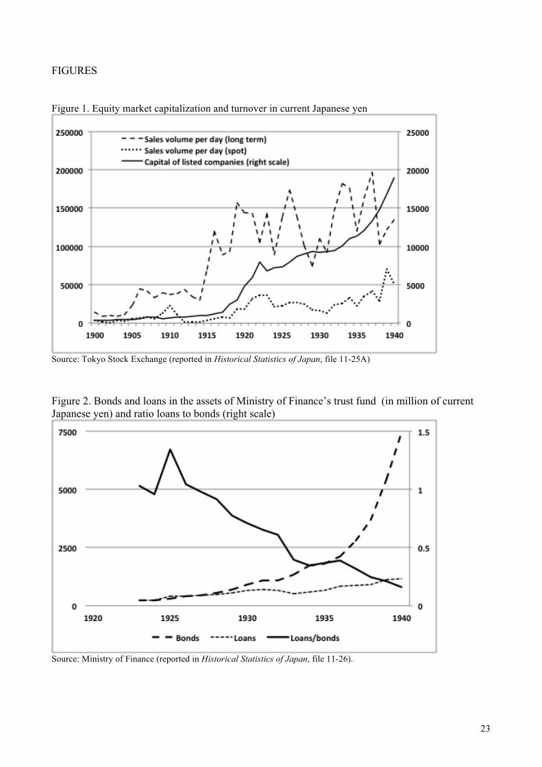
Figure 1. Equity market capitalization and turnover in current Japanese yen

Source: Tokyo Stock Exchange (reported in Historical Statistics of Japan, file 11-25A) Figure 2. Bonds and loans in the assets of Ministry of Finance’s trust fund (in million of current Japanese yen) and ratio loans to bonds (right scale)

Source: Ministry of Finance (reported in Historical Statistics of Japan, file 11-26).

! 24

Figure 3. Outstanding bonds at end of year (in million of current Japanese yen)

Source: Data of Bond Underwriters Association (reported in Historical Statistics of Japan, file 11-13).

! 25

Figure 4: Generalized Impulse Response Functions

-.001

.000

.001

.002

.003

.004

.005

.006

1 2 3 4 5 6 7 8 9 10

Response of RETINDUS to RETBOND

-.001

.000

.001

.002

.003

.004

.005

.006

1 2 3 4 5 6 7 8 9 10

Response of RETINDUS to RETUTI

Response to Generalized One S.D. Innovations ± 2 S.E.

-.0002

.0000

.0002

.0004

.0006

.0008

1 2 3 4 5 6 7 8 9 10

Response of RETBOND to RETINDUS

-.0002

.0000

.0002

.0004

.0006

.0008

1 2 3 4 5 6 7 8 9 10

Response of RETBOND to RETUTI

Response to Generalized One S.D. Innovations ± 2 S.E.

-.0005

.0000

.0005

.0010

.0015

.0020

.0025

1 2 3 4 5 6 7 8 9 10

Response of RETUTI to RETBOND

-.0005

.0000

.0005

.0010

.0015

.0020

.0025

1 2 3 4 5 6 7 8 9 10

Response of RETUTI to RETINDUS

Response to Cholesky One S.D. Innovations ± 2 S.E.

! 26

TABLES

Table 1. Descriptive statistics of TSE daily series

Industrials Utilities Bonds Mean 0.000312 7.63E-05 7.28E-05 Median 0 0 0 Maximum 0.115069 0.063716 0.017382 Minimum -0.059547 -0.034729 -0.019689 Std. Dev. 0.00925 0.004299 0.001936 Skewness 1.516052 0.905465 -0.459048 Kurtosis 28.71567 34.91172 22.72522 Jarque-Bera 60064.65 101354.9 38651.55 Probability 0 0 0 Sharpe ratio 0.03372973 0.01774831 0.0376033 Sum 0.670076 0.181557 0.17324 Sum Sq. Dev. 0.183888 0.043994 0.008914 Observations 2150 2381 2379

Table 2. Non-parametric variance ratio analysis

Industrials Utilities Bonds Block length R1 R2 R1 R2 R1 R2 k=2 6.686** 6.220** 10.651** 10.849** 4.683** 3.705** k=5 4.341** 4.186** 15.061** 14.895** 4.924** 4.334** k=10 3.910** 3.534** 15.979** 15.435** 4.084** 3.794** Bootstrapped critical values k=2 k=5 k=10 R1 R2 R1 R2 R1 R2 0.5% -2.615 -2.509 -2.734 -2.615 -2.358 -2.471 5% -1.580 -1.656 -1.610 -1.640 -1.702 -1.691 95% 1.662 1.742 1.634 1.642 1.544 1.884 99.5% 2.856 2.731 2.747 2.792 2.608 2.648

! 27

Table 3 Variable moving average (VMA) technical trading analysis

Panel A Industrials N(buy) N(sell) Buy Sell Buy-Sell Buy-Buy and hold VMA(1,50) 501 501 0.0018 -0.0007 0.0025 0.0015

2.9192** 2.7260**

VMA(1,150) 477 477 0.0019 -0.0006 0.0026 0.0017

2.9737** 2.9462**

VMA(5,150) 204 203 0.0019 0.0012 0.0007 0.0016

0.3181 1.2206

VMA(1,200) 461 461 0.0020 -0.0007 0.0027 0.0017

3.0101** 3.0260**

VMA(2,200) 328 327 0.0017 0.0003 0.0014 0.0014

1.1289 1.7258

Panel B Utilities N(buy) N(sell) Buy Sell Buy-Sell Buy-Buy and hold VMA(1,50) 463 464 0.0012 -0.0009 0.0022 0.0012

4.7658** 3.5632**

VMA(1,150) 437 438 0.0014 -0.0010 0.0024 0.0014

5.0972** 4.0289**

VMA(5,150) 166 167 0.0039 -0.0026 0.0065 0.0038

4.4658** 3.7189**

VMA(1,200) 428 429 0.0016 -0.0008 0.0024 0.0016

5.1459** 4.5476**

VMA(1,200) 283 283 0.0034 -0.0022 0.0056 0.0033

7.1135** 5.7149**

Panel C Bonds N(buy) N(sell) Buy Sell Buy-Sell Buy-Buy and hold VMA(1,50) 457 456 0.00039 -0.00006 0.0004 0.0003

2.1752* 2.2659*

VMA(1,150) 441 440 0.00039 -0.00004 0.0004 0.0003

2.1551* 2.2507*

VMA(5,150) 184 183 0.00108 -0.00024 0.0013 0.0010

2.5772* 2.6589**

VMA(1,200) 421 420 0.00055 -0.00003 0.0006 0.0005

2.9689** 3.4835**

VMA(2,200) 291 290 0.00082 -0.00008 0.0009 0.0007

3.0996** 3.5946**

Note: For each market, we report the results for the various VMA rules. The first two columns gives the number of buy

and sell signal generated. The third and fourth column gives the average returns associated to buy and sell signal. The

fifth and sixth columns give the average difference in buy-sell and buy-buy and hold returns as and the associated test

statistic. (*) and (**) indicate significance at the 5% and 1% level, respectively.

! 28

Table 4. Identification of events (GARCH model; see appendix 2 for details)

Date of the break

Day of the week

Date of the event

Nature of the main event identified in the Toyo Keizai yearbook

Industrial 25/03/32 24/03/38 19/05/38 21/09/38 11/10/38 07/12/38 07/01/39

Friday Wednesday Thursday Thursday Tuesday Wednesday Saturday

24/03/32 18/03/38 a 18/05/38 19/09/38 07/10/38 06/12/38 05/01/39 b

Monetary policy: approval of exchange rate control Industrial policy: adoption of 5-year plan for Manchuria steel industry Trade policy: announcement of an adjustment of trade tariff for important commodities Economic planning: adoption of an allocation system for fertilizers Economic planning/trade policy: change in the cotton textile export system Economic planning: issuance of bonds by electric power companies approved Politics: formation of the Hiranuma cabinet

Utilities 30/01/31 03/03/32 11/06/32 08/07/32 09/12/39

Friday Monday Saturday Friday Saturday

28/01/31 02/03/32 11/06/32 06/07/32 07/12/39

Public finance: authorization for the use of the reserve fund for earthquake reconstruction Public finance: issuance of the 3rd 4.75% public bonds (10 million yen) Finance: Taiwan Bank and Chosen Bank announce a reduction of their interest rates Public finance: issuance of bonds by the Manchuria Railways Co. (50 million yen) Public finance: final 1940 budget including support package to industrial companies

Bonds 07/10/33 13/08/35 21/02/36 28/03/36 02/04/36 25/04/36 02/06/36 12/08/36 06/11/36 14/11/36 17/12/36 08/01/37 06/08/37 16/10/37 24/03/38 16/07/38 21/10/38 14/12/38 23/12/38

Saturday Tuesday Friday Saturday Thursday Saturday Thursday Tuesday Wednesday Thursday Saturday Thursday Friday Friday Wednesday Saturday Friday Wednesday Friday

03/10/33 12/08/35 17/02/36 28/03/36 c 02/04/36 24/04/36 01/06/36 12/08/36 02/11/36 11/11/36 17/12/36 07/01/37 05/08/37 15/10/37 18/03/38 a 15/07/38 20/10/38 13/12/38 23/12/38

Politics: inter-ministerial conference on defense, diplomacy, and public finance Politics: assassination of Tetsuzan Nagata, chief of Mobilization Section, Ministry of War Manchuria: Proposal to USSR to establish a joint commission to settle border dispute. Politics: announcement of the names of the persons involved in the “February 26 incident” Finance: Bank of Japan suspends sale of 4% interest public bonds (d). Politics: first meeting of the inter-ministerial commission on international relations (e). Public finance: issuance of 3.5% public bonds (413 million yen; maturity on June 1949. Finance: approval of the fund of the Chamber of Commerce. Public finance: issuance of y public bonds by Manchuria approved (10 million yen) Military: “Takase incident” in Shanghai (f) Politics: decision to abandon accusation against Bonosuke Hisahara (February 26 incident) Monetary policy: introduction of capital controls by the Ministry of Finance. Monetary policy: introduction of capital controls by the Kwangtung Army (in Manchuria). Finance: decision to reduce to less than 10% the dividends served by insurance companies. Industrial policy: adoption of 5-year plan for Manchuria steel industry Public finance: use of part of the reserve funds for import of raw materials. Trade policy: reinforcement of export control for textile products. Issuance of public bonds (400 million yen). Finance: announcement of a new banking law.

Notes: (a) Bank holiday on 22 and 23/03/1938; (b) Bank holiday on 5/01/39; (c) “February 26 incident”: attempted coup d’état from February 26 to 28; (d) according to information reported in Toyo Keizai yearbook, decision made to prevent transactions on the futures market; (e) three ministries involved: War, Navy, and Foreign Affairs. (f) Assassination in Shanghai of Yasuji Takase, crew of a Japanese merchant vessel.

! 29

Table 5. Granger causality analysis

Dependent variable: RETINDUS

Excluded Chi-sq Df Prob.

RETBOND 19.306 8 0.013(*)

RETUTI 54.332 8 0.000(**)

All 77.636 16 0.000(**)

Dependent variable: RETBOND


RETINDUS 23.048 8 0.003(**)

RETUTI 13.029 8 0.110

All 52.106 16 0.000(**)

Dependent variable: RETUTI


RETINDUS 126.611 8 0.000(**)

RETBOND 16.022 8 0.042(*)

All 150.122 16 0.000(**)

! 30

Table 6. Variance decomposition analysis

Variance Decomposition of RETBOND:

Period S.E. RETBOND RETUTI RETINDUS

1 0.002298 96.472 1.961 1.566

2 0.002317 95.854 2.087 2.057

3 0.002322 95.524 2.227 2.248

4 0.002324 95.461 2.257 2.281

5 0.002325 95.458 2.259 2.282

6 0.002325 95.458 2.259 2.282

7 0.002325 95.456 2.260 2.282

8 0.002325 95.456 2.260 2.282

9 0.002325 95.456 2.2601 2.282

10 0.002325 95.456 2.2601 2.282

Variance Decomposition of RETUTI:


1 0.004585 1.737 89.122 9.139

2 0.004681 1.923 86.019 12.056

3 0.004723 1.949 85.170 12.880

4 0.004739 2.125 84.968 12.906

5 0.00474 2.125 84.947 12.926

6 0.00474 2.125 84.942 12.931

7 0.00474 2.126 84.941 12.931

8 0.00474 2.126 84.941 12.931

9 0.00474 2.126 84.941 12.931

10 0.00474 2.126 84.941 12.931

Variance Decomposition of RETINDUS:


1 0.010381 2.574 14.002 83.423

2 0.010487 2.651 15.399 81.949

3 0.010497 2.823 15.373 81.803

4 0.010502 2.851 15.405 81.743

5 0.010503 2.852 15.410 81.736

6 0.010503 2.853 15.410 81.735

7 0.010503 2.853 15.411 81.735

8 0.010503 2.853 15.411 81.735

9 0.010503 2.853 15.411 81.735

10 0.010503 2.853 15.411 81.735

Note: This table shows results from a Variance Decomposition Analysis following the method of Habsbrouck (1995).

! 31

APPENDICES

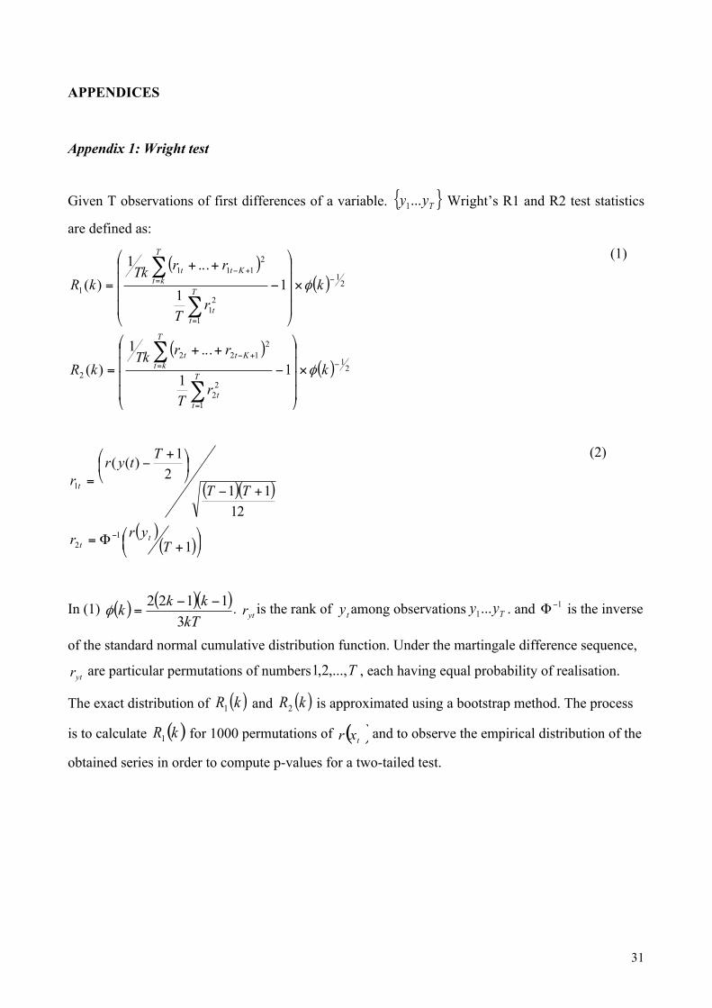
Appendix 1: Wright test

Given T observations of first differences of a variable. { }Tyy ...1 Wright’s R1 and R2 test statistics

are defined as:

( )( )

( )( ) 2

1

1

22

2122

2

21

1

21

2111

1

11

...1)(

11

...1)(

!

=

=+!

!

=

=+!

"

####

$

%

&&&&

'

(

!++

=

"

####

$

%

&&&&

'

(

!++

=

)

)

)

)

kr

T

rrTkkR

kr

T

rrTkkR

T

tt

T

ktKtt

T

tt

T

ktKtt

*

*

(1)

( )( )

( )( )!"

#$%&

+'=

+(

!"

#$%

& +(

=

(

1

1211

21)((

12

1

Tyrr

TT

Ttyrr

tt

t

(2)

In (1) ( ) ( )( )kTkkk

31122 !!

=" . ytr is the rank of ty among observations Tyy ...1 . and 1!" is the inverse

of the standard normal cumulative distribution function. Under the martingale difference sequence,

ytr are particular permutations of numbers T,...,2,1 , each having equal probability of realisation.

The exact distribution of ( )kR1 and ( )kR2 is approximated using a bootstrap method. The process

is to calculate ( )kR1 for 1000 permutations of ( )txr and to observe the empirical distribution of the

obtained series in order to compute p-values for a two-tailed test.

! 32

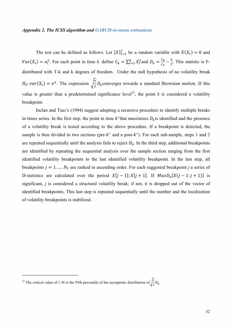
Appendix 2. The ICSS algorithm and GARCH-in-mean estimations

!

The test can be defined as follows. Let ! !!!! be a random variable with ! !! ! ! and

!"# !! ! !!!. For each point in time k. define !! ! !!!!!!! and !! ! !!

!!! !

!. This statistic is F-

distributed with T-k and k degrees of freedom. Under the null hypothesis of no volatility break

!!! !"# !! ! !!. The expression !!!!converges towards a standard Brownian motion. If this

value is greater than a predetermined significance level22, the point k is considered a volatility

breakpoint.

Inclan and Tiao’s (1994) suggest adopting a recursive procedure to identify multiple breaks

in times series. In the first step. the point in time !!that maximizes !!is identified and the presence

of a volatility break is tested according to the above procedure. If a breakpoint is detected, the

sample is then divided in two sections (pre-!! and a post-!!). For each sub-sample, steps 1 and 2

are repeated sequentially until the analysis fails to reject !!. In the third step, additional breakpoints

are identified by repeating the sequential analysis over the sample section ranging from the first

identified volatility breakpoints to the last identified volatility breakpoint. In the last step, all

breakpoints ! ! !!! !!! are ranked in ascending order. For each suggested breakpoint j a series of

D-statistics are calculated over the period ! ! ! ! !! ! ! ! . If !"#!! ! ! ! !! ! ! ! is

significant, j is considered a structural volatility break; if not, it is dropped out of the vector of

identified breakpoints. This last step is repeated sequentially until the number and the localization

of volatility breakpoints is stabilized.

! !

!!!!!!!!!!!!!!!!!!!!!!!!!!!!!!!!!!!!!!!!!!!!!!!!!!!!!!!!!!!!!22 The critical value of 1.36 is the 95th percentile of the asymptotic distribution of !

!!!.

! 33

!

Table A2. Identifying ARCH effects

Coefficients

P-value ARCH LM

Bonds

Bonds(-1) -.0404419* 0.049 350.961***

Constant .0000759 0.056 0

Utilities

Utilities(-1) .1567876** 0.000 144.587***

Constant .0000637 0.465 0

Industrials

Industrials(-1) .044183* 0.041 203.225***

Constant .0003021 0.130 0

Table A3. ADF test for stationarity

Industrial Utilities Bonds

Panel 1: Log(price)

C/T -1.511 -1.380 -1.714

C/D -2.229(*) -1.813(*) -2.096(*)

Panel 2: Dif(logprice)

C/T

-

36.651(**) -36.683(**) -39.756(**)

C/D

-

36.600(**) -36.660(**) -39.729 (**) Note: This table presents results for the KPSS test with a constant and a trend (C/T) and with a constant and a drift

(C/T) using data on prices and logarithmic returns. 5% and 1% critical values are-3.960 and -3.410 for the test including

a constant and a trend; and -2.328 and -1.645 for the test including a constant and a drift (**) and (*) indicate that the

null hypothesis of a unit root is rejected at the 1% and 5% levels, respectively.

! 34

Table A4. GARCH-in-mean estimations PANEL A:

without dummies Constant Constant Q(16) Skewness Kurtosis

INDUSTRIALS 0 0.058** 0.07 0.00*** 0.785*** 0.216*** 1.001 4.4812 0.273 19.99

0.74 0.02 0.14 0 0 0

UTILITIES 0.00* 0.159*** 0.139** 0.00*** 0.657*** 0.245*** 0.902 50.562 -1.402 20.28

0.07 0 0.01 0 0 0

BONDS 0 0.072*** 0.03 0.00*** 0.292*** 0.676*** 0.968 50.433 -0.625 30.74

0.3 0 0.52 0 0 0

PANEL B:

with all dummies

INDUSTRIALS -0.004 0.022 0.366 0.00*** 0.554*** 0.147*** 0.701 17.841 0.728 19.190

0.193 0.629 0.112 0 0 0

UTILITIES -0.002*** 0.154*** 0.346*** 0.000*** 0.581*** 0.149*** 0.73 54.07 0.052 25.104

0.01 0 0.006 0 0 0

BONDS 0 -0.042 -0.076 0.000*** 0.598*** 0.150*** 0.748 52.287 -0.012 16.06

0.26 0.311 0.387 0 0 0

PANEL C:

with significant dummies

INDUSTRIALS -0.004*** 0.024 0.376*** 0.000*** 0.557*** 0.151*** 0.708 16.266 0.741 19.389

0.001 0.592 0 0 0 0

UTILITIES -0.002*** 0.164*** 0.351*** 0.000*** 0.590*** 0.169*** 0.76 55.72 -0.539 21.224

0.003 0 0.004 0 0 0

BONDS 0 -0.042 -0.076 0.000*** 0.598*** 0.150*** 0.748 52.563 -0.101 16.568

0.617 0.305 0.687 0 0 0

Note: ** Significant above 5% level. Q(16) is the Ljung-Box Q-statistic for the 16th order

! 35

Table A5. Volatility breakpoints detected by the ICSS algorithm and GARCH model

Daily Index ICSS breaks (Filtered data) Significant dummies (GARCH model) Industrial 25/03/32

30/03/32 28/06/32 05/07/32 27/07/34 17/03/38 24/03/38 19/05/38 15/09/38 21/09/38 11/10/38 26/10/38 05/11/38 07/12/38 07/01/39 06/09/39 08/11/39

25/03/32 24/03/38 19/05/38 21/09/38 11/10/38 07/12/38 07/01/39

Utilities 30/01/31 27/01/32 30/01/32 23/02/32 03/03/32 08/04/32 15/04/32 11/06/32 08/07/32 29/08/33 10/04/34 16/10/34 02/11/34 10/03/38 12/04/38 14/04/38 05/11/38 31/01/39 12/04/39 09/12/39

30/01/31 03/03/32 11/06/32 08/07/32 09/12/39

Bonds 07/10/33 13/08/35 21/02/36 28/03/36 02/04/36 25/04/36 02/06/36 12/08/36 06/11/36 14/11/36 17/12/36 08/01/37 30/07/37 06/08/37 16/10/37 29/12/37 24/03/38 26/03/38 16/07/38 21/10/38 14/12/38 23/12/38 20/09/39

07/10/33 13/08/35 21/02/36 28/03/36 02/04/36 25/04/36 02/06/36 12/08/36 06/11/36 14/11/36 17/12/36 08/01/37 06/08/37 16/10/37 24/03/38 16/07/38 21/10/38 14/12/38 23/12/38

! 36

Figure A1: Daily returns (industrials)

Figure A2: Daily returns (utilities)

Figure A3: Daily returns (bonds)

-.05

0.05

.1.15

Indus

trial s

tocks

01 Jul 31 01 Jul 34 01 Jul 37 01 Jul 40Date

-.04

-.02

0.02

.04.06

Utilit

ies st

ocks

01 Jul 31 01 Jul 34 01 Jul 37 01 Jul 40date

-.03

-.02

-.01

0.01

.02Bo

nds

01 Jul 31 01 Jul 34 01 Jul 37 01 Jul 40Date

! 37

Appendix 3. The SVAR model

Our approach may be summarized as follows. Consider the moving average form of the

reduced structural VAR model:

(2)

Where Xt is a vector of returns. L is the lag operator and A*(L) is a transformed matrix of

coefficients such as )()(* 1 LALA !"= , where ! is the matrix of contemporaneous parameters

and A(L) the initial matrix of VAR parameters. Following standard practice, we orthogonalize

structural innovations by setting a diagonal structure on the residuals’ variance-covariance

matrix. The remaining n(n-1)/2 identifying constraints are then set following a Cholesky

decomposition:

(3)

ttttt uuXLAX !1;)(* "#=+=

!!!

"

#

$$$

%

&

=!!!

"

#

$$$

%

&

!!!

"

#

$$$

%

&

3

2

1

3

2

1

3231

21

001001

eee

uuu

''

'

! 38

Appendix 4. The DCC GARCH model

We model the pattern of cross-market conditional dynamics based on the DCC

GARCH introduced by Engle and Sheppard (2002). This approach can be summarized as

follows. Consider the following vector stochastic process:

( )tt

tt

HNX

,0~!

!µ +=

(A1)

Where Xt=[X1t. X2t. X3t] is a vector of financial returns and "t the residuals from the filtered

time series with zero mean and variance covariance matrix { }itt hH = . Letting

{ }itt hdiagD = and !!!!

"

#

$$$$

%

&

=

1

1

1

,

,,

,,

ijttij

tijtij

tijtij

tR''

''

''

be the time-varying conditional correlation

matrix for "t. we have tttt DRDH = with each element of Ht being equal to hi.t if i=.j and

tijtjti hh ,2/1,

2/1, ! otherwise. The elements of Dt are defined as univariate GARCH(1.1) processes

such as:

121 !! ++= itiitiiit hrh "#$ (A2)

In turn. the dynamic covariance structure also follows a GARCH pattern so that:

( ) ( )( ) ( )!"

!#$

><+++%%=

&&=

%%%

%%

0,;1'1 111

2/12/1

'('('('( tttt

NttNtt

QzzQQIQQIQR

(A3)

Where ! denotes the elementwise product of two matrices. Q is a sample covariance matrix

of "t. and ( )tt RNz ,0~ are standardized residuals from the univariate GARCH model. Note

that the correlation process is driven by two parameters ! and " which represent the impact of

shocks and lagged conditional correlation on contemporaneous correlations. respectively.

Estimation is conducted by decomposing the log likelihood function into a volatility

component and a correlation component. Univariate GARCH(1.1) volatility parameters are

thus first estimated for each the analyzed series. yielding series of standardized residuals. The

! 39

latter are used to derive a time-varying correlation matrix via maximum likelihood. Details on

the estimation procedure can be found Engle and Sheppard (2002).

Inspection of figure suggests no trend towards integration for the three markets under

scrutiny over the study period. However, it appears that the two stock markets display a

significantly higher correlation with each other (around 0.6) than with the bond market

(around 0.2). It should also be noted that correlations sometimes increase abruptly for

particular days. This echoes results from the ICSS analysis and suggests the existence of short

run spillovers between markets. However, the bond market appears segmented from the

utilities and industrials stock market.

Figure A4. Cross-market conditional correlation coefficient. 1931-1940

Note: this figure plots bivariate time-varying correlation coefficients as estimated from a DCC GARCH model.

"#$%!

"#$&!

"#$'!

"()"*+!

#$'!

#$&!

#$%!

#$,!

*!

*-(*! *-('! *-((! *-(&! *-(+! *-(%! *-(.! *-(,! *-(-! *-&#!

/012345673"89:6973! /012345673";<013! 89:6973";<013!

centre for economic history the …! 1 trading patterns at the tokyo stock exchange, 1931-1940...

Documents