central composite design application in oil agglomeration
TRANSCRIPT
http://dx.doi.org/10.5277/ppmp170230
Physicochem. Probl. Miner. Process. 53(1), 2017, 1061−1078 Physicochemical Problems
of Mineral Processing
www.minproc.pwr.wroc.pl/journal/ ISSN 1643-1049 (print)
ISSN 2084-4735 (online)
Received January 25, 2017; reviewed; accepted March 27, 2017
Central composite design application
in oil agglomeration of talc
Izabela Polowczyk, Tomasz Kozlecki
Wroclaw University of Science and Technology, Faculty of Chemistry, Division of Chemical Engineering,
Norwida 4/6, 50-373 Wroclaw, Poland. Corresponding author: [email protected] (I. Polowczyk)
Abstract: Talc has many applications in various branches of industry. This material is an inert one with a
naturally hydrophobic surface. Talc agglomeration is within the wide interest of pharmaceutical industry.
Oil agglomeration experiments of talc were carried out to find out and assess the significance of
experimental factors. Central composite design (CCD) was used to estimate the importance and
interrelation of the agglomeration process parameters. Four experimental factors have been evaluated, i.e.
concentration of cationic surfactant and oil, agitation intensity as well as time of the process. The median
size of agglomerates (D50) and the polydispersity span (PDI) were used as the process responses.
Logarithmic transformations of the responses provide better description of the model, than untransformed
responses, with the reduced cubic model for D50 and quadratic model for PDI. This was supported by the
Box-Cox plots. It was shown that there were many statistically important factors, including the
concentration of cationic surfactant and stirring rate for D50, concentration of oil and stirring rate for
PDI, as well as various interactions, up to third order for D50. Optimal conditions for minimum values of
reagent amounts as well as mixing time and intensity for the maximum size of agglomerates but of rather
narrow size distribution were found.
Keywords: talc, oil agglomeration, optimization, central composite design, design of experiment
Introduction
Talc is a magnesium silicate mineral which usually occurs in either foliated, granular
or fibrous forms. It is commonly used as a filler and a coating agent in paints,
lubricants, plastics, cosmetics, pharmaceuticals and ceramics manufacture. It is also
applied as a nucleating agent in plastic foaming processes (Wong and Park, 2012).
This substance is an inert one with a naturally hydrophobic surface (Bremmell and
Addai-Mensah, 2005). The pharmaceutical industry is one of the branch, where
agglomeration of talc is an interesting issue (Jadhav et al., 2011).
Oil agglomeration is a size enlargement method that facilitates separation
operations of solid processing (filtration, flotation, sedimentation) (Ennis, 1996). The
I. Polowczyk, T. Kozlecki 1062
main advantages making this method interesting for industrial applications (e.g.
pharmaceutics, pigments, and pesticides) are: high selectivity, possibility of fine
particles aggregation (below 5 μm) and simple equipment (Pietsch, 1991; House and
Veal, 1992; Huang and Berg, 2003). Oil agglomeration mostly depends on surface
properties of particles and oil/water interface (Drzymala, 2007; Bastrzyk et al., 2011;
Bastrzyk et al., 2012). In this process, an addition of an immiscible liquid (binder) to a
solid aqueous suspension causes adhesion of hydrophobic particles by capillary
interfacial forces (Rossetti and Simons, 2003; Negreiros et al., 2015). In the
suspension, between these hydrophobic particles liquid bridges are formed, which are
responsible for the mechanical strength and stability of agglomerates obtained,
whereas, the hydrophilic particles remain un-agglomerated (Sonmez and Cebeci,
2003). Literature data show that the several other factors affected the course of oil
agglomeration, which include the oil amount and type, particle size, agitation rate and
time, pH, and surfactant concentration (Sadowski, 1995; Aktas, 2002; Sonmez and
Cebeci, 2003; Duzyol and Ozkan, 2010; Bastrzyk et al., 2011; Bastrzyk et al., 2012;
Duzyol and Ozkan, 2014; Duzyol, 2015).
Success of oil agglomeration depends on selection of suitable operating parameters
(Balakin et al., 2015). Therefore, it is very important to determine the operating
parameters at which the responses reach their optimum.
The best known method for determining the important operating parameters for
agglomeration is to carry out experiments by changing one parameter and keeping the
others at a constant level. However, this one-variable-at-a-time technique does not
include interactive effects of parameters, and does not depict the exact effects of
various parameters on the process (Chary and Dastidar, 2013; Aslan and Unal, 2011;
Aslan, 2013). In order to avoid this, optimization studies using design of experiments
are of great importance.
Currently, numerous experimental designs are used. The most important first-order
designs are: 2𝑛 factorial, where n is the number of control variables (Montgomery,
2001), and the Plackett-Burman design (Plackett and Burman, 1946). The most
important second-order models are: central composite (CCD) (Box and Wilson, 1951)
and Box-Behnken three-level design (Box and Behnken, 1960). In the literature, a
number of useful design or techniques can be found to optimize the parameters for oil
agglomeration. It can be listed as the Taguchi method (Chary and Dastidar, 2010;
Kumar et al., 2015), response surface methodology (RSM) (Cebeci and Sonmez,
2006; Aslan and Unal, 2009; Aslan and Unal, 2011) and grey relational analysis
(GRA) (Aslan, 2013).
Central composite design (CCD) is an experimental design affiliated to response
the surface methodology (Liu et al., 2011). This method provides graphs rendering
and including the expanded center points (Oney and Tanriverdi, 2012). Results
obtained from the experiments in the light of the experimental design are defined as a
function of factors. Several polynomial models are used to create the model equation.
These polynomials show how the response of the system parameter values obtained
Central composite design application in oil agglomeration of talc 1063
effect at the same time (Oney and Tanriverdi, 2012). CCD is ideal for sequential
experimentation and allows a reasonable amount of information for testing lack of fit,
while not involving an unusually large number of design points (Demirel and Kayan,
2012). The central composite design has found an application for optimization of
chemical processes such as textile dye degradation (Demirel and Kayan, 2012),
removal of dyes (Azami et al., 2012; Azami et al., 2013), flocculation and coagulation
of wastewater (Fendri et al., 2013) and extraction of protein from wastewater
(Ramyadevi et al., 2012). However, until now, there is no information reported on
optimization of oil agglomeration of solid particles using CCD.
In this study, the importance of process parameters in oil agglomeration of talc was
evaluated using the central composite design. The surface active agent and bridging oil
concentrations together with the agitation intensity and process time were evaluated
experimental factors. The median size of agglomerates (D50) and the particle size
distribution span (PDI) were the process responses.
Materials and methods
A talc powder was purchased from LG Olsztyn (Poland) and originated from IMI Fabi
LLC (USA). This mineral sample was used as obtained and was of a pharmaceutical
grade and, according to supplier information, conformed to the requirements of
Pharmacopea. The average particle diameter of talc, determined using Mastersizer 2000
(Malvern), a laser diffraction instrument, was 9.5 µm. The BET surface area of the
powder determined by FlowSorb 2300 II instrument (Micromeritics) was 4.8 m2 g-1.
Oil agglomeration tests were carried out in a glass vessel (250 cm3 with an inner
diameter of 60 mm). A sample of 5 grams of talc together with 100 cm3 of distilled
water was intensively stirred by using the IKA EUROSTAR power control-visc 6000
overhead mechanical stirrer equipped with a 3-bladed propeller. The products of
agglomeration were separated and dried, and then subjected to the image analysis. The
procedure was as follows. Photographs were taken using the AxioImager M1m
microscope (Zeiss), operating in the transmitted light mode, and 8 bit grayscale
pictures were collected. Using ImagePro Plus ver. 6.0 software (Media Cybernetics),
histogram-based segmentation with 33 mesh was applied, resulting in white-on-black
image, which was analysed automatically in respect to the mean diameter, counting
bright objects. Because, in some cases, particles were bridged, an automatic watershed
split was applied. Measurement data were transferred to MS-Excel, and the median
size and PDI were calculated.
Oil agglomeration of talc proceeds irregularly without surfactant addition because
of the properties of talc surface. The cationic surfactant dodecylammonium
hydrochloride (DDAHCl) (POCh) was applied as a wetting agent and an emulsifier,
while kerosene (Sigma-Aldrich) was used as a bridging oil (Kelebek et al., 2008;
Bastrzyk et al., 2011; Polowczyk et al., 2014).
I. Polowczyk, T. Kozlecki 1064
Central composite design (CCD) was used to estimate the importance of the
agglomeration process parameters. The median size of agglomerates (D50) and particle
size span (PDI) were the process responses. Data were analyzed using a demo version
of Stat-Ease 10.0.5 software (Design Expert).
Results and discussion
Response surface methodology (RSM) is a set of statistical methods for empirical
model building (Box and Draper, 1987;; Montgomery, 2001; Khuri and
Mukhopadhyay, 2010). Using design of experiment (DoE) techniques, output
variables (responses) can be optimized in respect to input variables. An experiment
consists of several runs, with varying input variables, in order to identify and quantify
changes in output responses. Usually, such relationship can be approximated by low
level polynomial:
𝑦 = 𝑓(𝑥)𝛽 + 𝜖 (1)
where 𝑦 is a response of interest, 𝑥 = (𝑥1, 𝑥2, … , 𝑥𝑛) is the set of input variables, 𝑛 is
the number of variables, 𝑓(𝑥) is a vector function consisting of powers and cross-
products of powers of 𝑥1, 𝑥2, … , 𝑥𝑛, up to a certain degree (usually 1 or 2), 𝛽 is a
vector of unknown constant coefficients, called parameters, and 𝜖 is a random
experimental error. The surface represented by 𝑓(𝑥)𝛽 is called a response surface.
There are two most important models used in RSM, that is first and second degree.
The former one is represented by equation (Khuri and Mukhopadhyay, 2010):
𝑦 = 𝛽0 + ∑ 𝛽𝑖𝑥𝑖 + 𝜖𝑛𝑖=1 (2)
where 𝛽𝑖 are the linear coefficients and 𝛽0 is an intercept. Second order model is
described by the following equation:
𝑦 = 𝛽0 + ∑ 𝛽𝑖𝑥𝑖 + ∑ 𝛽𝑖𝑗𝑥𝑖𝑥𝑗 + ∑ 𝛽𝑖𝑖𝑥𝑖2𝑛
𝑖=11≤𝑖<𝑗≤𝑛𝑛𝑖=1 + 𝜖 (3)
where 𝛽𝑖𝑗 are called cross-product coefficients, and 𝛽𝑖𝑖 are quadratic coefficients.
Sometimes ∑ 𝛽𝑖𝑖𝑥𝑖2𝑛
𝑖=1 term is omitted from the model, which is then called 2-factor
interaction (2FI). When complete equation (3) is employed, the model is called either
full quadratic or simply quadratic. Sometimes, third level (cubic) equation is also
used. Such cubic model is usually too complicated, and there is a potential risk of
aliasing, i.e. when estimate of effect also includes the influence of either one or more
other effects, usually high-order interactions. Aliasing does not need to confound
whole model, because such higher order interaction is often non-existent or
insignificant (Antony, 2003).
Frequently used in the industrial applications as well as in scientific research,
central composite design (CCD) was selected in this study. Generally, CCD can be

Central composite design application in oil agglomeration of talc 1065
described as 2𝑛 factorial design with additional central and axial points, allowing
calculating parameters of a second-order model. It involves 2𝑛 factorial points, 2𝑛
axial points and one central point. Usually axial and/or central points are replicated.
Axial points are placed at the distance 𝛼 from the design center, thus CCD uses five
levels of parameters:+𝛼, +1, 0, −1, −𝛼. The value of 𝛼 is usually chosen to make
design either orthogonal or rotatable (Draper, 2008). The experimental design is
orthogonal if the effects of any factor sum to zero across the effects of the other
factors. The design is rotatable if the variance of the predicted response at any point 𝑥
depends only on the distance of 𝑥 from the center point. Rotatability is achieved when:
𝛼 = √2𝑛4 . (4)
The design studied in the current contribution consisted of four experimental
factors, that is DDAHCl-to-talc mass ratio (A), kerosene-to-talc mass ratio (B),
stirring time (C) and stirring rate (D). For 4 factors, in order to achieve rotatability,
according to equation (4), the value of 𝛼 should be equal to 2. Unfortunately, this
resulted in negative values of parameters A and C at – 𝛼 level, thus we set 𝛼 = √2. We decided to skip parameter coding and the actual values were used instead. The
values of parameters are given in Table 1, and the summary of the design in Table 2.
Table 1. Experimental factors
Level
Parameter Unit Label – –1 0 +1 +
DDAHCl-to-talc mg g-1 A 1.31 1.60 2.30 3.00 3.28
Kerosene-to-talc g g-1 B 0.38 0.48 0.72 0.96 1.06
Time min C 3.44 8 19 30 34.6
Stir rate rpm D 620 1200 2600 4000 4580
Table 2. Parameters of experimental design
Parameter Value
Design type Central composite
Process order 2FI/Quadratic/Cubic
Number of variables 4
Number of responses 2
Star distance () √𝟐
Replicates of factorial points 1
Replicates of star points 2
Center points 2
Total number of runs 34

I. Polowczyk, T. Kozlecki 1066
Table 3. Results of experimental runs
Run DDAHCl [mg g-1] Kerosene [g g-1] Time [min] Stir rate[rpm] 𝐷50 [mm] PDI
1 1.31 0.72 19.00 2600 0.079 3.14
2 1.31 0.72 19.00 2600 0.168 1.96
3 1.60 0.48 8.00 1200 0.052 2.82
4 1.60 0.48 30.00 1200 0.316 1.34
5 1.60 0.48 8.00 4000 0.093 1.4
6 1.60 0.48 30.00 4000 0.131 0.81
7 1.60 0.96 8.00 1200 0.135 4.47
8 1.60 0.96 30.00 1200 0.263 5.58
9 1.60 0.96 8.00 4000 0.135 3.39
10 1.60 0.96 30.00 4000 0.039 15.42
11 2.30 0.38 19.00 2600 0.171 0.59
12 2.30 0.38 19.00 2600 0.111 0.67
13 2.30 0.72 3.44 2600 0.191 3.04
14 2.30 0.72 3.44 2600 0.24 3.05
15 2.30 0.72 34.60 2600 0.399 1.41
16 2.30 0.72 34.60 2600 0.372 1.84
17 2.30 0.72 19.00 620 0.091 3.58
18 2.30 0.72 19.00 620 0.061 6.85
19 2.30 0.72 19.00 4580 0.159 1.03
20 2.30 0.72 19.00 4580 0.168 1.62
21 2.30 0.72 19.00 2600 0.657 1.22
22 2.30 0.72 19.00 2600 0.62 3.96
23 2.30 1.06 19.00 2600 0.097 4.64
24 2.30 1.06 19.00 2600 0.143 2.89
25 3.00 0.48 8.00 1200 0.144 6.8
26 3.00 0.48 30.00 1200 0.361 2.37
27 3.00 0.48 8.00 4000 0.199 0.58
28 3.00 0.48 30.00 4000 0.404 1.34
29 3.00 0.96 8.00 1200 0.292 5.74
30 3.00 0.96 30.00 1200 0.129 4.31
31 3.00 0.96 8.00 4000 0.193 1.24
32 3.00 0.96 30.00 4000 0.03 9.72
33 3.28 0.72 19.00 2600 0.605 3.77
34 3.28 0.72 19.00 2600 0.574 2.88
Two responses were analyzed: median particle size (D50) and particle size width
DPI defined as (Merkus, 2009):
PDI =𝐷90−𝐷10
𝐷50 (5)

Central composite design application in oil agglomeration of talc 1067
where D10 and D90 are first and last deciles (Sheskin, 2004) of particle size
distribution, respectively. This parameter, sometimes called span, is commonly
accepted as a measure of width of particle size distribution (Merkus, 2009). In
practice, in agglomeration processes a relatively uniform and narrow agglomerates
size distribution is requested for the granular product (Pietsch, 1991; 2005).
All runs were randomized in order to avoid systematic errors. The results are
shown in Table 3.
One can observe that the ratio of maximal to minimal response is, in both cases,
greater than 20. This suggests that some transformation should be applied. Base 10
logarithm was selected as the transformation function. This selection was supported by
the Box-Cox transformation (Box and Cox, 1964).
a) b)
Fig. 1. The Box-Cox plots of original data a) for D50 and b) for PDI
a) b)
Fig. 2. The Box-Cox plots of transformed data a) for D50 and b) for PDI
The Box-Cox plots obtained before and after logarithmic transformation by the
Design Expert software are shown in Figs. 1 and 2 for D50 and PDI, respectively a)
and b). Current lambda values were 1 for the original data (Fig. 1) and this value was
beyond the confidence intervals (C.I.). However, best value lambda was -0.07
showing the need of logarithmic transformation for the both parameters. After
transformation (Fig. 2), the lambda obtained was 0 and this value was very near to -
Design-Expert® Softw are
D50
Lambda
Current = 1
Best = -0.07
Low C.I. = -0.54
High C.I. = 0.44
Recommend transform:
Log
(Lambda = 0)
Lambda
Ln
(Re
sid
ua
lSS
)
Box-Cox Plot for Power Transforms
-1.91
-0.52
0.87
2.27
3.66
-3 -2 -1 0 1 2 3
Design-Expert® Softw are
PDI
Lambda
Current = 1
Best = -0.07
Low C.I. = -0.52
High C.I. = 0.37
Recommend transform:
Log
(Lambda = 0)
Lambda
Ln
(Re
sid
ua
lSS
)
Box-Cox Plot for Power Transforms
2.97
4.58
6.19
7.80
9.41
-3 -2 -1 0 1 2 3
Design-Expert® Softw are
Log10(D50)
Lambda
Current = 0
Best = -0.07
Low C.I. = -0.54
High C.I. = 0.44
Recommend transform:
Log
(Lambda = 0)
Lambda
Ln
(Re
sid
ua
lSS
)
Box-Cox Plot for Power Transforms
-1.91
-0.52
0.87
2.27
3.66
-3 -2 -1 0 1 2 3
Design-Expert® Softw are
Log10(PDI)
Lambda
Current = 0
Best = -0.07
Low C.I. = -0.52
High C.I. = 0.37
Recommend transform:
Log
(Lambda = 0)
Lambda
Ln
(Re
sid
ua
lSS
)
Box-Cox Plot for Power Transforms
2.97
4.58
6.19
7.80
9.41
-3 -2 -1 0 1 2 3
I. Polowczyk, T. Kozlecki 1068
0.07 and between the confidence intervals showing the efficiency of logarithmic
transformation.
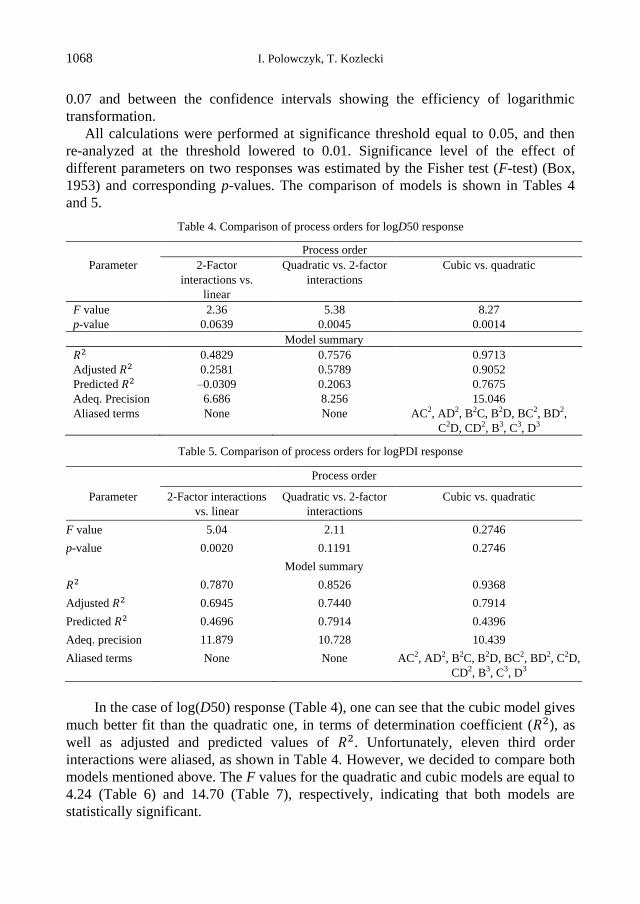
All calculations were performed at significance threshold equal to 0.05, and then
re-analyzed at the threshold lowered to 0.01. Significance level of the effect of
different parameters on two responses was estimated by the Fisher test (F-test) (Box,
1953) and corresponding p-values. The comparison of models is shown in Tables 4
and 5.
Table 4. Comparison of process orders for logD50 response
Process order
Parameter 2-Factor
interactions vs.
linear
Quadratic vs. 2-factor
interactions
Cubic vs. quadratic
F value 2.36 5.38 8.27
p-value 0.0639 0.0045 0.0014
Model summary
𝑅2 0.4829 0.7576 0.9713
Adjusted 𝑅2 0.2581 0.5789 0.9052
Predicted 𝑅2 –0.0309 0.2063 0.7675
Adeq. Precision 6.686 8.256 15.046
Aliased terms None None AC2, AD2, B2C, B2D, BC2, BD2,
C2D, CD2, B3, C3, D3
Table 5. Comparison of process orders for logPDI response
Process order
Parameter 2-Factor interactions
vs. linear
Quadratic vs. 2-factor
interactions
Cubic vs. quadratic
F value 5.04 2.11 0.2746
p-value 0.0020 0.1191 0.2746
Model summary
𝑅2 0.7870 0.8526 0.9368
Adjusted 𝑅2 0.6945 0.7440 0.7914
Predicted 𝑅2 0.4696 0.7914 0.4396
Adeq. precision 11.879 10.728 10.439
Aliased terms None None AC2, AD2, B2C, B2D, BC2, BD2, C2D,
CD2, B3, C3, D3
In the case of log(D50) response (Table 4), one can see that the cubic model gives
much better fit than the quadratic one, in terms of determination coefficient (𝑅2), as
well as adjusted and predicted values of 𝑅2. Unfortunately, eleven third order
interactions were aliased, as shown in Table 4. However, we decided to compare both
models mentioned above. The F values for the quadratic and cubic models are equal to
4.24 (Table 6) and 14.70 (Table 7), respectively, indicating that both models are
statistically significant.

Central composite design application in oil agglomeration of talc 1069
Table 6. ANOVA table for log(D50) – quadratic model
Source Sum of squares Degrees of
freedom
Mean square F value p-value
Prob > Fa
Model 2.8647 14 0.2046 4.2411 0.0021
A-DDAHCl 0.4779 1 0.4779 9.9052 0.0053
B-Kerosene 0.0943 1 0.0943 1.9543 0.1782
C-Time 0.0374 1 0.0374 0.7761 0.3893
D-Stir rate 0.0159 1 0.0159 0.3295 0.5727
AB 0.0981 1 0.0981 2.0328 0.1702
AC 0.0811 1 0.0811 1.6817 0.2102
AD 0.0070 1 0.0070 0.1453 0.7073
BC 0.5822 1 0.5822 12.0664 0.0025
BD 0.1810 1 0.1810 3.7508 0.0678
CD 0.2523 1 0.2523 5.2286 0.0339
A2 0.0065 1 0.0065 0.1354 0.7169
B2 0.4617 1 0.4617 9.5689 0.0060
C2 0.0000 1 0.0000 0.0000 0.9982
D2 0.6400 1 0.6400 13.2640 0.0017
Residual 0.9167 19 0.0482
Lack of Fit 0.8099 10 0.0810 6.8223 0.0040
Pure Error 0.1068 9 0.0119
Corr. Total 3.7814 33
a Statistically significant terms for significance threshold 0.05 are underlined.
The chance that F values were so high due to the noise which was equal to 0.21
and 0.01%, respectively. P-values less than 0.0500 indicate that the model terms are
significant. In the case of quadratic model (Table 6) A, BC, CD, B2, D2 were
significant model terms. Values greater than 0.1000 indicate that the model terms are
not significant. At more rigorous significance threshold equal to 0.01, CD term
became insignificant. The lack of fit F value of 6.82 implied that the lack of fit
was significant, which was unfavorable. The model fitting was expected. There was
only 0.40% chance that a lack of fit F-value this large could occur due to noise.
An adequate precision parameter value was 8.256 (Table 4). This indicated an
adequate signal, because for a good signal-to-noise ratio it should be greater than 4.
The predicted 𝑅2 of 0.2063 was much lower than adjusted 𝑅2 (0.5789). This might
indicate a large block effect or a possible problem with model and/or data. Therefore,
we decided to analyze the aliased cubic model, with manually removed confounded
terms.
Statistically significant terms at significance threshold 0.05 were identified to be,
starting from to least significant, according to the p-value, D2, B2, BC, A2D, CD, A3,
A, AB2, BD, A2, C2, D, AB, AC, and C. At significance threshold 0.01, several terms
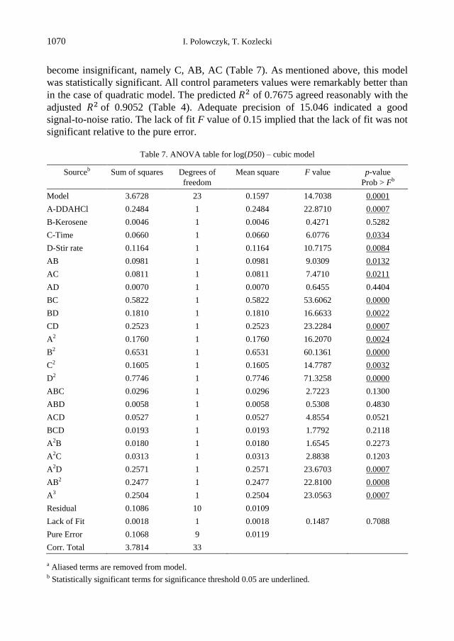
I. Polowczyk, T. Kozlecki 1070
become insignificant, namely C, AB, AC (Table 7). As mentioned above, this model
was statistically significant. All control parameters values were remarkably better than
in the case of quadratic model. The predicted 𝑅2 of 0.7675 agreed reasonably with the
adjusted 𝑅2 of 0.9052 (Table 4). Adequate precision of 15.046 indicated a good
signal-to-noise ratio. The lack of fit F value of 0.15 implied that the lack of fit was not
significant relative to the pure error.
Table 7. ANOVA table for log(D50) – cubic model
Sourceb Sum of squares Degrees of
freedom
Mean square F value p-value
Prob > Fb
Model 3.6728 23 0.1597 14.7038 0.0001
A-DDAHCl 0.2484 1 0.2484 22.8710 0.0007
B-Kerosene 0.0046 1 0.0046 0.4271 0.5282
C-Time 0.0660 1 0.0660 6.0776 0.0334
D-Stir rate 0.1164 1 0.1164 10.7175 0.0084
AB 0.0981 1 0.0981 9.0309 0.0132
AC 0.0811 1 0.0811 7.4710 0.0211
AD 0.0070 1 0.0070 0.6455 0.4404
BC 0.5822 1 0.5822 53.6062 0.0000
BD 0.1810 1 0.1810 16.6633 0.0022
CD 0.2523 1 0.2523 23.2284 0.0007
A2 0.1760 1 0.1760 16.2070 0.0024
B2 0.6531 1 0.6531 60.1361 0.0000
C2 0.1605 1 0.1605 14.7787 0.0032
D2 0.7746 1 0.7746 71.3258 0.0000
ABC 0.0296 1 0.0296 2.7223 0.1300
ABD 0.0058 1 0.0058 0.5308 0.4830
ACD 0.0527 1 0.0527 4.8554 0.0521
BCD 0.0193 1 0.0193 1.7792 0.2118
A2B 0.0180 1 0.0180 1.6545 0.2273
A2C 0.0313 1 0.0313 2.8838 0.1203
A2D 0.2571 1 0.2571 23.6703 0.0007
AB2 0.2477 1 0.2477 22.8100 0.0008
A3 0.2504 1 0.2504 23.0563 0.0007
Residual 0.1086 10 0.0109
Lack of Fit 0.0018 1 0.0018 0.1487 0.7088
Pure Error 0.1068 9 0.0119
Corr. Total 3.7814 33
a Aliased terms are removed from model. b Statistically significant terms for significance threshold 0.05 are underlined.
Central composite design application in oil agglomeration of talc 1071
Therefore, based on this observation, the median size of talc agglomerates is
affected mainly by the concentration of cationic surfactant DDAHCl as well as
intensity and, to a lesser extent, mixing time. The agglomerate size is controlled by the
balance between agglomerate interaction influenced by capillary forces and the
destructive forces determined by the shearing regime. The former are correlated with
the water and oil interfacial tension which is affected by the presence of surfactant.
Therefore, a quantity of surfactant added to the system is of importance for spherical
agglomeration since also affects the attachment of oil droplets to the mineral particle
surface and spreading on it (Laskowski and Yu, 2000). The presence of surfactant can
lower the strength of oil bridges, even to the point that agglomerates can be torn apart
by shear forces (Cebeci and Sönmez, 2004; Ozkan et al., 2005). Also, emulsification
by mixing of oil in the presence of surfactant lowers the amount of bridging liquid
necessary for agglomeration of mineral particles, due to the decrease of oil droplets
size (Laskowski and Yu, 2000). Therefore, depending on the mixing intensity and
bridging oil amount, the density and volume of the agglomerates can change. At
constant amount of oil added to predetermined amount of the suspension of particles
in water and subjected to mixing with constant intensity, the oil agglomeration process
takes place in four stages. In the first short stage, pendular oil floccules are formed. In
the second stage, so-called zero growth, a complete transition of emulsion droplets
into agglomerates is observed. As a consequence, third stage of a rapid growth of
aggregates is achieved. The last stage reflects final forming of agglomerates
(equilibrium period), which, at appropriately intensive mixing, can become either
spherical or form the sphere-like structure. Small decrease in the diameter of
agglomerates can be observed due to compression and forcing out water from the
structure of aggregates (Drzymala, 2007).
The equation in terms of actual factors can be employed to predict the response for
given levels of each factor. The logD50 response can be expressed by the polynomial
model. In the case of the cubic model, using coded factors, is as follows:
log(𝐷50) = −1825 + 1761𝐴 + 0.058𝐶 − 2.92 × 10⁻⁴𝐷 − 1098𝐴𝐵 + 0.059𝐴𝐶 +0.0057𝐵𝐶 + 4.77 × 10⁻⁴𝐵𝐷 − 1.36 × 10⁻⁵𝐶𝐷 − 634𝐴2 − 1764𝐵2 −0.00143𝐶2 − 1.94 × 10⁻⁷𝐷2 − 0.00032𝐴2𝐷 + 764.4𝐴𝐵2 + 92.18𝐴3. (6)
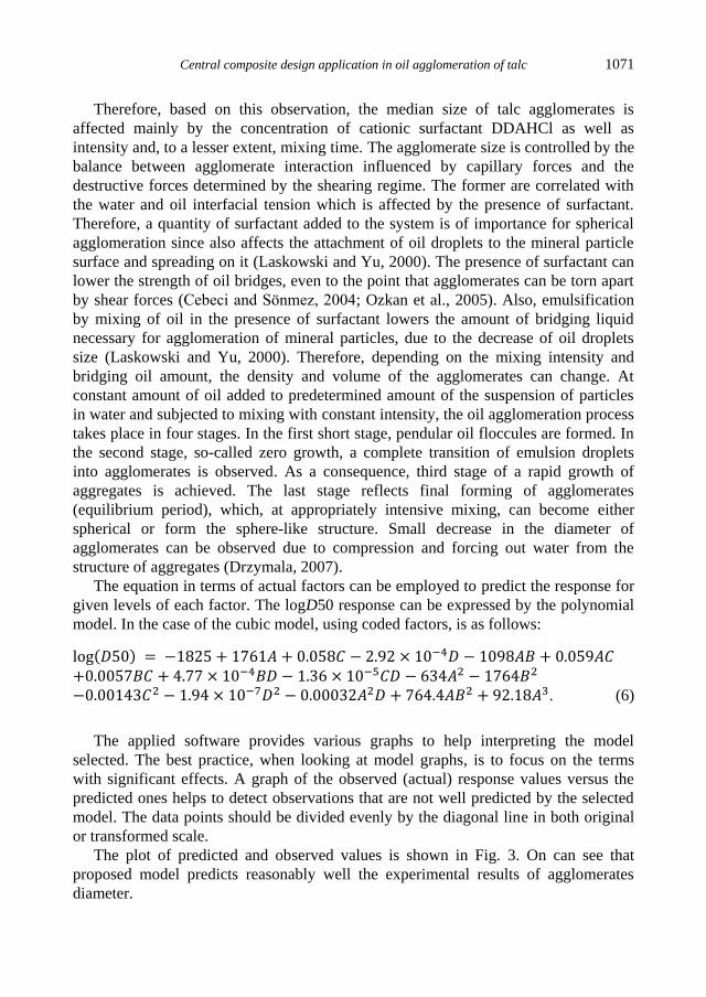
The applied software provides various graphs to help interpreting the model
selected. The best practice, when looking at model graphs, is to focus on the terms
with significant effects. A graph of the observed (actual) response values versus the
predicted ones helps to detect observations that are not well predicted by the selected
model. The data points should be divided evenly by the diagonal line in both original
or transformed scale.
The plot of predicted and observed values is shown in Fig. 3. On can see that
proposed model predicts reasonably well the experimental results of agglomerates
diameter.
I. Polowczyk, T. Kozlecki 1072
Fig. 3. Predicted vs. observed values of logD50 for cubic model, R2 = 0.7675
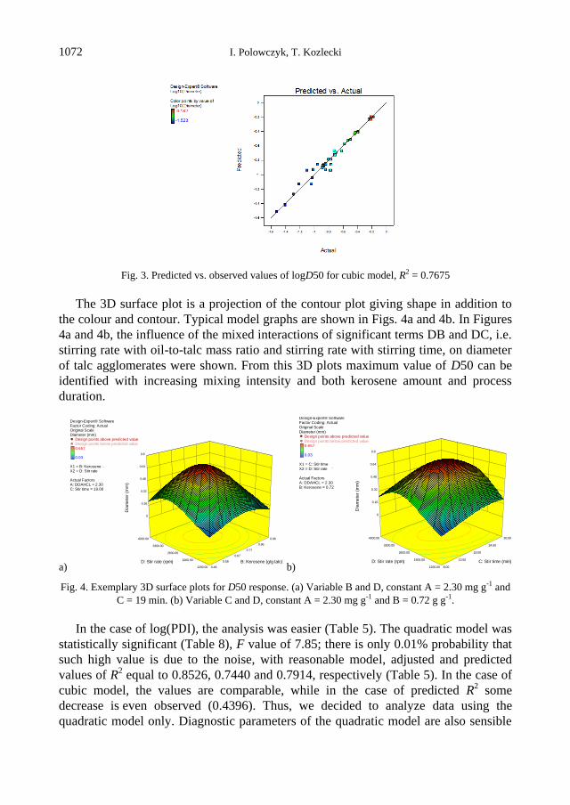
The 3D surface plot is a projection of the contour plot giving shape in addition to
the colour and contour. Typical model graphs are shown in Figs. 4a and 4b. In Figures
4a and 4b, the influence of the mixed interactions of significant terms DB and DC, i.e.
stirring rate with oil-to-talc mass ratio and stirring rate with stirring time, on diameter
of talc agglomerates were shown. From this 3D plots maximum value of D50 can be
identified with increasing mixing intensity and both kerosene amount and process
duration.
a) b)
Fig. 4. Exemplary 3D surface plots for D50 response. (a) Variable B and D, constant A = 2.30 mg g-1 and
C = 19 min. (b) Variable C and D, constant A = 2.30 mg g-1 and B = 0.72 g g-1.
In the case of log(PDI), the analysis was easier (Table 5). The quadratic model was
statistically significant (Table 8), F value of 7.85; there is only 0.01% probability that
such high value is due to the noise, with reasonable model, adjusted and predicted
values of R2 equal to 0.8526, 0.7440 and 0.7914, respectively (Table 5). In the case of
cubic model, the values are comparable, while in the case of predicted R2 some
decrease is even observed (0.4396). Thus, we decided to analyze data using the
quadratic model only. Diagnostic parameters of the quadratic model are also sensible
Design-Expert® SoftwareFactor Coding: ActualOriginal ScaleDiameter (mm)
Design points above predicted valueDesign points below predicted value0.657
0.03
X1 = B: KeroseneX2 = D: Stir rate
Actual FactorsA: DDAHCL = 2.30C: Stir time = 19.00
1200.00
1900.00
2600.00
3300.00
4000.00
0.48
0.58
0.67
0.77
0.86
0.96
0
0.16
0.32
0.48
0.64
0.8
Dia
mete
r (m
m)
B: Kerosene (g/g talc)D: Stir rate (rpm)
Design-Expert® SoftwareFactor Coding: ActualOriginal ScaleDiameter (mm)
Design points above predicted valueDesign points below predicted value0.657
0.03
X1 = C: Stir timeX2 = D: Stir rate
Actual FactorsA: DDAHCL = 2.30B: Kerosene = 0.72
1200.00
1900.00
2600.00
3300.00
4000.00
8.00
13.50
19.00
24.50
30.00
0
0.16
0.32
0.48
0.64
0.8
Dia
me
ter
(mm
)
C: Stir time (min)D: Stir rate (rpm)

Central composite design application in oil agglomeration of talc 1073
(Table 8). The lack of fit F-value of 1.24 implies the lack of fit is not significant
relative to the pure error. There is 37.84% chance that a lack of fit F-value this large
could occur due to the noise. Signal-to-noise of 10.687 (Table 5) is much higher
than 4, thus the signal is adequate. B, D, BC, BD, CD, A2 were identified as significant
model terms at threshold level of 0.05, while at threshold level of 0.01 BD and A2
became insignificant.
Table 8. ANOVA table for log(PDI) response - quadratic model
Source Sum of squares Degrees of
freedom
Mean square F value p-value
Prob > Fa
Model 3.3952 14 0.2425 7.8496 0.0000
A-DDAHCl 0.0014 1 0.0014 0.0456 0.8331
B-Kerosene 1.5124 1 1.5124 48.9516 0.0000
C-Time 0.0003 1 0.0003 0.0096 0.9230
D-Stir rate 0.5049 1 0.5049 16.3436 0.0007
AB 0.0765 1 0.0765 2.4772 0.1320
AC 0.0145 1 0.0145 0.4706 0.5010
AD 0.1274 1 0.1274 4.1231 0.0565
BC 0.2967 1 0.2967 9.6043 0.0059
BD 0.2136 1 0.2136 6.9125 0.0165
CD 0.3866 1 0.3866 12.5143 0.0022
A2 0.1425 1 0.1425 4.6112 0.0449
B2 0.0236 1 0.0236 0.7632 0.3932
C2 0.0262 1 0.0262 0.8483 0.3686
D2 0.0751 1 0.0751 2.4307 0.1355
Residual 0.5870 19 0.0309
Lack of Fit 0.3401 10 0.0340 1.2396 0.3784
Pure Error 0.2469 9 0.0274
Corr. Total 3.9822 33
a Statistically significant terms for significance threshold 0.05 are underlined.
It follows from above that amount of kerosene and stirring rate influence to the
greatest degree a span of the agglomerates size distribution of talc. The agglomeration
process may be considered as a collision between hydrophobic particle and
hydrophobic oil droplet. These collisions lead to adhesion as a result of the formation
of pendular oil bridges (Kawashima and Capes, 1974). Physical forms of agglomerates
are dependent on solid-oil-water interface properties, and, to a great extent, on amount
of oil and the hydrodynamics of the process, i.e. intensity and mixing time. There can
be identified three states of agglomerates: pendular, funicular, and capillary
(Drzymala, 2007). In the pendular state, oil bridges are formed between particles,
bringing them into aggregates in the predominant aqueous phase. Increasing the
I. Polowczyk, T. Kozlecki 1074
amount of oil, as well as intensive mixing, can result in the increased agglomerate
density. Consequently, the oil phase starts to dominate and water bridges are formed
in the aggregates (funicular state). In the capillary state, the particles are bound
together with oil only and there are no bridges. Further oil addition to the system
causes formation of a separate oil phase containing the particles (Drzymala, 2007).
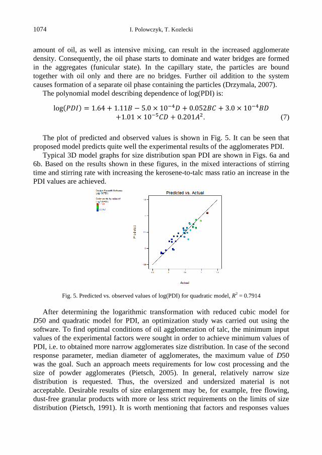
The polynomial model describing dependence of log(PDI) is:
log(𝑃𝐷𝐼) = 1.64 + 1.11𝐵 − 5.0 × 10⁻⁴𝐷 + 0.052𝐵𝐶 + 3.0 × 10⁻⁴𝐵𝐷 +1.01 × 10⁻⁵𝐶𝐷 + 0.201𝐴2. (7)
The plot of predicted and observed values is shown in Fig. 5. It can be seen that
proposed model predicts quite well the experimental results of the agglomerates PDI.
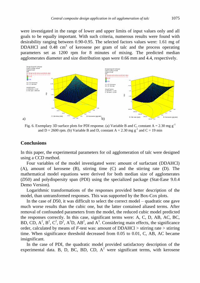
Typical 3D model graphs for size distribution span PDI are shown in Figs. 6a and
6b. Based on the results shown in these figures, in the mixed interactions of stirring
time and stirring rate with increasing the kerosene-to-talc mass ratio an increase in the
PDI values are achieved.
Fig. 5. Predicted vs. observed values of log(PDI) for quadratic model, R2 = 0.7914
After determining the logarithmic transformation with reduced cubic model for
D50 and quadratic model for PDI, an optimization study was carried out using the
software. To find optimal conditions of oil agglomeration of talc, the minimum input
values of the experimental factors were sought in order to achieve minimum values of
PDI, i.e. to obtained more narrow agglomerates size distribution. In case of the second
response parameter, median diameter of agglomerates, the maximum value of D50
was the goal. Such an approach meets requirements for low cost processing and the
size of powder agglomerates (Pietsch, 2005). In general, relatively narrow size
distribution is requested. Thus, the oversized and undersized material is not
acceptable. Desirable results of size enlargement may be, for example, free flowing,
dust-free granular products with more or less strict requirements on the limits of size
distribution (Pietsch, 1991). It is worth mentioning that factors and responses values
Central composite design application in oil agglomeration of talc 1075
were investigated in the range of lower and upper limits of input values only and all
goals to be equally important. With such criteria, numerous results were found with
desirability ranging between 0.90-0.95. The selected factors values were: 1.61 mg of
DDAHCl and 0.48 cm3 of kerosene per gram of talc and the process operating
parameters set as 1200 rpm for 8 minutes of mixing. The predicted median
agglomerates diameter and size distribution span were 0.66 mm and 4.4, respectively.
a) b)
Fig. 6. Exemplary 3D surface plots for PDI response. (a) Variable B and C, constant A = 2.30 mg g-1
and D = 2600 rpm. (b) Variable B and D, constant A = 2.30 mg g-1 and C = 19 min
Conclusions
In this paper, the experimental parameters for oil agglomeration of talc were designed
using a CCD method.
Four variables of the model investigated were: amount of surfactant (DDAHCl)
(A), amount of kerosene (B), stirring time (C) and the stirring rate (D). The
mathematical model equations were derived for both median size of agglomerates
(D50) and polydispersity span (PDI) using the specialized package (Stat-Ease 9.0.4
Demo Version).
Logarithmic transformations of the responses provided better description of the
model, than untransformed responses. This was supported by the Box-Cox plots.
In the case of D50, it was difficult to select the correct model – quadratic one gave
much worse results than the cubic one, but the latter contained aliased terms. After
removal of confounded parameters from the model, the reduced cubic model predicted
the responses correctly. In this case, significant terms were: A, C, D, AB, AC, BC,
BD, CD, A2, B2, C2, D2, A2D, AB2, and A3. Considering main effects, the significance
order, calculated by means of F-test was: amount of DDAHCl > stirring rate > stirring
time. When significance threshold decreased from 0.05 to 0.01, C, AB, AC became
insignificant.
In the case of PDI, the quadratic model provided satisfactory description of the
experimental data. B, D, BC, BD, CD, A2 were significant terms, with kerosene
Design-Expert® SoftwareFactor Coding: ActualOriginal ScalePDI
Design points above predicted valueDesign points below predicted value15.42
0.58
X1 = B: KeroseneX2 = C: Stir time
Actual FactorsA: DDAHCL = 2.30D: Stir rate = 2600.00
8.00
13.50
19.00
24.50
30.00
0.48
0.58
0.67
0.77
0.86
0.96
0
1.375
2.75
4.125
5.5
PD
I
B: Kerosene (g/g talc)C: Stir time (min)
Design-Expert® SoftwareFactor Coding: ActualOriginal ScalePDI
Design points above predicted valueDesign points below predicted value15.42
0.58
X1 = B: KeroseneX2 = D: Stir rate
Actual FactorsA: DDAHCL = 2.30C: Stir time = 19.00
1200.00
1900.00
2600.00
3300.00
4000.00
0.48
0.58
0.67
0.77
0.86
0.96
0
1.375
2.75
4.125
5.5
PD
I
B: Kerosene (g/g talc)D: Stir rate (rpm)
I. Polowczyk, T. Kozlecki 1076
amount being more significant main effect than the stirring rate. When significance
threshold decreased from 0.05 to 0.01, CD interaction term became insignificant.
To conclude, it was shown that there were many statistically important factors,
including concentration of cationic surfactant and stirring rate and time for D50,
concentration of kerosene and stirring rate for PDI, as well as various interactions, up
to third order for D50, even at significance threshold level equal to 0.01.
Response surfaces can be drawn using the cubic model in the case of D50
response, and quadratic one in the case of PDI.
Optimal conditions of oil agglomeration of talc were targeted as the minimum
values of reagents amounts as well as mixing intensity and process time to obtained
the maximum size of agglomerates of a narrow size distribution. It was found that 1.61
mg of DDAHCl and 0.48 cm3 of kerosene per gram of talc were optimal reagent
dosage and the process operating parameters set as 1200 rpm and 8 minutes of mixing
intensity and time. The predicted D50 and PDI were 0.66 mm and 4.4, respectively.
Acknowledgements
This work was financially supported by the National Science Centre, Poland, grant No.
2011/01/B/ST8/02928.
References
AKTAS, Z., 2002. Some factors affecting spherical oil agglomeration performance of coal fines. Int. J.
Miner. Process. 65, 177-190.
ANTONY, J., 2003. 7 - Fractional factorial designs, in Antony, J. (Ed.), Design of Experiments for
Engineers and Scientists. Butterworth-Heinemann, Oxford, pp. 73-92.
ASLAN, N., 2013. Use of the grey analysis to determine optimal oil agglomeration with multiple
performance characteristics. Fuel 109, 373-378.
ASLAN, N., UNAL, I., 2011. Multi-response optimization of oil agglomeration with multiple performance
characteristics. Fuel Process. Technol. 92, 1157-1163.
ASLAN, N., UNAL, I., 2009. Optimization of some parameters on agglomeration performance of
Zonguldak bituminous coal by oil agglomeration. Fuel 88, 490-496.
AZAMI, M., BAHRAM, M., NOURI, S., 2013. Central composite design for the optimization of removal of
the azo dye, Methyl Red, from waste water using Fenton reaction. Curr. Chem. Lett. 2, 57-68.
AZAMI, M., BAHRAM, M., NOURI, S., NASERI, A., 2012. Central composite design for the optimization of
removal of the azo dye, methyl orange, from waste water using Fenton reaction. J. Serb. Chem. Soc.
77, 235-246.
BALAKIN, B.V., KUTSENKO, K.V., LAVRUKHIN, A.A., KOSINSKI, P., 2015. The collision efficiency of liquid
bridge agglomeration. Chem. Eng. Sci. 137, 590-600.
BASTRZYK, A., POLOWCZYK, I., SADOWSKI, Z., 2012. Influence of hydrophobicity on agglomeration of
dolomite in cationic-anionic surfactant system. Sep. Sci. Technol. 47, 1420-1424.
BASTRZYK, A., POLOWCZYK, I., SADOWSKI, Z., SIKORA, A., 2011. Relationship between properties of
oil/water emulsion and agglomeration of carbonate minerals. Sep. Purif. Technol. 77, 325-330.
BOX, G.E.P., 1953. Non-normality and tests on variances. Biometrika 40, 318-335.
BOX, G.E.P., BEHNKEN, D.W., 1960. Some new three level designs for the study of quantitative variables.
Technometrics 2, 455-475.
Central composite design application in oil agglomeration of talc 1077
BOX, G.E.P., COX, D.R., 1964. An analysis of transformations. J. Roy. Statist. Soc. Ser. B 26, 211-252.
BOX, G.E.P., DRAPER, N.R., 1987. Empirical Model-Building and Response Surfaces, 1st ed. Wiley, New
York.
BOX, G.E.P., WILSON, K.B., 1951. On the experimental attainment of optimum conditions. J. Roy. Statist.
Soc. Ser. B 13, 1-45.
BREMMELL, K.E., ADDAI-MENSAH, J., 2005. Interfacial-chemistry mediated behavior of colloidal talc
dispersions. J. Colloid Interface Sci. 283, 385-391.
CEBECI, Y., SONMEZ, I., 2006. Application of the Box-Wilson experimental design method for the
spherical oil agglomeration of coal. Fuel 85, 289-297.
CEBECI, Y., SONMEZ, I, 2004. A study on the relationship between critical surface tension of wetting and
oil agglomeration recovery of calcite. J. Colloid Interface Sci. 273, 300-305.
CHARY, G.H.V.C., DASTIDAR, M.G., 2013. Comprehensive study of process parameters affecting oil
agglomeration using vegetable oils. Fuel 106, 285-292.
CHARY, G.H.V.C., DASTIDAR, M.G., 2010. Optimization of experimental conditions for recovery of coking
coal fines by oil agglomeration technique. Fuel 89, 2317-2322.
DEMIREL, M., KAYAN, B., 2012. Application of response surface methodology and central composite
design for the optimization of textile dye degradation by wet air oxidation. Int. J. Ind. Chem. 3, 1-10.
DRAPER, N.R., 2008. Rotatable designs and rotatability, in Ruggeri, F., Kenett, R.S., Faltin, F.W. (Eds.),
Encyclopedia of Statistics in Quality and Reliability. John Wiley & Sons. Ltd., Chichester, UK, pp. 1-
7.
DRZYMALA, J., 2007. Mineral Processing: Foundations of Theory and Practice of Minerallurgy, 1st
English ed. Oficyna Wydawnicza Politechniki Wrocławskiej, Wrocław, Poland.
DUZYOL, S., OZKAN, A., 2014. Effect of contact angle, surface tension and zeta potential on oil
agglomeration of celestite. Miner. Eng. 65, 74-78.
DUZYOL, S., OZKAN, A., 2010. Role of hydrophobicity and surface tension on shear flocculation and oil
agglomeration of magnesite. Sep. Purif. Technol. 72, 7-12.
DUZYOL, S., 2015. Investigation of oil agglomeration behaviour of Tuncbilek clean coal and separation of
artificial mixture of coal–clay by oil agglomeration. Powder Technol. 274, 1-4.
ENNIS, B.J., 1996. Agglomeration and size enlargement. Powder Technol. 88, 203-225.
FENDRI, I., KHANNOUS, L., GHARSALLAH, N., GDOURA, R., 2013. Optimization of coagulation-flocculation
process for printing ink industrial wastewater treatment using response surface methodology. Afr. J.
Biotechnol. 12, 4819-4826.
HOUSE, P.A., VEAL, C.J., 1992. Spherical agglomeration in minerals processing, in Williams, R.A. (Ed.),
Colloid and Surface Engineering: Applications in Process Industries, 1st ed. Butterworth-Heinemann,
Oxford, pp. 188-212.
HUANG, A.Y., BERG, J.C., 2003. Gelation of liquid bridges in spherical agglomeration. Colloids Surf. A
215, 241-252.
JADHAV, N.R., PAWAR, A.P., PARADKAR, A.R., 2011. Preparation and evaluation of talc agglomerates
obtained by wet spherical agglomeration as a substrate for coating. Pharm. Dev. Technol. 16, 152-
161.
KAWASHIMA, Y., CAPES, C.E., 1974. An experimental study of the kinetics of spherical agglomeration in a
stirred vessel. Powder Technol. 10, 85-92.
KELEBEK, S., DEMIR, U., SAHBAZ, O., UCAR, A., CINAR, M., KARAGUZEL, C., OTEYAKA, B., 2008. The
effects of dodecylamine, kerosene and pH on batch flotation of Turkey's Tuncbilek coal. Int. J. Miner.
Process. 88, 65-71.
KHURI, A.I., MUKHOPADHYAY, S., 2010. Response surface methodology. WIREs Comp. Stat. 2, 128-149.

I. Polowczyk, T. Kozlecki 1078
KUMAR, S., CHARY, G.H.V.C., DASTIDAR, M.G., 2015. Optimization studies on coal–oil agglomeration
using Taguchi (L16) experimental design. Fuel 141, 9-16.
LASKOWSKI, J.S., YU, Z., 2000. Oil agglomeration and its effect on beneficiation and filtration of low-
rank/oxidized coals. Int. J. Miner. Process. 58, 237-252.
LIU, J., WEN, D., LIU, M., LV, M., 2011. Response surface methodology for optimization of copper
leaching from a low-grade flotation middling. Miner. Metall. Process. 28, 139-145.
MERKUS, H.G., 2009. Particle Size Measurements. Fundamentals, Practice, Quality., 1st ed. Springer
Netherlands.
MONTGOMERY, D.C., 2001. Design and Analysis of Experiments, 1st ed. John Wiley, New York.
NEGREIROS, A.A., ALTHAUS, T.O., NIEDERREITER, G., PALZER, S., HOUNSLOW, M.J., SALMAN, A.D., 2015.
Microscale study of particle agglomeration in oil-based food suspensions: The effect of binding
liquid. Powder Technol. 270, Part B, 528-536.
ONEY, O., TANRIVERDI, M., 2012. Optimization and modeling of fine coal beneficiation by Knelson
concentrator using Central Composite Design (CCD). J. Ore Dressing 14, 11-18.
OZKAN, A., AYDOGAN, S., YEKELER, M., 2005. Critical solution surface tension for oil agglomeration. Int.
J. Miner. Process. 76, 83-91.
PIETSCH, W., 1991. Size Enlargement by Agglomeration, 1st ed. Wiley, Chichester, West Sussex,
England.
PIETSCH, W., 2005. Agglomeration in Industry. Occurrence and Applications. WILEY-VCH Verlag
GmbH & Co. KGaA, Weinheim.
PLACKETT, R.L., BURMAN, J.P., 1946. The design of optimum multifactorial experiments. Biometrika 33,
305-325.
POLOWCZYK, I., BASTRZYK, A., KOŹLECKI, T., SADOWSKI, Z., 2014. Characterization of glass beads
surface modified with ionic surfactants. Sep. Sci. Technol. 49, 1768-1774.
RAMYADEVI, D., SUBATHIRA, A., SARAVANAN, S., 2012. Central composite design application for
optimization of aqueous two-phase extraction of protein from shrimp waste. J. Chem. Pharm. Res. 4,
2087-2095.
ROSSETTI, D., SIMONS, S.J.R., 2003. A microscale investigation of liquid bridges in the spherical
agglomeration process. Powder Technol. 130, 49-55.
SADOWSKI, Z., 1995. Selective spherical agglomeration of fine salt-type mineral particles in aqueous
solution. Colloids Surf. A 96, 277-285.
SHESKIN, D.J., 2004. Handbook of Parametric and Nonparametric Statistical Procedures, 3rd ed.
Chapman & Hall/CRC.
SONMEZ, I., CEBECI, Y., 2003. A study on spherical oil agglomeration of barite suspensions. Int. J. Miner.
Process. 71, 219-232.
WONG, A., PARK, C.B., 2012. The effects of extensional stresses on the foamability of polystyrene–talc
composites blown with carbon dioxide. Chem. Eng. Sci. 75, 49-62.