Central Banks and Dynamics of Bond MarketLiquidity1

Prachi Deuskar

Indian School of Business

Timothy C. Johnson

Department of Finance, College of Business, University of Illinois at Urbana-Champaign

February 23, 2016

1We are grateful to the Centre for Advanced Financial Research and Learning (CAFRAL) at theReserve Bank of India for making the data in this study available. We thank Golaka Nath and histeam at the Clearing Corporation of India Limited (CCIL) for answering many questions about the data.Abhishek Bhardwaj provided excellent research assistance for the project. We thank Viral Acharya,Yakov Amihud, Bhagwan Chowdhry, Tarun Chordia, Sanjiv Das, Sudip Gupta, G Mahalingam, N RPrabhala, Vish Viswanathan, Rekha Warriar and participants at the seminar at the RBI, the 2015 NSE-NYU Indian Financial Markets Conference, 2015 ISB Finance and Economics Summer Workshop, and2015 Moodys/Stern/ICRA Conference on Fixed Income Research for helpful comments. This paper ispart of the NSE-NYU Stern School of Business Initiative for the Study of the Indian Capital Markets.Deuskar acknowledges the support of the initiative. The views expressed in this paper are those of theauthors and do not necessarily represent those of NSE or NYU. Send correspondence to Prachi Deuskar,AC 6, Level 1, Room 6104, Indian School of Business, Gachibowli, Hyderabad 500032, India; Telephone:+91 40 23187425, E-mail: Prachi Deuskar@isb.edu.

Abstract

This study investigates the role of illiquidity and order flow in determining government

bond prices, with particular attention to the role of central banks. While it is widely

believed that liquidity provision by central banks promotes market depth and stability,

recent experience has led some to suggest that overly active intervention in bond markets

may actually have the opposite effect. Using a comprehensive dataset of orders and trades

in the Indian government bond market, we build a dynamic model of flows, returns, and

illiquidity. The effect of order flow on the benchmark 10-year bond is large and permanent,

meaning that a significant component (roughly 50%) of volatility is due to illiquidity. We

find that funding liquidity provision by the central bank is associated with improvement

in bond market liquidity both directly and through volatility channels. The magnitudes

are economically small however. The findings pose a challenge to theories that imply a

tight link between funding liquidity and market liquidity. At the same time, the evidence

does not support concerns that large interventions in either direction (e.g., quantitative

easing or its reversal) are likely to be destabilizing for government bond markets.

Keywords: government bonds, market liquidity, funding liquidity.

JEL CLASSIFICATIONS: E51, G12, G18.

1 Introduction

Bond market liquidity has recently become the focus of growing concern for global in-

vestors, regulators, and banks. While regulatory pressures since the financial crisis have

drastically reduced the capacity and willingness of banks to facilitate trade in corporate

debt markets, trade in government debt – which is substantially less subject to regulatory

constraints2 – had been thought to be less vulnerable. Yet in Spring 2015 a series of sharp

market moves in German, US, and Japanese government bonds demonstrated that liquid-

ity deterioration had reached the strongest and most active segments of the fixed-income

universe. This has lead many to speculate about channels beyond bank capital regulation

driving liquidity.

Theoretical arguments predict that funding liquidity (in the balance sheet sense) affects

market liquidity (in the market depth sense) positively.3 However, some commentators

have paradoxically suggested that central banks’ own actions to supply funding liquidity

may actually be playing a role in driving down market liquidity. With the central banks

themselves becoming dominant participants in bond markets via “quantitative easing”

programs, it is natural to ask how their policies affect the incentives of others to provide

intermediation services. A May 2015 research report from Citibank4 assessing the liquidity

drought in government bond markets states the case this way:

“We think the most likely candidate [driving illiquidity] is central banks increasing

hold over markets. ... We argue that central banks’ distortion of markets has reduced the

2For example, the U.S. “Volcker Rule” regulations specifically exempts government bond trading.3For example, see Brunnermeier and Pedersen (2009) and Johnson (2009).4Cited in http://ftalphaville.ft.com/2015/05/11/2128946/.

1

heterogeneity of the investor base, forcing them to be ‘the same way round’ to a greater

extent than ever previously... This creates markets which ... are then prone to sudden

corrections... It also leaves investors more focused on central banks than ever before - and

is liable to make it impossible for central banks to make a smooth exit.”

The informal notion here seems closely related to the mechanism in the corporate

governance literature (Holmstrom and Tirole 1993) whereby the liquidity of a stock is

adversely affected as ownership concentration increases – not so much because of the

potential for adverse selection as because of the crowding out of ordinary participants

(“noise traders”) who make liquidity provision worthwhile. We will refer to the idea that

central bank intervention may hurt market liquidity as the “crowding out hypothesis”.

With this background, the present study investigates the interaction between fund-

ing liquidity and market liquidity in the Indian government bond market. India is one

of the only major economies in which government bond trade is largely centralized in a

single, transparent electronic limit order book system.5 Our dataset consists of all or-

ders and trades in this system, known as NDS-OM. This offers unique opportunities for

high-frequency identification of microstructural effects. Of particular interest will be the

potential effects on the system dynamic of the policy actions of the Reserve Bank of India

(RBI). Here, again, India offers experience worth studying as the variation in RBI policy

has been greater than that in most developed economies in recent years. Our sample

encompasses periods of both substantial tightening and substantial easing. (See Figure

1.) The last decade has seen the central bank make, on average, 7-8 changes per year to

5Electronic trade in U.S. Treasury bonds can take place on one of several private interdealer platforms.There is no consolidated record of all trades.

2

the key policy rates or reserve requirements.6

Panel A: Net liquidity injection by RBI Panel B: RBI Policy Rate

Figure 1: RBI Policy Variables

Panel A plots daily net liquidity injection by the RBI via net repurchase agreements (repos),

marginal standing facility and changes in the cash reserves required to be held by the banks.

Panel B shows daily RBI repo rate.

Moreover, while not engaging in the explicit “quantitative easing” seen in the U.S., Eu-

rope, and Japan, the RBI is a large and active participant in Indian fixed-income markets.

The RBI manages the funding liquidity in the financial system via direct intervention in

the government bond market, as well as via repo and foreign exchange markets. The

size of these interventions is quite large compared to the size of the bond markets. In

our sample, the average absolute weekly liquidity injection by RBI is INR 2.84 trillion,

more than 300% the average weekly volume traded in the government bond market.7 For

comparison, the U.S. Federal Reserve purchased on average USD 0.05 trillion bonds per

month between December 2008 to December 2013 via its Large Scale Asset Repurchase

program.8 This was mere 0.5% of the monthly volume in the U.S. Treasury markets

6Source: Monetary Policy Report by the RBI, April 2015 and data from www.rbi.org.in.7One US dollar (USD) was equal to around 60 Indian rupees (INR) at the end of our sample in May

2014.8Based on data from http://www.federalreserve.gov/monetarypolicy/bst_openmarketops.htm.

3

during the same period.9

Further, as in the U.S. and Europe, considerations about economic growth and inflation

inform the Indian central bank’s monetary policy interventions.10 Thus the questions

about linkages between central bank actions and bond market activity in the Indian

context are very relevant for drawing conclusions about these issues globally.

Our primary tool in examining this market is an estimation technique (developed

in Deuskar and Johnson (2011)) that econometrically identifies transaction demand as

exogenous shocks to order flow. The methodology provides high-frequency estimates of

price impact (illiquidity), as well as a unique quantification of how much illiquidity matters

at each point in time, via the amount of market volatility that is due to transaction

demand moving prices. Both illiquidity and the component of volatility that it induces

are time-varying. We examine that variation and model the dynamics of its components,

allowing for conditioning on RBI policy and other potential covariates.

We focus on the most active benchmark 10-year government bond. As a first contribu-

tion, we document the baseline properties of illiquidity supply and demand in this market.

During times of normal limit order book depth, a one-standard-deviation shock to flow

moves prices by nearly 0.7 basis points or by about 0.47 standard deviations. Moreover,

the price impact is effectively permanent at the time-scales we measure. The uncondi-

9Data from Securities Industry and Financial Markets Association (SIFMA).10For example, a statement on September 13, 2012 by the U.S. Federal Open Market Committee

states “Consistent with its statutory mandate, the Committee seeks to foster maximum employmentand price stability. The Committee is concerned that, without further policy accommodation, economicgrowth might not be strong enough to generate sustained improvement in labor market conditions. TheCommittee also anticipates that inflation over the medium term likely would run at or below its 2 percentobjective.” Similarly, the RBI’s 2013-14 annual report, while describing the rationale for its interventions,says “In 2013-14 concerns about the slowdown in growth significantly weighed on monetary policy [Laterin the year] unrelenting inflationary pressures driven by persisting food inflation necessitated a tighteningof the policy stance.”

4

tional fraction of bond market volatility caused by price impact is nearly 50%. Thus

policy actions that substantially increase or decrease market liquidity have the potential

to have first-order effects on the riskiness of Indian government bonds.

When we examine the impact of RBI policy on system dynamics, we find a number of

statistically significant, but economically modest effects. We proxy for RBI policy using

net liquidity injection and the interest rate charged by the RBI to provide financing via

repurchase agreements (the repo rate). We find that funding liquidity provision has a

direct positive effect on market liquidity (a negative effect on the price impact of flows).

On the other hand, we find that liquidity injection by the central bank increases order

flow volatility which may be viewed as increasing liquidity demand. However, we find

that higher flow volatility improves order book depth, reinforcing the direct effect of

policy on price impact. Further, liquidity injection dampens return volatility, which in

turn, also makes the bond markets more liquid. Finally, we explore the effect of other

proxies for funding liquidity (including foreign investor flows and U.S. policy variables)

and find similar effects - positive but small - on market liquidity.

Thus, we do not find support for the hypothesis that central bank actions may have

adverse impact on bond market resilience and stability. However, given the small economic

magnitudes of the effects we find, our results also do not support the concern that a

reversal of recent easing policies in other countries may significantly disrupt government

bond markets.

Our study contributes to the relatively recent but growing literature on the role of

order flow in setting interest rates. Recent studies about the US Treasury market have

5

shown that order flow plays an important role in price discovery.11 Other studies have doc-

umented temporary as well as persistent effects of supply shocks on bond prices.12 Many

of these find that market liquidity plays an important role in the flow-return relationship.

Perhaps surprisingly, given the widespread perception that central bank provision of

funding liquidity plays an important role in determining market liquidity, there is not

an extensive body of empirical evidence on the topic.13 This paper is among the first to

directly test for such an effect in government bond markets.

In addition to improving our understanding about the flow-return dynamics with

changing market and funding liquidity conditions, this paper also aims to provide in-

sights about the bond markets in India, the third largest economy in the world.14 Over

the last decade or so, the RBI has been making changes - such as introduction of a new

trading system, establishment of the Clearing Corporation of India Limited (CCIL), allow-

ing short selling, among others - to improve market liquidity and promote price discovery

in the secondary market for Indian government securities. Further, the Expert Commit-

tee to Revise and Strengthen the Monetary Policy Framework in India has recommended

that the RBI increase use of trading on the NDS-OM platform to conduct open market

operations. However, as yet, there is no study examining the extent to which trading

affects prices in Indian government bond market and how this changes over time. This

paper aims to fill this gap. Understanding the nature of return-flow dynamics in this

market is also important for use of instruments of monetary policy by the RBI and the

11For example, see Brandt and Kavajecz (2004), Green (2004), Pasquariello and Vega (2007), andMenkveld, Sarkar, and Wel (2012) among others.

12For example see, Greenwood and Vayanos (2010, 2014), and D’Amico and King (2013) among others.13See Chordia, Sarkar, and Subrahmanyam (2005) and Goyenko and Ukhov (2009).14Based on purchasing power parity (PPP) valuation of GDP for 2014 from IMF World Economic

Outlook Database, April 2015.

6

effectiveness of the monetary transmission mechanism.

A well-functioning secondary market for government bonds is important for the devel-

opment of the yield curve. A well-developed yield curve is essential for pricing of riskier

assets, particularly corporate debt. The concerns for development of market-determined

yield curve, deepening of the corporate bond markets, and effective transmission of mon-

etary policy via bond markets are shared by many emerging market economies.15 Thus,

the findings of this study may be useful for emerging market economies other than India.

The rest of the paper is structured as follows. The next section explains our identifi-

cation methodology. Section 3 describes the market for Government of India bonds, our

data and our measure of market illiquidity. Section 4 presents our baseline results on the

flow-return relationship. Section 5 investigates the impact of central bank policies on the

dynamics of this relationship. The final section summarizes our findings and concludes.

2. Econometric strategy

Our empirical work seeks to address two topics. First, using high-frequency bond market

variables, we attempt to measure the degree of illiquidity of the market and quantify how

much illiquidity matters in terms of induced price variation. Second, we try to measure

the effect of policy actions on the various components that affect the liquidity calculations.

This section describes the specifications we employ.

15See discussion in Mehrotra, Miyajima, and Villar (2012) and Mohanty (2012).

7

2.1. Identifying the effect of order flow

The first goal of empirical analysis in this paper is to measure the degree of liquidity in

the bond market, as well as the exogenous demand for liquidity. Together, these permit

us to quantify the fraction of variance of bond price movements explained by transaction

demand. The approach here follows that in Deuskar and Johnson (2011).

The initial goal is simply to estimate an equation of the form:

returnt = br flowt + εr,t (1)

where returnt is return or price changes for the bond over the time interval t, and flowt

is contemporaneous order flow i.e. quantity of buy orders net of quantity of sell orders.

br is the price impact coefficient. However, it would be incorrect to run this regression

without accounting for reverse causality i.e. flow being driven by price movements. This

can happen because market participants may trade in response to price movements to

rebalance their portfolio or otherwise have price contingent trading strategies. This could

also happen due to purely mechanical reasons such as trade resulting from existence of

stale orders. To overcome this problem of reverse causality, D’Amico and King (2013)

use individual security’s characteristics as instruments for the quantity bought. Menkveld

et al. (2012) try to control for the endogeneity by including macro-economic surprise in

the regression of yield changes on order flow.

To address the reverse causality, this paper explicitly models dependence of flow on

returns

8

flowt = bf returnt + εf,t (2)

where E[εf εr] = 0. Equations (1) and (2) are estimated as a simultaneous system, as

discussed below, to obtain br and bf . Then returnt can decomposed as16

returnt =1

[1 − brbf ]εr,t +

br[1 − brbf ]

εf,t. (3)

The second term in this decomposition captures the effect of exogenous shocks to flow

on prices. It is important to note that this component exists only if br, the price impact

coefficient is non-zero. The first term in the decomposition captures movements in prices

due to exogenous reasons (i.e. exogenous to trading). This can be viewed as the effect of

public information.

From (3), variance of returnt can be written

1

[1 − brbf ]2σ2r,t +

b2r

[1 − brbf ]2σ2f,t (4)

where σ2r,t is the conditional variance of εr,t, and σ2

f,t is that of εf,t. The second term in

(4) captures the variance of price changes that can explained by trading. The magnitude

of this term again crucially depends on the key coefficient br. We call the fraction of total

variance due to price impact of flows as flow-driven variation (FDV), which is given by

FDV =b2r σ

2f,t

σ2r,t + b2

r σ2f,t

. (5)

16The decomposition follows from matrix algebra. See Deuskar and Johnson (2011) for details.

9

Thus, for calculating FDV, getting coefficient estimates for Equations (1) and (2) are

essential. We employ a method-of-moments procedure called identification through het-

eroskedasticity (ITH) from Rigobon (2003) to estimate the two equations simultaneously.

The method imposes the key orthogonality condition, E[εrεf ] = 0. Writing E[εrεf ] as

E[(r − brf)(f − bfr)] and setting it to zero requires

(1 + brbf ) Cov(rt, ft) = br Var(ft) + bf Var(rt). (6)

To estimate br and bf we need at least two distinct periods - two regimes - in the sample

when the ratio of the two variances changes.17 In effect, (6) regresses the covariance

on the two variances. As Rigobon (2003) explains, the periods in which flow is relatively

more volatile, there is greater likelihood of exogenous shocks to flow and vice-versa. Thus,

the two volatilities act as probabilistic instruments to identify the simultaneous system.

This allows us to allocate causality, and estimate the response coefficients and exogenous

shocks to each variable.18

We next generalize the ITH estimation strategy to include conditional variation in

the response coefficients. In particular, our interest is in changes in the price impact

coefficient, br, as market conditions change.19 We therefore model br as a function of

17A bit more accurately, as explained in Deuskar and Johnson (2011), in the two-regime case thevariance-covariance matrix of the series (r − brf) and (f − bfr) differs across regimes and its elementsdefine a system of six equations in the six parameters br, bf , σr,1, σf,1, σr,2, σf,2.

18 One caveat must be kept in mind that the estimation must assign causality to either return or flow. Ifthere were some third, omitted variable driving order flow while also moving prices, then, the estimationwould attribute the influence to whichever included variable is a less noisy proxy for the omitted one.

19There is no reason why bf should not also change over time. However, unlike br, we do not havestrong a priori hypotheses about its variation. Also notice that bf drops out of the formula for FDV.

10

conditioning variables:

br,t = b0 + b′Xt. (7)

Here, in principle, Xt can include anything strictly exogenous to time-t returns and flows.

In practice, we will employ only variables observed prior to t. Most importantly, we will

be able to use directly observable information on market depth from the limit order book,

as described in Section 3.

2.2. Policy effects

Including conditional coefficient specifications in the simultaneous-equations framework,

as just described, immediately offers one way to assess the impact of central bank actions

on market liquidity and flow-driven risk in government bonds. We can include measures

of policy directly in the specification of the price impact coefficient in (7).

In addition, we can ask whether such policies affect the other variables in our system.

For example, central bank actions could increase or decrease return volatility, or market

depth. These questions are interesting in their own right, and have not been extensively

studied.

To investigate, we will estimate an auxiliary vector autoregression (VAR). This will

allow us to examine dynamic responses of price impact to policy shocks through the

volatility channels. The VAR can also shed light on the dynamic interdependence of the

non-policy variables, such as the sensitivities of volatility to market depth and vice versa.

Note that the VAR system will not be primarily concerned with very high-frequency

effects. (Our fastest moving policy variables are daily, for example.) We can also, in

11

principle, improve the identification of policy innovations through the inclusion of other

macroeconomic variables to which policy itself may respond.

3. Data

This section describes the data used for estimation in this paper and the construction of

the primary variables.

3.1 Government securities market

The government bond market is a large and important part of the Indian financial system.

For 2013-14, the volume of government securities traded was 88 trillion INR (about 1.5

trillion USD) compared to volume in the equity markets of about 33 trillion INR.20 The

government securities market in India is dominated by institutions. Table 1 provides some

background information about this market. As can be seen from Panel A of the table,

banks are the dominant players in this market accounting for about 70% of the volume

during 2007-2014 period. Primary dealers are the next largest group with a share under

20% and mutual funds, insurance companies and other financial institutions with a share

of about 10%.

The Negotiated Dealing System (NDS) is the primary venue where trading as well

as reporting of the over-the-counter (OTC) trades in Indian Government securities hap-

pens. In 2005 the RBI added to the NDS an anonymous order driven electronic module

called NDS-OM. Nath (2013) reports that around 80% of the traded volume in Indian

20Volume in equity market is the sum of volume on the National Stock Exchange and the BombayStock Exchange. See http://www.moneycontrol.com/stocks/marketstats/turnover/.

12

Government securities happens via NDS-OM. This study uses trade and order book data

from NDS-OM. These data are maintained by the RBI and are made available to us by

The Centre for Advanced Financial Research and Learning (CAFRAL) at the RBI. Our

sample period goes from May 21, 2007 to April 20, 2014.

Our data contain all order entries on NDS-OM during the sample period. An entry is

made every time an order is placed, updated, cancelled or traded. Each order is tracked

using a unique order identification number. All orders come with a price and quantity. An

order can display full or partial quantity, can expire at the end of the day or at a specified

time before the end of the day. It can be of the type all-or-nothing or immediately-or-

cancel. Panels B and C of Table 1 show the distribution of different order types. A large

majority of the orders come without any quantity restrictions and expire at the end of the

day. The trade data report all trades that happen on the NDS-OM. Each trade record has

order numbers for the buy order and sell order that it matches, indicator as to whether

the buy or the sell order triggered the trade, trade quantity and price. All entries come

with a time stamp. Panel D shows the distribution of order quantity and trade quantity,

measured in INR billions of bond face value. The fifth percentile as well as the median

for both is at 50 million INR, the minimum order size for institutional investors.

Trading in the state government bonds as well as Government of India securities (trea-

sury bills as well as bonds) happens on NDS-OM. However, activity is dominated by

Government of India bonds, which account for around 95% of the trading volume on

NDS-OM. Among Government of India (GOI) bonds, not all bonds are actively traded.

Figure 2 plots average daily volume traded during our sample for the GOI bonds by ma-

13

turity bucket. We can see a large spike around maturity of 9 to 10 years. During the

sample period for this study, GOI bonds with remaining maturity of between 9 to 10 years

account for around 40% of the total volume of all GOI bonds. We focus on bonds with

9 to 10 years of remaining maturity. This makes the interpretation of the price changes

consistent throughout.

Even within this maturity bucket, the trading is concentrated in a single bond at a

time that the market considers as benchmark. For the purpose of this study, from the

maturity bucket of 9 to 10 years, we choose the bond with highest trading volume each

day as the benchmark bond. Trading in the benchmark bond accounts for around 95%

of volume in this maturity bucket during the sample period. Figure 3 shows the prices,

yield and volume for the benchmark bond over our sample period.

3.2 Limit order book and order flow

We combine the order and trade data to construct limit order book at every minute. A

limit order book at a point in time is collection of all open orders at that point in time.

Using the limit order snapshots for each minute, we take the midpoint of the best bid

and the best ask quotes as the price at that minute. Per-minute returns are calculated

as the simple difference between midpoint prices for the current minute and the previous

minute. We do not include overnight returns in our analysis. We have also conducted all

our analysis using yield changes as returns. All the results are practically identical.21

The data allow us to identify whether each trade was triggered by a buy order or sell

order. For every minute, we define net order flow as the difference between total quantity

21These are not included but are available from the authors on request.

14

for buyer initiated trades and total quantity of seller initiated trades, measured in INR

billions of bond face value.

The limit order book data also allow us to continuously gauge not just the depth or

quantity of orders, but also the sensitivity of that depth to price. We summarize the

information in the limit order book in a single proxy of expected price impact following

Deuskar and Johnson (2011).

To do so, for each limit order book snapshot, we construct a slope measure by fitting

a line through cumulative quantities against limit order prices. Specifically, the inverse

limit order book slope (ILOBS) is calculated as follows:

ILOBS =

∑s=Bid,Ask

∑Ki=1Mdists,i ·Mdists,i∑

s=Bid,Ask

∑Ki=1Mdists,i · CQs,i

. (8)

K is the number of limit order prices on each side. s is a side of the limit order book,

which can be bid or ask. Mdists,i is the difference between the ith limit order price on

side s and the midprice. CQs,i is the cumulative quantity in billions of INR of bond face

value of all limit orders between the midprice and the ith limit order price on side s.

Midprice is the midpoint of the best bid and best ask quotes for this limit order book.

We treat bid side quantities as negative values, in line with the convention used for order

flow calculation. Figure 4 graphically depicts the construction of ILOBS.

ILOBS is designed to capture the expected effect of market orders on prices and hence

is a measure of price impact of potential trades – i.e., an ex ante measure of market

illiquidity. Its units quantify the expected effect of an order of one billion INR of the

15

bond face value on the price of the bond, holding the limit orders fixed.22 Figure 5 plots

the daily median of ILOBS in our sample. As can be seen, ILOBS shows substantial

variation in this period.

Table 2 presents descriptive statistics for returns, order flow, bid-ask spreads and

ILOBS. During our sample period, price changes are very symmetric around 0. Bid-ask

spreads are fairly tight with mean of 4 basis points. Both 1-minute returns and order

flow show substantial variation over the sample period. A relevant question is whether

the activity in the benchmark 10-year bond is frequent enough to justify the analysis over

one-minute intervals. It turns out that it is: 73% of one-minute intervals in our sample

have some activity in the limit order book - new orders, order updates, order cancellations

or trades. This provides sufficient variability for efficient estimation. However, we also

conduct analysis for five-minute intervals as well as at daily frequency as part of our

robustness checks.

In the next section, we estimate and discuss the conditional and unconditional rela-

tionship between returns and flow.

4. Order flow and flow-driven variation

This section presents baseline estimation results – not conditioning on RBI policy – that

establish the degree to which bond market dynamics are affected by the price impact of

order flow.

For the benchmark 10-year Government of India bond, the correlation between order

22This construction of ILOBS assumes linearity in the order book, treating orders close to and far fromthe best quotes equivalently. Later we investigate robustness of our results to different versions of ILOBS.

16

flow during a minute and the concurrent price change is 0.36 in our sample. This suggests

that order flow and prices tend to move in the same direction. However, this is simple

correlation and we cannot say whether flow is moving prices or vice-versa. Disentangling

the two effects is the first step in our analysis.

4.1. Price impact of flow

We estimate a simultaneous system of returns and flow using identification through het-

eroskedasticity (ITH) as described in Section 2.1. The system is identified using distinct

periods - regimes - over which the ratio of volatilities of the two dependent variables

changes. The first two panels of Figure 6 show time series of daily volatility of 1-minute

price changes and of 1-minute flow. Both show a great deal of variation over time. Most

importantly for our purposes, the ratio of the two volatilities – which enables identification

– also changes over time, as seen from Panel C.

ITH requires that we specify the regime length. The longer the length of each regime,

the more efficient is the estimate of variance within each one. But there is an efficiency

tradeoff because with longer regimes, there are fewer number of them across which to

estimate the simultaneous coefficients. Fortunately, Rigobon (2003) shows that even if

the regimes are misspecified, the method provides consistent estimates of the coefficients.

We present the results for regimes of varying lengths from 5 days (1 week) to 66 days (3

months) to gauge robustness of our results. In the return as well as flow equations, we

control for 10 lags of the dependent variables, since high frequency data can show con-

siderable time series correlations.23 Observations where the lags happen on the previous

23The lag coefficients are not estimated via ITH but by OLS within each minimization step. This is

17

day are excluded from the estimation.

Panel A of Table 3 presents the results for a relationship between price changes and

flow, where the price impact of flow – coefficient br – does not change over time. The first

row of the panel shows the results of OLS regression of returns on flow. Coefficient br is

0.020. Thus, a flow of one billion INR moves the bond price by 2 basis points. If flow is

higher by one standard deviation – which is 0.27 billion INR from Table 2 – , the bond

price moves up by 0.54 basis points, 35% of standard deviation of price changes. This

effect is substantial. However, as we argued in Section 2.1, the OLS coefficient is biased

if there is reverse causality. It turns out that, in our setting, OLS overestimates effect of

flow on prices.

The remaining rows in Panel A of Table 3 show the results of simultaneous system of

returns and flow using ITH for different regime lengths with t-statistics based on asymp-

totic standard errors in parentheses.24 There are three takeaways from these results. First,

the ITH coefficient br of 1.1 basis points per billion INR is only about half of the OLS

coefficient. There is considerable reverse causality from flow to returns as captured by

highly statistically significant coefficient bf . Second, based on the return decomposition in

Section 2.1 (Equations (3)-(5)), we can calculate flow-driven variation (FDV) of returns.

FDV turns out to be small. Only about 3% to 5% of variance of returns is accounted for

by flows, once we account for reverse causality and control for lags. However, this finding

will turn out not to be robust to more general specifications. Third, the magnitude and

equivalent to a two-stage GMM procedure. The standard errors that we report account for the jointdependence of the two stages.

24Asymptotic standard errors are computed from the general covariance matrix for extremum estima-tors. See Appendix B in Deuskar and Johnson (2011) for details.

18

the statistical significance of the coefficients as well as magnitude of FDV are not sensitive

to choice of regime length.

The results so far assume that price impact of flow is constant over the entire sample.

We now relax that assumption using additional information on order book depth.

4.2. Time-varying impact of flow

As discussed in Section 3.2, we summarize the state of the limit order book at any point

in time using ILOBS, a measure of ex ante price impact of flow. It captures the effect on

price of a flow of one billion INR holding the limit order book constant. We use ILOBS as

a conditioning variable in our ITH specification to allow for time-varying effect of flow on

prices. To be specific, coefficient br in Equation (1), that models effects of flow on prices,

depends on ILOBS as follows:

br,t = b0 + bi ILOBSt, (9)

where returns and flow are measures over the minute t and ILOBSt summarizes the

limit order book at the beginning of minute t. Thus, ILOBS is exogenous to time t

returns and flows and hence a legitimate conditioning variable. There is no assumption

that ILOBS is exogenous to returns and flows prior to t. Panel B of Table 3 presents the

results for this specification. Again, we see a significant reverse casuality from flow to

prices as captured by the coefficient bf . Thus, the OLS estimates of b0 and bi are biased

upward.

ITH estimates of bi, for the interaction of ILOBS and flow are all positive and statis-

19

tically significant. So ILOBS is doing a useful job as a conditioning variable for impact

of flow on prices. Looking at the ITH specification with 10-day regimes in Panel B, b0

is 0.007 and bi is 0.08. At the median level of ILOBS of 0.14, this translates into about

1.8 basis points of price change for one billion INR of flow - an effect 50% larger than

that based on the unconditional estimates from Panel A. In standardized terms, a one-

standard-deviation flow leads to price change of about 0.30 standard deviations at median

ILOBS. Of course, the price impact coefficient br changes a great deal as ILOBS changes.

Flow of one billion INR causes the prices to move by only 0.9 basis points when ILOBS

is at its 5th percentile, as opposed to 7 basis points when ILOBS is at 95th percentile.

In absolute terms, the market for the 10-year Indian benchmark bond is on average

about five times more illiquid than its U.S. counterpart. Recent estimates in that mar-

ket25 indicate an unconditional price impact of approximately 3.2 basis points for flow

of USD 100 million for on-the-run 10 year bonds. (At the end of our sample USD 100

million is equivalent to 6 billion INR. Thus 6 ∗ 2.5/3.2 = 4.7.) However, the standard-

ized magnitude is comparable to one documented by Brandt and Kavajecz (2004) who

find that one standard deviation excess daily flow is associated with approximately half

standard deviation movement in daily yields for U.S. Treasury bonds.

Allowing br to vary over time also has an impact on FDV, the fraction of return variance

that is explained by flow shocks. From 3%-5% in Panel A of Table 3, FDV goes up to

about 50% in Panel B. Since ILOBS as a conditioning variable has quite a significant

effect, we use the specification conditional on ILOBS as our baseline specification in the

25Seehttp://libertystreeteconomics.newyorkfed.org/2015/08/has-us-treasury-market-liquidity-deteriorated.

html.

20

rest of the paper.

We have already seen that the results are not sensitive to varying length of a regime

for the ITH estimation. Now we investigate the robustness of the results by varying the

number of lags of the dependent variables, the time interval over which returns and flow

are measured, and the ways in which the limit order book is summarized. Table 4 shows

these results for ITH estimation with 10-day regimes for the conditional specification.

Specifications in Panel A have returns and flow over either 1-minute or 5-minute inter-

vals and include different number of lags. The results are very similar to the baseline

conditional specification in Panel B in Table 3.

The version of ILOBS we have used to this point, assumes that the order flow of any

size will have the same per unit impact on prices. Also, we give the same weight to orders

close to and far from the mid-price. In Panel B of Table 4, we relax these assumptions.

The first row repeats the results for the main version of ILOBS for 10-day regimes from

Panel B of Table 3. The rest of the rows present results for different versions of ILOBS.

ILOBS-Narrow is based only on the best bid and the best ask quotes and associated

quantities. Thus, the orders beyond the best bid and the best ask are given zero weight.

ILOBS-Asymmetric is ILOBS for ask side for positive net flow and ILOBS for bid side

for negative net flow. ILOBS-wt1 and ILOBS-w2 are inverse of the weighted slope of

the limit order book. Weights are, respectively, inverse of the absolute distance from the

midprice and inverse of the squared distance from the midprice. In these two versions,

the orders beyond the best bid and the best ask are considered but given lower weight

than the best quotes. In the last row of the table, we present results using bid-ask spread

21

instead of ILOBS. All the results with different versions of ILOBS are very similar. Thus,

in the rest of the paper, we continue to use the main version of ILOBS.

So far we have established the degree to which flow moves prices of the benchmark

bond, but we have not investigated the persistence of this price impact. The persistence is

important for the economic interpretation of market illiquidity. Transient “price pressure”

is important to active traders, but does not represent an increase in real risk. Permanent

effects do imply increases in market volatility, and thus affect the risk-reward tradeoffs

faced even by buy-and-hold investors.

4.3 Persistence of price impact

The longer-term impact of flows on prices (including the contribution of lagged effects) can

be judged from the system impulse responses. In Table 5, we report conditional impulse

responses, following the approach in Deuskar and Johnson (2011), using coefficients for

the conditional ITH specification in Panel B of Table 3 based on 10-day regimes.

The table reports If,r,0, the immediate impact and If,r,∞, the cumulative infinite hori-

zon impact on return of one-standard-deviation exogenous flow shock for 5th, 50th and

95th percentile values of ILOBS. Since If,r,∞ is always larger than If,r,0, there is no rever-

sal of instantaneous effect of flow on prices. The reason for this is that flow is positively

autocorrelated. There is very little estimated autocorrelation in returns, and not much

estimated cross-correlation between returns and lags of flow or vice-versa. An initial shock

to flow results in a direct positive impact on return only instantaneously. However, it has

a positive impact on future flow which then affects future returns positively.

22

Thus, the effect of flow on prices seems permanent and not due to temporary price

pressure. The implication of this is that flow-driven variation is a type of liquidity risk

that is borne even by long-term, buy-and-hold investors who do not need to trade. Since

the price impact of trades does not revert, everyone assumes the extra uncertainty that

comes from the liquidity demand of other participants. Given the FDV numbers for the

conditional specification in Table 3, this risk is large - nearly 50% of risk in the benchmark

10-year Government of India bond is due to order flow.

One caveat is that the 50% fraction is of intra-day return variation. We do not include

overnight returns since there is no trading overnight. So flow-driven variation will be a

smaller fraction of return variation that includes overnight returns.

The impulse responses in Table 5 are based on 10 lags. We reach similar conclusions

if we measure returns and flow over 1-minute or 5-minute intervals and vary the number

of lags, covering prior 5 minutes to prior 50 minutes. Still, none of these specifications

account for longer term lags. So we also estimate a simultaneous system of daily returns

and flow using previous day’s median ILOBS as a conditioning variable for the price

impact coefficient, br. We control for 5 lags of daily variables. The coefficients of the

simultaneous system are very similar to those reported in Panel B of Table 3 and FDV

stays around 50%. For this specification, we find that at median ILOBS, If,r,∞, the

cumulative infinite horizon impact on return of one-standard-deviation exogenous flow

shock is about 80% of If,r,0, the immediate impact. Thus, large fraction of price impact

of flow is permanent even after controlling for autocorrelation at daily frequency.

Having established that the flow-driven variation in government bonds in substan-

23

tial and permanent, we now investigate how central bank policies affect the return-flow

dynamics.

5. Effect of central bank policies

As discussed in the introduction, conventional wisdom as well as theoretical models (Brun-

nermeier and Pedersen (2009) and Johnson (2009)) predict that greater funding liquidity

leads to better market liquidity. However, recent experience has led some to suggest

an alternative hypothesis: that too much central bank funding liquidity (in the form of

quantitative easing) may actually increase market fragility. We call this the “crowding out

hypothesis” – drawing an analogy with models (such as by Holmstrom and Tirole (1993))

that suggest an inverse relation between a stock’s liquidity and ownership concentration.

Surprisingly little evidence is available on these conjectures. We now address them in the

context of our sample.

Our estimation methodology allows us to study variation both in price impact (mea-

sured by br) and in the components of market volatility, σf and σr. Together these

determine the degree of flow-driven risk in the market. We examine the effect of central

bank provision of funding liquidity on each of these quantities.

5.1 Policy variables

We consider two variables as proxies for funding liquidity provision by the RBI - net

liquidity injections and the primary policy rate, both measured at daily frequency. Net

liquidity injection by RBI is the sum of net repurchase agreements (repos), liquidity

24

provided through marginal standing facility and net changes in cash reserves required to

be held by the banks.2627 The RBI’s policy rate is the repo rate. This is equivalent of

the discount window rate in the U.S. Table 6 provides some descriptive statistics for the

policy variables. As noted in the introduction, both measures show substantial variation

during our sample.

The two measures are plotted in Figure 1. The figure raises an important issue for

interpretation. One would think that monetary tightness would be associated with less

liquidity provision. Yet, counterintuitively, the two series consistently track each other

positively. The reason for this is the passive nature of funding provision through the

RBI’s liquidity adjustment facility (LAF). Borrowing through this facility is the largest

component of our liquidity injection series. Given the policy rate, LAF funds are supplied

elastically. Thus such activity relects liquidity demand. Unconditionally, positive LAF

provision is indicative of tight funding conditions among banks. Controlling for the level

of tightness (as proxied by the policy rate) removes the passive component however. Thus

we would argue that, conditionally, variation in the liquidity provision series regains its

natural interpretation: positive injections are indicative of greater funding liquidity.

26Net liquidity injection at daily frequency does not include net open market purchases due to lack ofdaily data for those over the entire sample. However, for the period over which these data are available,liquidity injection including these items has a correlation of 0.97 with liquidity injection excluding them.

27Government of India maintains an account with the RBI. The balance in this account changes withrevenue collection and expenditure by the government. Some component of liquidity injection by RBIis to counter the changes in the government’s account. One may argue that this component should notbe part of the liquidity injection series for our analysis. However, changes in the government’s balancehave a standard deviation of only 6% of the standard deviation of the liquidity injection. The liquidityinjection series after subtracting the changes in the government’s balance has a correlation of 0.998 withthe series without this adjustment.

25

5.2 Policy effect on market liquidity

We now examine the effect of central bank policies on market liquidity in two ways: first,

by directly incorporating policy variables (denoted Policy) in the br specification in our

primary system, and second, in a reduced form, by examining the effect on order book

depth (ILOBS), which itself is a determinant of br. In addition, we consider the effect

of policy on the components of volatility, which determine the degree to which illiquidity

drives market volatility (and which may also affect market depth).

Panel A of Table 7 presents the results of our ITH estimation where br, the re-

sponse coefficient of returns to order-flow, is a function of the policy variables as br =

b0 + biILOBS + bpPolicy. The first row include both policy variables, measured daily.

The coefficients on both are significant, and the signs are consistent with the natural

interpretation: lower rate and funding injections both imply less price impact, i.e., more

market liquidity. These results lend support to the funding liquidity hypothesis, and not

for the crowding out hypothesis.

Turning to economic magnitudes, the effect of the policy variables on bond market

liquidity is small. Using the coefficients in the first row, a one-standard-deviation lower

liquidity injection or higher policy rate, is associated with a 16% to 22% increase in price

impact (br) from the baseline median (using the point estimate with 10-day regimes in

Panel B of Table 3). This is equivalent to a change of 5% - 7% of one standard deviation

of br. In terms of returns, such a decrease in liquidity would mean that the additional

price impact of a one-standard-deviation order flow (0.27 billion INR) during a minute

would be 0.07 to 0.11 basis points or 5% to 7% of the standard deviation of 1-minute

26

bond returns.28

These small magnitudes pose a challenge to theoretical models (and conventional wis-

dom) that posit a first-order role for funding conditions in the determination of market

illiquidity. They also suggest that policy-makers’ concerns in the U.S. about the impact

on market stability of a reversal of recent easing policies may be overdone.

Interestingly, despite the unconditional correlation of the policy variables, when each is

used alone in the estimation, the coefficient signs remain the same as in the joint estima-

tion. This is shown on the second and third rows of the Panel A. These univariate policy

specifications yield somewhat smaller (though still significant) effects. For interpretation

purposes, the results imply that the conditional variation in the liquidity injection series

(which we argued was unambiguously associated with positive funding conditions) is the

dominant component of this series in affecting market liquidity. Thus, most of the re-

mainder of our specifications will employ this single policy variable, and we will interpret

it as (positively) measuring funding liquidity.

Because of the particular concern with changes in policy that withdraw funding liq-

uidity from the market, we investigate a possible asymmetric response of bond market

liquidity to funding liquidity injections and withdrawals. These results are in Panel B of

Table 7. Interestingly, we find that when net liquidity injection is positive, it reduces the

price impact coefficient br, but negative net liquidity injection - i.e., liquidity withdrawal

- has no significant effect. In other words, bond market liquidity improves with funding

liquidity injection by the RBI but does not appreciably deteriorate with liquidity with-

drawal. A possible reason for this is because funding liquidity withdrawals come at a time

28The magnitudes are similar using the weekly version of the liquidity injection series.

27

when market has access to other sources of funding liquidity. We specifically look at such

other sources in Section 5.3.

Panel C of Table 7 presents the result for two subsamples. The first row repeats

the result for the whole sample. Rows 2 and 3 show the results for two roughly equal

subsamples - May 2007-Oct 2010 and Nov 2010-Apr 2014. For both the subsamples, the

coefficients - mostly statistically significant - for liquidity injection and policy rate go in

the same direction as the whole sample. Smaller magnitude and lower significance in

the second subsample is perhaps driven by less variation in policy variables during that

period.

Since the policy variables are measured at daily frequency, we also aggregate the re-

turns and flows to one-day intervals and use previous day’s median ILOBS in our return-

flow-policy analysis. Panel D of Table 7 presents these results. Again coefficients for

both the policy variables are significant and support the the funding liquidity hypothesis,

reinforcing the conclusions based on high-frequency returns, flow and ILOBS.

Our inferences so far are incomplete in the sense that they do not account for potential

effects of Policy on market depth (ILOBS), which is also a determinant of price impact.

Moreover, the overall effect of illiquidity on bond market stability is also a function of

the components of volatility σf and σr, which could themselves be affected by (or affect)

Policy.

To address these questions, we estimate a vector autoregression at daily frequency

with four variables - liquidity injection, the standard deviations of the exogenous shocks to

returns and flow, (log(σr) and log(σf ) respectively (as computed from our ITH estimation

28

that conditions on RBI liquidity injections), and the daily median of ILOBS.29

The results are presented in Table 8. Two interesting findings emerge: the effect of

liquidity injection on volatilities and the effect of volatilities on ILOBS. Figure 7 shows

the four impulse responses in standardized units corresponding to these patterns. A one-

standard-deviation shock to liquidity injection results in a marginally significant decrease

in volatility of the return shocks - the magnitude at its highest is about 0.04 standard

deviations. The direction of the effect is consistent with the interpretation that higher liq-

uidity injection by the RBI is associated with lower uncertainty and hence lower volatility

of return shocks. But the magnitude of the effect is quite small.

On the other hand, a one-standard-deviation shock to liquidity injection results in a

statistically significant increase in volatility of order flow shocks of up to 0.08 standard

deviation units. But again the magnitude of the effect is economically small.

Next, if we look at response of ILOBS to innovations in the volatilities, we see that

a one-standard deviation positive shock to flow volatility reduces ILOBS, while a similar

shock to return volatility increases ILOBS - both effects go as high as about 0.20 in

standard deviation units. One way to interpret the effect is using a model by Kyle (1985),

where price impact of order flow increases in the volatility of the fundamental asset value

and decreases in the volatility of the noise trader activity. We can interpret exogenous

shocks to flows as due to noise trader activity, whose volatility decreases the price impact.

Exogenous shocks to returns can be taken as fundamental changes in the asset value,

whose volatility increases the price impact. Then the positive effect of liquidity injection

29The results below are robust to inclusion of other variables in the VAR such as changes in the bondyields, changes in the INR/USD exchange rate and net money flow by foreign institutional investors inIndian debt and equity markets. They are also similar in VARs estimated at weekly frequency.

29

on σf seems to imply that greater funding liquidity provision by the central bank, in fact,

encourages greater noise trader activity, not less. This is further evidence against the

“crowding out hypothesis”.

Overall, then, the initial direct positive effect of Policy on market liquidity is aug-

mented by an additional small – but also positive – effect that comes through an increase

in σf and a reduction in σr both of which, in turn, improve market depth. We do not

find a significant direct effect of Policy on market depth, however. Finally, the positive

effect of liquidity injection on σf implies a destabilizing effect in that order-flow driven

variation in bond prices rises. This effect too is economically minor.

Thus, the VAR results support the earlier assertion that central bank policy changes are

unlikely to be disruptive for the bond markets. While our sample does not literally capture

an event comparable to the ending of quantitative easing in the developed economies, India

did experience a substantial and extended tightening from 2010 through 2011 as can be

seen from Figure 1. By visual comparison (see Figures 5 and 6), this episode did not lead

to an erosion of market depth or a substantial increase in volatilities.

5.3 Other sources of funding liquidity

We also investigate whether other sources of funding liquidity affect bond market liquidity.

We model the price impact coefficient br as b0 + biILOBS + bpPolicy + bfnlqFundLiq.

FundLiq captures an additional source of funding liquidity different from the RBI policy.

We consider three variables - 1. net inflows by foreign portfolio investors (FPI) in Indian

debt and equity markets, 2. U.S. Fed funds rate, and 3. changes in log value of securities

30

held by the US Federal Reserve.

Foreign portfolio investors are institutional or non-institutional foreign participants

in the Indian financial markets.30 Data on their net daily inflows in Indian markets are

obtained from the National Securities Depository Limited’s website. Collectively, these

are large players in Indian markets. FPI volume as fraction of total volume in the Indian

equity markets is around 10% to 20% in our sample.31 For debt markets, the fraction for

our sample is around 8%. We are looking at FPI net inflows both into debt and equity,

because both of these would increase funding liquidity available in the Indian markets.

We also look at U.S. monetary policy variables because of the dominant position

the U.S. commands in the global economy. The U.S. Fed funds rate is the target rate

established by US Federal Open Market Committee for overnight lending to each other

by depository institutions. Since it captures a component of bank funding costs, a higher

Fed funds rate may be indicative of lower funding liquidity globally. We also include a

measure of “unconventional” monetary policy. Increases in the value of the securities held

by the U.S. Fed capture active liquidity provision during the various Quantitative Easing

programs. Again, this could have implications for the behavior of financial institutions

worldwide.

Table 9 presents our estimation using these variables. We find support for the idea that

funding liquidity provided by foreign investors as well as by looser U.S. policy improves

Indian bond market liquidity: a negative coefficient bfnlq for the net FPI flows and changes

in log value of securities held by the Fed, and positive for the Fed funds rate. The

30Definition as per regulations by Securities and Exchange Board of India.31See http://www.nseindia.com/content/us/ismr2014ch7.pdf.

31

economic magnitude of the effect of other funding liquidity variables is small and similar

in magnitude to that of the effect of RBI policy. Inclusion of these additional variables

does not change the magnitude or statistical significance of the effect of RBI policy.

Thus, the positive effect of these other funding liquidity variables on bond market

liquidity provides further support to the funding liquidity hypothesis, without changing

the conclusion that the effects are small.

6. Conclusion

Recent turbulence in the global government bond markets has led some observers to

hypothesize about possible unforeseen linkages between funding liquidity provided by

central banks and bond market stability. In this study, we employ a unique data set from

India to examine the linkages between central bank policy and microstructure effects in

the government bond market.

We first document that the dynamics of liquidity provision are responsible for a major

component of government bond price dynamics. Using a high-frequency identification

methodology, we isolate exogenous shocks to market order flow. Flow-driven risk – the

component of market variance due to the effect of liquidity demand – comprises as much as

50 percent of total variance. Impulse response functions reveal that effect of flow on prices

is not temporary. Thus flow-driven variation represents a real risk borne by long-term

market participants which may affect the government’s cost of capital.

We investigate the effect of central bank policies on market liquidity and market volatil-

ity. We find that funding liquidity injection by central bank is associated with a modest

32

improvement in bond market liquidity. Other funding liquidity variables capturing the

U.S. monetary policy and foreign investor activity in Indian markets also have a similar

- positive but small - effect on market liquidity of Indian bonds but they do not diminish

the effect of Reserve Bank of India’s policies.

Results based on a vector autoregression suggest that liquidity injection by the central

bank is associated with a small increase volatility of flow shocks and a small decrease

in volatility of return shocks. Both higher flow volatility and lower return volatility, in

turn, improve market liquidity. Thus, overall, we do not find support for the concern

that central bank liquidity injection may have adverse impact on bond markets. The

modest nature of all the effects is somewhat surprising, and poses a challenge for theories

that suggest a tight linkage (e.g., via collateral constraints) between funding liquidity

and market liquidity. A consequence of this finding is that concerns over disruptive

effects (“market tantrums”) resulting from future changes in central bank policies may

be overdone.

33

References

Brandt, M. W., and K. A. Kavajecz. 2004. Price Discovery in the U.S. Treasury Market:

The Impact of Orderflow and Liquidity on the Yield Curve. Journal of Finance

59:2623–54.

Brunnermeier, M. K., and L. H. Pedersen. 2009. Market Liquidity and Funding Liquidity.

Review of Financial Studies 22:2201–2238.

Chordia, T., A. Sarkar, and A. Subrahmanyam. 2005. An Empirical Analysis of Stock

and Bond Market Liquidity. Review of Financial Studies 18:85–129.

D’Amico, S., and T. B. King. 2013. Flow and stock effects of large-scale treasury pur-

chases: Evidence on the importance of local supply. Journal of Financial Economics

108:425 – 448.

Deuskar, P., and T. C. Johnson. 2011. Market Liquidity and Flow-driven Risk. Review

of Financial Studies 24:721–753.

Goyenko, R. Y., and A. D. Ukhov. 2009. Stock and bond market liquidity: A long-run

empirical analysis. Journal of Financial and Quantitative Analysis 44:189–212.

Green, T. C. 2004. Economic News and the Impact of Trading on Bond Prices. Journal

of Finance 59:1201–1234.

Greenwood, R., and D. Vayanos. 2010. Price Pressure in the Government Bond Market.

American Economic Review 100:pp. 585–590.

———. 2014. Bond Supply and Excess Bond Returns. Review of Financial Studies

27:663–713.

Holmstrom, B., and J. Tirole. 1993. Market liquidity and performance monitoring. Journal

of Political Economy, pages 678–709.

Johnson, T. C. 2009. Liquid Capital and Market Liquidity. Economic Journal 119:1374–

1404.

34

Kyle, A. S. 1985. Continuous Auctions and Insider Trading. Econometrica 53:1315–35.

Mehrotra, A., K. Miyajima, and A. Villar. 2012. Developments of domestic government

bond markets in EMEs and their implications. In BIS Papers No 67: Fiscal policy,

public debt and monetary policy in emerging market economies.

Menkveld, A. J., A. Sarkar, and M. v. d. Wel. 2012. Customer Order Flow, Intermedi-

aries, and Discovery of the Equilibrium Risk-Free Rate. Journal of Financial and

Quantitative Analysis 47:821–849.

Mohanty, M. 2012. Fiscal policy, public debt and monetary policy in EMEs: an overview.

In BIS Papers No 67: Fiscal policy, public debt and monetary policy in emerging

market economies.

Nath, G. C. 2013. Liquidity issues in Indian sovereign bond market. Working Paper.

Pasquariello, P., and C. Vega. 2007. Informed and Strategic Order Flow in the Bond

Markets. Review of Financial Studies 20:1975–2019.

Rigobon, R. 2003. Identification Through Heteroskedasticity. Review of Economics and

Statistics 85:777–92.

35

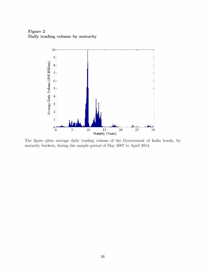
Figure 2Daily trading volume by maturity

The figure plots average daily trading volume of the Government of India bonds, bymaturity buckets, during the sample period of May 2007 to April 2014.

36

Figure 3Time series of bond prices and volume

Panel A: Bond Prices

Panel B: Bond Yields

Panel C: Daily Trading Volume

The figure shows prices, yields and trading volume for the benchmark 10-year maturityGovernment of India bond for the sample period May 21, 2007, to April 20, 2014. PanelA shows the time series of daily closing prices. Panel B shows the time series of dailyclosing yields. Panel C shows the time series of daily trading volume in billions of INR ofbond face value.

37

Figure 4Construction of the inverse slope of the limit order book (ILOBS)

Panel A: Limit Order Book

Price

Quantity

MidpriceBid Ask

Panel B: Construction of ILOBS

Mdist

CQ

0,

,,

,,,

,,,

,,,

,,,

,,

,,

,,

,,

,,

,,

,,,

∆Mdist

∆CQ

ILOBS = ∆Mdist∆CQ

Bid Ask

Panel A depicts the limit order book at a point in time. The horizontal axis shows price,and the vertical axis shows quantity. Each bar represents the total limit order quantity ata particular price. Panel B shows construction of ILOBS associated with the limit orderbook in Panel A. The horizontal axis shows Mdist, the difference between a limit orderprice and the midprice. The vertical axis shows CQ, the cumulative quantity for all limitorders between the midprice and a given limit order price. Bid-side quantities are treatedas negative values. Change, along the fitted line, in CQ is termed as ∆CQ and in Mdistis termed as ∆Mdist.

38

Figure 5Time series of market illiquidity

Market illiquidity is given by the inverse slope of the limit order book (ILOBS) for thebenchmark 10-year maturity Government of India bond and is measured in percentagepoints per billion INR of bond face value. Section 3.2 and Figure 4 give details of theconstruction of ILOBS. Data are sampled at one-minute intervals over the period May21, 2007, to April 20, 2014. The figure shows the time series of daily median ILOBS.

39

Figure 6Time series of volatility

Panel A: Daily volatility of price changes

Panel B: Daily volatility of order flow

Panel C: Ratio of daily volatilities

Data are sampled at one-minute intervals over the period May 21, 2007, to April 20, 2015.Panel A shows the time series of daily volatility of one-minute price changes. Panel Bshows the time series of daily volatility of one-minute order flow. Panel C shows the timeseries of ratio of volatility of order flow to volatility of price changes.

40

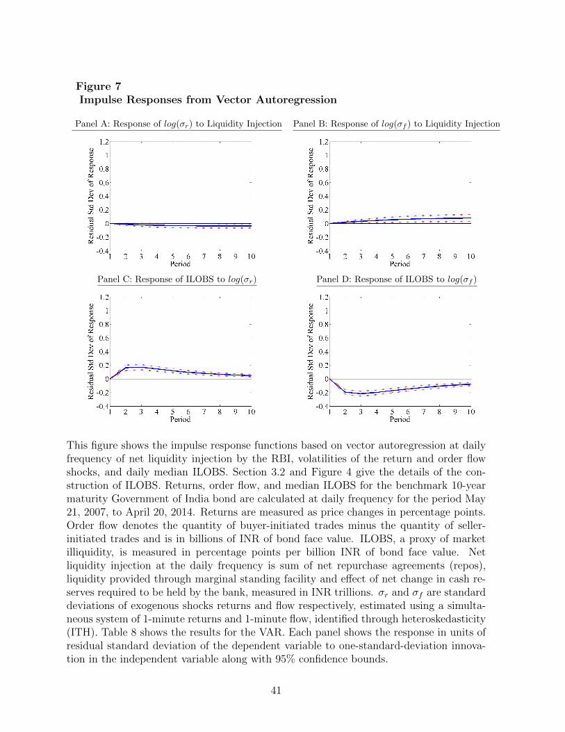
Figure 7Impulse Responses from Vector Autoregression

Panel A: Response of log(σr) to Liquidity Injection Panel B: Response of log(σf ) to Liquidity Injection

Panel C: Response of ILOBS to log(σr) Panel D: Response of ILOBS to log(σf )

This figure shows the impulse response functions based on vector autoregression at dailyfrequency of net liquidity injection by the RBI, volatilities of the return and order flowshocks, and daily median ILOBS. Section 3.2 and Figure 4 give the details of the con-struction of ILOBS. Returns, order flow, and median ILOBS for the benchmark 10-yearmaturity Government of India bond are calculated at daily frequency for the period May21, 2007, to April 20, 2014. Returns are measured as price changes in percentage points.Order flow denotes the quantity of buyer-initiated trades minus the quantity of seller-initiated trades and is in billions of INR of bond face value. ILOBS, a proxy of marketilliquidity, is measured in percentage points per billion INR of bond face value. Netliquidity injection at the daily frequency is sum of net repurchase agreements (repos),liquidity provided through marginal standing facility and effect of net change in cash re-serves required to be held by the bank, measured in INR trillions. σr and σf are standarddeviations of exogenous shocks returns and flow respectively, estimated using a simulta-neous system of 1-minute returns and 1-minute flow, identified through heteroskedasticity(ITH). Table 8 shows the results for the VAR. Each panel shows the response in units ofresidual standard deviation of the dependent variable to one-standard-deviation innova-tion in the independent variable along with 95% confidence bounds.

41

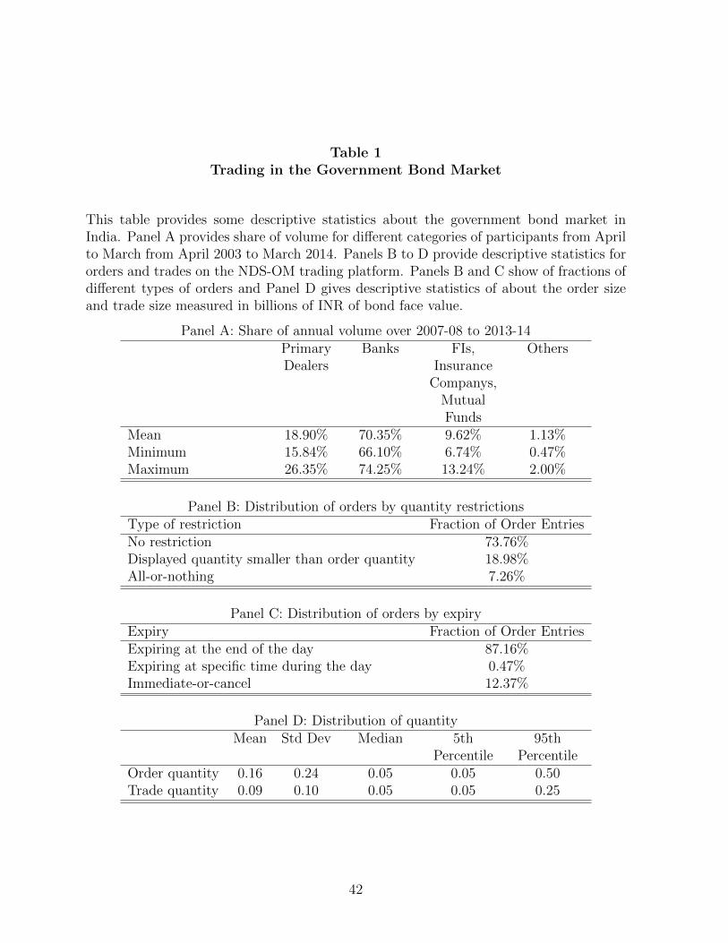
Table 1Trading in the Government Bond Market

This table provides some descriptive statistics about the government bond market inIndia. Panel A provides share of volume for different categories of participants from Aprilto March from April 2003 to March 2014. Panels B to D provide descriptive statistics fororders and trades on the NDS-OM trading platform. Panels B and C show of fractions ofdifferent types of orders and Panel D gives descriptive statistics of about the order sizeand trade size measured in billions of INR of bond face value.

Panel A: Share of annual volume over 2007-08 to 2013-14Primary Banks FIs, OthersDealers Insurance

Companys,MutualFunds

Mean 18.90% 70.35% 9.62% 1.13%Minimum 15.84% 66.10% 6.74% 0.47%Maximum 26.35% 74.25% 13.24% 2.00%

Panel B: Distribution of orders by quantity restrictionsType of restriction Fraction of Order EntriesNo restriction 73.76%Displayed quantity smaller than order quantity 18.98%All-or-nothing 7.26%

Panel C: Distribution of orders by expiryExpiry Fraction of Order EntriesExpiring at the end of the day 87.16%Expiring at specific time during the day 0.47%Immediate-or-cancel 12.37%

Panel D: Distribution of quantityMean Std Dev Median 5th 95th

Percentile PercentileOrder quantity 0.16 0.24 0.05 0.05 0.50Trade quantity 0.09 0.10 0.05 0.05 0.25

42

Table 2Descriptive statistics

This table presents descriptive statistics of price changes, order flow, bid-ask spreads andthe inverse slope of the limit order book (ILOBS) for the benchmark 10-year maturityGovernment of India bond. Price changes and bid-ask spread are in percentage pointsper 100 INR of bond face value. Order flow denotes the quantity of buyer-initiated tradesminus the quantity of seller-initiated trades and is in billions of INR of bond face value.ILOBS, a proxy of market illiquidity, is measured in percentage points per billion INR ofbond face value. Section 3.2 and Figure 4 give the details of the construction of ILOBS.Data are sampled at one-minute intervals over the period May 21, 2007, to April 20, 2014.

Sample Obs Mean Std Dev Median 5th 95thPercentile Percentile

Price Changes 794890 -0.0000 0.0154 0.0000 -0.0150 0.0138Order Flow 855740 0.02 0.27 0.00 -0.20 0.30Bid-Ask Spread 797283 0.04 0.07 0.03 0.01 0.13ILOBS 797790 0.28 0.69 0.14 0.03 0.92

43

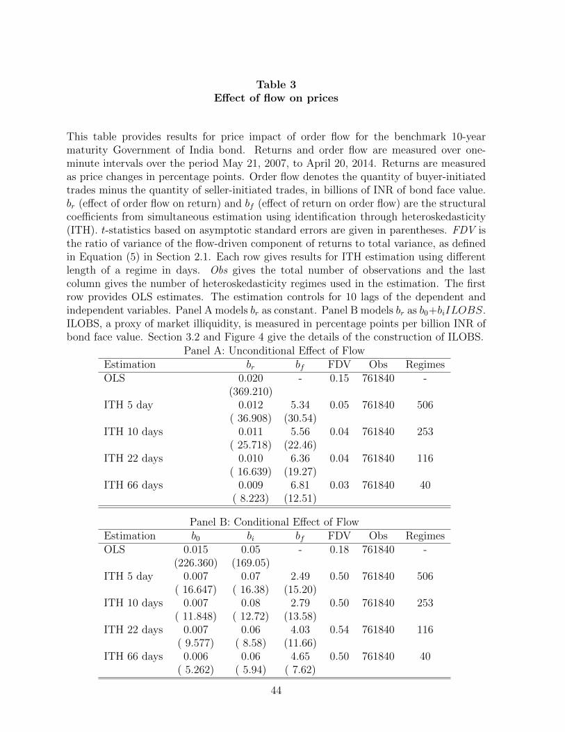
Table 3Effect of flow on prices

This table provides results for price impact of order flow for the benchmark 10-yearmaturity Government of India bond. Returns and order flow are measured over one-minute intervals over the period May 21, 2007, to April 20, 2014. Returns are measuredas price changes in percentage points. Order flow denotes the quantity of buyer-initiatedtrades minus the quantity of seller-initiated trades, in billions of INR of bond face value.br (effect of order flow on return) and bf (effect of return on order flow) are the structuralcoefficients from simultaneous estimation using identification through heteroskedasticity(ITH). t-statistics based on asymptotic standard errors are given in parentheses. FDV isthe ratio of variance of the flow-driven component of returns to total variance, as definedin Equation (5) in Section 2.1. Each row gives results for ITH estimation using differentlength of a regime in days. Obs gives the total number of observations and the lastcolumn gives the number of heteroskedasticity regimes used in the estimation. The firstrow provides OLS estimates. The estimation controls for 10 lags of the dependent andindependent variables. Panel A models br as constant. Panel B models br as b0+biILOBS.ILOBS, a proxy of market illiquidity, is measured in percentage points per billion INR ofbond face value. Section 3.2 and Figure 4 give the details of the construction of ILOBS.

Panel A: Unconditional Effect of FlowEstimation br bf FDV Obs RegimesOLS 0.020 - 0.15 761840 -

(369.210)ITH 5 day 0.012 5.34 0.05 761840 506

( 36.908) (30.54)ITH 10 days 0.011 5.56 0.04 761840 253

( 25.718) (22.46)ITH 22 days 0.010 6.36 0.04 761840 116

( 16.639) (19.27)ITH 66 days 0.009 6.81 0.03 761840 40

( 8.223) (12.51)

Panel B: Conditional Effect of FlowEstimation b0 bi bf FDV Obs RegimesOLS 0.015 0.05 - 0.18 761840 -

(226.360) (169.05)ITH 5 day 0.007 0.07 2.49 0.50 761840 506

( 16.647) ( 16.38) (15.20)ITH 10 days 0.007 0.08 2.79 0.50 761840 253

( 11.848) ( 12.72) (13.58)ITH 22 days 0.007 0.06 4.03 0.54 761840 116

( 9.577) ( 8.58) (11.66)ITH 66 days 0.006 0.06 4.65 0.50 761840 40

( 5.262) ( 5.94) ( 7.62)

44

Table 4Conditional effect of flow on prices: Different specifications

This table presents price impact of order flow conditional on the inverse slope of thelimit order book (ILOBS) estimated using a simultaneous system of return and flow andidentified through heteroskedasticity (ITH). Price changes are in percentage points. Orderflow denotes the quantity of buyer-initiated trades minus the quantity of seller-initiatedtrades and is in billions of INR of bond face value. The table presents a linear specificationwhere return = (b0 + biILOBS)Flow and Flow = bfreturn. Section 3.2 and Figure 4give the details of the construction of ILOBS, a proxy of market illiquidity, measured inpercentage points per billion INR of bond face value. Returns, order flow, and ILOBS forthe benchmark 10-year maturity Government of India bond are calculated over one-minuteor five-minute intervals over the period May 21, 2007, to April 20, 2014. t-statistics basedon asymptotic standard errors are in parentheses. FDV is the ratio of variance of theflow-driven component of returns to total variance, as defined in Equation (5) in Section2.1. ITH estimation is done using 10-day regimes. Panel A presents results for one-minute and five-minute intervals controlling for different number of lags of the dependentand independent variables. Panel B shows results conditioning on different versions ofILOBS or bid-ask spread using returns and flow over one-minute intervals controllingfor 10 lags of the dependent and independent variables. ILOBS-Narrow is based on thebest bid and the best ask quotes. ILOBS-Asymmetric is ILOBS for ask side for positivenet flow and ILOBS for bid side for negative net flow. ILOBS-wt1 and ILOBS-wt2 areinverse of the weighted slope of the limit order book. Weights are, respectively, inverseof the absolute distance from the midprice and inverse of the squared distance from themidprice. Bid-ask spread is the difference, in percentage points, between best ask andbest bid quotes.

Panel A: Different Intervals, Different LagsEstimation b0 b1 bf FDV1-Minute Interval, 5 lags 0.007 0.07 2.85 0.56

(11.749) (12.73) (13.83)1-Minute Interval, 10 lags 0.007 0.08 2.79 0.50

(11.848) (12.72) (13.58)1-Minute Interval, 15 lags 0.007 0.08 2.73 0.51

(11.893) (12.70) (13.32)5-Minute Interval, 1 lag 0.007 0.08 5.68 0.49

(13.285) (13.71) (17.04)5-Minute Interval, 3 lags 0.007 0.08 5.41 0.46

(13.030) (14.70) (16.95)5-Minute Interval, 5 lags 0.006 0.09 5.17 0.50

(12.682) (14.87) (16.71)

45

Panel B: Conditioning on Different Versions of ILOBSEstimation b0 b1 bf FDVILOBS 0.007 0.08 2.79 0.50

( 11.848) ( 12.72) (13.58)ILOBS-Narrow 0.0010 0.17 0.36 0.49

( 2.4139) ( 43.11) ( 4.86)ILOBS-Asymmetric 0.0119 0.04 4.29 0.51

( 26.7810) ( 6.84) (16.03)ILOBS-wt1 0.012 0.08 3.95 0.47

( 26.652) ( 9.02) (15.25)ILOBS-wt2 0.0121 0.13 3.85 0.49

( 26.5770) ( 10.36) (15.16)Bid-Ask Spread -0.0036 0.88 0.67 0.44

( -5.7659) ( 35.07) ( 6.44)

46

Table 5Impulse response

This table provides estimates of instantaneous and long-run impact of one-standard-deviation shock to the innovations in order flow and returns for the benchmark 10-yearmaturity Government of India bond using identification through heteroskedasticity (ITH)corresponding to the results presented in Table 3, Panel B for 10-day volatility regimes.“Shock to Flow” columns present impact of a shock to the innovations in order flow.“Shock to Returns” columns present impact of a shock to the innovations in returns. Ii,j,0and Ii,j,∞, respectively, capture instantaneous and long-run responses of variable j to ashock to variable i. i and j can be r for returns or f for order flow. Returns and orderflow are measured over one-minute intervals over the period May 21, 2007, to April 20,2014. Returns are measured as price changes in percentage points. Order flow denotesthe quantity of buyer-initiated trades minus the quantity of seller-initiated trades and isin billions of INR of bond face value. ILOBS, a proxy of market illiquidity, is measured inpercentage points per billion INR of bond face value. Different rows in each panel reportthe responses conditional on ILOBS being at its 5th, 50th, and 95th percentiles.

Shock to Flow Shock to ReturnsILOBS If,r,0 If,r,∞ If,f,0 If,f,∞ Ir,r,0 Ir,r,∞ Ir,f,0 Ir,f,∞5th %ile 0.19 0.24 1.03 1.78 1.03 1.01 0.14 0.3050th %ile 0.37 0.52 1.05 1.82 1.05 1.05 0.15 0.3195th %ile 1.93 2.82 1.27 2.13 1.27 1.45 0.18 0.37

47

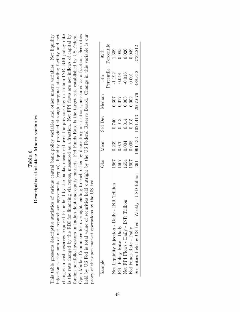
Table

6D

esc

ripti

ve

stati

stic

s:M

acr

ovari

able

s

This

table

pre

sents

des

crip

tive

stat

isti

csof

vari

ous

centr

alban

kp

olic

yva

riab

les

and

other

mac

rova

riab

les.

Net

liquid

ity

inje

ctio

nis

the

sum

ofnet

repurc

has

eag

reem

ents

(rep

os),

liquid

ity

pro

vid

edth

rough

mar

ginal

stan

din

gfa

cility

and

net

chan

ges

inca

shre

serv

esre

quir

edto

be

hel

dby

the

ban

ks,

mea

sure

dov

erth

epre

vio

us

day

intr

illion

INR

.R

BI

pol

icy

rate

isth

era

tech

arge

dby

the

RB

Ifo

rfinan

cing

via

rep

os,

mea

sure

das

afr

acti

on.

Net

FP

Iflow

sar

enet

inflow

sof

capit

alby

fore

ign

por

tfol

ioin

vest

ors

inIn

dia

ndeb

tan

deq

uit

ym

arke

ts.

Fed

Funds

Rat

eis

the

targ

etra

tees

tablish

edby

US

Fed

eral

Op

enM

arke

tC

omm

itte

efo

rov

ernig

ht

lendin

gto

each

other

by

dep

osit

ory

inst

ituti

ons,

mea

sure

das

afr

acti

on.

Sec

uri

ties

hel

dby

US

Fed

isto

tal

valu

eof

secu

riti

eshel

dou

trig

ht

by

the

US

Fed

eral

Res

erve

Boa

rd.

Chan

gein

this

vari

able

isou

rpro

xy

ofth

eop

enm

arke

top

erat

ions

by

the

US

Fed

.

Sam

ple

Obs

Mea

nStd

Dev

Med

ian

5th

95th

Per

centi

leP

erce

nti

leN

etL

iquid

ity

Inje

ctio

n-

Dai

ly-

INR

Tri

llio

n16

670.

239

0.74

00.

307

-1.1

921.

309

RB

IP

olic

yR

ate

-D

aily

1667

0.07

00.

013

0.07

70.

048

0.08

5N

etF

PI

Flo

ws

-D

aily

-IN

RT

rillio

n16

540.

004

0.01

40.

003

-0.0

160.

026

Fed

Funds

Rat

e-

Dai

ly16

070.

008

0.01

50.

002

0.00

10.

049

Sec

uri

ties

Hel

dby

US

Fed

-W

eekly

-U

SD

Billion

361

1991

.133

1021

.413

2067

.676

488.

312

3732

.212

48

Table 7Conditioning on central bank policies

This table presents price impact of order flow conditional on the inverse slope of the limitorder book (ILOBS) and central bank policy, estimated using a simultaneous system ofreturn and flow and identified through heteroskedasticity (ITH). Returns are measuredas price changes in percentage points. Order flow denotes the quantity of buyer-initiatedtrades minus the quantity of seller-initiated trades and is in billions of INR of bondface value. Section 3.2 and Figure 4 give the details of the construction of ILOBS, aproxy of market illiquidity, measured in percentage points per billion INR of bond facevalue. Returns, order flow, and ILOBS for the benchmark 10-year maturity Governmentof India bond are calculated over the period May 21, 2007, to April 20, 2014. Panels A,C and D present specifications where Flow = bfreturn and return = brFlow. Panel Ahas br = b0 + biILOBS + bp−lqPolicy − Lq + bp−rtPolicy − Rate. Policy − Lq is dailynet liquidity injection by RBI. Policy − Rate is the RBI policy rate. Panel B has br =b0+biILOBS+bp−lqinPolicy−Injection+bp−lqwdPolicy−Withdrawal. Policy−Injectionis equal to daily net liquidity injection when the net injection is positive and zero otherwise.Policy −Withdrawal is equal the daily net liquidity injection when the net injection isnegative and zero otherwise. Net liquidity injection is the sum, over the previous day, ofnet repurchase agreements (repos), liquidity provided through marginal standing facilityand changes to cash reserves required to be held by banks and is measured in trillionINR. RBI policy rate is the repo rate lagged by one day and is measured as a fraction.t-statistics based on asymptotic standard errors are in parentheses. FDV is the ratio ofvariance of the flow-driven component of returns to total variance, as defined in Equation(5) in Section 2.1. In Panels A, B and C, the estimation uses returns and flow overone-minute intervals, controls for 10 lags of the dependent and independent variables anduses ITH 10-day regimes. In Panel D, the estimation uses returns and flow over one-dayintervals, controls for 5 lags of the dependent and independent variables and uses ITH10-day regimes.

Panel A: Conditioning on Policy VariablesPolicy Variable b0 bi bp−lq bp−rt bf FDVNet Liquidity Injectionand RBI Policy Rate -0.006 0.07 -0.0054 0.22 2.72 0.52

(-1.850) ( 10.82) ( -7.4238) ( 5.15) (14.20)Net Liquidity Injection 0.010 0.06 -0.0039 2.77 0.49

( 14.135) ( 10.15) ( -6.3288) (13.97)RBI Policy Rate -0.000 0.08 0.09 2.77 0.50

( -0.107) ( 12.95) ( 2.42) (13.57)

49

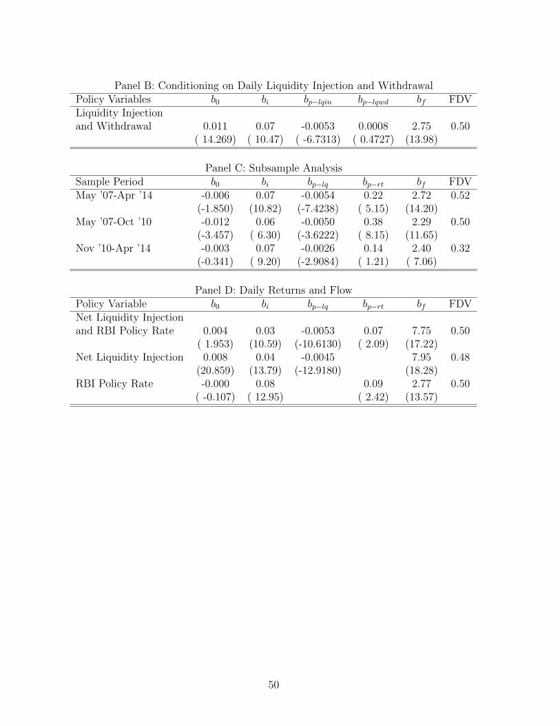
Panel B: Conditioning on Daily Liquidity Injection and WithdrawalPolicy Variables b0 bi bp−lqin bp−lqwd bf FDVLiquidity Injectionand Withdrawal 0.011 0.07 -0.0053 0.0008 2.75 0.50

( 14.269) ( 10.47) ( -6.7313) ( 0.4727) (13.98)

Panel C: Subsample AnalysisSample Period b0 bi bp−lq bp−rt bf FDVMay ’07-Apr ’14 -0.006 0.07 -0.0054 0.22 2.72 0.52

(-1.850) (10.82) (-7.4238) ( 5.15) (14.20)May ’07-Oct ’10 -0.012 0.06 -0.0050 0.38 2.29 0.50

(-3.457) ( 6.30) (-3.6222) ( 8.15) (11.65)Nov ’10-Apr ’14 -0.003 0.07 -0.0026 0.14 2.40 0.32

(-0.341) ( 9.20) (-2.9084) ( 1.21) ( 7.06)

Panel D: Daily Returns and FlowPolicy Variable b0 bi bp−lq bp−rt bf FDVNet Liquidity Injectionand RBI Policy Rate 0.004 0.03 -0.0053 0.07 7.75 0.50

( 1.953) (10.59) (-10.6130) ( 2.09) (17.22)Net Liquidity Injection 0.008 0.04 -0.0045 7.95 0.48

(20.859) (13.79) (-12.9180) (18.28)RBI Policy Rate -0.000 0.08 0.09 2.77 0.50

( -0.107) ( 12.95) ( 2.42) (13.57)

50

Table 8Vector Autoregression

This table presents results of vector autoregression at daily frequency of net liquidityinjection by the RBI, volatilities of the return and order flow shocks, and daily medianILOBS. Net liquidity injection is the sum of net repurchase agreements (repos), liquidityprovided through marginal standing facility and net change in cash reserves required tobe held by the banks, measured in trillion INR. σr and σf are daily standard deviationsof exogenous shocks to one-minute returns and one-minute flow respectively, estimatedusing a simultaneous system of return and flow, identified through heteroskedasticity(ITH). Returns are measured as price changes in percentage points. Order flow denotesthe quantity of buyer-initiated trades minus the quantity of seller-initiated trades and isin billions of INR of bond face value. Section 3.2 and Figure 4 give the details of theconstruction of ILOBS, a proxy of illiquidity, measured in percentage points per billionINR of bond face value. Returns, order flow, and median ILOBS are for the benchmark10-year maturity Government of India bond for the period May 21, 2007, to April 20,2014. The variables in the VAR are scaled by their own standard deviation. Panel Apresents coefficients and t-stats in parentheses. Panel B shows the correlations of theresiduals from the VAR.

Panel A: Coefficient EstimatesLiquidity Injection log(σr) log(σf ) ILOBS

Liquidity Injection (-1) 0.955 -0.035 0.035 0.018(132.259) (-1.825) (2.380) (0.816)

log(σr(−1)) -0.015 0.659 -0.078 0.190(-2.036) (33.669) (-5.248) (8.341)

log(σf (−1)) 0.009 -0.033 0.831 -0.299(1.169) (-1.538) (51.454) (-12.039)

ILOBS(-1) -0.009 0.037 0.018 0.260(-1.157) (1.786) (1.127) (10.686)

Adj. R-squared 0.923 0.452 0.686 0.260

Panel B: Residual CorrelationsLiquidity Injection log(σr) log(σf ) ILOBS

Liquidity Injection 1.000 0.063 0.054 0.005log(σr(−1)) 0.063 1.000 0.370 0.113log(σf (−1)) 0.054 0.370 1.000 -0.160ILOBS 0.005 0.113 -0.160 1.000

51

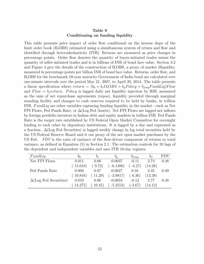
Table 9Conditioning on funding liquidity

This table presents price impact of order flow conditional on the inverse slope of thelimit order book (ILOBS) estimated using a simultaneous system of return and flow andidentified through heteroskedasticity (ITH). Returns are measured as price changes inpercentage points. Order flow denotes the quantity of buyer-initiated trades minus thequantity of seller-initiated trades and is in billions of INR of bond face value. Section 3.2and Figure 4 give the details of the construction of ILOBS, a proxy of market illiquidity,measured in percentage points per billion INR of bond face value. Returns, order flow, andILOBS for the benchmark 10-year maturity Government of India bond are calculated overone-minute intervals over the period May 21, 2007, to April 20, 2014. The table presentsa linear specification where return = (b0 + biILOBS + bpPolicy + bfnlqFundLiq)Flowand Flow = bfreturn. Policy is lagged daily net liquidity injection by RBI, measuredas the sum of net repurchase agreements (repos), liquidity provided through marginalstanding facility and changes to cash reserves required to be held by banks, in trillionINR. FundLiq are other variables capturing funding liquidity in the market - such as NetFPI Flows, Fed Funds Rate, or ∆(Log Fed Assets). Net FPI Flows are lagged net inflowsby foreign portfolio investors in Indian debt and equity markets in trillion INR. Fed FundsRate is the target rate established by US Federal Open Market Committee for overnightlending to each other by depository institutions. It is lagged by a day and expressed asa fraction. ∆(Log Fed Securities) is lagged weekly change in log total securities held bythe US Federal Reserve Board and it our proxy of the net open market purchases by theUS Fed. FDV is the ratio of variance of the flow-driven component of returns to totalvariance, as defined in Equation (5) in Section 2.1. The estimation controls for 10 lags ofthe dependent and independent variables and uses ITH 10-day regimes.

FundLiq b0 bi bp bfnlq bf FDVNet FPI Flows 0.011 0.06 -0.0037 -0.11 2.74 0.48

( 15.018) ( 9.72) ( -6.1380) ( -4.27) (14.28)Fed Funds Rate 0.008 0.07 -0.0027 0.16 2.45 0.49

( 10.816) ( 11.29) ( -3.9817) ( 6.36) (13.38)∆(Log Fed Securities) 0.010 0.06 -0.0034 -0.12 2.77 0.48

( 14.275) ( 10.45) ( -5.2553) (-3.67) (14.12)

52