Central Bank Macro Modeling

Christopher A. SimsPrinceton Universitysims@princeton.edu

March 8, 2018

c©2018 by Christopher A. Sims. c©2018. This document is licensed under the Creative CommonsAttribution-NonCommercial-ShareAlike 3.0 Unported License.http://creativecommons.org/licenses/by-nc-sa/3.0/

Outline

• Methods, model types

• Monetary policy responses

• Financial shock responses

• Comparison to BPSS

• Absence of credit expansion → crisis

1

What’s missing

• Fiscal-monetary interaction

• “Heterogeneity”

• How to model financial frictions: intermediation vs. net worth vs.liquidity

• Inattention and bounded rationality

2

Methods, model types

• Most of the models are variants on New Keynesian DSGE’s.

• FRBUS and JEM are major exceptions.

• Most calibrate some parameters, estimate some others with “Bayesianmethods”.

3

Should we be worried about sticking with NK DSGE’s?

• They didn’t start out with financial sectors or financial frictions, but wecan add them, and are doing so.

• They ignore or assume away intertemporal aspects of fiscal policy, butwe can add them, though we are not doing so.

• They imply price level indeterminacy at the ZLB, which seriously limitstheir usefulness (a euphemism) for policy analysis in low interest rateenvironments.

• They center on the NK Phillips curve, a story no one believes except asa kind of “metaphor” to explain why nominal things have real effects.

4

• Still, as a starting point, they are the best we have.

• We should recognize that they arose as a way to tell more elaboratestories that remain consistent with SVAR’s. We should not lose sight ofthat SVAR foundation as we elaborate and revise the DSGE framework.

5

FRBUS and JEM

• This approach has the claimed advantage that it allows equations andsectors to be added, subtracted, or respecified without changing the restof the model.

• This approach allows bigger models at a given computational constraintlevel.

• But in the end it is not much different from regressing quantity and priceand calling that “demand” and regressing price on quantity and callingthat “supply”.

6

Can FRBUS and JEM be useful?

• It is possible that FRBUS and JEM have enough recursive structure thatthey are close to restricted triangular VAR’s, which would justify usingthe equation-by-equation OLS that they are largely based on.

• But I’ve seen no attempt to check this, i.e. to see how much impliedsimultaneity there is in the system and whether it can be isolated.

• This is not to say the models are useless. They can be a framework toenforce consistency among expert opinios, as can a spreadsheet. Theyjust cannot be taken seriously as probability models of the data.

7

Calibration

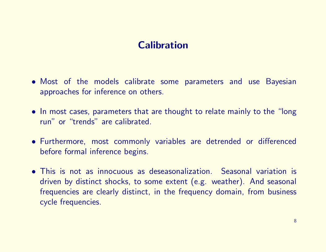
• Most of the models calibrate some parameters and use Bayesianapproaches for inference on others.

• In most cases, parameters that are thought to relate mainly to the “longrun” or “trends” are calibrated.

• Furthermore, most commonly variables are detrended or differencedbefore formal inference begins.

• This is not as innocuous as deseasonalization. Seasonal variation isdriven by distinct shocks, to some extent (e.g. weather). And seasonalfrequencies are clearly distinct, in the frequency domain, from businesscycle frequencies.

8

• We know that separating trend and business cycle frequencies is not easy(Granger’s “typical spectral shape”).

• Bayesian model comparison can be seriously distorted if uncertaintyarising from detrending is not treated explicitly.

9

Estimation

• There are two sources of appeal for Bayesian approaches:

• They allow, via the prior, proceeding with models that have some weaklyidentified parameters, as large models generally do.

• They provide an internally consistent way to model parameter uncertaintyand thereby potentially a way to provide realistic measures of uncertaintyabout model predictions.

10

The COMPASS priors and posteriors (an example)

• There are many parameters (about 50), all given independent priors.This in itself is hazardous, likely implying some unintended dogmaticbeliefs.

• Many of the prior standard deviations seem to me unrealistically tight.For a decision-making model, we should use tighter priors than in ascientific paper where we are hoping to persuade an audience of diverseviews, but these seem tight even by that standard. The line betweencalibration and estimation is thin here.

• Some prior means for variances have been set by looking at the data.This seems hard to justify.

11

• For many parameters, prior standard deviations and means are close toposteriors. These parameters are probably weakly identified. Since priorsfor them are very important, they deserve special attention.

• Exploration of variants on the prior would be a good idea.

• The Bayesian approach is allowing use of a large model with weaklyidentified parameters, but it is probably not providing realistic assessmentsof posterior uncertainty.

12

Responses to monetary policy shocks

• The models imply quite similar patterns of response to monetary policytightening.

• With full rational expectations, the responses are unrealistically front-loaded, implying strong, within-quarter, effects on GDP and prices.

• This is unsurprising, and not just a result of everyone copying Smets andWouters. SVAR’s have shown us that these patterns are robust acrosstime, countries, and identificaions strategies.

13

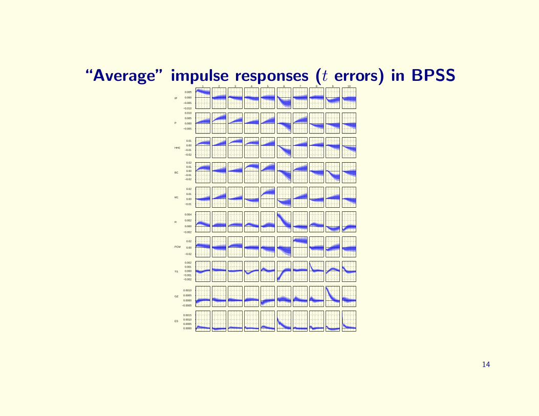
“Average” impulse responses (t errors) in BPSSIP

−0.010

−0.005

0.000

0.005

1 2 3 4 5 6 7 8 9 10

P

−0.005

0.000

0.005

0.010

HHC

−0.02

−0.01

0.00

0.01

BC

−0.02

−0.01

0.00

0.01

0.02

M1

−0.01

0.00

0.01

0.02

R

−0.002

0.000

0.002

0.004

PCM

−0.02

0.00

0.02

TS

−0.002

−0.001

0.000

0.001

0.002

GZ

−0.0005

0.0000

0.0005

0.0010

ES

0.0000

0.0005

0.0010

0.0015

14

Financial shocks

• In some cases, these responses are close to scalings of the monetarypolicy shock responses.

• In the NY Fed model at least, the effects of financial shocks are morepersistent than the effects of a monetary policy shock.

• This is not there in the BPSS VAR, even though in the BPSS VAR thefinancial shocks play the same role in making forecasts during the greatrecession more pessimistic and realistic.

• None of the models, including BPSS, show low interest rates or expansionof credit aggregates creating a crisis. This is not a defect.

15

Fiscal/Monetary interaction

• These models, with their attention to bringing in financial frictions, maybe fighting the last war.

• Unbacked fiscal expansion produces inflation, and may do so in the faceof resistance from the central bank in the form of interest rate increases.

• If markets perceive the fiscal expansion as unbacked, interest rateincreases exacerbate, rather than end, inflation.

• We do not see much of this historically in rich country data — just aswe did not see many major financial crashes historically in postwar richcountry data.

16

• But we should have our models ready to analyze this if it occurs.

• Models that begin by assuming zero government debt and/or zerodeficits and/or passive fiscal policy with lump sum taxes, and therebyjustify ignoring wealth effects of government debt, cannot help us here.

• Leeper, Traum and Walker have shown us that a model that includesdynamic fiscal policy and recognizes the difficulty of separating causalinfluences of monetary and fiscal policy in the historical data, is possible.

17

Heterogeneity

• The HANK model demonstrates that recognizing a wider array of agenttypes in NK models, with a more realistic treatment of liquidity, canchange our conclusions about how monetary policy works.

• One implication of HANK, that its authors emphasizie, is that Ricardianequivalence is far from holding.

• Since monetary policy induced interest rate changes require fiscalresponses under passive fiscal policy, the effects of monetary policydepend strongly on the fiscal response. Another reason to pay moreattention to the dynamics of fiscal policy.

18

Heterogeneity

• But the non-neutrality of fiscal policy and the uncertainties this impliesfor the effects of monetary policy are the tip of the iceberg.

• As we disaggregate, the number of interactions across markets and agenttypes grows explosively.

• We don’t have strong evidence about many of these connections, andit may be tempting to make simplifying assumptions to bound modelcomplexity.

• This runs the risk of models that tell richer stories, while becoming worse,not better, at tracking the major aggregates.

19

• As we proceed into the thickets of heterogeneous-agent modeling, it isimportant to maintain the requirement that the models should not doworse than SVAR’s at tracking the main aggregates.

20

Inattention and bounded rationality

• Mackowiak and Wiederholt have shown that inattention can beincorporated into a DSGE and that this is at least a partial substitute forother sources of “stickiness”.

• Their model also, like HANK, implies that welfare analysis of monetarypolicy could be sensitive to the presence of this complication.

• But their setup is special. Models where markets have agents on bothsides subject to RI constraints are much harder.

• But RI is likely to be pervasive. Recognizing that should make us realizethat sluggish adjustment will be pervasive, and that it is dangerous tointerpret it as created by “adjustment costs”.

21

Machine learning?

• Importing numerical methods from the machine learning literature maylet us handle bigger, more non-linear models.

• This opens possibilities, but also, as mentioned earlier, pitfalls. Morecomplicated models that fit less well or mask uncertainty with calibratedparameters or unrealistically tight priors are not an improvement.

• ¡Aside on the difference between economic modeling and imagerecognition¿

22

Conclusion

• There’s lots of important work to do. My own priorities:

– Dynamic analysis of fiscal policy, with wealth effects, and therebycreating the possibility of modeling fiscal dominance.

– Expanded and more sophisticated weakly identified models in the spiritof SVAR’s, to provide a well-fitting benchmark to discipline DSGE-stylemodels.

23