Research Division Federal Reserve Bank of St. Louis Working Paper Series

Central Bank Intervention with Limited Arbitrage

Christopher J. Neely and

Paul A. Weller

Working Paper 2006-033B http://research.stlouisfed.org/wp/2006/2006-033.pdf

May 2006 Revised February 2007

FEDERAL RESERVE BANK OF ST. LOUIS Research Division

P.O. Box 442 St. Louis, MO 63166

______________________________________________________________________________________

The views expressed are those of the individual authors and do not necessarily reflect official positions of the Federal Reserve Bank of St. Louis, the Federal Reserve System, or the Board of Governors.

Federal Reserve Bank of St. Louis Working Papers are preliminary materials circulated to stimulate discussion and critical comment. References in publications to Federal Reserve Bank of St. Louis Working Papers (other than an acknowledgment that the writer has had access to unpublished material) should be cleared with the author or authors.

Central bank intervention with limited arbitrage

Christopher J. Neely1

Paul A. Weller2

February 3, 2007

Abstract: Shleifer and Vishny (1997) pointed out some of the practical and theoretical problems associated with assuming that rational risk-arbitrage would quickly drive asset prices back to long-run equilibrium. In particular, they showed that the possibility that asset price disequilibrium would worsen, before being corrected, tends to limit rational speculators. Uniquely, Shleifer and Vishny (1997) showed that “performance-based asset management” would tend to reduce risk-arbitrage when it is needed most, when asset prices are furthest from equilibrium. We analyze a generalized Shleifer and Vishny (1997) model for central bank intervention. We show that increasing availability of arbitrage capital has a pronounced effect on the dynamic intervention strategy of the central bank. Intervention is reduced during periods of moderate misalignment and amplified at times of extreme misalignment. This pattern is consistent with empirical observation.

Keywords: Intervention, foreign exchange, limits to arbitrage, arbitrage, noise trader

JEL Codes: F3, F31, E58

1 Christopher J. Neely Research Officer Research Department Federal Reserve Bank of St. Louis neely@stls.frb.org (314) 444-8568 (f) (314) 444-8731 (o)

2 Paul A. Weller Professor Department of Finance University of Iowa paul-weller@uiowa.edu (319) 335-1017 (o)

The views expressed are those of the authors and not necessarily those of the Federal Reserve

Bank of St. Louis or the Federal Reserve System.

The behavior of foreign exchange rates has puzzled economists since the breakdown of

Bretton Woods in 1973. First, exchange rates do not covary with interest rate differentials in any

explicable way in the short- and medium-term (Hodrick (1987), Engel (1996) and Meredith and

Chinn (1998)). Second, a large literature has documented successful trend-following technical

trading rules in foreign exchange markets (e.g., Sweeney (1986), Neely, Weller and Dittmar

(1997)). Third, foreign exchange rates are only weakly connected to fundamentals over long

horizons. (Meese and Rogoff (1983), Kilian (1999), Engel (2000), Mark and Sul (2001) and

Rapach and Wohar (2002), Neely and Sarno (2002). One might interpret the evidence to

indicate that exchange rates are connected to fundamentals in the long-run and/or under extreme

conditions, but that exchange rates can deviate substantially from their fundamental values for

significant periods. This misalignment of exchange rates presents a puzzle: Why is there

apparently insufficient risk-arbitrage to keep foreign exchange rates in line with fundamentals?

Some researchers have sought to create general equilibrium models in which exchange

rates seem to be disconnected from fundamentals, e.g. Duarte and Stockman (2002). Such

models are not yet wholly convincing; they cannot explain the behavior of risk premia or

variation in exchange rates. Models containing features such as noise trading and/or limits to

arbitrage are also widely used (e.g., Devereux and Engel (2002), Duarte and Stockman (2001)).

Other researchers have turned to bounded rationality or behaviorally based departures

from rationality to generate the apparently volatile expectations of exchange rates. For example,

Frankel (1996) argues that exchange rates are detached from fundamentals by swings in

expectations about future values of the exchange rate. Four pieces of evidence suggest that

overly volatile expectations are to blame for such behavior: 1) Survey measures of exchange rate

expectations are very poor forecasts and are often not internally consistent (Frankel and Froot,

1

1987, Sarno and Taylor 2001); 2) the failure of uncovered interest parity (UIP) seems to hinge

on irrational expectations (Engel, 1996); 3) Trend-following trading rules make risk-adjusted

excess returns (Neely, 1997; Neely, Weller, and Dittmar, 1997); 4) Switching from a fixed to a

floating exchange rate changes the volatility of real exchange rates and the ability of UIP to

explain exchange rate changes (Mussa, 1986).

The volatile expectations of an apparently economically significant group of agents have

created misalignments—predictable long-term returns—that are potentially exploitable.

Monetary authorities have invested in foreign exchange in anticipation of such long-run

reversion to fundamentals. Neely (2005) summarizes evidence that major central banks, those of

the United States, Germany, Japan, Switzerland and Australia, have made excess returns–returns

on a zero investment strategy–on their foreign exchange intervention by “buying-low and

selling-high” (Leahy (1995), Neely (1998), Sweeney (1997), Sjöö and Sweeney (2001)). These

predictable long-term returns are associated with deviations from PPP fundamentals.

There are doubtless private agents with realistic expectations who similarly profit from

fundamental-based investments. But these agents—coupled with central banks—do not seem to

have enough market power to prevent persistent and large departures from fundamentals. Why

is there not more private risk arbitrage?

A growing literature argues that various limits to arbitrage reduce the speed with which

rational speculators can push rates back to fundamentals. Noise trading in the presence of

fundamental risk makes arbitrage risky (De Long et al., 1990). Shleifer and Vishny (1997)

(hereafter SV) explored how traders are constrained by risk and principal-agent problems. In

particular, SV argue that arbitrage is limited in asset markets because the marginal investor in

asset markets is a highly specialized agent who loses resources precisely when asset prices

2

diverge far from fundamental values. Specifically, the SV argument depends on the existence of

performance-based arbitrage (PBA). PBA means that the capital available to arbitrageurs

depends on the recent returns to their portfolios. When foreign exchange rates diverge further

from fundamentals, fundamental-based traders (FBTs) lose money. As the divergence worsens,

so does the performance of FBTs, both directly because of their losses and because principals

provide less capital. The loss of capital means that risk-arbitrage investment in anticipation of a

return to fundamentals fails precisely as divergence from fundamentals worsens, leading to

greater divergence.

Thus, although risky arbitrage will certainly exert a force in the long run to correct

deviations from fundamentals, this force is attenuated in the short run. The weakness of risky

arbitrage will lead to potentially significant misallocation of resources as trade and investment

decisions are made on the basis of distorted price signals.

The limits-to-arbitrage argument is especially relevant for foreign exchange, where there

is a great deal of uncertainty about fundamentals and very long horizons for mean reversion.

While such uncertainty surely exacerbates the PBA that stems from principal-agent problems,

monetary authorities are likely to be less affected by the forces that drive PBA. Central banks

have proved that they are willing to take long-term positions on reversion to fundamentals and

they have a vested interest in reducing misalignments with sterilized intervention.1

This paper seeks to answer the following: How does the presence of capital dedicated to

risk arbitrage influence the intervention strategy of a central bank facing fundamental

uncertainty? To this end, we extend the SV model to include a central bank and fundamental

uncertainty in addition to rational arbitrageurs.

1 Krugman and Miller (1993) make a related argument in showing how central bank intervention can stabilize exchange rates if speculators are subject to rules that require them to limit their maximum “drawdown”.

3

Much of the theoretical debate about the impact of intervention has focused on

informational issues. Our analysis complements the existing literature by looking at the strategic

interaction between arbitrageurs and the central bank in an environment in which the bank has a

longer time horizon and is not subject to the same short-term pressures that limit the actions of

professional arbitrageurs.

We examine optimal intervention policy in a model which extends that of SV by

introducing a central bank who plays the role of a Stackelberg leader in an intervention game.

The bank’s objective function values both trading profitability and stabilization of the exchange

rate around its fundamental value. We are particularly interested in characteristics of intervention

strategy in the situation where the effects of arbitrage are weakened. The presence of arbitrageurs

in the market makes a difference to the optimal intervention policy. If the central bank intervenes

aggressively during periods of moderate misalignment, but when there is a possibility that the

misalignment will get worse, it risks weakening the synergistic effect of risk arbitrage. This

happens because the intervention increases the short run losses of arbitrageurs and reduces the

funds they have available to bear against misalignment in the future. Using the same logic, we

identify a “high-powered” intervention effect when deviations from fundamentals are unusually

large. We show that the combination of these two effects has a substantial impact on the dynamic

intervention strategy of the central bank.

2. The Limits to Arbitrage Literature

The limits-to-arbitrage concept has significantly influenced thinking on asset pricing.

Indeed, Barberis and Thaler (2002) define limits to arbitrage as one of the building blocks of

behavioral finance.

4

While SV made a generic argument about the limits to arbitrage in general asset markets

others have used the concept to explain or rationalize behavior in specific contexts. Collins,

Gong and Hribar (2003) argue that limits to arbitrage prevent institutional investors from

exploiting the apparently abnormal returns enjoyed by firms with low institutional ownership.

Brunnermeier and Nagel (2004) find that rational investors (hedge funds) captured much of the

upswing in technology stocks but were able to reduce their exposure before the crash. They

argue that limits to arbitrage might contribute to the preference for rational investors to ride

bubbles and destabilize prices. Brav, Heaton and Rosenberg (2004) criticize both rational and

behavioral finance for a lack of testable predictions. But they argue that ex post explanations

support the limits of arbitrage arguments on which behavioral finance relies. Gabaix,

Krishnamurthy, and Vigneron (2005) examine the mortgage-backed securities (MBS) market

through the lens of limits to arbitrage theory. They find that the pricing of homeowner

prepayment risk is consistent with the specialized arbitrageur hypothesis. Massa, Peyer, and

Tong (2005) examine the equity performance and investment in the 2 years after a firm is added

to an index. They find behavior that supports a limits to arbitrage theory. McMillan (2005)

compares nonlinear dynamics in asset returns from European to Asian markets, concluding that

limits to arbitrage are greater in Asian markets. Stein (2005) uses the limits-to-arbitrage concept

to explain the existence of open-end funds and the coexistence of large mispricings with rational,

competitive arbitrageurs. Greenwood (2005) develops testable predictions from a limits-to-

arbitrage framework with multiple risky assets; Nikkei 225 data support these predictions. Jiang,

Lee, and Zhang (2005) examine the relationship between uncertainty in estimates of firm value

and equilibrium returns. Their findings are consistent with models that incorporate limits to

rational arbitrage.

5

Not all papers find support for limits-to-arbitrage models. Gallagher and Taylor (2001),

for example, evaluate a risky arbitrage hypothesis versus a limits-to-arbitrage hypothesis in U.S.

equity markets. They find that the speed of mean reversion favors the risky arbitrage hypothesis.

3. The Model

We extend the model developed by Shleifer and Vishny (1997) in the following ways.

We apply the model specifically to the foreign exchange market, introduce a central bank in

addition to arbitrageurs and also permit uncertainty about fundamentals. For concreteness we

assume that the problem involves U.S. based arbitrageurs, noise traders, a foreign central bank,

and that the foreign currency is the euro. There are three time periods. The expected fundamental

value of the euro (the exchange rate measured as the dollar price of the euro) at time t is . It

becomes known either at time 2 or at time 3. It can take on two values, and with equal

probability. Its expected value is

tV

HV LV

V The exchange rate at time t, t =1, 2 is tp . In each of the first

two periods noise traders experience a pessimism shock. At time 1, the first period shock 1S

known to arbitrageurs and to the central bank, but the second period shock, is not. The

shocks affect noise trader demand for the euro at time t, . (Note that the cumulative second

period shock is the sum of the first period shock and the increment, , to the first shock.)

.

is

2S ,

NtQ

2S

1

111 p

SVQN −= ;

2

2122 p

SSVQN −−= . (1)

At time 2 the exchange rate either returns to fundamental value and all uncertainty is resolved or

there is a further pessimism shock which occurs with probability q. Thus, VV =1 and

( )( )⎪

⎩

⎪⎨

⎧=

-q.V-q.V

qVV

L

H

150y probabilit with 150y probabilit with

y probabilit with

2 ( )⎩⎨⎧−

>=

-qSqS

S1y probabilit with y probabilit with 0

12

6

Each period risk neutral arbitrageurs have a maximum amount of dollars that they can

invest. is assumed to be given and is determined endogenously, through performance in

the first period. If the exchange rate does not return to fundamental value in period 2,

arbitrageurs want to invest all their resources in the euro since

tF

1F 2F

Vp <2 in equilibrium. So total

cumulative demand for the euro by arbitrageurs in this case is 22 pF . The central bank may

intervene at time 1 or time 2. Intervention at time t is denoted . Assuming unit supply of the

euro, the exchange rate at times is given by:

tI

2,1=t

11111 IDSVp ++−= (2)

21212122 IIDDSSVp ++++−−= ,

where is incremental arbitrageur demand in period i, measured in dollars. Again, note that IiD 2

is the incremental intervention in period 2. We allow intervention at time 2 to depend on the

state, so the level of intervention will depend on the realization of the noise shock. In period 1

arbitrageurs may choose not to invest all their resources in the euro, but rather to hold some

funds back in case the currency becomes even more undervalued in the future. Thus 11 FD ≤ .

The model captures two sources of uncertainty in a simple way: First, there is uncertainty

about the speed with which the exchange rate will revert to fundamental value. It may take either

two or three periods. Second, there is uncertainty about what the true fundamental value is.

We examine first the decisions of arbitrageurs. We assume that they maximize their

expected terminal wealth, which is equivalent to maximizing the expected dollar value of the

currency portfolio under suitable conditions. Performance-based arbitrage dictates that the

supply of funds at time 2 depends on results from period 1. Investors place funds with

arbitrageurs, but lack a detailed understanding of the strategy followed by the arbitrageurs. They

7

evaluate the skill of the arbitrageur simply by observing results. Profitable portfolio managers

attract additional funds while loss-making managers experience an outflow of funds. This

outflow comes about as a consequence of the fact that some investors infer that the loss-making

managers are of lower ability than they had previously thought.

We follow SV in assuming a linear specification for the function relating gross return and

fund inflows or outflows. The expression for such incremental fund flows in period 2 is given by

the sum of the performance based measure and the funds that were not invested at all in period 1

(F1 – D1).

( ) 111212 1 DFppaDD −+−−= . (3) 1≥a

If then the arbitrageurs’ gains and losses simply reflect changes in portfolio value. But if

then there is a multiplicative effect of dollar gains and losses. A given dollar loss causes

investors to withdraw funds and conversely a dollar gain generates a cash inflow. Incremental

demand from arbitrageurs at time 2 is then composed of any funds not invested at time 1,

, together with the fund flows described in (3). So the arbitrageurs’ total dollar demand

for the euro at time 2 is:

1=a

1>a

11 DF −

( ) ( )1211121111212 11 ppaDFppaDDFDDDF −−=−−−+=+= . (4)

This specification is unaffected by the presence of the central bank because it describes the

allocation of capital based on performance, although in equilibrium exchange rates and so

arbitrageur resources will be affected by intervention.

If , the exchange rate returns to its fundamental value, arbitrageurs close out

their positions and at time 1 their expected wealth

12 SS −=

[ ]WE is

[ ] ( )111 1 pVaDFWE −−= . (5)

If , then 02 >= SS [ ] ( )VpFWE 22= or (using the expression in (4) for F2)

8

[ ] ( ) ( )( )12112 1 ppaDFp −− . VWE = (6)

Since we h t the probability that 12 SS −=ave assumed tha is q−1 , the arbitrageur’s problem in

period 1 is:

( ) ( )( ) ( ) ( )( )12112111 111max1D

ppaDFpVqpVaDFq −−+−−− subject to

nd the first order condition is given by:

11 FD ≤

a

( )( ) ( ) 021 ≥− pp , (7)

where the in holds with complementa

ider the me that it wishes to stabilize

the exc

t

of targe

11 1 +−− VqpVq

equality ry slackness. 11 FD ≤

Next we cons objective of the central bank. We assu

hange rate subject to an expected (shadow) loss constraint. The bank is itself uncertain

about the true fundamental value of the currency but is aware of the possible impact of noise

traders and arbitrageurs. Like the arbitrageurs, it observes the noise shock 1S but does not know

whether in period 2 the exchange rate will be driven further from its expected fundamental value

by a deepening surge of pessimism. In addition it does not know whether the true fundamental

value revealed in periods 2 or 3 will be HV or LV .

In contrast to another strand of the literature on intervention which focuses on the effec

ting a value for the exchange rate different from fundamental value, we suppose that the

bank’s objective is to bring about full allocative efficiency. In other words, its target for the

exchange rate corresponds to its best estimate of true fundamental value. However, we introduce

a cost of intervention that is related to uncertainty about fundamentals and the possible losses the

bank may incur. Since the shadow cost of foreign exchange is V the expected cost of

intervention is

( ) ( )( )( )215.05.0 qIIVVVV LH +−+− , (8)

9

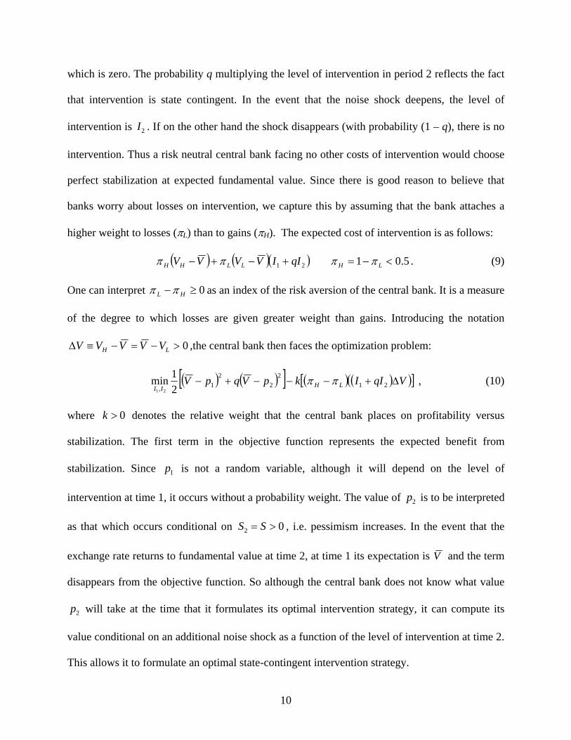
which is zero. The probability q multiplying the level of intervention in period 2 reflects the fact

that intervention is state contingent. In the event that the noise shock deepens, the level of

intervention is 2I . If on the other hand the shock disappears (with probability (1 – q), there is no

intervention. Thus a risk neutral central bank facing no other costs of intervention would choose

perfect stabilization at expected fundamental value. Since there is good reason to believe that

banks worry about losses on intervention, we capture this by assuming that the bank attaches a

higher weight to losses (πL) than to gains (πH). The expected cost of intervention is as follows:

( ) ( )( ) 5.01 21 <−=+−+− LHLLHH qIIVVVV ππππ . (9)

One 0≥− HL ππ as an index of the risk aversion of the central bank. It is a measure can interpret

of the degree to which losses are given greater weight than gains. Introducing the notation

0>−=−≡∆ LH VVVVV ,the central bank then faces the optimization problem:

( ) ( ) ] ( ) ( )( )[ ]VqIIkpVqp LH ∆+−−−+− 212

22

1 ππ , [VII , 2

1min21

(10)

wh tes the relative weight that the central bank places on profitability veere 0>k deno rsus

stabilization The first term in the objective function represents the expected benefit from

stabilization. Since 1p is not a random variable, although it will depend on the level of

intervention at time 1, it occurs without a probability weight. The value of 2p is to be interpreted

as that which occurs conditional on 02 >

.

= SS , i.e. pessimism increases. In the event that the

exchange rate returns to fundamental e 2, at time 1 its expectation is value at tim V and the term

disappears from the objective function. So although the central bank does not know what value

2p will take at the time that it formulates its optimal intervention strategy, it can compute its

ue conditional on an additional noise shock as a function of the level of intervention at time 2. val

This allows it to formulate an optimal state-contingent intervention strategy.

10

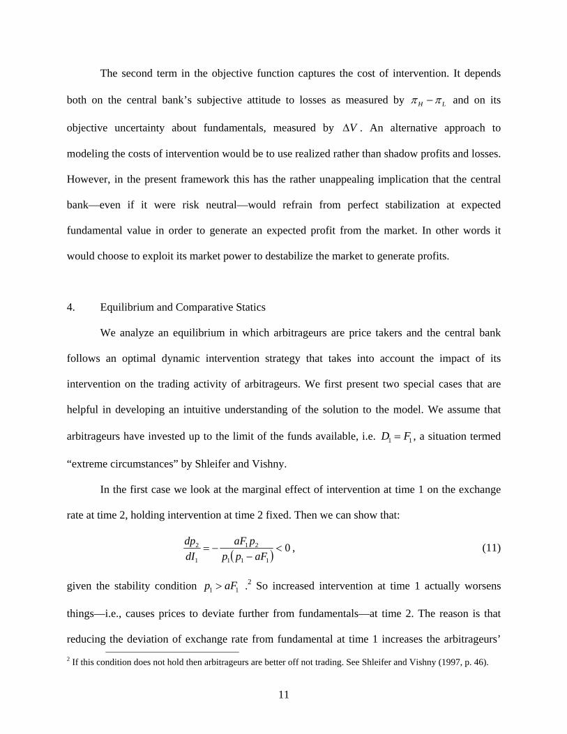
The second term in the objective function captures the cost of intervention. It depends

both on the central bank’s subjective attitude to losses as measured by LH ππ − and on its

objective uncertainty about fundamentals, measured by V∆ . An alternative approach to

modeling the costs of intervention would be to use realized rather than shadow profits and losses.

However, in the present framework this has the rather unapp ing implication that the central

bank—even if it were risk neutral—would refrain from perfect stabilization at expected

fundamental value in order to generate an expected profit from the market. In other words it

would choose to exploit its market power to destabilize the market to generate profits.

4. Equilibrium and Comparative Statics

eal

We analyze an equilibrium in which arbitrageurs are price takers and the central bank

rategy that takes into account the impact of its

terve

follows an optimal dynamic intervention st

in ntion on the trading activity of arbitrageurs. We first present two special cases that are

helpful in developing an intuitive understanding of the solution to the model. We assume that

arbitrageurs have invested up to the limit of the funds available, i.e. 11 FD = , a situation termed

“extreme circumstances” by Shleifer and Vishny.

In the first case we look at the marginal effect of intervention 1 on the exchange

rate at time 2, holding intervention at time 2 fixed.

at time

Then we can show that:

( ) 0111

21

1

2 <−=paFdp , (11) − aFppdI

given the stability condition .2 So increased intervention at time 1 actually worsens

things—i.e., causes prices to deviate further from fundamentals—at time 2. The reason is that

reducing the deviation of exchange rate from fundamental at time 1 increases the arbitrageurs’

11 aFp >

2 If this condition does not hold then arbitrageurs are better off not trading. See Shleifer and Vishny (1997, p. 46).

11

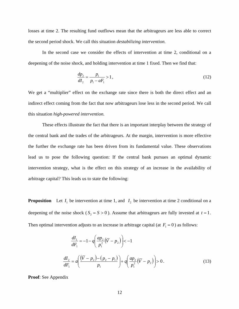
losses at time 2. The resulting fund outflows mean that the arbitrageurs are less able to correct

the second period shock. We call this situation destabilizing intervention.

In the second case we consider the effects of intervention at time 2, conditional on a

deepening of the noise shock, and holding intervention at time 1 fixed. Then we find that:

112 >=pdp ,

112 − aFpdI (12)

We get a “multiplier” effect on the exchange rate since there is both the direct effect and an

indirect effect coming from the fact that now arbitrageurs lose less in the second period. We call

this situati d intervention.

riven from its fundamental value. These observations

t arbitrageurs are fully invested at

on high-powere

These effects illustrate the fact that there is an important interplay between the strategy of

the central bank and the trades of the arbitrageurs. At the margin, intervention is more effective

the further the exchange rate has been d

lead us to pose the following question: If the central bank pursues an optimal dynamic

intervention strategy, what is the effect on this strategy of an increase in the availability of

arbitrage capital? This leads us to state the following:

Proposition Let 1I be intervention at time 1, and 2I be intervention at time 2 conditional on a

deepening of the noise shock ( 02 >= SS ). Assume tha 1=t .

hen optimal interventio an increase in arbitrage capital (at ) as follows:

n adjusts to 01 =FT

( ) 11 221

2

1 ⎠

⎞⎛ apdFdI

1 −<⎟⎟⎜⎜⎝

−−−= pVp

q

( ) ( ) ( ) 0221222 >⎟⎟

⎞⎜⎜⎛

−+⎟⎟⎞

⎜⎜⎛ −−−

= pVapqpppVadI 2111 ⎠⎝⎠⎝ ppdF

. (13)

Proof: See Appendix

12

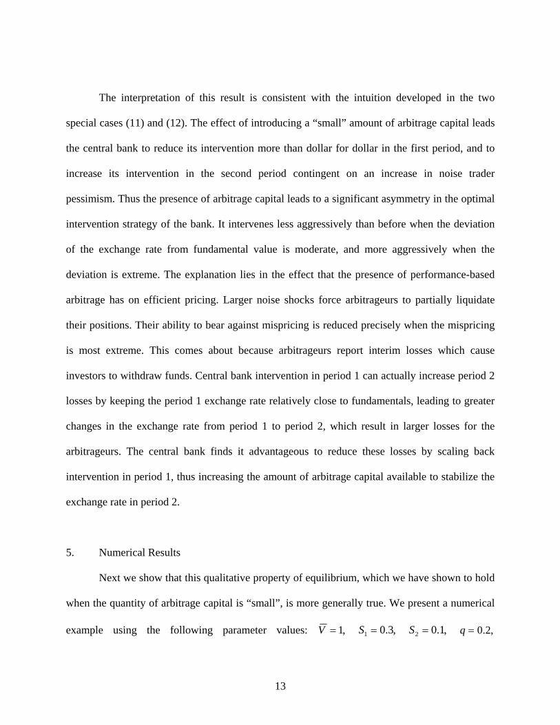
The interpretation of this result is consistent with the intuition developed in the two

special cases (11) and (12). The effect of introducing a “small” amount

the central bank to reduce its intervention more than dollar for dollar in the first period, and to

ion in the second period contingent on an increase in noise trader

essimism. Thus the presence of arbitrage capital leads to a significant asymmetry in the optimal

interve

wing parameter values:

of arbitrage capital leads

increase its intervent

p

ntion strategy of the bank. It intervenes less aggressively than before when the deviation

of the exchange rate from fundamental value is moderate, and more aggressively when the

deviation is extreme. The explanation lies in the effect that the presence of performance-based

arbitrage has on efficient pricing. Larger noise shocks force arbitrageurs to partially liquidate

their positions. Their ability to bear against mispricing is reduced precisely when the mispricing

is most extreme. This comes about because arbitrageurs report interim losses which cause

investors to withdraw funds. Central bank intervention in period 1 can actually increase period 2

losses by keeping the period 1 exchange rate relatively close to fundamentals, leading to greater

changes in the exchange rate from period 1 to period 2, which result in larger losses for the

arbitrageurs. The central bank finds it advantageous to reduce these losses by scaling back

intervention in period 1, thus increasing the amount of arbitrage capital available to stabilize the

exchange rate in period 2.

5. Numerical Results

Next we show that this qualitative property of equilibrium, which we have shown to hold

when the quantity of arbitrage capital is “small”, is more generally true. We present a numerical

example using the follo ,1=V ,3.01 =S ,1.02 =S ,2.0=q

13

,2.0=− HL ππ ,25.0=∆V =k 1.0 . Arbitrageurs always choose to be fully invested at 1=t

with these parameter values. In Figure 1 we fix a = 1.2, the parameter that governs the rate at

which funds are withdrawn when arbitrageurs make losses. For small values of 1F the central

bank intervenes more aggressively in period 1 than i o t

pite the fact that the incremental noise shock in period 2 is

considerably smaller than that in period 1.

In Figure 2 we fix 2.01 =F and allow a to vary. Increasing a shifts inte ention from

period 1 to period 2, as our earlier discussion would lead us to expect. That is, as PBA becomes

more important, the central bank intervenes less aggressively in period 1 – to reduce period 2

losses to arbitrageurs – and more aggressiv

n peri d 2. Bu as increases the

verses, des

ely in period 2. Note that the level of intervention in

period 2 shown in both figures is

1F

relationship eventually re

rv

contingent on an increase in the pessimism of noise traders. If

the exchange rate reverts to fundamental value at time 2 as a result of the early dissipation of

market pessimism, the central bank is able to close out its intervention position, so that 12 II −= .

This tendency of the central bank to intervene less when the importance of PBA increases

(a rises) explains why it is not optimal for the central bank to simply fully offset the noise shock

in the first period. As explained in the previous section, intervention in period 1 will increase

period 2 losses by keeping the period 1 exchange rate relatively close to fundamentals, leading to

greater changes in the exchange rate from period 1 to period 2, which result in larger losses for

the arbitrageurs.

Figure 3 illustrates the effect of simultaneous variation in 1F and a. Not surprisingly we

see that the effect of varying a becomes more pronounced as 1F increases. That is, larger

resources for arbitrageurs magnify the PBA effect on intervention.

14

th

n, so we would predict that

Our results provide a potential explanation for the fact that e frequency of intervention

has tended to decline over time, but the magnitude of interventions has increased.3 As the

quantity of arbitrage capital devoted to currency trading has rise

intervention when exchange rates deviate only to a moderate degree from fundamentals would

decline, whereas periods of extreme divergence would attract an increased volume of

intervention.

Finally, we can examine how the results would change if the central bank’s risk

aversion ( HL ππ − ) or the uncertainty about fundamentals ( V∆ ) increases. The value of k, the

weight in the central bank’s optimization function graphs subsumes both variables: An increase

mine ho

ave shown persistent

mis While volatile expectations seem to be a plausible theory as

to w

in k is equivalent to an increase in risk aversion or an increase in fundamental uncertainty. So,

we can exa w intervention in both periods changes as nction of k. Figure 4 duplicates

Figure 1, but for 3 different values of k, k = 0.1, 0.7, and 1.3. As k increases, intervention in

both periods tends to decline, but intervention in period 1 declines faster. At the same time, the

sensitivity of intervention in period 2 to 1F increases with the value of k.

6. Discussion and Conclusion

The behavior of the foreign exchange market has puzzled economists since the inception of

floating exchange rates in 1973. In particular, exchange rates appear to h

a fu

alignments with fundamentals.

hy exchange rates should deviate from long-run fundamentals, it is less clear why there is

not more risk-arbitrage on a return to long-term fundamentals. Shleifer and Vishny (1997)

3 For example, the U.S. authorities intervened 281 times from January 1, 1986 to January 1, 1996, but only twice since January 1, 1996. At the same time, the magnitude of a given intervention in the latter period was almost 5 times larger than an intervention in the former period. Similarly, the German authorities did not intervene from 1995 to the transition to the European Central Bank (ECB) in 1999. And the ECB has reportedly intervened sparingly since its inception.

15

provide at least a partial answer by pointing out some problems associated with assuming that

rational risk-arbitrage will quickly drive asset prices back to long-run equilibrium. In particular,

they show that “performance-based asset management” may generate situations in which asset

price disequilibrium will worsen, before being corrected. This in turn limits the effect of rational

risk-arbitrage.

This paper extends the Shleifer and Vishny (1997) model to include central bank

intervention and fundamental uncertainty. Our results indicate that increasing availability of

arbitrage capital has a pronounced effect on the dynamic intervention strategy of the central

ust 1998,

bank. Intervention is reduced during periods of moderate misalignment and amplified at times of

extreme misalignment. This pattern is consistent with empirical observation. We show also that

the central bank’s uncertainty about the true fundamental value of the exchange rate and its

aversion to the risk of making losses are factors that will limit its intervention activity.

It is worth noting that the logic of our argument is not confined to the foreign exchange

market. But it is certainly true that episodes in which monetary authorities have intervened to

influence the stock market are much less common. One such occurrence was in Aug

when the Hong Kong Monetary Authority purchased HK$118 billion in shares in the 33 large

capitalization stocks of the Hang-Seng Index over a period of ten days (Bhanot and

Kadapakkam, 2004). This was a massive intervention, representing roughly twenty times the

average daily trading volume on the Hong Kong market. To the extent that extreme deviations

from fundamentals are less common in a stock market index than in the market for foreign

exchange, and that more private capital is devoted to arbitrage in the stock market, our model

provides a possible explanation for the difference in observed frequency of intervention, and for

16

the fact that when such interventions do take place in the stock market, they are particularly

large.

A primary longer-term goal of any research program that seeks to understand the

intervention behavior of central banks will need to explain the diminishing appetite for such

intervention. The increasing importance of private sector risk-arbitrage, the diminishing ratio of

intervention resources to trading volume, and greater reliance on verbal interventions may be

important factors in modeling this trend.

17

References

Barberis, N., and R. Thaler. “A Survey of Behavioral Finance.” National Bureau of Economic Research, Inc., 2002, NBER Working Paper: 9222.

Bhanot, K., and K. Palani-Rajan. “Anatomy of a Government Intervention in Index Stocks – Price Pressure or Information Effects?” Journal of Business, 2004, 79(2), pp. 963-86.

Brav, A., J.B. Heaton, and A. Rosenberg. “The Rational-Behavioral Debate in Financial Economics.” Journal of Economic Methodology, 2004, 11(4), pp. 393-409.

Brunnermeier, M.K., and S. Nagel. “Hedge Funds and the Technology Bubble.” Journal of Finance, 2004, 59(5), pp. 2013-40.

Collins, D.W., G. Gong, and P. Hribar. “Investor Sophistication and the Mispricing of Accruals.” Review of Accounting Studies, 2003, 8(2-3), pp. 251-76.

DeLong, J.B., A. Shleifer, L. Summers and R.J. Waldmann. “Noise trader risk in financial markets.” Journal of Political Economy, 1990, 98(4), pp. 703-38.

Devereux, M.B., and C. Engel. “Exchange Rate Pass-Through, Exchange Rate Volatility, and Exchange Rate Disconnect.” Journal of Monetary Economics, 2002, 49(5), pp. 913-40.

Duarte, M., and A.C. Stockman. “Rational Speculation and Exchange Rates.” National Bureau of Economic Research, Inc, 2001, NBER Working Paper: 8362.

Duarte, M., and A.C. Stockman. “Comment on: Exchange rate pass-through, exchange rate volatility, and exchange rate disconnect.” Journal of Monetary Economics, 2002, 49(5), pp. 941–46.

Engel, C. "The Forward Discount Anomaly and the Risk Premium: A Survey of Recent Evidence." Journal of Empirical Finance, 1996, 3(2), pp. 123-192.

Engel, C. “Long-Run PPP May Not Hold After All.” Journal of International Economics, 2000, 51(2), pp. 243-73.

Frankel, J. “How Well Do Foreign Exchange Markets Function: Might a Tobin Tax Help?” National Bureau of Economic Research, Inc., 1996, NBER Working Paper: 5422.

Frankel, J.A., and K.A. Froot. “Using Survey Data to Test Standard Propositions Regarding Exchange Rate Expectations.” American Economic Review, 1987, 77(1), pp. 133-53.

Gabaix, X., A. Krishnamurthy, and O. Vigneron. “Limits of Arbitrage: Theory and Evidence from the Mortgage-Backed Securities Market.” National Bureau of Economic Research, Inc., 2005, NBER Working Paper: 11851.

18

Gallagher, L.A., and M.P. Taylor. “Risky Arbitrage, Limits of Arbitrage, and Nonlinear Adjustment in the Dividend-Price Ratio.” Economic Inquiry, 2001, 39(4), pp. 524-36.

Greenwood, R. “Short- and Long-Term Demand Curves for Stocks: Theory and Evidence on the Dynamics of Arbitrage.” Journal of Financial Economics, 2005, 75(3), pp. 607-49.

Hodrick, R.J. “The Empirical Evidence on the Efficiency of Forward and Futures Foreign Exchange Markets.” In Fundamentals of Pure and Applied Economics, 1987, vol. 24, Lesourne, J., and H. Sonnenschein (eds)., Harwood: New York.

Jiang, G., M.C. Lee, and Y. Zhang. “Information Uncertainty and Expected Returns.” Review of Accounting Studies, 2005, 10(2-3), pp. 185-221.

Kilian, L. “Exchange Rates and Monetary Fundamentals: What Do We Learn from Long-Horizon Regressions?” Journal of Applied Econometrics, 1999, 14(5), pp. 491-510.

Krugman, P., and M. Miller. “Why Have a Target Zone?” Carnegie-Rochester Conference Series on Public Policy, 1993, 38, pp. 279-314.

Leahy, M.P. “The Profitability of U.S. Intervention in the Foreign Exchange Markets.” Journal of International Money and Finance, 1995, 14(6), pp. 823-44.

Mark, N., and D. Sul. “Nominal Exchange Rates and Monetary Fundamentals: Evidence from a Small Post-Bretton Woods Panel.” Journal of International Economics, 2001, 53(1), pp. 29-52.

Massa, M., U. Peyer, and Z. Tong. “Limits of Arbitrage and Corporate Financial Policy.” C.E.P.R. Discussion Papers, 2005, CEPR Discussion Paper: 4829.

McMillan, D.G. “Non-linear Dynamics in International Stock Market Returns.” Review of Financial Economics, 2005, 14(1), pp. 81-91.

Meese, R.A., and K. Rogoff. “Empirical Exchange Rate Models of the Seventies: Do They Fit Out of Sample?” Journal of International Economics, 1983, 14(1-2), pp. 3-24.

Meredith, G., and M. Chinn. “Long-Horizon Uncovered Interest Rate Parity.” National Bureau of Economic Research, Inc., 1998, NBER Working Paper: 6797.

Mussa, M. “Nominal Exchange Rate Regimes and the Behavior of Real Exchange Rates: Evidence and Implications.” In Carnegie-Rochester, Conference Series on Public Policy: Real Business Cycles, Real Exchange Rates, and Actual Policies, 1986, vol. 25, K. Bruner, and A.H. Meltzer (eds)., pp. 117-214.

Neely, C.J. “Technical Analysis in the Foreign Exchange Market: A Layman’s Guide.” Federal Reserve Bank of St. Louis Review, 1997, 79(5), pp. 23-38.

Neely, C.J. “Technical Analysis and the Profitability of U.S. Foreign Exchange Intervention.” Federal Reserve Bank of St. Louis Review, 1998, 80(4), pp. 3-17.

19

Neely, C.J. “The Case for Foreign Exchange Intervention: The Government as an Active Reserve Manager.” Federal Reserve Bank of St. Louis Working Paper, 2005, Working Paper: 2004-031B.

Neely, C.J., and L. Sarno. “How Well Do Monetary Fundamentals Forecast Exchange Rates?” Federal Reserve Bank of St. Louis Review, 2002, 84(5), pp. 51-74.

Neely, C.J., P.A. Weller, and R.D. Dittmar. “Is technical analysis in the foreign exchange market profitable? A genetic programming approach.” Journal of Financial and Quantitative Analysis, 1997, 32(4), pp. 405–26.

Rapach, D.E., and M.E. Wohar. “Testing the Monetary Model of Exchange Rate Determination: New Evidence from a Century of Data.” Journal of International Economics, 2002, 58(2), pp. 359-85.

Sarno, L., and M.P. Taylor. “The Microstructure of the Foreign Exchange Market: A Selective Survey of the Literature.” Princeton Studies in International Economics, 2001, No. 89.

Shleifer, A., and R.W. Vishny. “The Limits of Arbitrage.” Journal of Finance, 1997, 52(1), pp. 35-55.

Sjöö, B., and R.J. Sweeney. “The Foreign-Exchange Costs of Central Bank Intervention: Evidence from Sweden.” Journal of International Money and Finance, 2001, 20(2), pp. 219-47.

Stein, J.C. “Why Are Most Funds Open-End? Competition and the Limits of Arbitrage.” Quarterly Journal of Economics, 2005, 120(1), pp. 247-72.

Sweeney, R.J. “Beating the foreign exchange market.” Journal of Finance, 1986, 41(1), pp. 163-82.

Sweeney, R.J. “Do Central Banks Lose on Foreign-Exchange Intervention? A Review Article.” Journal of Banking and Finance, 1997, 21(11-12), pp. 1667-84.

20

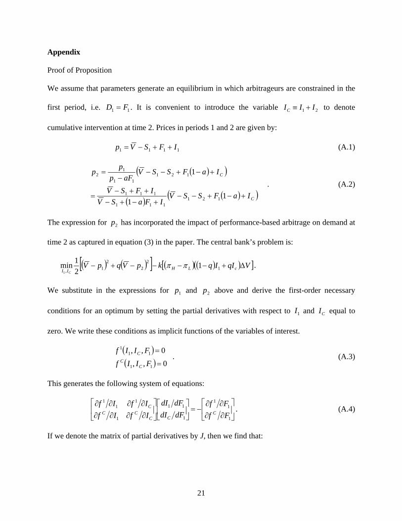
Appendix

Proof of Proposition

We assume that parameters generate an equilibrium in which arbitrageurs are constrained in the

first period, i.e. . It is convenient to introduce the variable to denote

cumulative intervention at time 2. Prices in periods 1 and 2 are given by:

11 FD = 21 IIIC +≡

1111 IFSVp ++−= (A.1)

( )( )

( ) ( )( )C

C

IaFSSVIFaSV

IFSV

IaFSSVaFp

pp

+−+−−+−+−

++−=

+−+−−−

=

11

1

121111

111

12111

12

. (A.2)

The expression for has incorporated the impact of performance-based arbitrage on demand at

time 2 as captured in equation (3) in the paper. The central bank’s problem is:

2p

( ) ( )[ ] ( ) ( )( )[ ]VqIIqkpVqpV cLHII C

∆+−−−−+− 12

22

1,1

21min

1

ππ .

We substitute in the expressions for and above and derive the first-order necessary

conditions for an optimum by setting the partial derivatives with respect to and equal to

zero. We write these conditions as implicit functions of the variables of interest.

1p 2p

1I CI

. (A.3) ( )( ) 0,,

0,,

11

111

=

=

FIIf

FIIf

CC

C

This generates the following system of equations:

⎥⎦

⎤⎢⎣

⎡

∂∂∂∂

−=⎥⎦

⎤⎢⎣

⎡⎥⎦

⎤⎢⎣

⎡

∂∂∂∂∂∂∂∂

1

11

1

11

1

11

1

FfFf

dFdIdFdI

IfIfIfIf

CCC

CCC . (A.4)

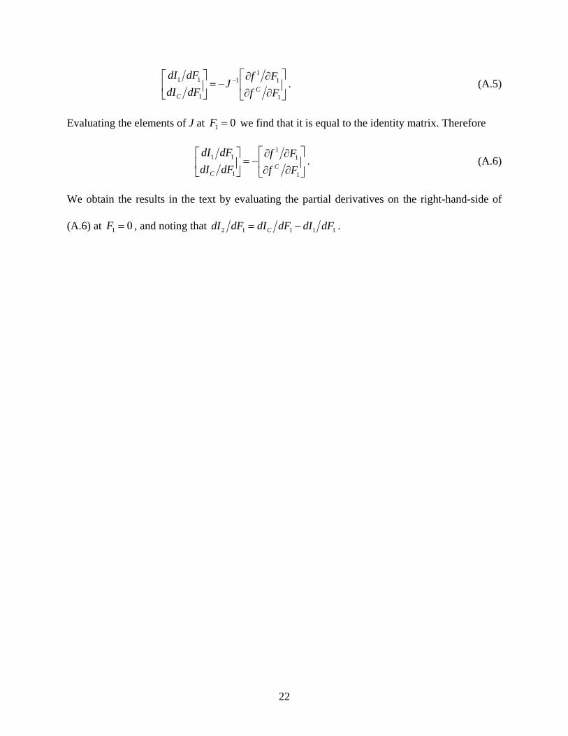
If we denote the matrix of partial derivatives by J, then we find that:

21

⎥⎦

⎤⎢⎣

⎡

∂∂∂∂

−=⎥⎦

⎤⎢⎣

⎡ −

1

11

1

1

11

FfFf

JdFdIdFdI

CC

. (A.5)

Evaluating the elements of J at we find that it is equal to the identity matrix. Therefore 01 =F

⎥⎦

⎤⎢⎣

⎡

∂∂∂∂

−=⎥⎦

⎤⎢⎣

⎡

1

11

1

11

FfFf

dFdIdFdI

CC

. (A.6)

We obtain the results in the text by evaluating the partial derivatives on the right-hand-side of

(A.6) at , and noting that 01 =F 11112 dFdIdFdIdFdI C −= .

22

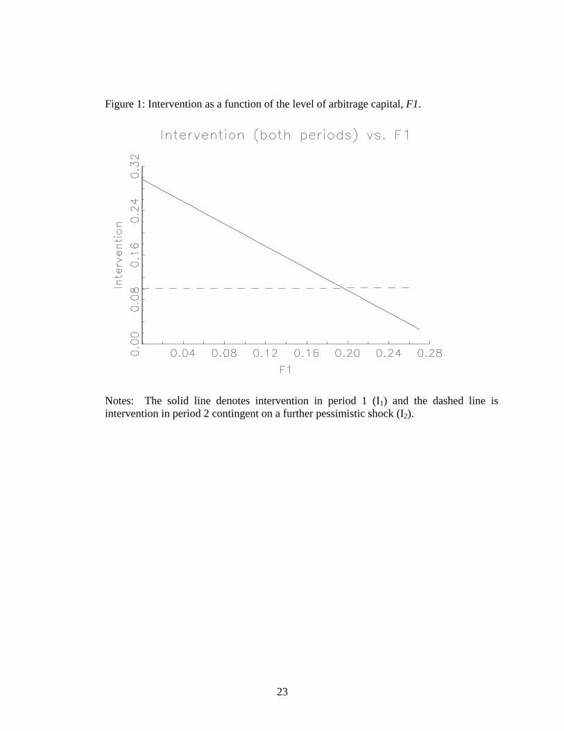
Figure 1: Intervention as a function of the level of arbitrage capital, F1.

Notes: The solid line denotes intervention in period 1 (I1) and the dashed line is intervention in period 2 contingent on a further pessimistic shock (I2).

23

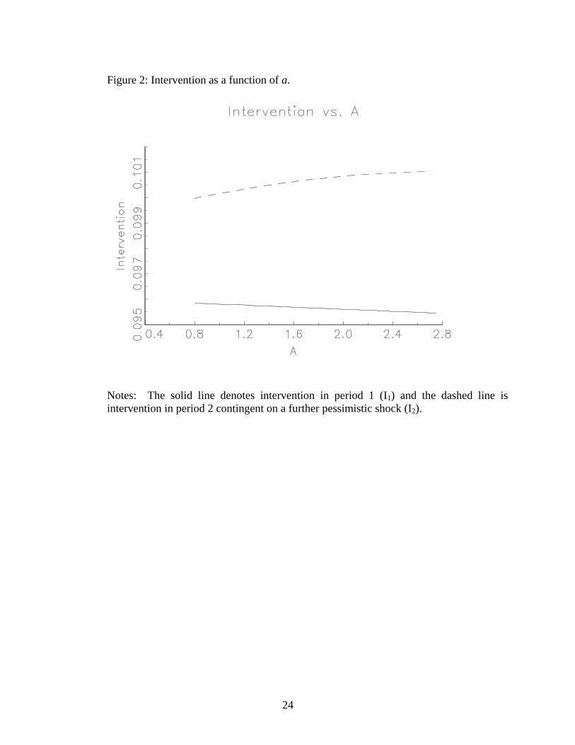
Figure 2: Intervention as a function of a.

Notes: The solid line denotes intervention in period 1 (I1) and the dashed line is intervention in period 2 contingent on a further pessimistic shock (I2).

24

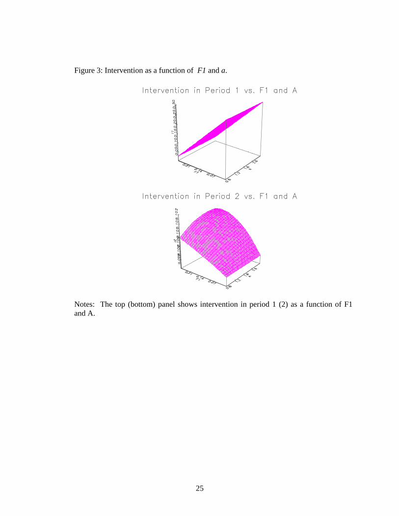
Figure 3: Intervention as a function of F1 and a.

Notes: The top (bottom) panel shows intervention in period 1 (2) as a function of F1 and A.

25

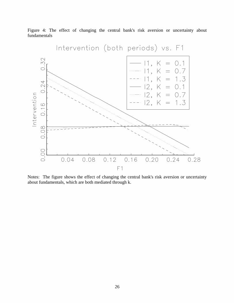
Figure 4: The effect of changing the central bank's risk aversion or uncertainty about fundamentals

Notes: The figure shows the effect of changing the central bank's risk aversion or uncertainty about fundamentals, which are both mediated through k.

26