cellular network - university of pittsburgh

5. CELLULAR WIRELESS NETWORK

CS-1699 Wireless NetworksTerm : Spring 2018

Instructor : Xerandy

CELLULAR NETWORKS

• Revolutionary development in data communications and telecommunications

• Foundation of mobile wireless– Telephones, smartphones, tablets, wireless Internet, wireless

applications• Supports locations not easily served by wireless networks

or WLANs• Four generations of standards

– 1G: Analog– 2G: Still used to carry voice– 3G: First with sufficient speeds for data networking, packets only– 4G: Truly broadband mobile data up to 1 Gbps

Cellular Wireless Networks 13-2

CELLULAR NETWORK ORGANIZATION

• Use multiple low-power transmitters (100 W or less)

• Areas divided into cells– Each served by its own antenna

– Served by base station consisting of transmitter, receiver, and control unit

– Band of frequencies allocated

– Cells set up such that antennas of all neighbors are equidistant (hexagonal pattern)• Idealized pattern, in order to approximate coverage


CELLULAR NETWORK ORGANIZATION

• Why not a large service area– Number of simultaneous user to serve would be

limited– Mobile handset needs to have larger power

requirement• Smaller cells

– Allows frequency reuse, hence increased capacity for the same area of coverage

– Lower power handset– Cons : Cost of cells, hands off between cells must be

supported, need to track user to route incoming call or message.

13.1 CELLULAR GEOMETRIESCellular Wireless Networks 13-5

FREQUENCY REUSE

• Adjacent cells assigned different frequencies to avoid interference or crosstalk

• Objective is to reuse frequency in nearby cells– 10 to 50 frequencies assigned to each cell

– Transmission power controlled to limit power at that frequency escaping to adjacent cells

– The issue is to determine how many cells must intervene between two cells using the same frequency


13.2 FREQUENCY REUSE PATTERNSCellular Wireless Networks 13-7

FREQUENCY REUSE

• D= Minimum distance between center of cells that use the same frequency band (called co-channels)

• R=Radius of a cell• d=Distance between centers of adjacent cells

– Relation :

• N=Number of cells in a repetitious pattern (each cell in the pattern uses a unique hexagonal geometry)– Possible N : , where I,J=0,1,2,3…

– Following relation holds : and

CELLULAR CONCEPT

• (N=7, where I=2, and J=1). Move I cells along any chain of hexagons, and turn 60 degrees ccw and move J steps

A

A

I steps

J steps 60 degrees

D

APPROACHES TO COPE WITH INCREASING CAPACITY

• Adding new channels• Frequency borrowing – frequencies are taken from adjacent

cells by congested cells• Cell splitting – cells in areas of high usage can be split into

smaller cells• Cell sectoring – cells are divided into a number of wedge-

shaped sectors, each with their own set of channels• Network densification – more cells and frequency reuse

– Microcells – antennas move to buildings, hills, and lamp posts– Femtocells – antennas to create small cells in buildings

• Interference coordination – tighter control of interference so frequencies can be reused closer to other base stations– Inter-cell interference coordination (ICIC)– Coordinated multipoint transmission (CoMP)


13.3 CELL SPLITTINGCellular Wireless Networks 13-11

INCREASING CAPACITY EXAMPLE

• If a cellular system supports K channels, and reuse factor is N (or the number of cells in every unique pattern), then

– Number channel per-cell is defined as

• Example

Width=11 x 1.6km=17.6 km

Wid

th=5

×3

×1

.6 𝑘

𝑚 =

13.

9 km

Wid

th=1

0×

3×

0.8

𝑘𝑚

= 1

3.9

km

Width=21 x 0.8 km=16.8 km

INCREASING CAPACITY EXAMPLE

• Given : Number of total channel K : 336 channels, reuse factor N=7.– (Left figure) R=1.6 km, number of cell : 32 cells

Each cell has area of Total coverage area =

Number of channel per cell,

Total channel capacity

– (Right figure). R=0.8 km Each cell has area of

To cover 213 km, number of cells would be .

128 cells

Number of channel per cell,

Total channel capacity

CELLULAR SYSTEMS TERMS

• Base Station (BS) – includes an antenna, a controller, and a number of receivers

• Mobile telecommunications switching office (MTSO) – connects calls between mobile units

• Two types of channels available between mobile unit and BS– Control channels – used to exchange information having to

do with setting up and maintaining calls– Traffic channels – carry voice or data connection between

users


13.5 OVERVIEW OF CELLULAR SYSTEMCellular Wireless Networks 13-15

STEPS IN AN MTSO CONTROLLED CALL BETWEEN MOBILE USERS

• Mobile unit initialization

• Mobile-originated call

• Paging

• Call accepted

• Ongoing call

• Handoff


13.6 EXAMPLE OF MOBILE CELLULAR CALLCellular Wireless Networks 13-17

ADDITIONAL FUNCTIONS IN AN MTSO CONTROLLED CALL

• Call blocking

• Call termination

• Call drop

• Calls to/from fixed and remote mobile subscriber


MOBILE RADIO PROPAGATION EFFECTS

• Signal strength– Must be strong enough between base station and mobile

unit to maintain signal quality at the receiver– Must not be so strong as to create too much co-channel

interference with channels in another cell using the same frequency band

• Fading– Signal propagation effects may disrupt the signal and cause

errors


FREE SPACE LOSS

• Free space loss, ideal isotropic antenna

• Pt = signal power at transmitting antenna

• Pr = signal power at receiving antenna

• λ = carrier wavelength

• d = propagation distance between antennas

• c = speed of light (3 ×108 m/s)

where d and λ are in the same units (e.g., meters)

The Wireless Channel 6-20

Pt

Pr

=4pd( )2

l2=

4p fd( )2

c2

FREE SPACE LOSS

• Free space loss equation can be recast:


L

dB=10log

Pt

Pr

=20log4pdl

æ

èçö

ø÷

( ) ( ) dB 98.21log20log20 = dl

( ) ( ) dB 56.147log20log204

log20 =÷øö

çèæ= df

c

fdp

PATH LOSS EXPONENT IN PRACTICAL SYSTEMS

• Practical systems – reflections, scattering, etc.

• Beyond a certain distance, received power decreases logarithmically with distance– Based on many measurement studies

Pt

Pr

=4pl

æèç

öø÷

2

d n =4pf

c

æèç

öø÷

2

d n

L

dB= 20log f( ) 10n log d( ) 147.56 dB


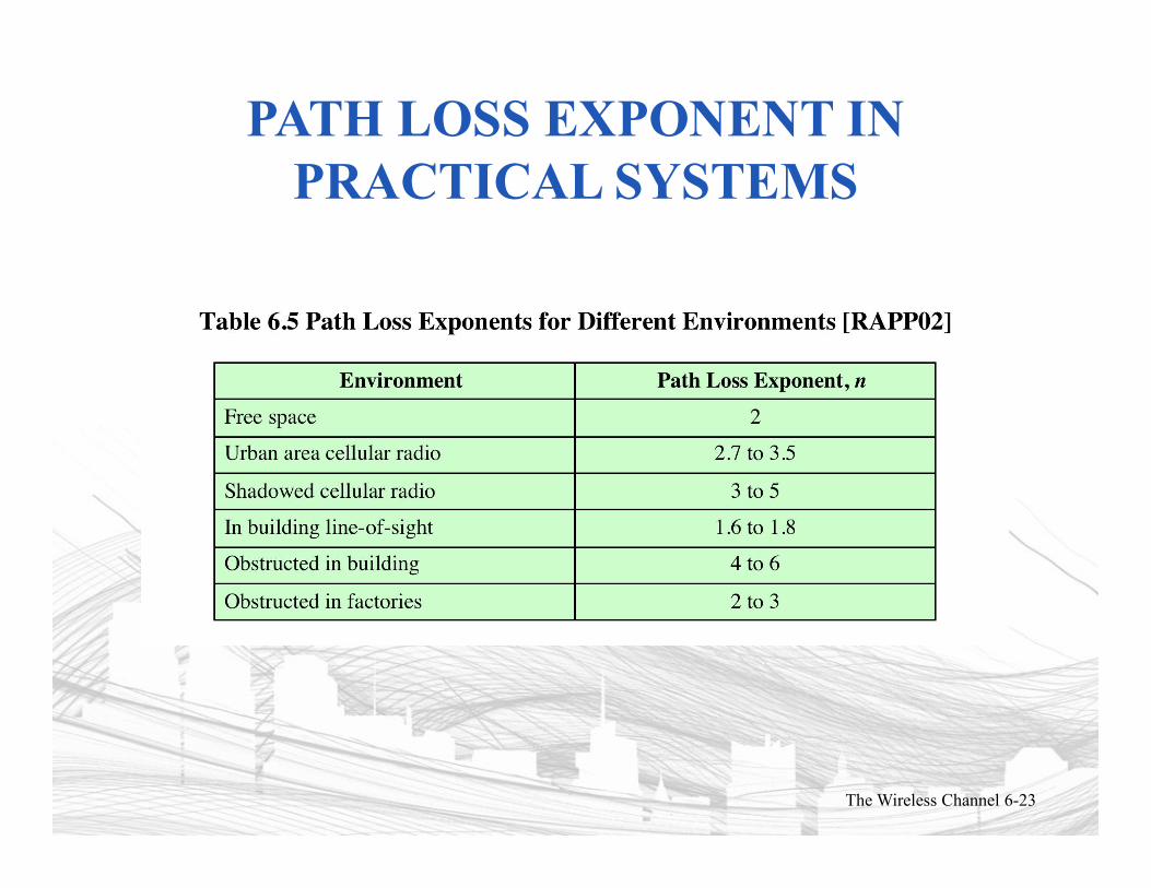
PATH LOSS EXPONENT IN PRACTICAL SYSTEMS


MODELS DERIVED FROM EMPIRICAL MEASUREMENTS

• Need to design systems based on empirical data applied to a particular environment– To determine power levels, tower heights, height of mobile

antennas• Okumura developed a model, later refined by Hata

– Detailed measurement and analysis of the Tokyo area– Among the best accuracy in a wide variety of situations

• Predicts path loss for typical environments– Urban– Small, medium sized city– Large city– Suburban– Rural


OKUMURA-HATA MODEL

• = carrier frequency in MHz, from 150 to 1500 MHz

• = height of base station antenna, in m, from 30 to 300 meter

• =height of receiving antenna(mobile unit), in m, from 1 to 10 m

• d= propagation distance between antenna in km, from 1 to 20 km

• = correction factor for mobile unit antenna height

d

Path loss in urban environment, predicted path loss based on Okumura Hata is :

OKUMURA-HATA MODEL

• Correction factor – Small of medium-sized city

dB

– For large citydB for

dB for

OKUMURA HATA MODEL

• Path loss for sub urban area :

dB

• Path loss in open or rural area:

OKUMURA HATA

• Example– Let =900 MHz, =40m, =5 m, and d=10 km.

Estimate the path loss for medium sized city, urban area=12.75-3.8 =8.95 dB

=69.55+26.16 -8.95

+(44.9-6.55 ) (10)=150.14 dB

cellular network - university of pittsburgh

Documents