cellular automata: tutorial - grlmc · cellular automata: tutorial jarkko kari department of...
TRANSCRIPT
Cellular Automata: Tutorial
Jarkko Kari
Department of Mathematics, University of Turku, Finland
TUCS(Turku Centre for Computer Science), Turku, Finland
Cellular Automata: examples
A Cellular Automaton (CA) is an infinite, regular lattice of
simple finite state machines that change their states
synchronously, according to a local update rule that specifies
the new state of each cell based on the old states of its
neighbors.
Cellular Automata: examples
A Cellular Automaton (CA) is an infinite, regular lattice of
simple finite state machines that change their states
synchronously, according to a local update rule that specifies
the new state of each cell based on the old states of its
neighbors.
The most widely known example is the Game-of-Life by
John Conway. It is a two-dimensional CA which means that
the space is an infinite checker-board. Each cell (=square of
the checker-board) has two possible states, ”Alive” and
”Dead”, represented by drawing the corresponding square
black or white, respectively.
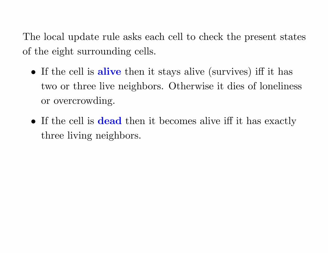
The local update rule asks each cell to check the present states
of the eight surrounding cells.
• If the cell is alive then it stays alive (survives) iff it has
two or three live neighbors. Otherwise it dies of loneliness
or overcrowding.
The local update rule asks each cell to check the present states
of the eight surrounding cells.
• If the cell is alive then it stays alive (survives) iff it has
two or three live neighbors. Otherwise it dies of loneliness
or overcrowding.
• If the cell is dead then it becomes alive iff it has exactly
three living neighbors.
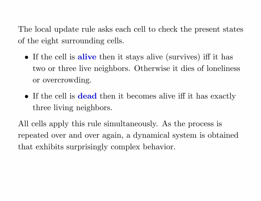
All cells apply this rule simultaneously. As the process is
repeated over and over again, a dynamical system is obtained
that exhibits surprisingly complex behavior.

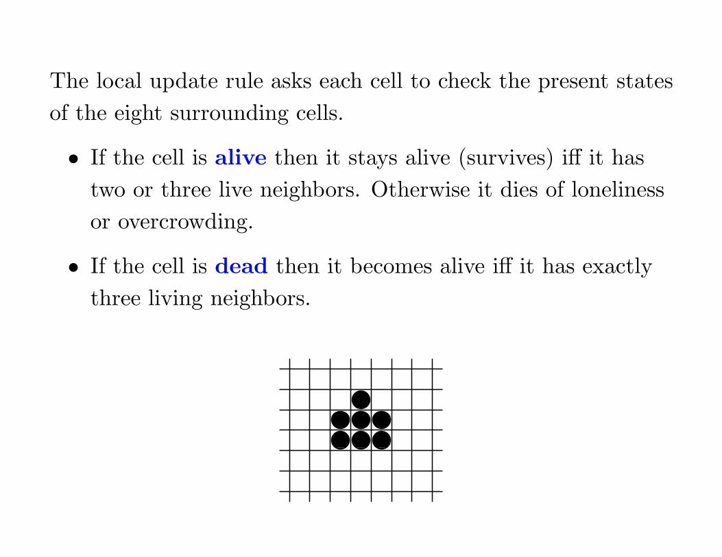
The local update rule asks each cell to check the present states
of the eight surrounding cells.
• If the cell is alive then it stays alive (survives) iff it has
two or three live neighbors. Otherwise it dies of loneliness
or overcrowding.
• If the cell is dead then it becomes alive iff it has exactly
three living neighbors.
������
������
������
������
������
������
������
������
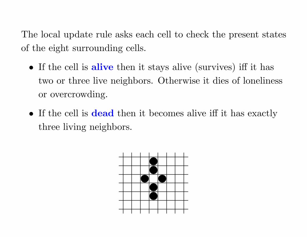
The local update rule asks each cell to check the present states
of the eight surrounding cells.
• If the cell is alive then it stays alive (survives) iff it has
two or three live neighbors. Otherwise it dies of loneliness
or overcrowding.
• If the cell is dead then it becomes alive iff it has exactly
three living neighbors.
������
������
������
������
������
������
������
������������
������
������
������
������
������

The local update rule asks each cell to check the present states
of the eight surrounding cells.
• If the cell is alive then it stays alive (survives) iff it has
two or three live neighbors. Otherwise it dies of loneliness
or overcrowding.
• If the cell is dead then it becomes alive iff it has exactly
three living neighbors.
������
������
������
������
������
������
������
������
������
������
������
������
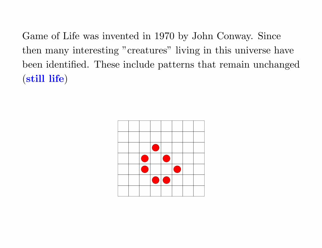
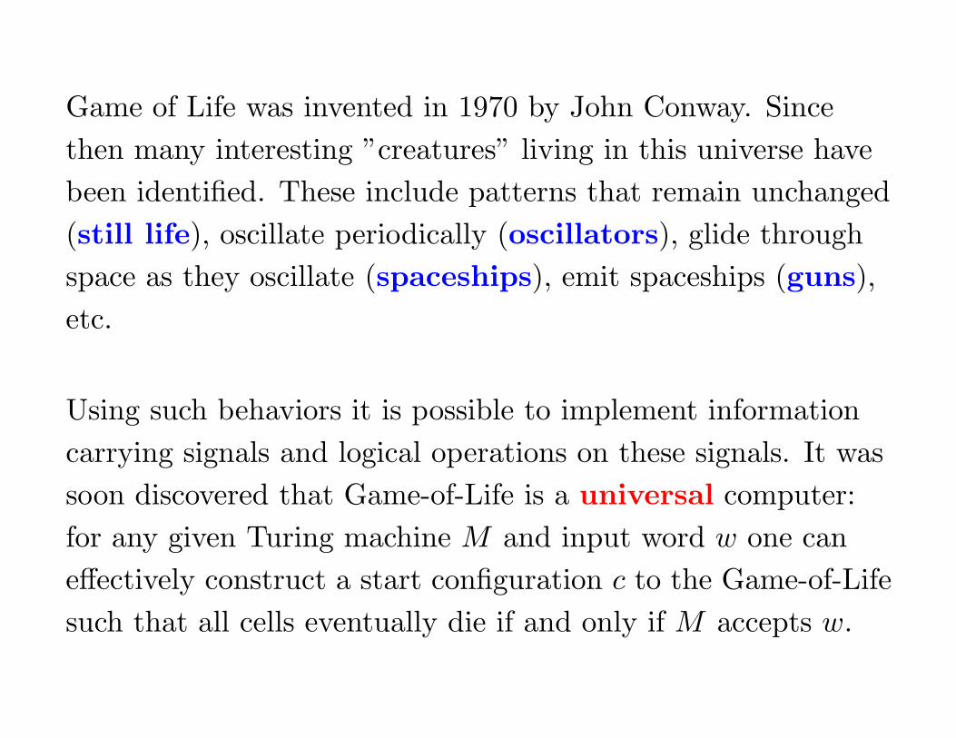
Game of Life was invented in 1970 by John Conway. Since
then many interesting ”creatures” living in this universe have
been identified. These include patterns that remain unchanged
(still life)
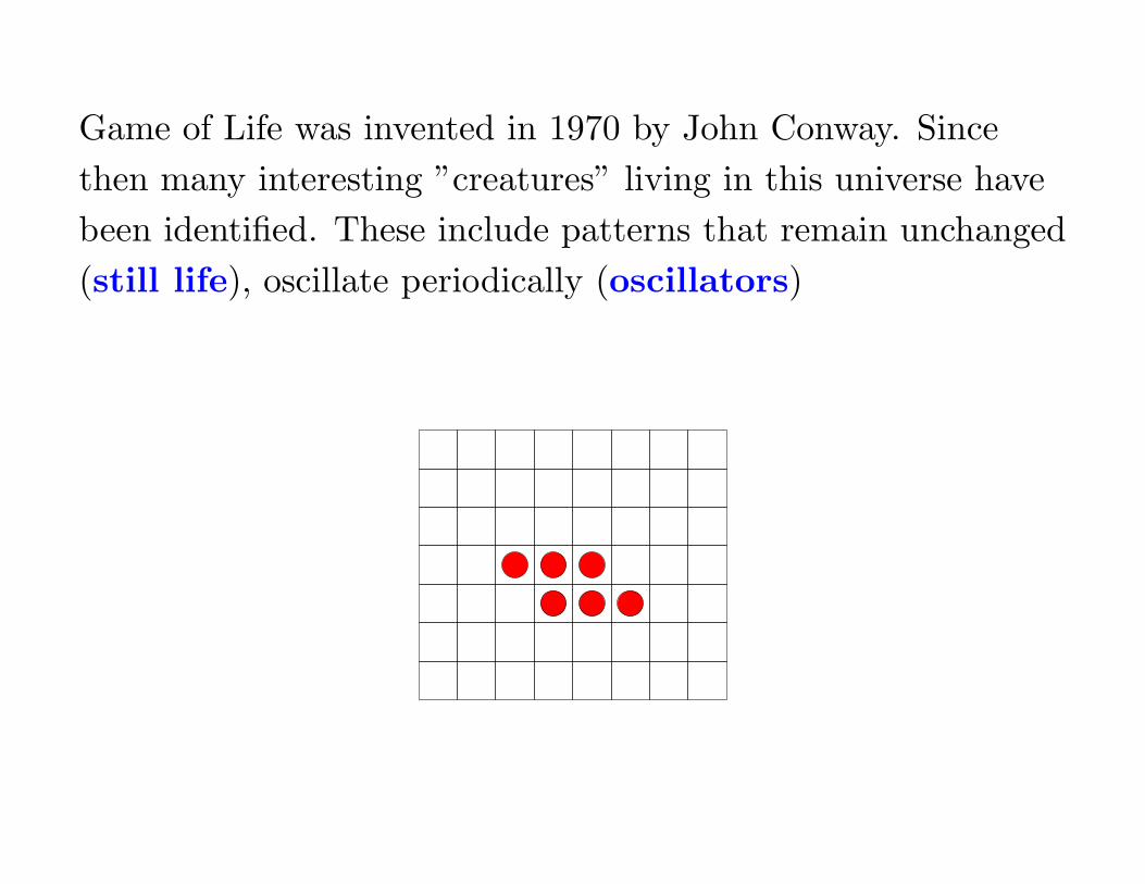
Game of Life was invented in 1970 by John Conway. Since
then many interesting ”creatures” living in this universe have
been identified. These include patterns that remain unchanged
(still life), oscillate periodically (oscillators)
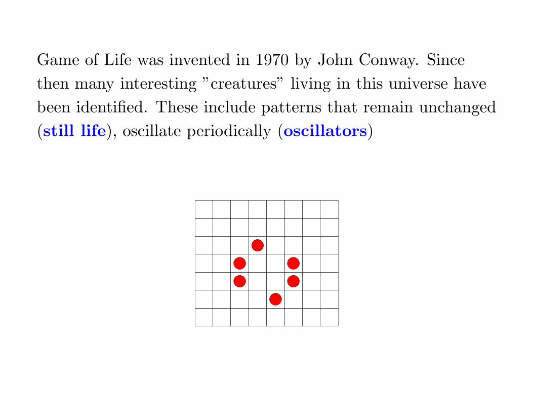
Game of Life was invented in 1970 by John Conway. Since
then many interesting ”creatures” living in this universe have
been identified. These include patterns that remain unchanged
(still life), oscillate periodically (oscillators)
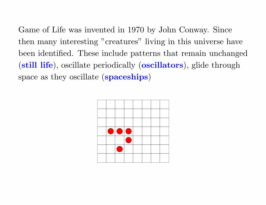
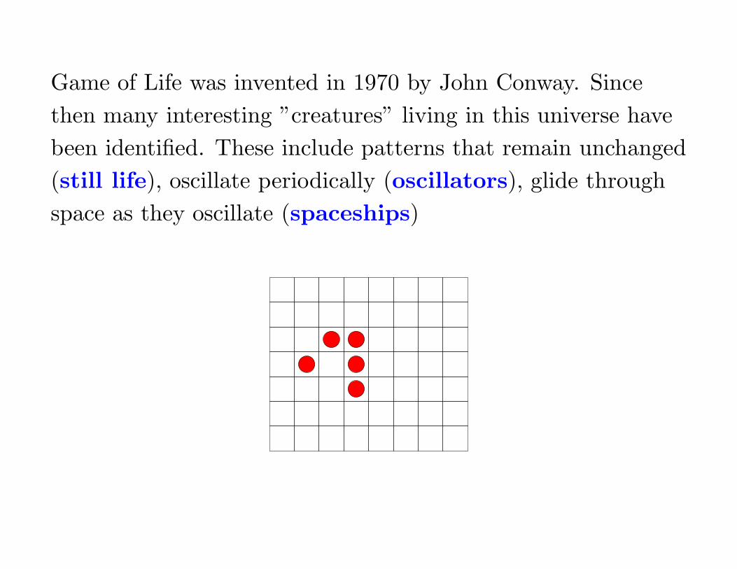
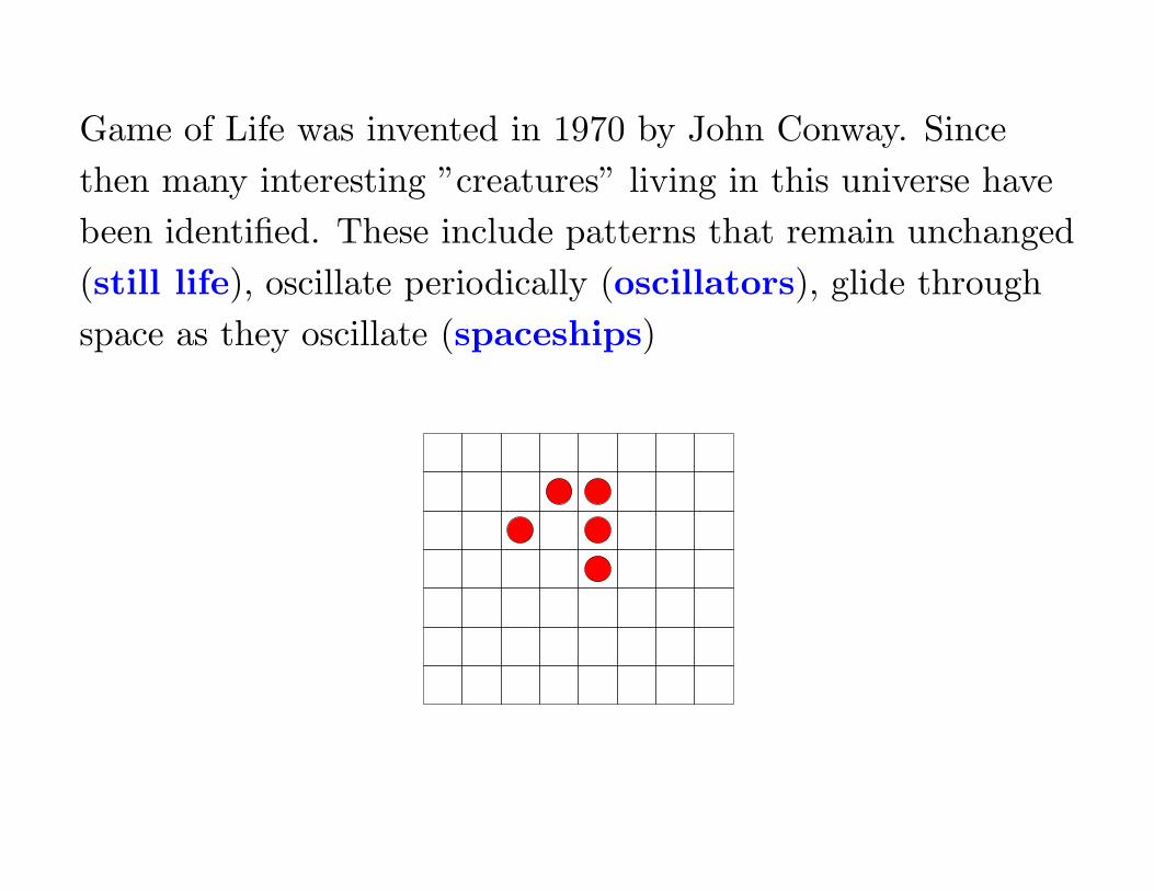
Game of Life was invented in 1970 by John Conway. Since
then many interesting ”creatures” living in this universe have
been identified. These include patterns that remain unchanged
(still life), oscillate periodically (oscillators), glide through
space as they oscillate (spaceships)

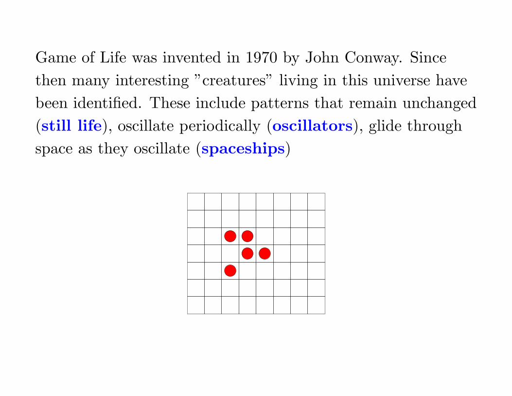
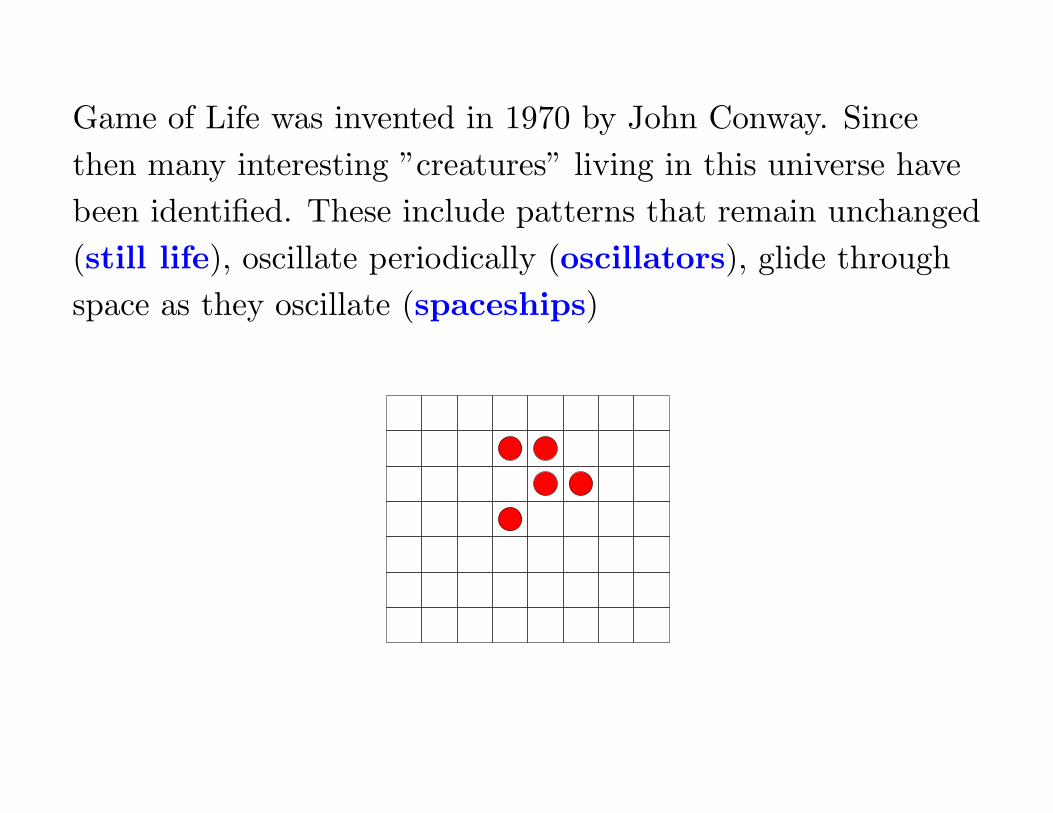
Game of Life was invented in 1970 by John Conway. Since
then many interesting ”creatures” living in this universe have
been identified. These include patterns that remain unchanged
(still life), oscillate periodically (oscillators), glide through
space as they oscillate (spaceships)
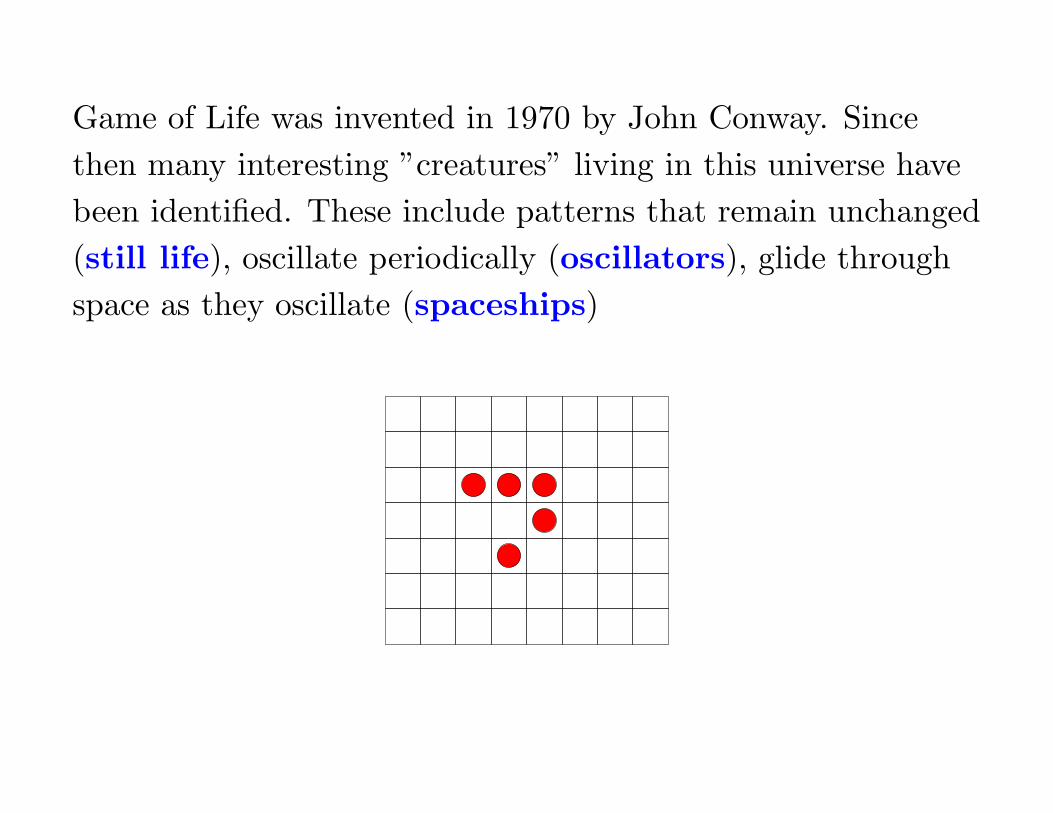
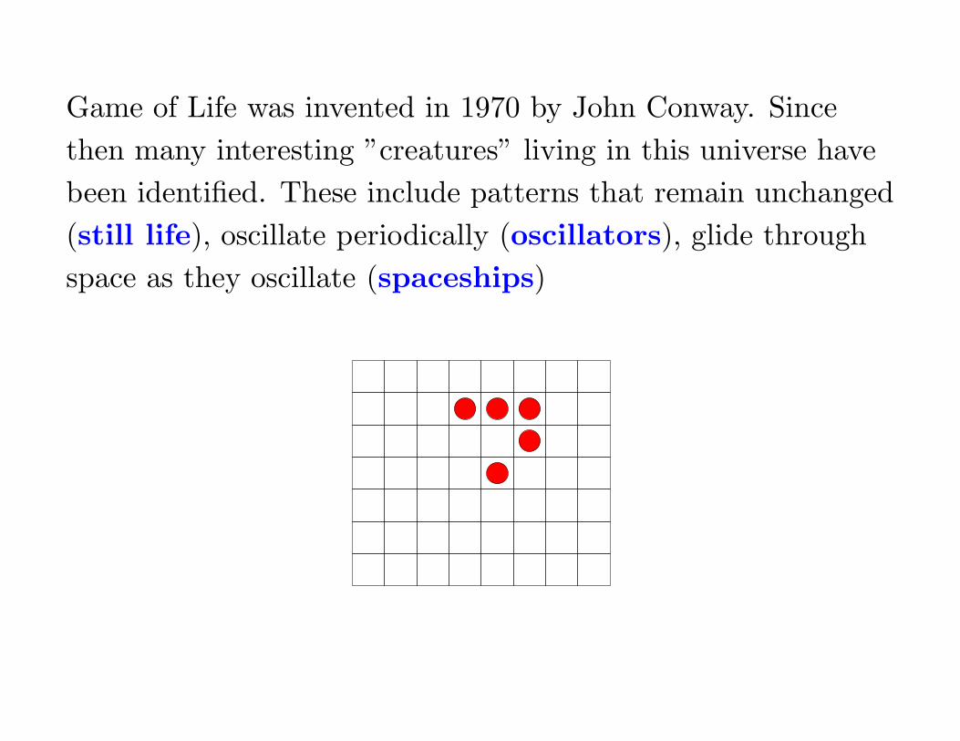
Game of Life was invented in 1970 by John Conway. Since
then many interesting ”creatures” living in this universe have
been identified. These include patterns that remain unchanged
(still life), oscillate periodically (oscillators), glide through
space as they oscillate (spaceships)
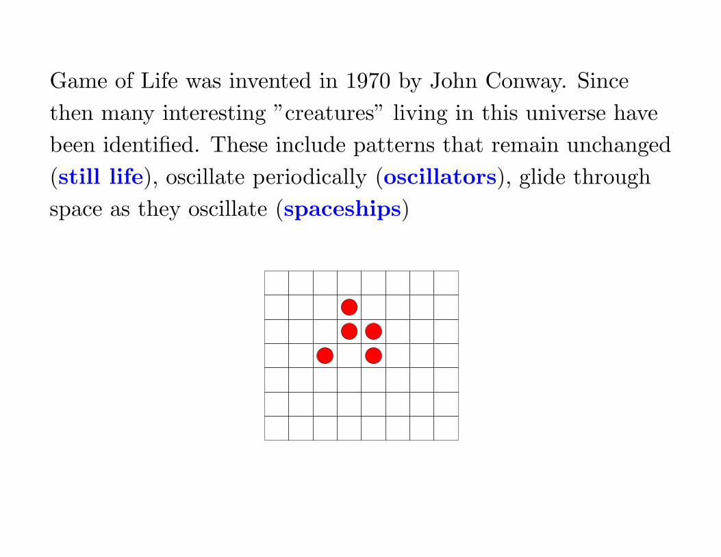
Game of Life was invented in 1970 by John Conway. Since
then many interesting ”creatures” living in this universe have
been identified. These include patterns that remain unchanged
(still life), oscillate periodically (oscillators), glide through
space as they oscillate (spaceships)
Game of Life was invented in 1970 by John Conway. Since
then many interesting ”creatures” living in this universe have
been identified. These include patterns that remain unchanged
(still life), oscillate periodically (oscillators), glide through
space as they oscillate (spaceships)
Game of Life was invented in 1970 by John Conway. Since
then many interesting ”creatures” living in this universe have
been identified. These include patterns that remain unchanged
(still life), oscillate periodically (oscillators), glide through
space as they oscillate (spaceships)
Game of Life was invented in 1970 by John Conway. Since
then many interesting ”creatures” living in this universe have
been identified. These include patterns that remain unchanged
(still life), oscillate periodically (oscillators), glide through
space as they oscillate (spaceships)
Game of Life was invented in 1970 by John Conway. Since
then many interesting ”creatures” living in this universe have
been identified. These include patterns that remain unchanged
(still life), oscillate periodically (oscillators), glide through
space as they oscillate (spaceships)
Game of Life was invented in 1970 by John Conway. Since
then many interesting ”creatures” living in this universe have
been identified. These include patterns that remain unchanged
(still life), oscillate periodically (oscillators), glide through
space as they oscillate (spaceships)
Game of Life was invented in 1970 by John Conway. Since
then many interesting ”creatures” living in this universe have
been identified. These include patterns that remain unchanged
(still life), oscillate periodically (oscillators), glide through
space as they oscillate (spaceships), emit spaceships (guns),
etc.
Using such behaviors it is possible to implement information
carrying signals and logical operations on these signals. It was
soon discovered that Game-of-Life is a universal computer:
for any given Turing machine M and input word w one can
effectively construct a start configuration c to the Game-of-Life
such that all cells eventually die if and only if M accepts w.
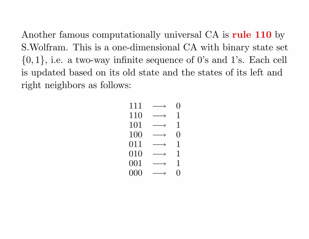
Another famous computationally universal CA is rule 110 by
S.Wolfram. This is a one-dimensional CA with binary state set
{0, 1}, i.e. a two-way infinite sequence of 0’s and 1’s. Each cell
is updated based on its old state and the states of its left and
right neighbors as follows:
111 −→ 0110 −→ 1101 −→ 1100 −→ 0011 −→ 1010 −→ 1001 −→ 1000 −→ 0
Rule 110 was proved universal by M.Cook while working for
Wolfram. Analogously to Game-of-Life, it is possible to
identify signals that transmit information, and collisions that
represent logic operations, but building a computer in the
one-dimensional space involves solving difficult issues such as
designing ways for the signals to cross each other.
One-dimensional, binary state CA that use the nearest
neighbors to determine their next state are called elementary
cellular automata. There are only 28 = 256 elementary CA,
and it is quite remarkable that one of them is computationally
universal.
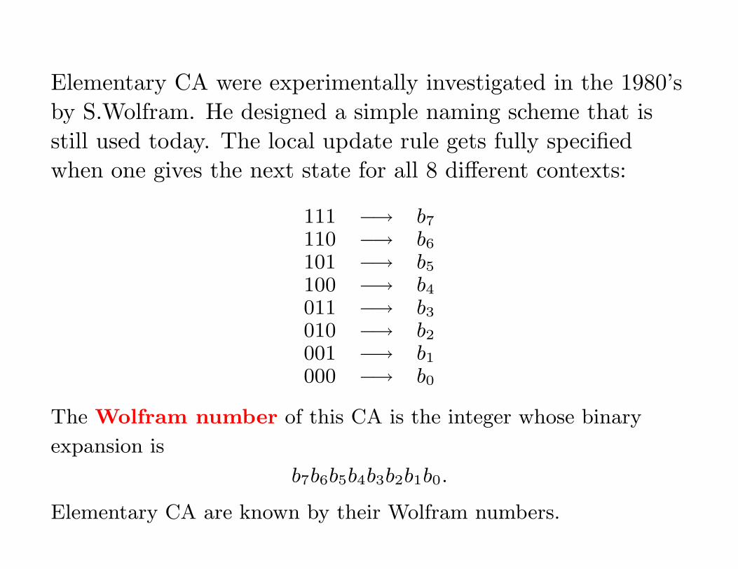
Elementary CA were experimentally investigated in the 1980’s
by S.Wolfram. He designed a simple naming scheme that is
still used today. The local update rule gets fully specified
when one gives the next state for all 8 different contexts:
111 −→ b7
110 −→ b6
101 −→ b5
100 −→ b4
011 −→ b3
010 −→ b2
001 −→ b1
000 −→ b0
The Wolfram number of this CA is the integer whose binary
expansion is
b7b6b5b4b3b2b1b0.
Elementary CA are known by their Wolfram numbers.
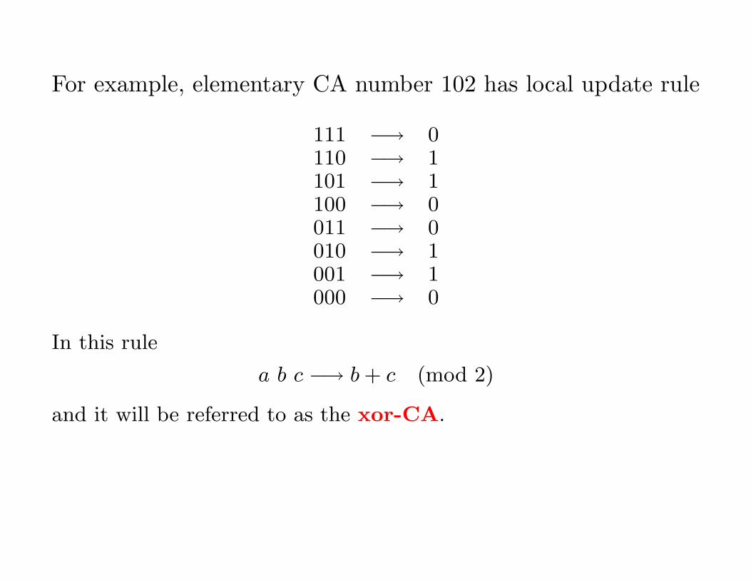
For example, elementary CA number 102 has local update rule
111 −→ 0110 −→ 1101 −→ 1100 −→ 0011 −→ 0010 −→ 1001 −→ 1000 −→ 0
In this rule
a b c −→ b + c (mod 2)
and it will be referred to as the xor-CA.
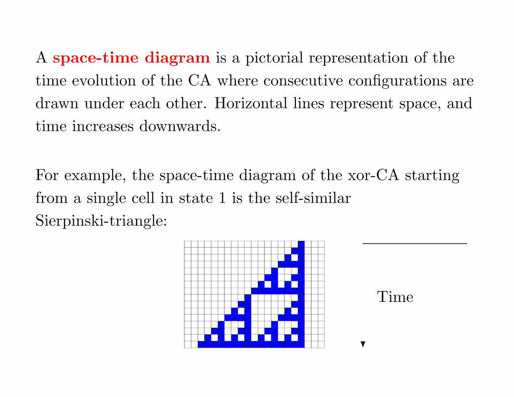
A space-time diagram is a pictorial representation of the
time evolution of the CA where consecutive configurations are
drawn under each other. Horizontal lines represent space, and
time increases downwards.
For example, the space-time diagram of the xor-CA starting
from a single cell in state 1 is the self-similar
Sierpinski-triangle:
?
Time
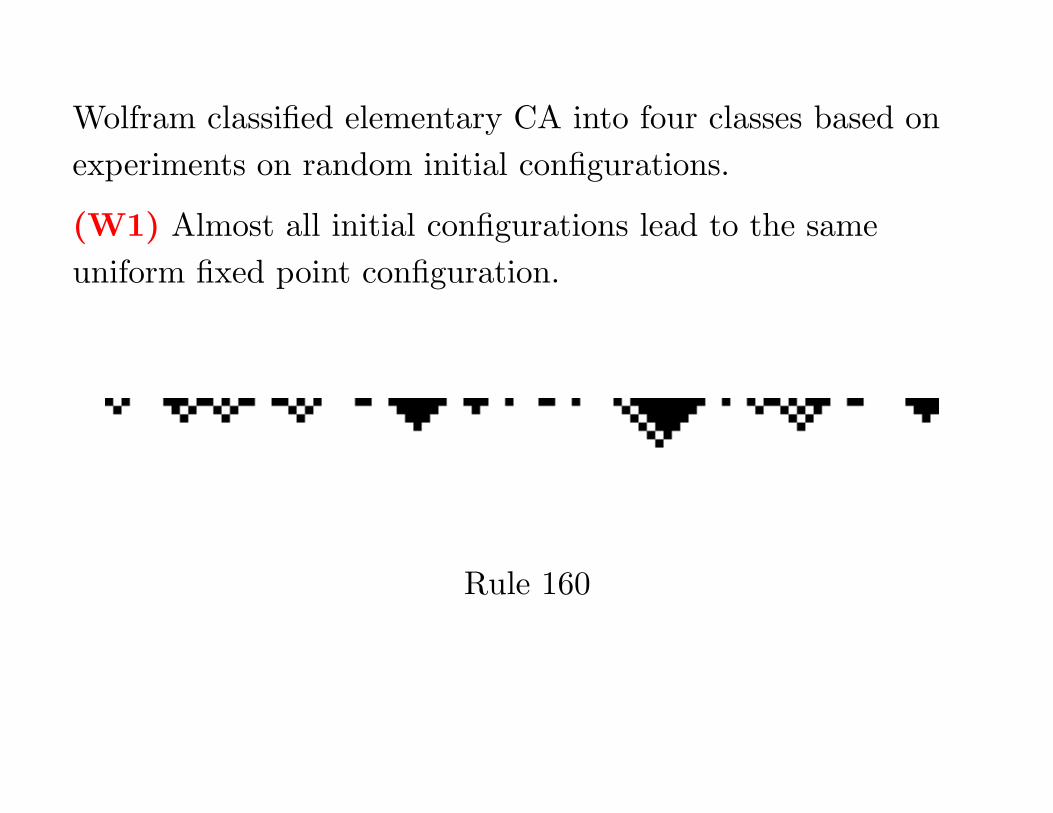
Wolfram classified elementary CA into four classes based on
experiments on random initial configurations.
(W1) Almost all initial configurations lead to the same
uniform fixed point configuration.
Rule 160
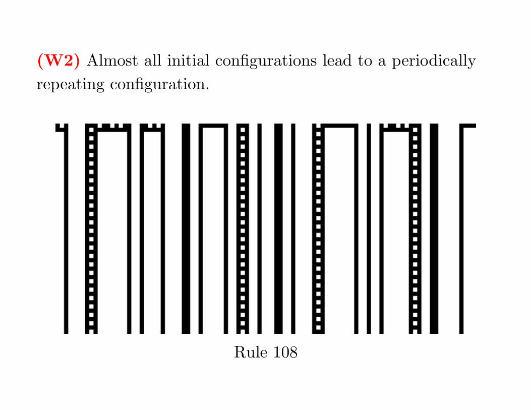
(W2) Almost all initial configurations lead to a periodically
repeating configuration.
Rule 108
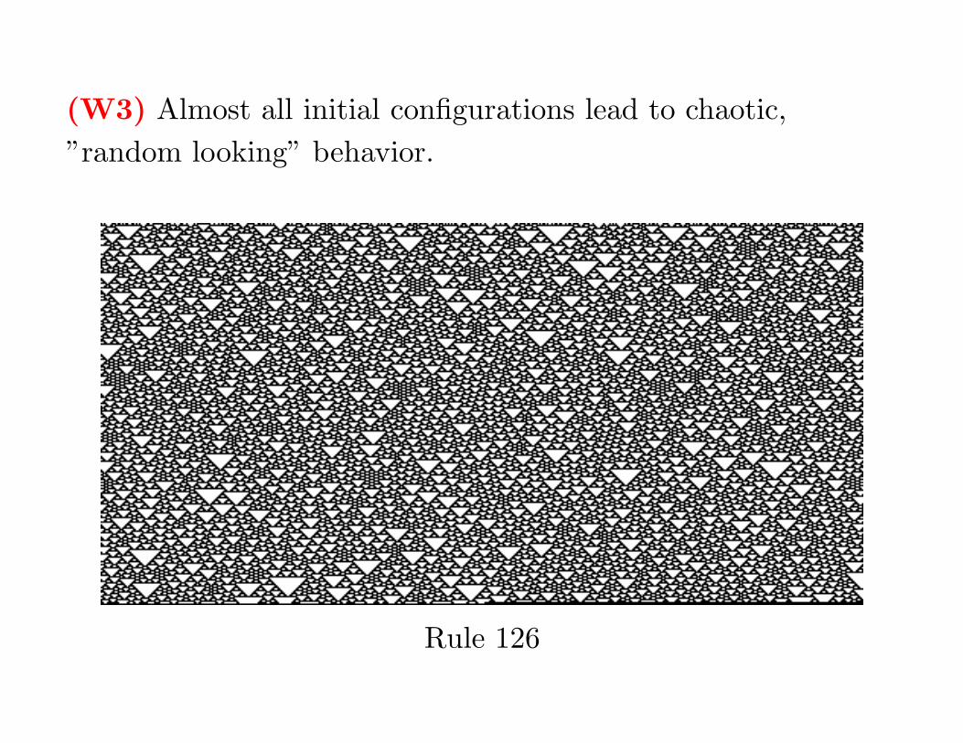
(W3) Almost all initial configurations lead to chaotic,
”random looking” behavior.
Rule 126
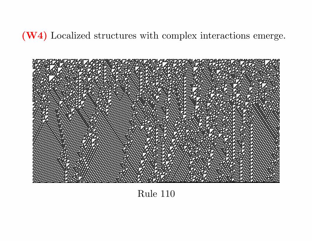
(W4) Localized structures with complex interactions emerge.
Rule 110
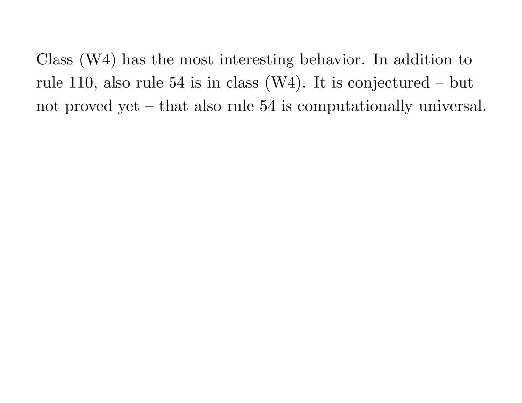
Class (W4) has the most interesting behavior. In addition to
rule 110, also rule 54 is in class (W4). It is conjectured – but
not proved yet – that also rule 54 is computationally universal.
Outline of the talk(s)
(1) Definitions (configurations, neighborhoods, cellular
automata, reversibility, injectivity, surjectivity)
Outline of the talk(s)
(1) Definitions (configurations, neighborhoods, cellular
automata, reversibility, injectivity, surjectivity)
(2) Classical results (Hedlund’s theorem, balance in
surjective CA, Garden-Of-Eden theorem)
Outline of the talk(s)
(1) Definitions (configurations, neighborhoods, cellular
automata, reversibility, injectivity, surjectivity)
(2) Classical results (Hedlund’s theorem, balance in
surjective CA, Garden-Of-Eden theorem)
(3) Reversible CA (universality, billiard ball CA)
Outline of the talk(s)
(1) Definitions (configurations, neighborhoods, cellular
automata, reversibility, injectivity, surjectivity)
(2) Classical results (Hedlund’s theorem, balance in
surjective CA, Garden-Of-Eden theorem)
(3) Reversible CA (universality, billiard ball CA)
(4) Decidability questions (Wang tiles, domino problem,
snake tiles, undecidability of nilpotency, reversibility,
surjectivity, periodicity)
(5) Dynamical systems aspects (equicontinuity
classification, limit sets)
Cellular Automata: definitions
A Cellular Automaton (CA) is an infinite lattice of finite
state machines, called cells. The cells of a d-dimensional CA
are positioned at the integer lattice points of the d-dimensional
Euclidean space, and they are addressed by the elements of Zd.
Let S be the finite state set. A configuration of the CA is a
function
c : Zd −→ S
where c(~x) is the current state of the cell ~x. The set SZd
of all
configurations is uncountably infinite.
The cells change their states synchronously at discrete time
steps. The next state of each cell depends on the current states
of the neighboring cells according to an update rule. All cells
use the same rule, and the rule is applied to all cells at the
same time.
The cells change their states synchronously at discrete time
steps. The next state of each cell depends on the current states
of the neighboring cells according to an update rule. All cells
use the same rule, and the rule is applied to all cells at the
same time.
The neighboring cells may be the nearest cells surrounding
each cell, but more general neighborhoods can be specified by
giving the relative offsets of the neighbors. Let
N = (~x1, ~x2, . . . , ~xn)
be a vector of n distinct elements of Zd. Then the neighbors
of a cell at location ~x ∈ Zd are the n cells at locations
~x + ~xi, for i = 1, 2, . . . , n.
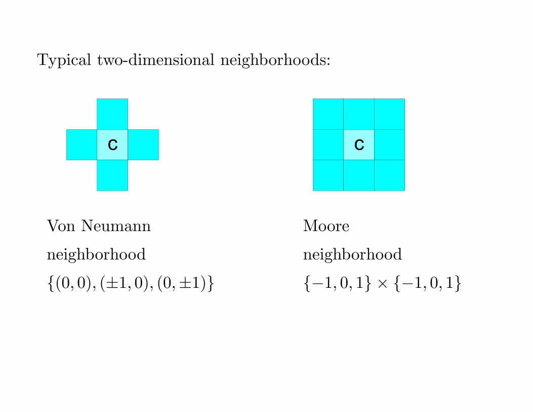
Typical two-dimensional neighborhoods:
c c
Von Neumann Moore
neighborhood neighborhood
{(0, 0), (±1, 0), (0,±1)} {−1, 0, 1} × {−1, 0, 1}
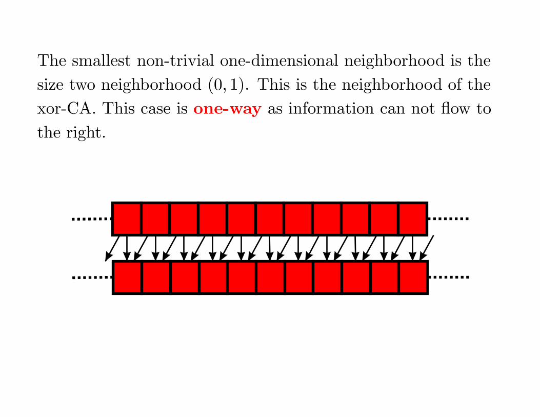
The smallest non-trivial one-dimensional neighborhood is the
size two neighborhood (0, 1). This is the neighborhood of the
xor-CA. This case is one-way as information can not flow to
the right.
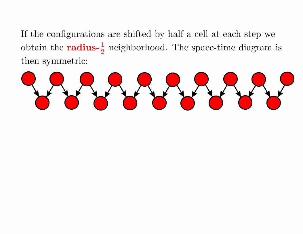
If the configurations are shifted by half a cell at each step we
obtain the radius- 12 neighborhood. The space-time diagram is
then symmetric:
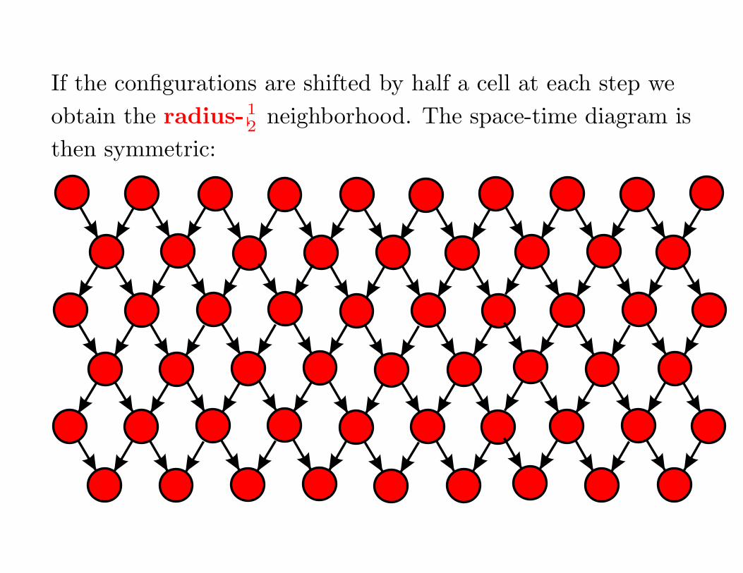
If the configurations are shifted by half a cell at each step we
obtain the radius- 12 neighborhood. The space-time diagram is
then symmetric:
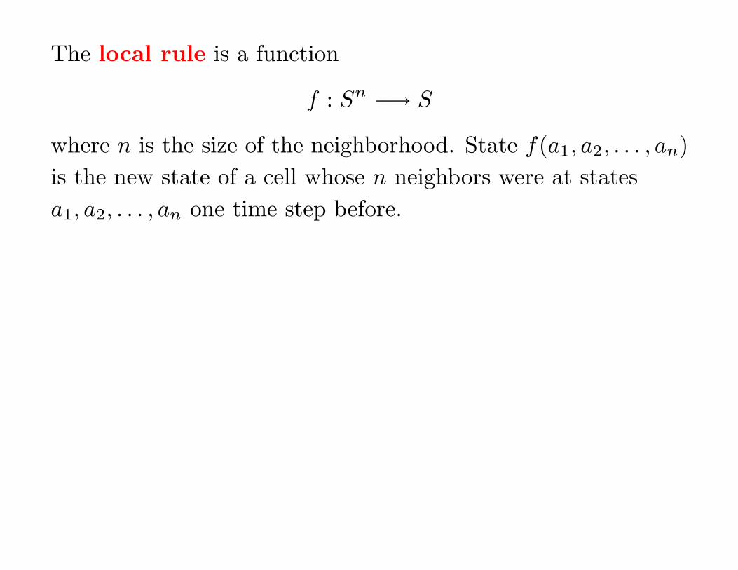
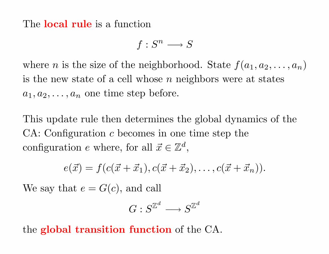
The local rule is a function
f : Sn −→ S
where n is the size of the neighborhood. State f(a1, a2, . . . , an)
is the new state of a cell whose n neighbors were at states
a1, a2, . . . , an one time step before.
The local rule is a function
f : Sn −→ S
where n is the size of the neighborhood. State f(a1, a2, . . . , an)
is the new state of a cell whose n neighbors were at states
a1, a2, . . . , an one time step before.
This update rule then determines the global dynamics of the
CA: Configuration c becomes in one time step the
configuration e where, for all ~x ∈ Zd,
e(~x) = f(c(~x + ~x1), c(~x + ~x2), . . . , c(~x + ~xn)).
We say that e = G(c), and call
G : SZd
−→ SZd
the global transition function of the CA.
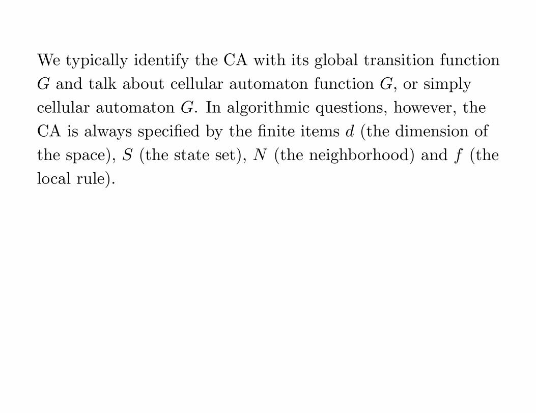
We typically identify the CA with its global transition function
G and talk about cellular automaton function G, or simply
cellular automaton G. In algorithmic questions, however, the
CA is always specified by the finite items d (the dimension of
the space), S (the state set), N (the neighborhood) and f (the
local rule).
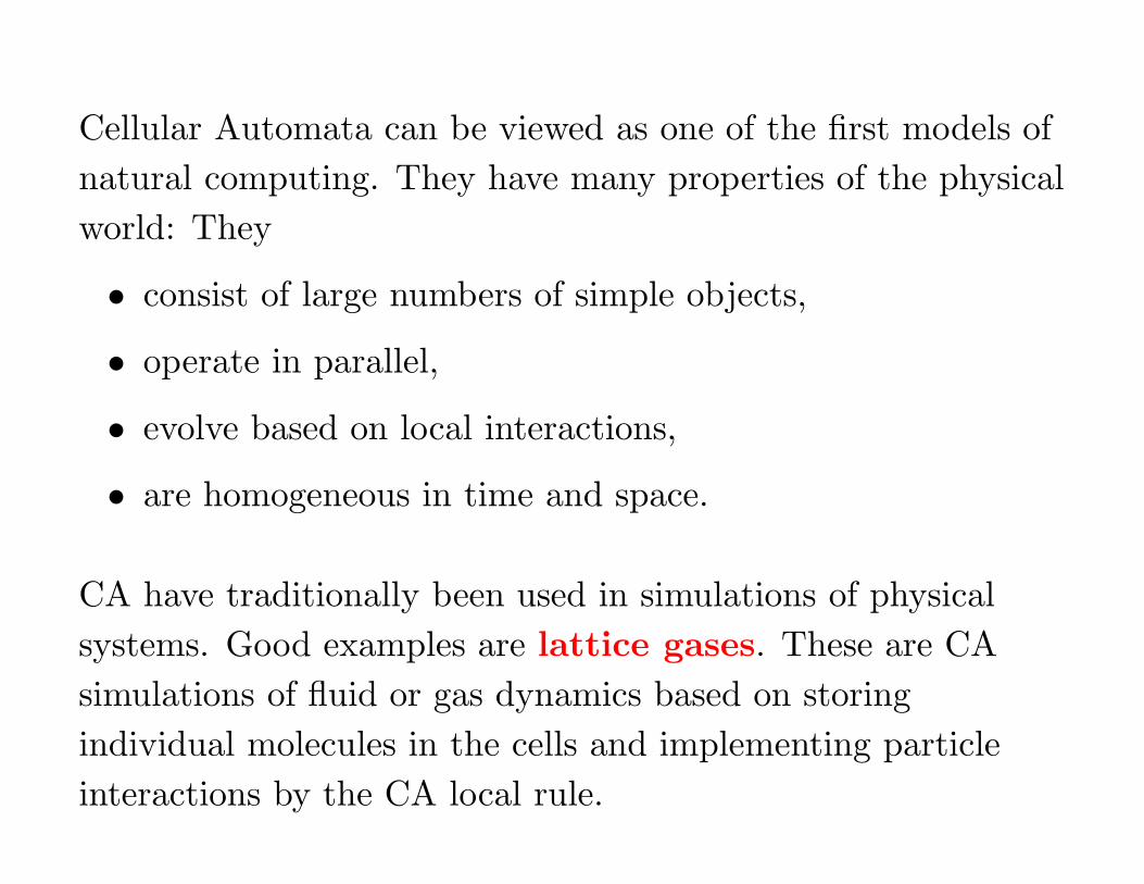
Cellular Automata can be viewed as one of the first models of
natural computing. They have many properties of the physical
world: They
• consist of large numbers of simple objects,
• operate in parallel,
• evolve based on local interactions,
• are homogeneous in time and space.
CA have traditionally been used in simulations of physical
systems. Good examples are lattice gases. These are CA
simulations of fluid or gas dynamics based on storing
individual molecules in the cells and implementing particle
interactions by the CA local rule.
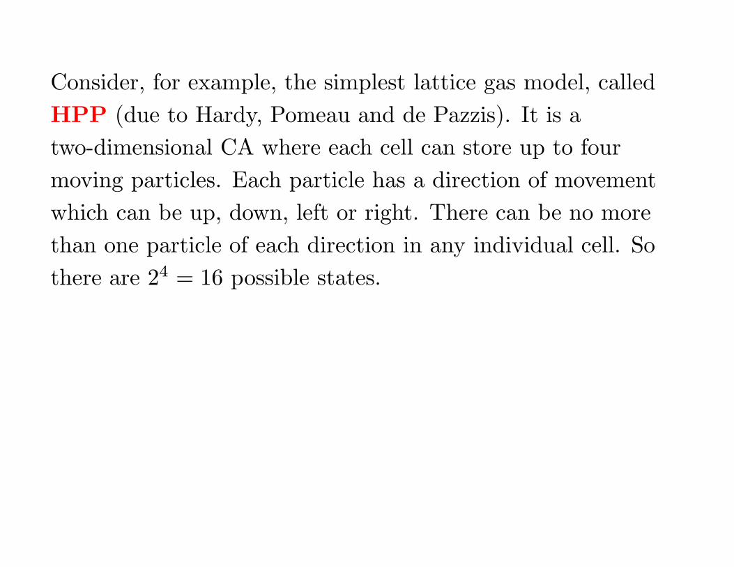
Consider, for example, the simplest lattice gas model, called
HPP (due to Hardy, Pomeau and de Pazzis). It is a
two-dimensional CA where each cell can store up to four
moving particles. Each particle has a direction of movement
which can be up, down, left or right. There can be no more
than one particle of each direction in any individual cell. So
there are 24 = 16 possible states.
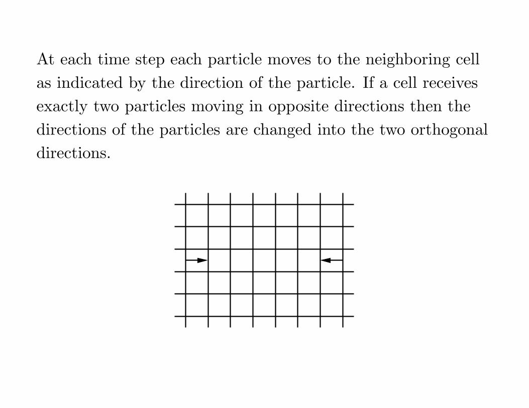
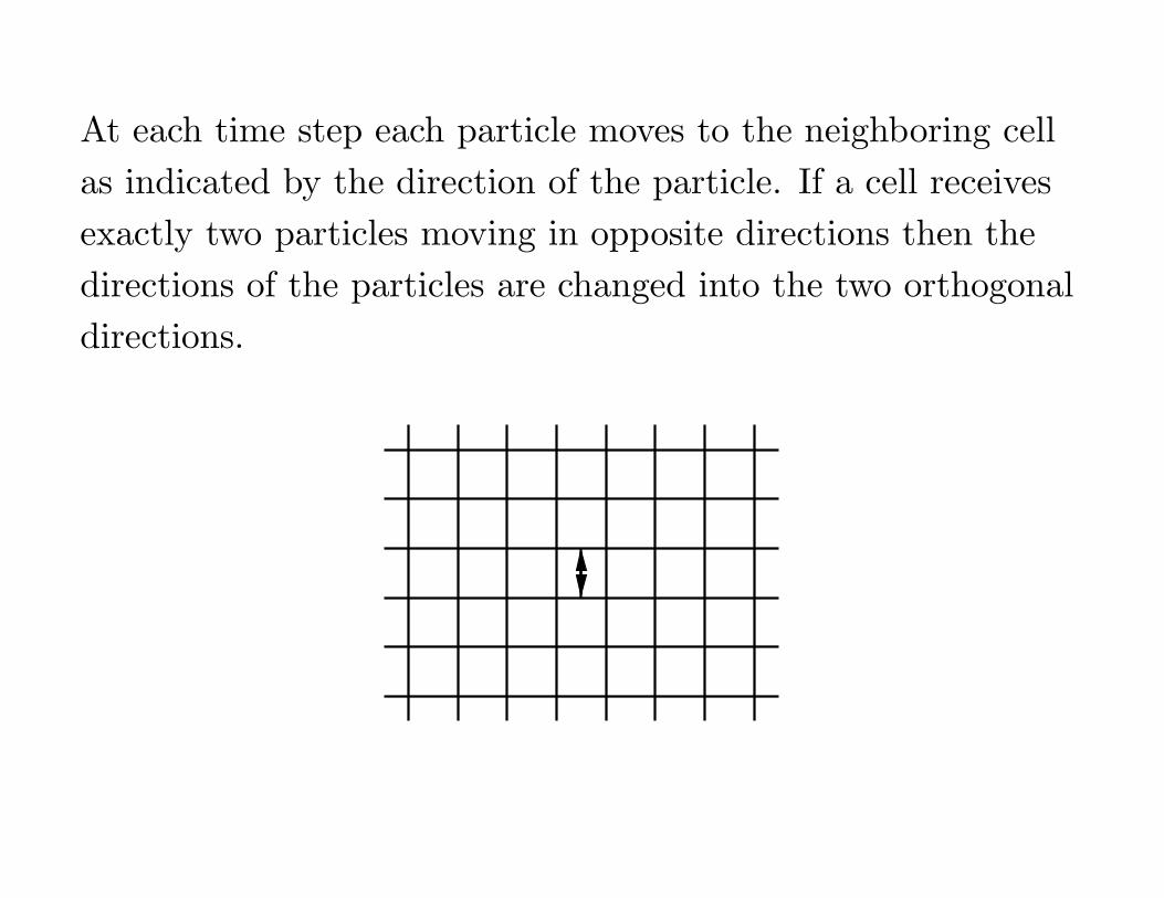
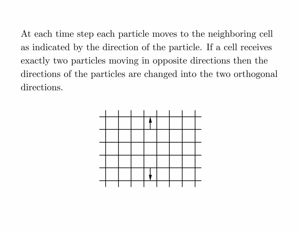
At each time step each particle moves to the neighboring cell
as indicated by the direction of the particle. If a cell receives
exactly two particles moving in opposite directions then the
directions of the particles are changed into the two orthogonal
directions.

At each time step each particle moves to the neighboring cell
as indicated by the direction of the particle. If a cell receives
exactly two particles moving in opposite directions then the
directions of the particles are changed into the two orthogonal
directions.

At each time step each particle moves to the neighboring cell
as indicated by the direction of the particle. If a cell receives
exactly two particles moving in opposite directions then the
directions of the particles are changed into the two orthogonal
directions.
At each time step each particle moves to the neighboring cell
as indicated by the direction of the particle. If a cell receives
exactly two particles moving in opposite directions then the
directions of the particles are changed into the two orthogonal
directions.

At each time step each particle moves to the neighboring cell
as indicated by the direction of the particle. If a cell receives
exactly two particles moving in opposite directions then the
directions of the particles are changed into the two orthogonal
directions.
At each time step each particle moves to the neighboring cell
as indicated by the direction of the particle. If a cell receives
exactly two particles moving in opposite directions then the
directions of the particles are changed into the two orthogonal
directions.
The local rule of HPP preserves the total number of particles
and their total momentum. These are conservation laws
that hold in the HPP automaton.
(Note, however, that HPP is not a realistic lattice gas model
as it satisfies incorrect conservation laws. For example, the
horizontal momentum is preserved on each horizontal line
individually.)
Even more interestingly, the HPP local rule fully preserves
information. There is another CA that traces back the
configurations in the reverse direction. This inverse CA
simply moves the particles to the opposite direction, and
applies the same collision rule as HPP.
HPP is an example of reversible CA (RCA), also called
invertible CA. These are CA functions G such that there is
another CA function F that is its inverse, i.e.
G ◦ F = F ◦ G = identity function.
RCA G and F are called the inverse automata of each other.
Clearly, in order to be reversible G has to be a bijective
function SZd
−→ SZd
.
A CA is called
• injective if G is one-to-one,
• surjective if G is onto,
• bijective if G is both one-to-one and onto.
Outline of the talk(s)
(1) Definitions (configurations, neighborhoods, cellular
automata, reversibility, injectivity, surjectivity)
(2) Classical results (Hedlund’s theorem, balance in
surjective CA, Garden-Of-Eden theorem)
(3) Reversible CA (universality, billiard ball CA)
(4) Decidability questions (Wang tiles, domino problem,
snake tiles, undecidability of nilpotency, reversibility,
surjectivity, periodicity)
(5) Dynamical systems aspects (equicontinuity
classification, limit sets)
Classical results (1960’s and 70’s)
It is useful to endow the set SZd
of configurations with the
Cantor topology, i.e. the topology generated by the
cylinder sets
Cyl(c,M) = {e ∈ SZd
| e(~x) = c(~x) for all ~x ∈ M}
for c ∈ SZd
and finite M ⊂ Zd. The topology is compact, and
it is induced by a metric.
All cylinder sets are clopen, i.e. closed and open. Cylinders for
fixed finite M ⊆ Zd form a finite partitioning of SZ
d
.
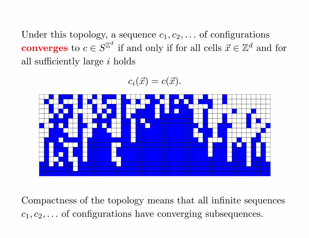
Under this topology, a sequence c1, c2, . . . of configurations
converges to c ∈ SZd
if and only if for all cells ~x ∈ Zd and for
all sufficiently large i holds
ci(~x) = c(~x).
Compactness of the topology means that all infinite sequences
c1, c2, . . . of configurations have converging subsequences.
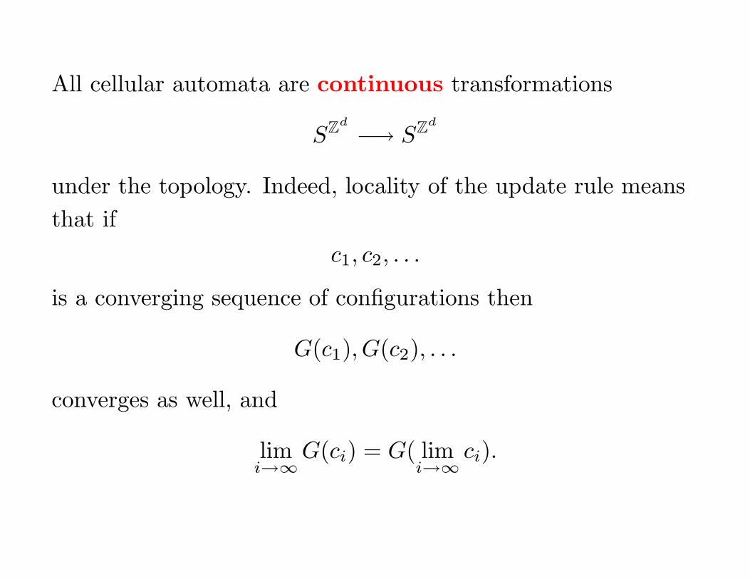
All cellular automata are continuous transformations
SZd
−→ SZd
under the topology. Indeed, locality of the update rule means
that if
c1, c2, . . .
is a converging sequence of configurations then
G(c1), G(c2), . . .
converges as well, and
limi→∞
G(ci) = G( limi→∞
ci).
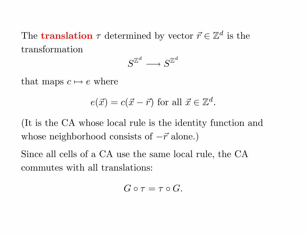
The translation τ determined by vector ~r ∈ Zd is the
transformation
SZd
−→ SZd
that maps c 7→ e where
e(~x) = c(~x − ~r) for all ~x ∈ Zd.
(It is the CA whose local rule is the identity function and
whose neighborhood consists of −~r alone.)
Since all cells of a CA use the same local rule, the CA
commutes with all translations:
G ◦ τ = τ ◦ G.
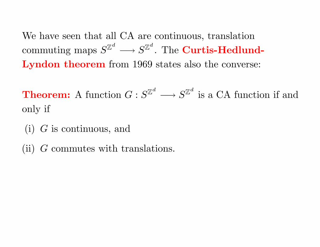
We have seen that all CA are continuous, translation
commuting maps SZd
−→ SZd
. The Curtis-Hedlund-
Lyndon theorem from 1969 states also the converse:
Theorem: A function G : SZd
−→ SZd
is a CA function if and
only if
(i) G is continuous, and
(ii) G commutes with translations.
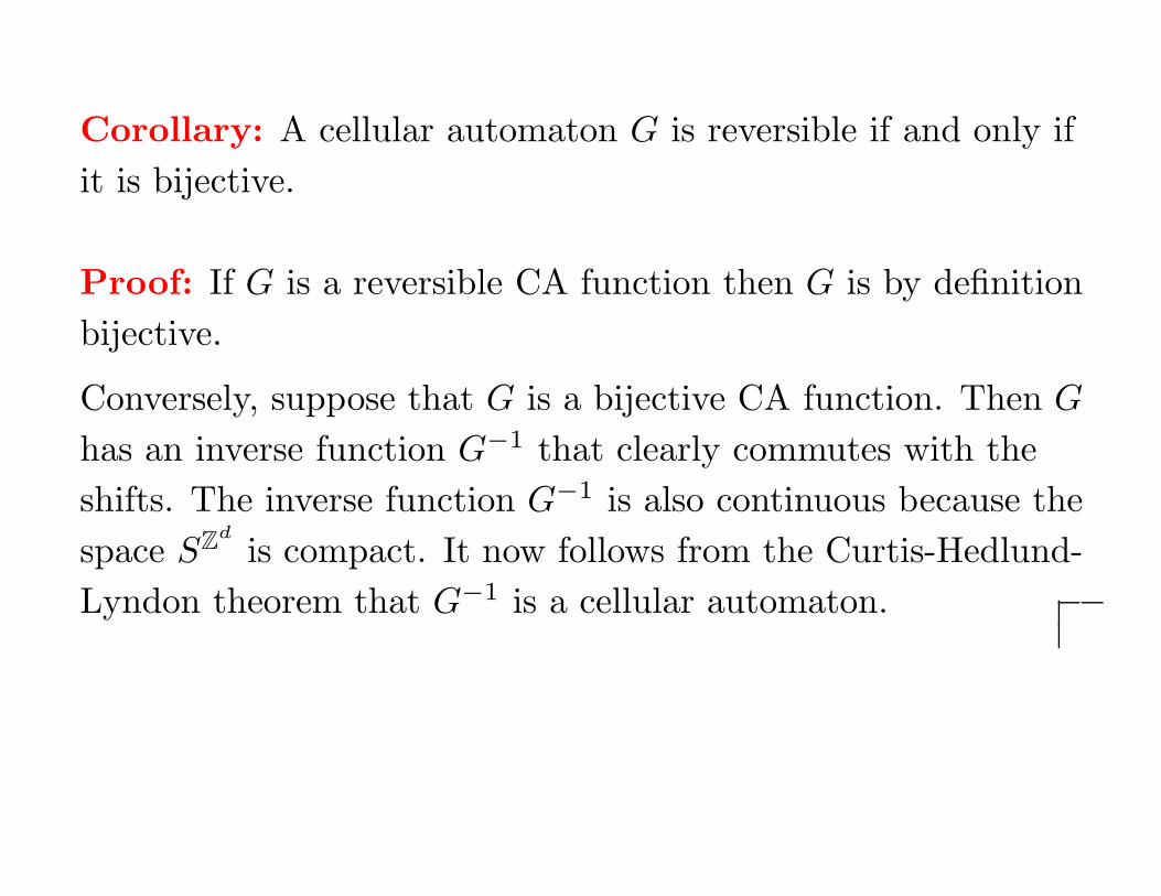
Corollary: A cellular automaton G is reversible if and only if
it is bijective.
Proof: If G is a reversible CA function then G is by definition
bijective.
Conversely, suppose that G is a bijective CA function. Then G
has an inverse function G−1 that clearly commutes with the
shifts. The inverse function G−1 is also continuous because the
space SZd
is compact. It now follows from the Curtis-Hedlund-
Lyndon theorem that G−1 is a cellular automaton.
The point of the corollary is that in bijective CA each cell can
determine its previous state by looking at the current states in
some bounded neighborhood around them.
Configurations that do not have a pre-image are called
Garden-Of-Eden -configurations. A CA has GOE
configurations if and only if it is non-surjective.
A finite pattern consists of a finite domain M ⊆ Zd and an
assignment
p : M −→ S
of states. Configuration c contains the pattern if
τ(c)|M = p
for some translation τ .
Finite pattern is called an orphan for CA G if every
configuration containing the pattern is a GOE.
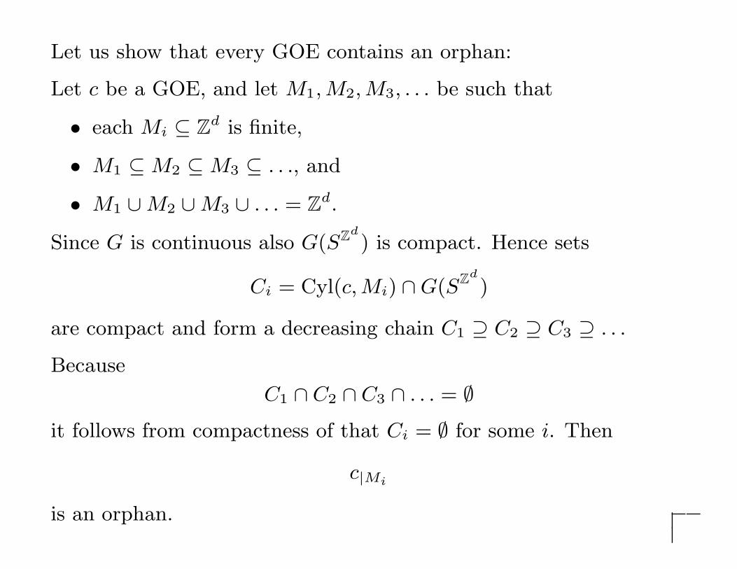
Let us show that every GOE contains an orphan:
Let c be a GOE, and let M1, M2, M3, . . . be such that
• each Mi ⊆ Zd is finite,
• M1 ⊆ M2 ⊆ M3 ⊆ . . ., and
• M1 ∪ M2 ∪ M3 ∪ . . . = Zd.
Let us show that every GOE contains an orphan:
Let c be a GOE, and let M1, M2, M3, . . . be such that
• each Mi ⊆ Zd is finite,
• M1 ⊆ M2 ⊆ M3 ⊆ . . ., and
• M1 ∪ M2 ∪ M3 ∪ . . . = Zd.
Since G is continuous also G(SZd
) is compact. Hence sets
Ci = Cyl(c, Mi) ∩ G(SZd
)
are compact and form a decreasing chain C1 ⊇ C2 ⊇ C3 ⊇ . . .
Because
C1 ∩ C2 ∩ C3 ∩ . . . = ∅
it follows from compactness of that Ci = ∅ for some i. Then
c|Mi
is an orphan.
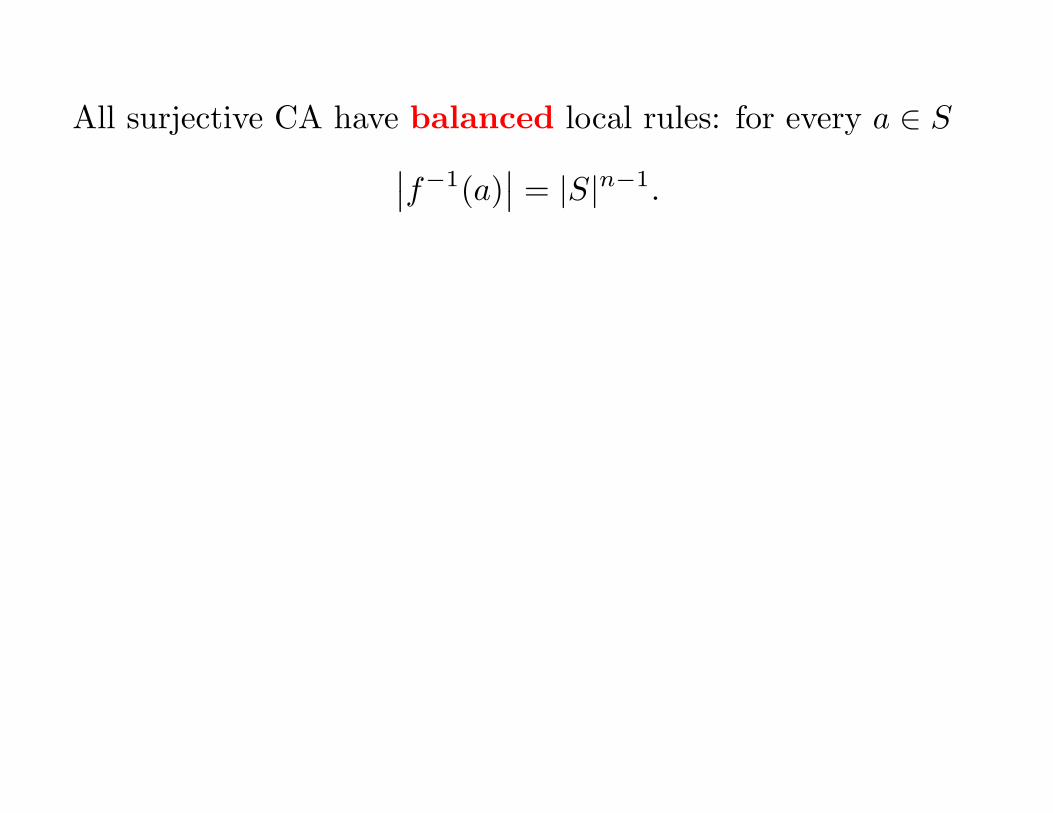
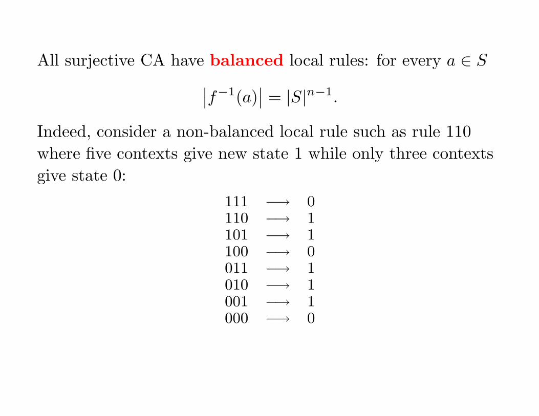
All surjective CA have balanced local rules: for every a ∈ S
∣
∣f−1(a)∣
∣ = |S|n−1.
All surjective CA have balanced local rules: for every a ∈ S
∣
∣f−1(a)∣
∣ = |S|n−1.
Indeed, consider a non-balanced local rule such as rule 110
where five contexts give new state 1 while only three contexts
give state 0:
111 −→ 0110 −→ 1101 −→ 1100 −→ 0011 −→ 1010 −→ 1001 −→ 1000 −→ 0
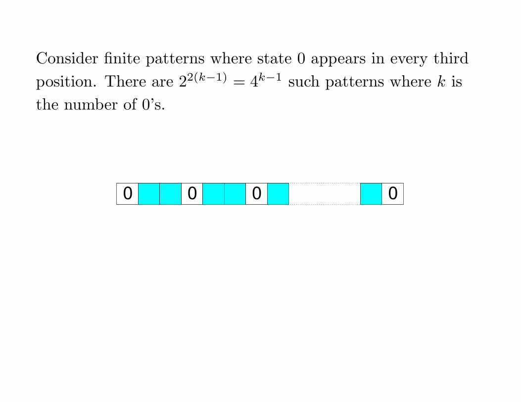
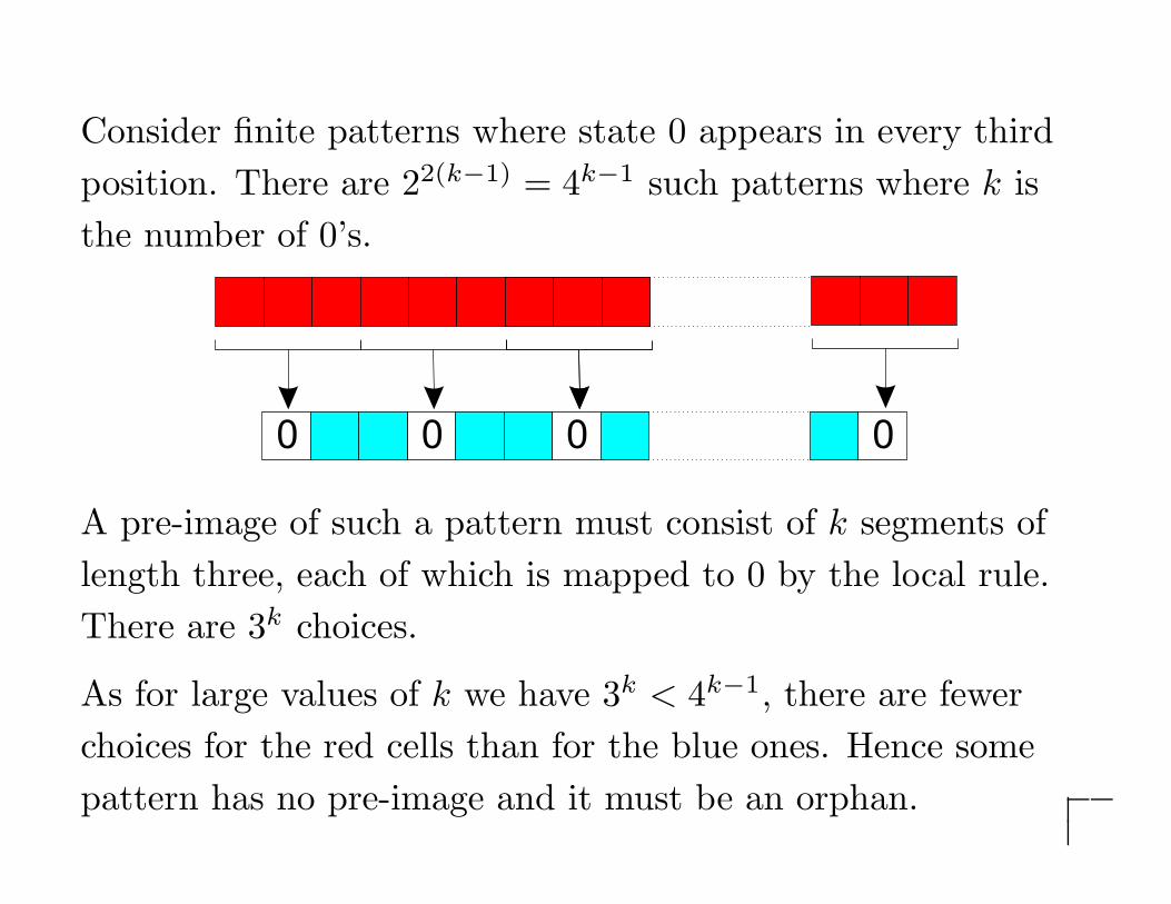
Consider finite patterns where state 0 appears in every third
position. There are 22(k−1) = 4k−1 such patterns where k is
the number of 0’s.
0 0 0 0
Consider finite patterns where state 0 appears in every third
position. There are 22(k−1) = 4k−1 such patterns where k is
the number of 0’s.
0 0 0 0
A pre-image of such a pattern must consist of k segments of
length three, each of which is mapped to 0 by the local rule.
There are 3k choices.
As for large values of k we have 3k < 4k−1, there are fewer
choices for the red cells than for the blue ones. Hence some
pattern has no pre-image and it must be an orphan.
One can also verify directly that pattern
01010
is an orphan of rule 110. It is the shortest orphan.
One can also verify directly that pattern
01010
is an orphan of rule 110. It is the shortest orphan.
Balance of the local rule is not sufficient for surjectivity. For
example, the majority CA (Wolfram number 232) is a
counter example. The local rule
f(a, b, c) = 1 if and only if a + b + c ≥ 2
is clearly balanced, but 01001 is an orphan.
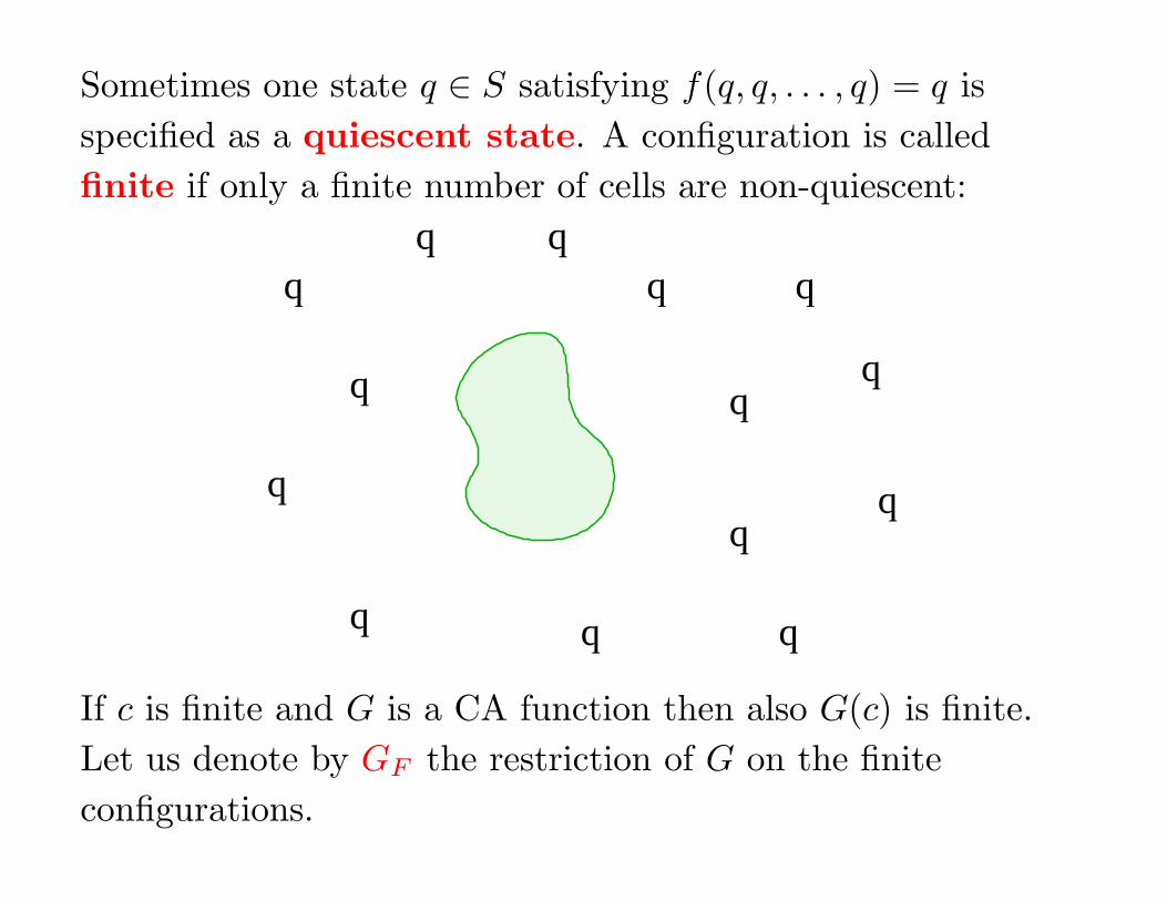
Sometimes one state q ∈ S satisfying f(q, q, . . . , q) = q is
specified as a quiescent state. A configuration is called
finite if only a finite number of cells are non-quiescent:
q
q
q q
q
q
q
q
q
q
If c is finite and G is a CA function then also G(c) is finite.
Let us denote by GF the restriction of G on the finite
configurations.
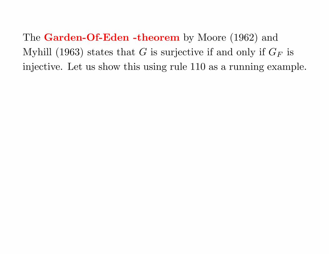
The Garden-Of-Eden -theorem by Moore (1962) and
Myhill (1963) states that G is surjective if and only if GF is
injective. Let us show this using rule 110 as a running example.
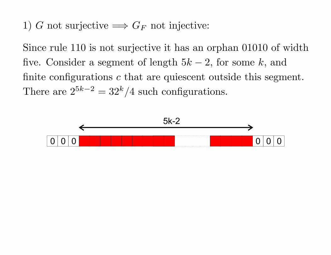
1) G not surjective =⇒ GF not injective:
Since rule 110 is not surjective it has an orphan 01010 of width
five. Consider a segment of length 5k − 2, for some k, and
finite configurations c that are quiescent outside this segment.
There are 25k−2 = 32k/4 such configurations.
0 0 0 00 0
5k-2
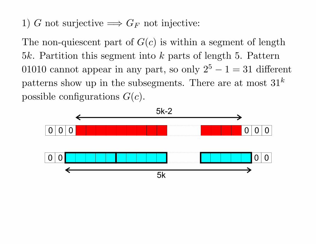
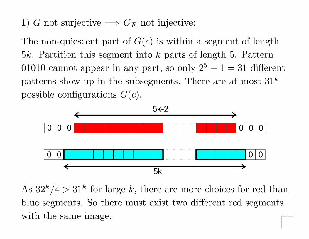
1) G not surjective =⇒ GF not injective:
The non-quiescent part of G(c) is within a segment of length
5k. Partition this segment into k parts of length 5. Pattern
01010 cannot appear in any part, so only 25 − 1 = 31 different
patterns show up in the subsegments. There are at most 31k
possible configurations G(c).
0 0 0 00 0
00 0 0
5k-2
5k
As 32k/4 > 31k for large k, there are more choices for red than
blue segments. So there must exist two different red segments
with the same image.
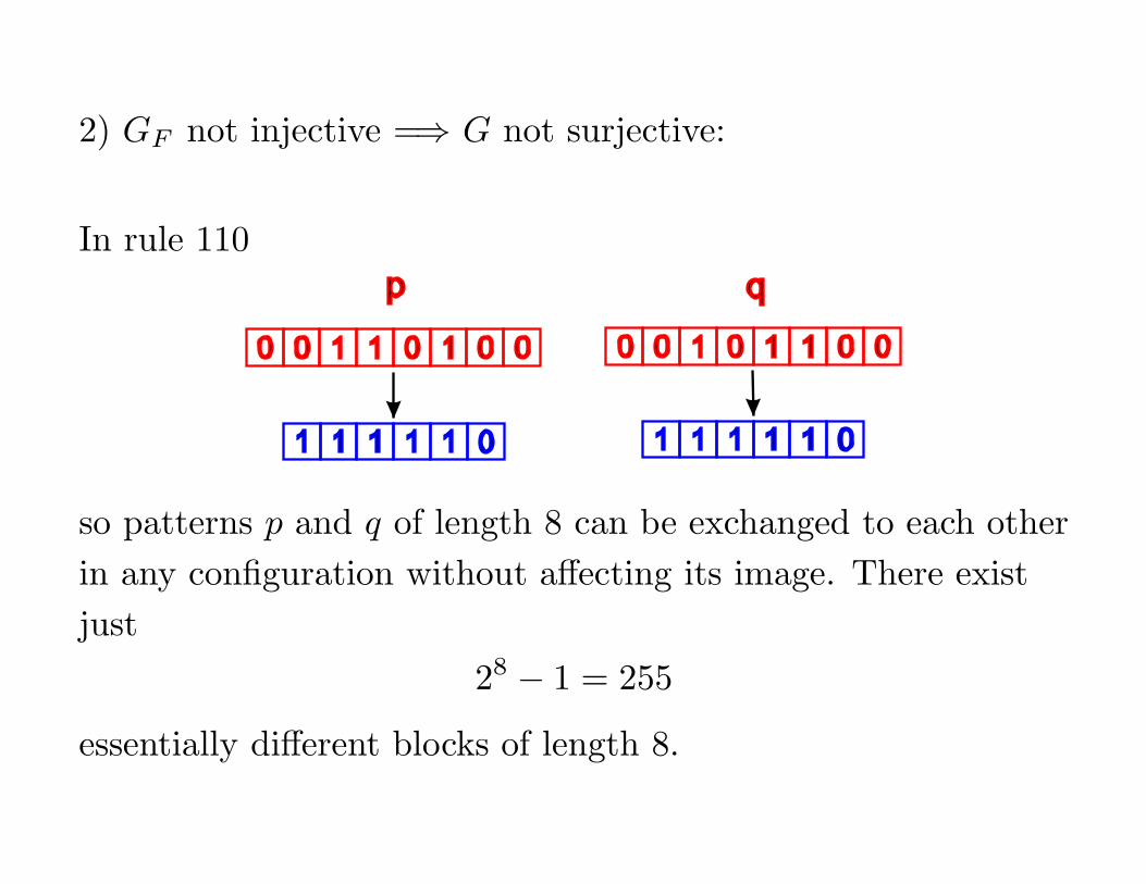
2) GF not injective =⇒ G not surjective:
In rule 110
0 10 1 0 1 0 0 0 10 0 1 1 0 0
11 1 1 1 0 11 1 1 1 0
p q
so patterns p and q of length 8 can be exchanged to each other
in any configuration without affecting its image. There exist
just
28 − 1 = 255
essentially different blocks of length 8.
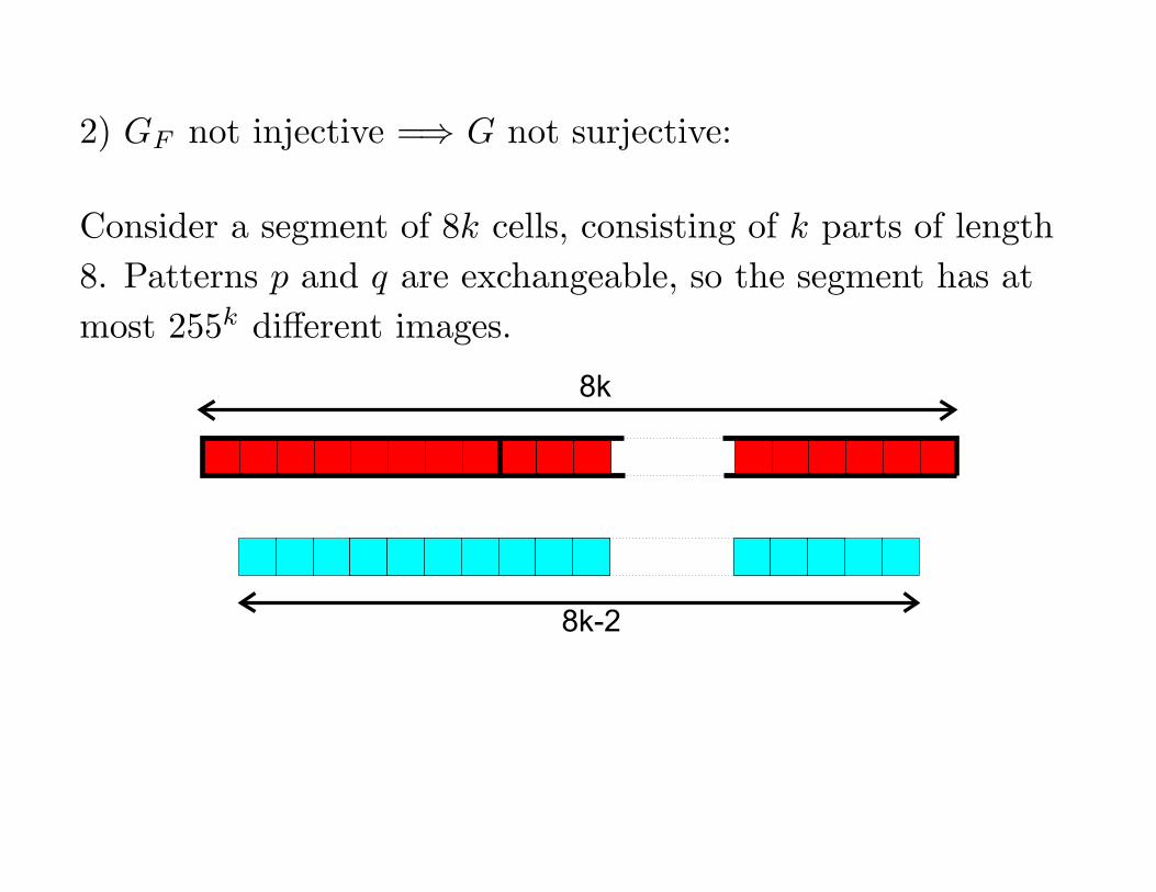
2) GF not injective =⇒ G not surjective:
Consider a segment of 8k cells, consisting of k parts of length
8. Patterns p and q are exchangeable, so the segment has at
most 255k different images.
8k
8k-2
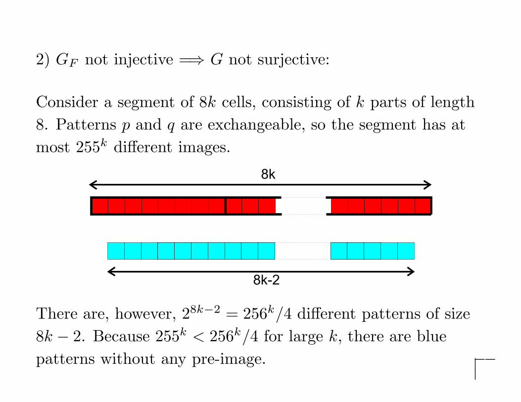
2) GF not injective =⇒ G not surjective:
Consider a segment of 8k cells, consisting of k parts of length
8. Patterns p and q are exchangeable, so the segment has at
most 255k different images.
8k
8k-2
There are, however, 28k−2 = 256k/4 different patterns of size
8k − 2. Because 255k < 256k/4 for large k, there are blue
patterns without any pre-image.
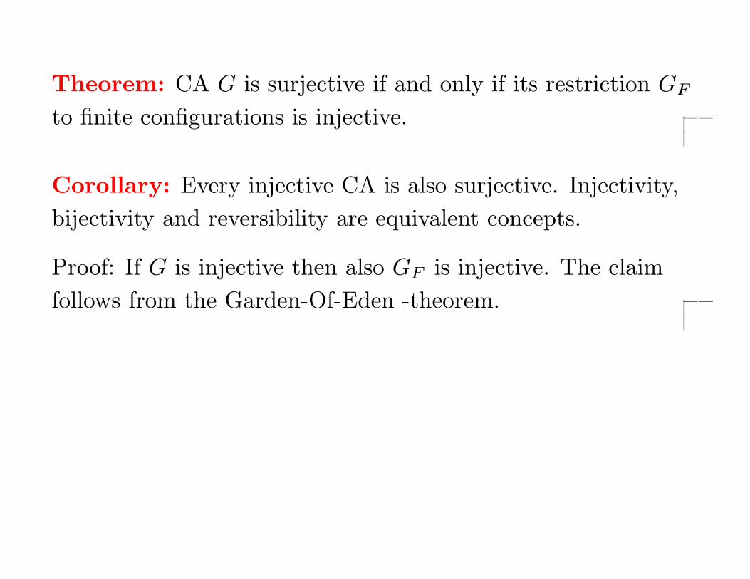
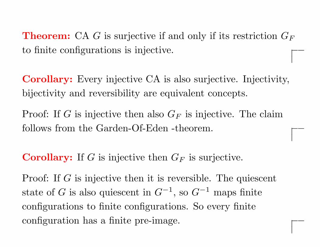
Theorem: CA G is surjective if and only if its restriction GF
to finite configurations is injective.
Theorem: CA G is surjective if and only if its restriction GF
to finite configurations is injective.
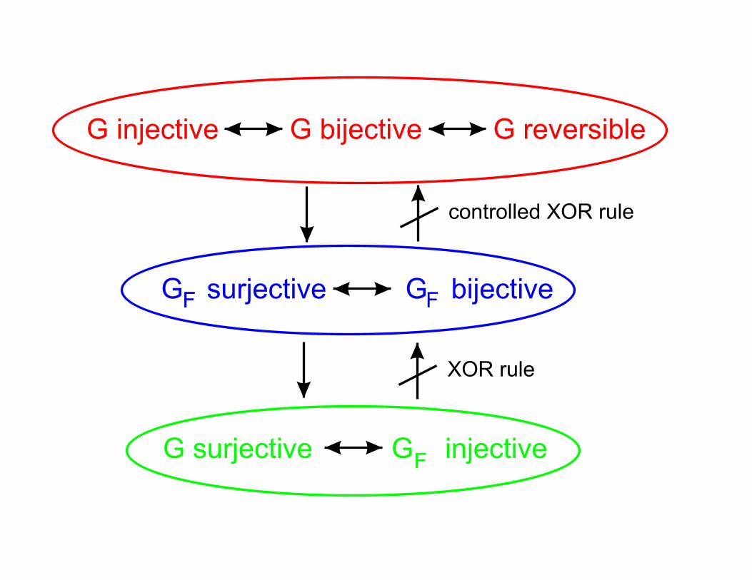
Corollary: Every injective CA is also surjective. Injectivity,
bijectivity and reversibility are equivalent concepts.
Proof: If G is injective then also GF is injective. The claim
follows from the Garden-Of-Eden -theorem.
Theorem: CA G is surjective if and only if its restriction GF
to finite configurations is injective.
Corollary: Every injective CA is also surjective. Injectivity,
bijectivity and reversibility are equivalent concepts.
Proof: If G is injective then also GF is injective. The claim
follows from the Garden-Of-Eden -theorem.
Corollary: If G is injective then GF is surjective.
Proof: If G is injective then it is reversible. The quiescent
state of G is also quiescent in G−1, so G−1 maps finite
configurations to finite configurations. So every finite
configuration has a finite pre-image.
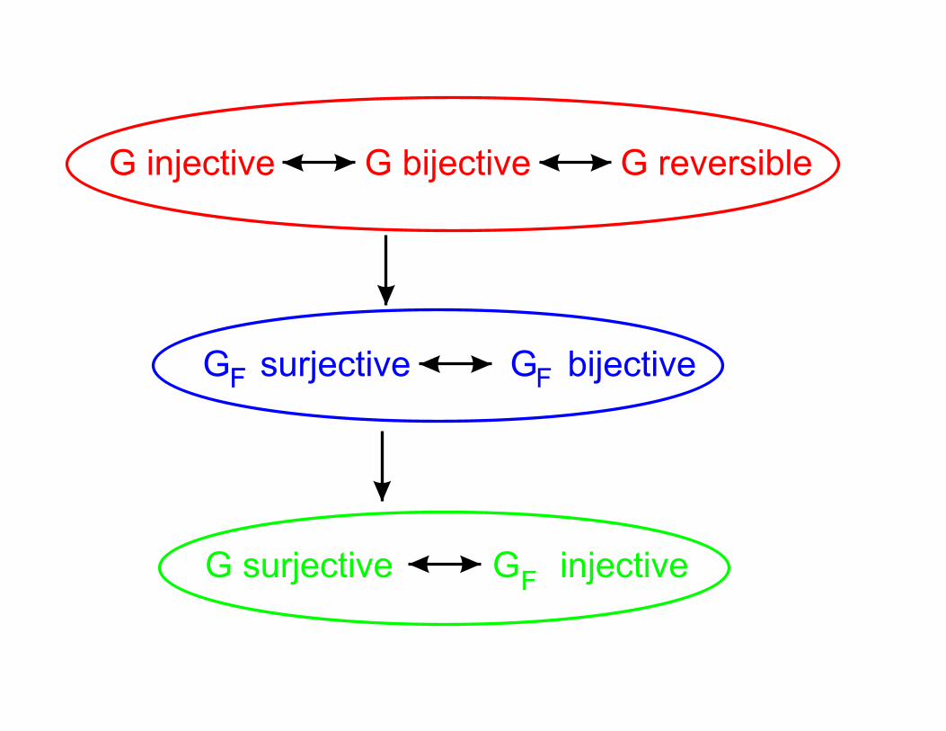
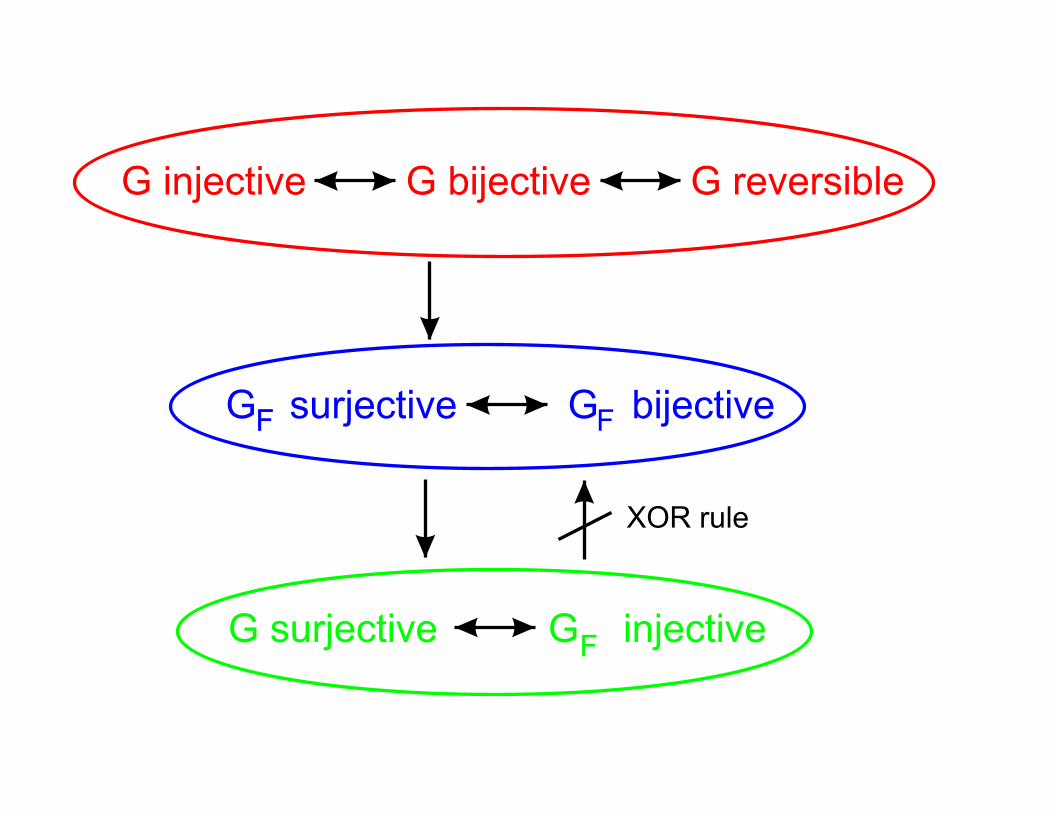
G injective G bijective G reversible
G surjective G bijective
G surjective G injective
F
F
F F

G injective G bijective G reversible
G surjective G bijective
G surjective G injective
F
F
F F
XOR rule
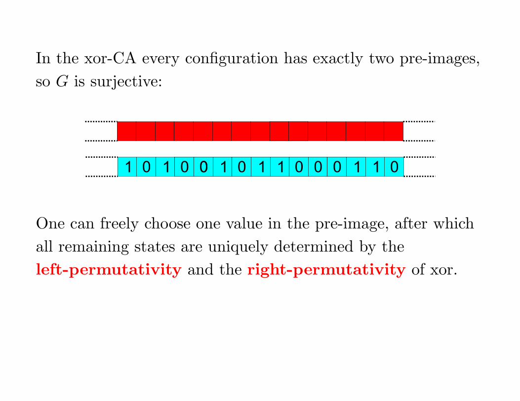
In the xor-CA every configuration has exactly two pre-images,
so G is surjective:
0 0000 0 0 0 01 1 1 1 1 1 1
One can freely choose one value in the pre-image, after which
all remaining states are uniquely determined by the
left-permutativity and the right-permutativity of xor.

In the xor-CA every configuration has exactly two pre-images,
so G is surjective:
0 0000 0 0 0 01 1 1 1 1 1 1
0
One can freely choose one value in the pre-image, after which
all remaining states are uniquely determined by the
left-permutativity and the right-permutativity of xor.

In the xor-CA every configuration has exactly two pre-images,
so G is surjective:
0 0000 0 0 0 01 1 1 1 1 1 1
0 01
One can freely choose one value in the pre-image, after which
all remaining states are uniquely determined by the
left-permutativity and the right-permutativity of xor.

In the xor-CA every configuration has exactly two pre-images,
so G is surjective:
0 0000 0 0 0 01 1 1 1 1 1 1
0 01 00 0 0 0 1
One can freely choose one value in the pre-image, after which
all remaining states are uniquely determined by the
left-permutativity and the right-permutativity of xor.

In the xor-CA every configuration has exactly two pre-images,
so G is surjective:
0 0000 0 0 0 01 1 1 1 1 1 1
0 01 00 0 0 0 10
One can freely choose one value in the pre-image, after which
all remaining states are uniquely determined by the
left-permutativity and the right-permutativity of xor.

In the xor-CA every configuration has exactly two pre-images,
so G is surjective:
0 0000 0 0 0 01 1 1 1 1 1 1
0 01 00 0 0 0 10111001
One can freely choose one value in the pre-image, after which
all remaining states are uniquely determined by the
left-permutativity and the right-permutativity of xor.
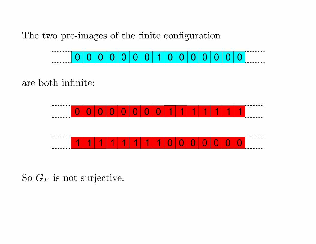
The two pre-images of the finite configuration
0 000 0 0 0 01 0 00000 0
are both infinite:
0 01 1000 1 1 1 1 10000
01 1 0001 1 1 1 1 000001
So GF is not surjective.
G injective G bijective G reversible
G surjective G bijective
G surjective G injective
F
F
F F
XOR rule

G injective G bijective G reversible
G surjective G bijective
G surjective G injective
F
F
F F
XOR rule
controlled XOR rule
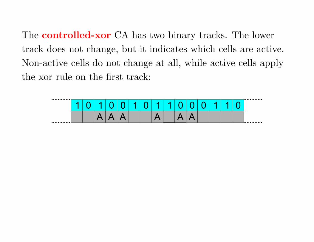
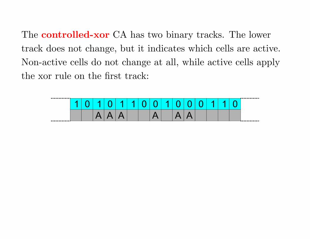
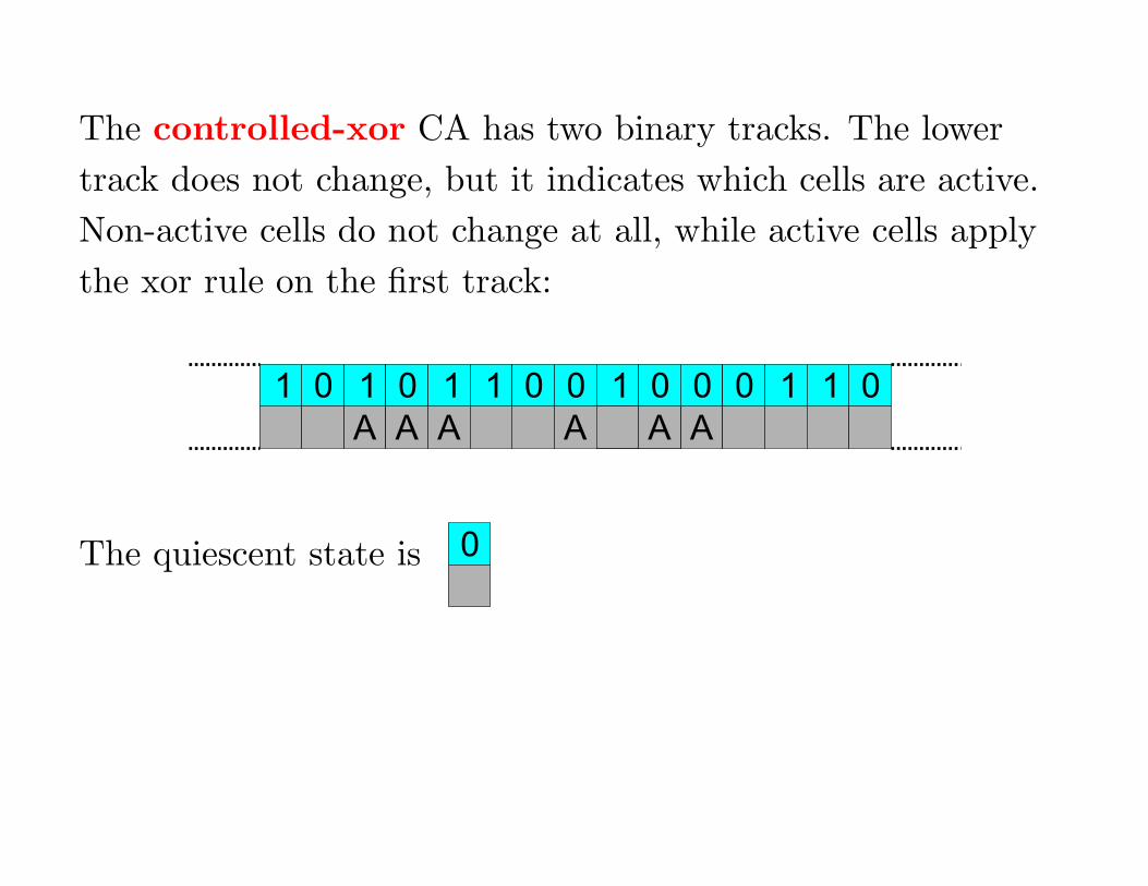
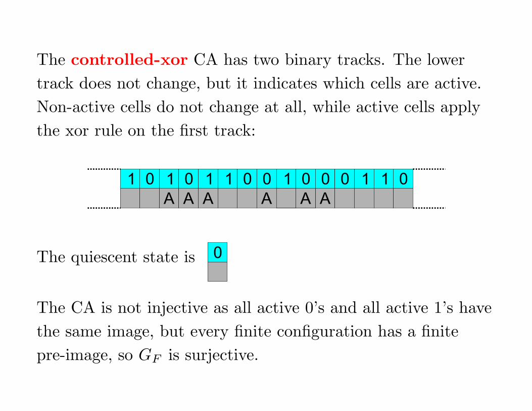
The controlled-xor CA has two binary tracks. The lower
track does not change, but it indicates which cells are active.
Non-active cells do not change at all, while active cells apply
the xor rule on the first track:
0 0000 0 0 0 01 1 1 1 1 1 1
0A A A A A A
The controlled-xor CA has two binary tracks. The lower
track does not change, but it indicates which cells are active.
Non-active cells do not change at all, while active cells apply
the xor rule on the first track:
0 00 0 0 0 01 1 1 1 1 1
0A A A A A A
1 0
The controlled-xor CA has two binary tracks. The lower
track does not change, but it indicates which cells are active.
Non-active cells do not change at all, while active cells apply
the xor rule on the first track:
0 00 0 0 0 01 1 1 1 1 1
0A A A A A A
1 0
The quiescent state is 0
The controlled-xor CA has two binary tracks. The lower
track does not change, but it indicates which cells are active.
Non-active cells do not change at all, while active cells apply
the xor rule on the first track:
0 00 0 0 0 01 1 1 1 1 1
0A A A A A A
1 0
The quiescent state is 0
The CA is not injective as all active 0’s and all active 1’s have
the same image, but every finite configuration has a finite
pre-image, so GF is surjective.
G injective G bijective G reversible
G surjective G bijective
G surjective G injective
F
F
F F
XOR rule
controlled XOR rule
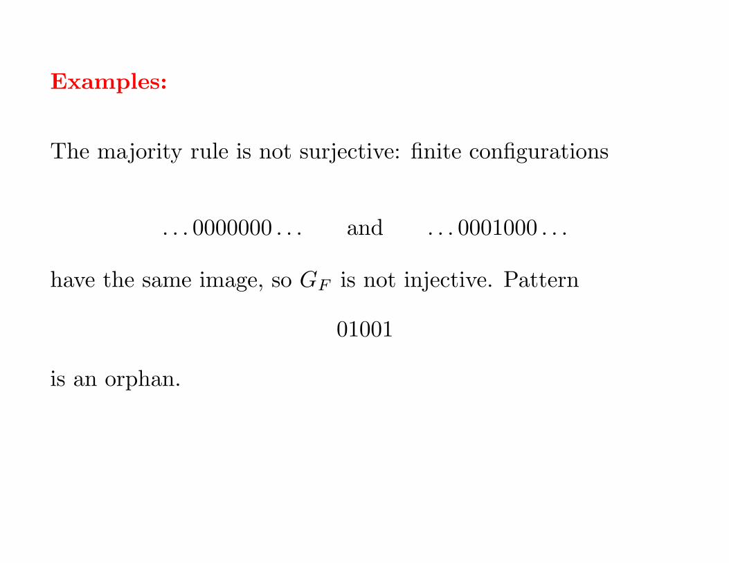
Examples:
The majority rule is not surjective: finite configurations
. . . 0000000 . . . and . . . 0001000 . . .
have the same image, so GF is not injective. Pattern
01001
is an orphan.
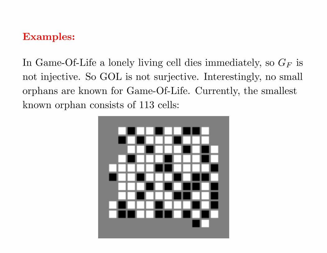
Examples:
In Game-Of-Life a lonely living cell dies immediately, so GF is
not injective. So GOL is not surjective. Interestingly, no small
orphans are known for Game-Of-Life. Currently, the smallest
known orphan consists of 113 cells:
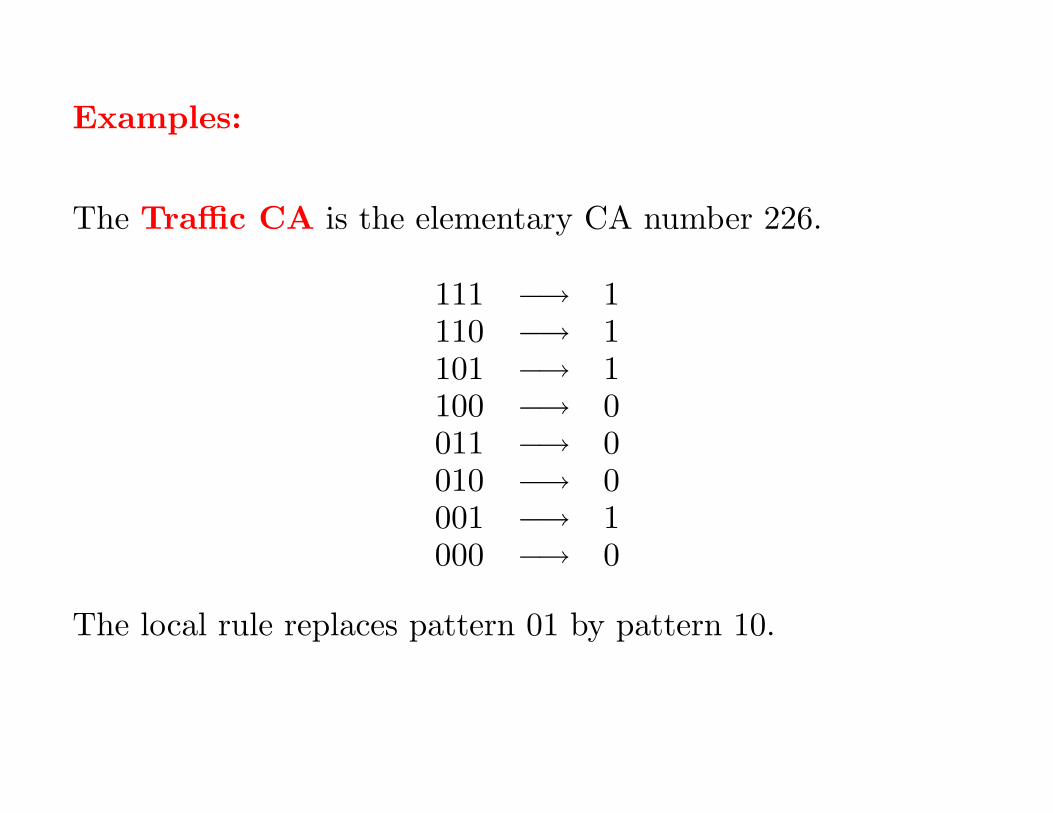
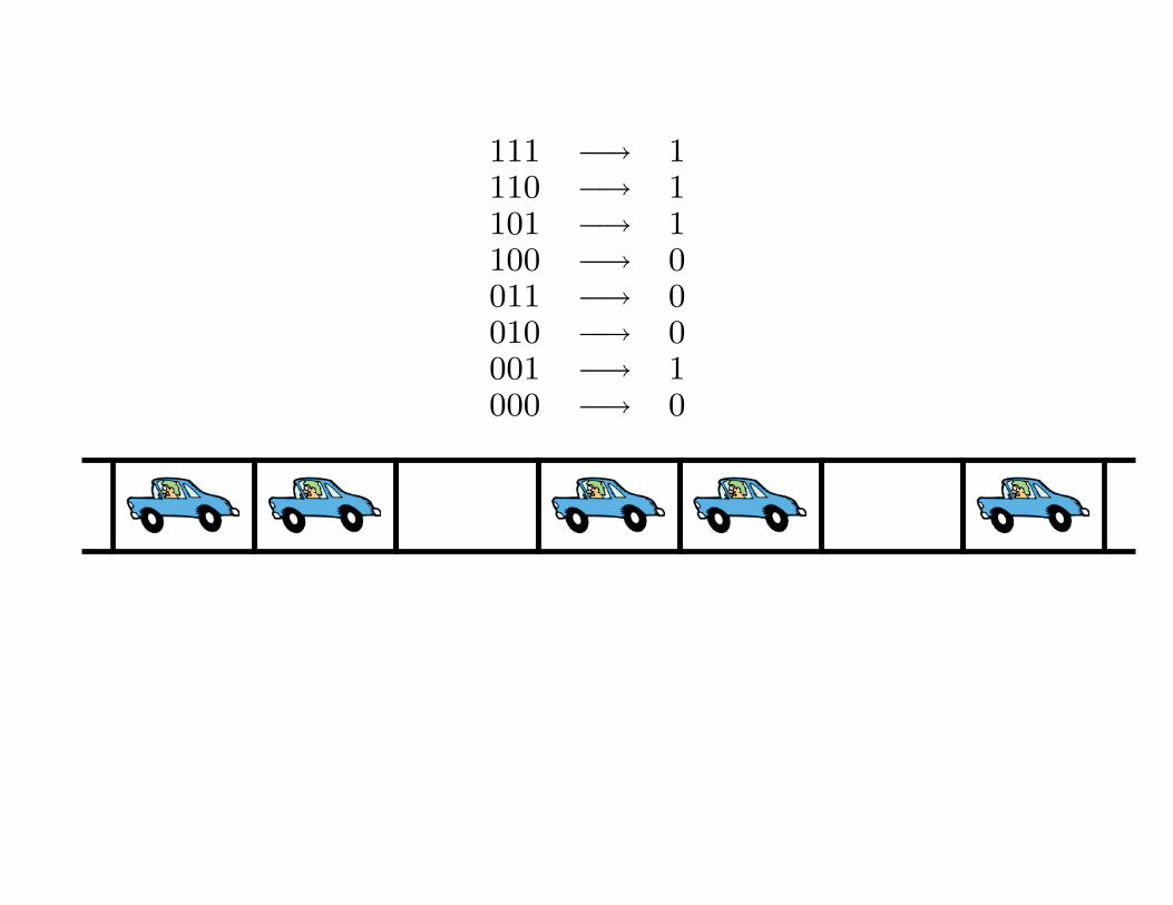
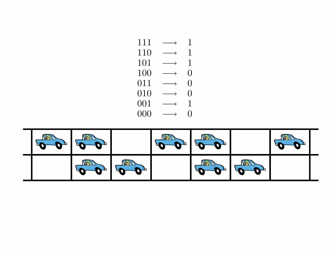
Examples:
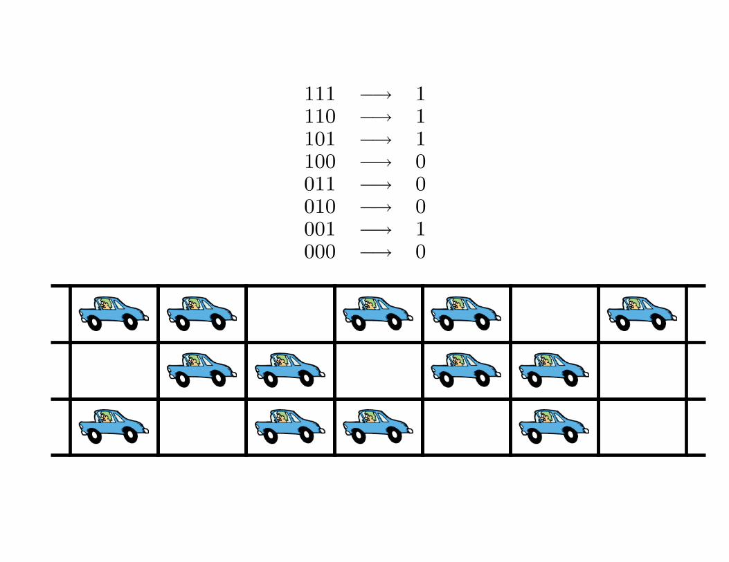
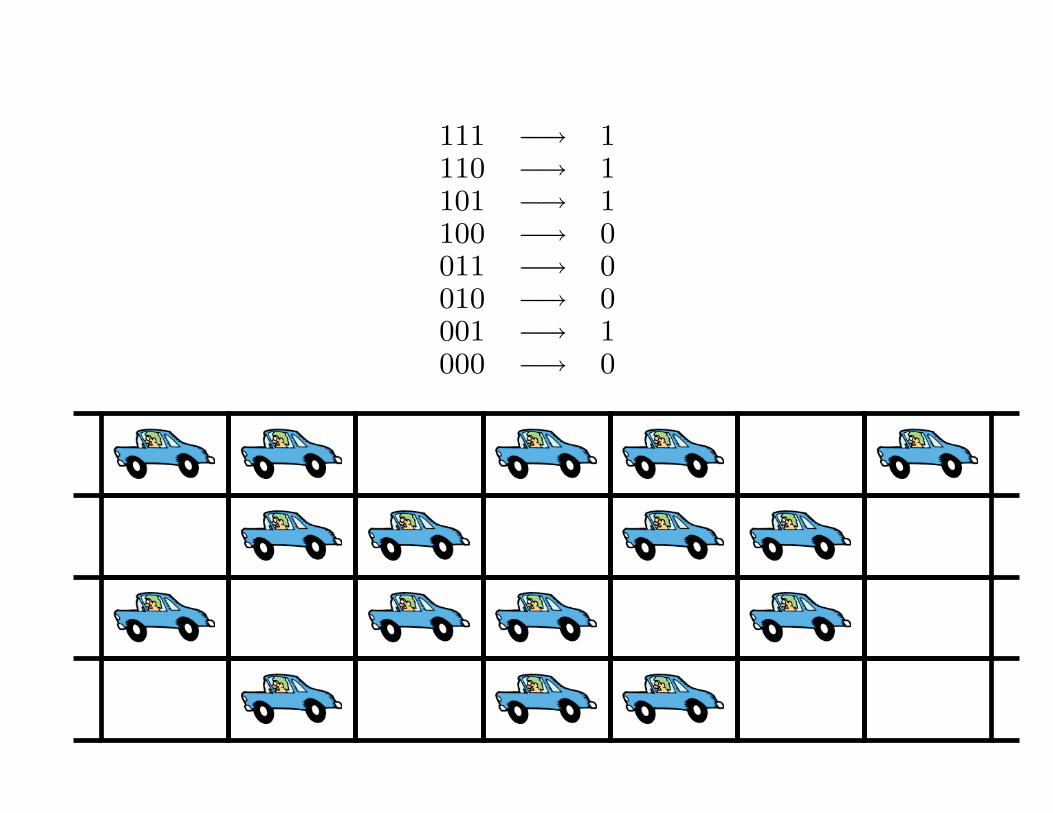
The Traffic CA is the elementary CA number 226.
111 −→ 1110 −→ 1101 −→ 1100 −→ 0011 −→ 0010 −→ 0001 −→ 1000 −→ 0
The local rule replaces pattern 01 by pattern 10.
111 −→ 1110 −→ 1101 −→ 1100 −→ 0011 −→ 0010 −→ 0001 −→ 1000 −→ 0
111 −→ 1110 −→ 1101 −→ 1100 −→ 0011 −→ 0010 −→ 0001 −→ 1000 −→ 0
111 −→ 1110 −→ 1101 −→ 1100 −→ 0011 −→ 0010 −→ 0001 −→ 1000 −→ 0
111 −→ 1110 −→ 1101 −→ 1100 −→ 0011 −→ 0010 −→ 0001 −→ 1000 −→ 0
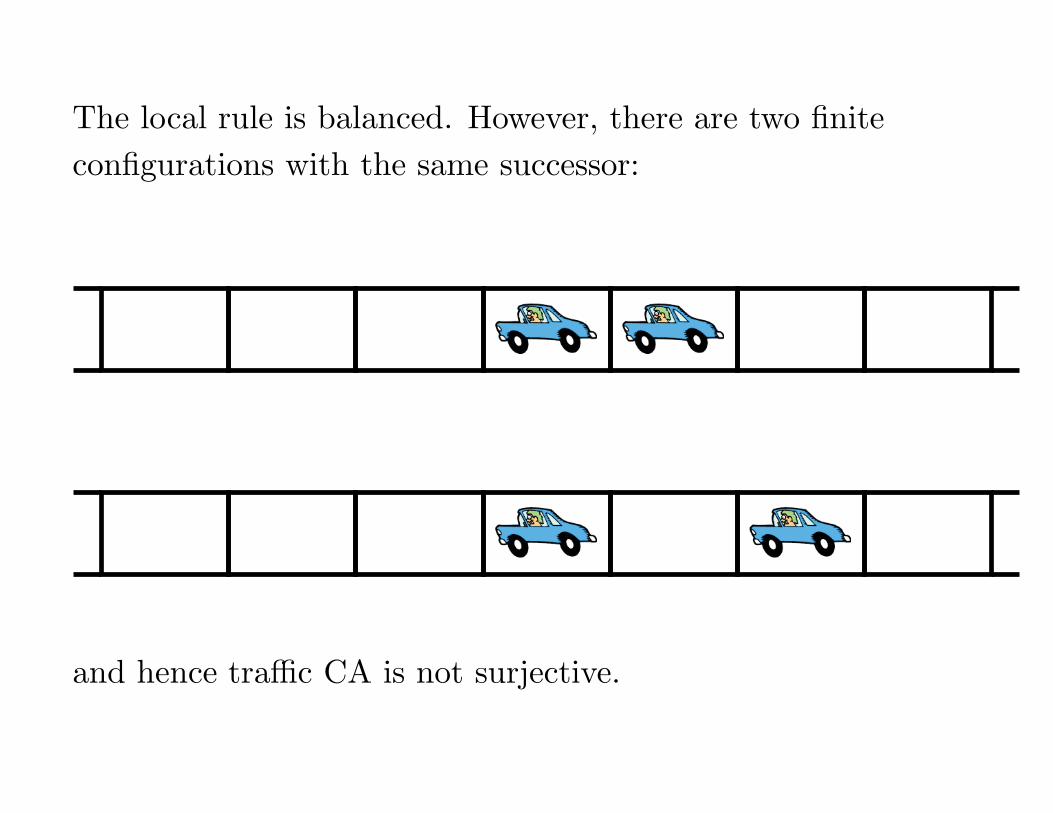
The local rule is balanced. However, there are two finite
configurations with the same successor:
and hence traffic CA is not surjective.
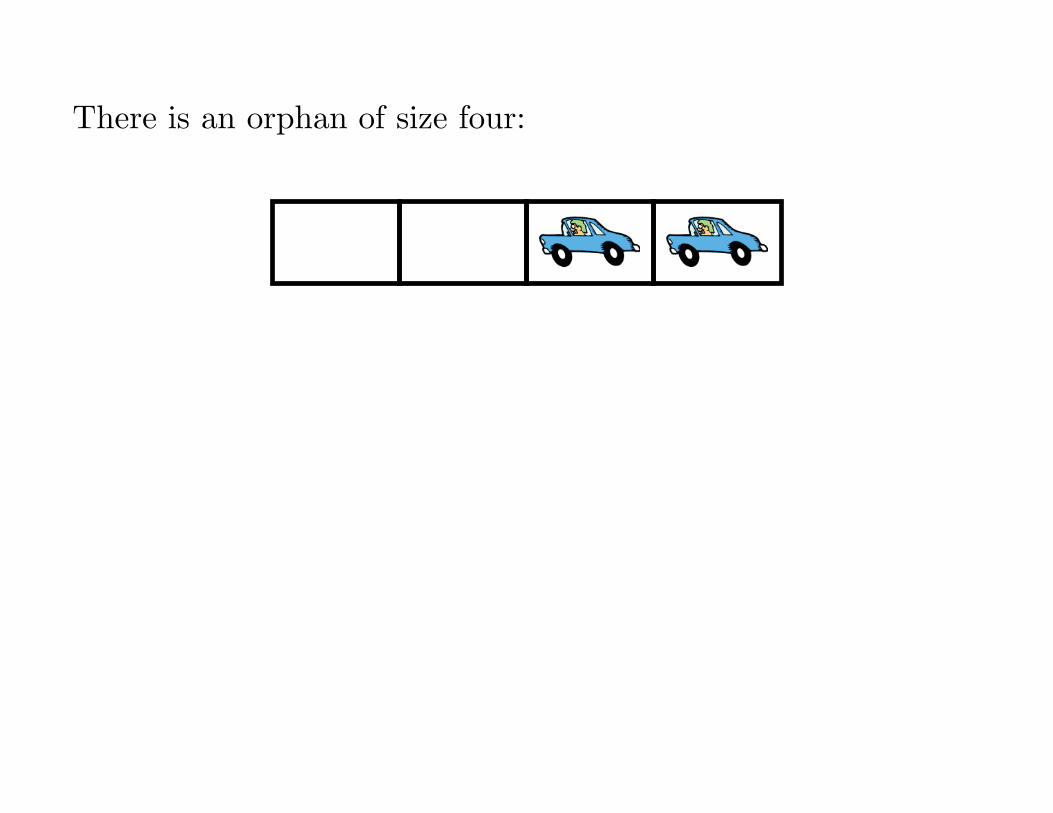
There is an orphan of size four:
Outline of the talk(s)
(1) Definitions (configurations, neighborhoods, cellular
automata, reversibility, injectivity, surjectivity)
(2) Classical results (Hedlund’s theorem, balance in
surjective CA, Garden-Of-Eden theorem)
(3) Reversible CA (universality, billiard ball CA)
(4) Decidability questions (Wang tiles, domino problem,
snake tiles, undecidability of nilpotency, reversibility,
surjectivity, periodicity)
(5) Dynamical systems aspects (equicontinuity
classification, limit sets)
Reversible cellular automata (RCA)
Reversibility is an important aspect of physics at the
microscopic scale, so it is natural that simulations are done
using reversible CA. Despite being a very restrictive condition,
reversibility does not prevent universal computation.
It is clear that any Turing machine can be simulated by a
one-dimensional CA. In 1977 T.Toffoli demonstrated how any
d-dimensional CA can be simulated by a d + 1-dimensional
RCA. Hence two-dimensional universal RCA exist.
In 1989 K.Morita and M.Harao showed how to simulate any
reversible Turing machine by a one-dimensional RCA. Since
reversible Turing machines can be computation universal
(Bennett 1973), the following result follows:
Theorem: One-dimensional reversible cellular automata exist
that are computationally universal.
In the following I give a simple construction of a
one-dimensional reversible CA that simulates in real time any
Turing machine, reversible or not.
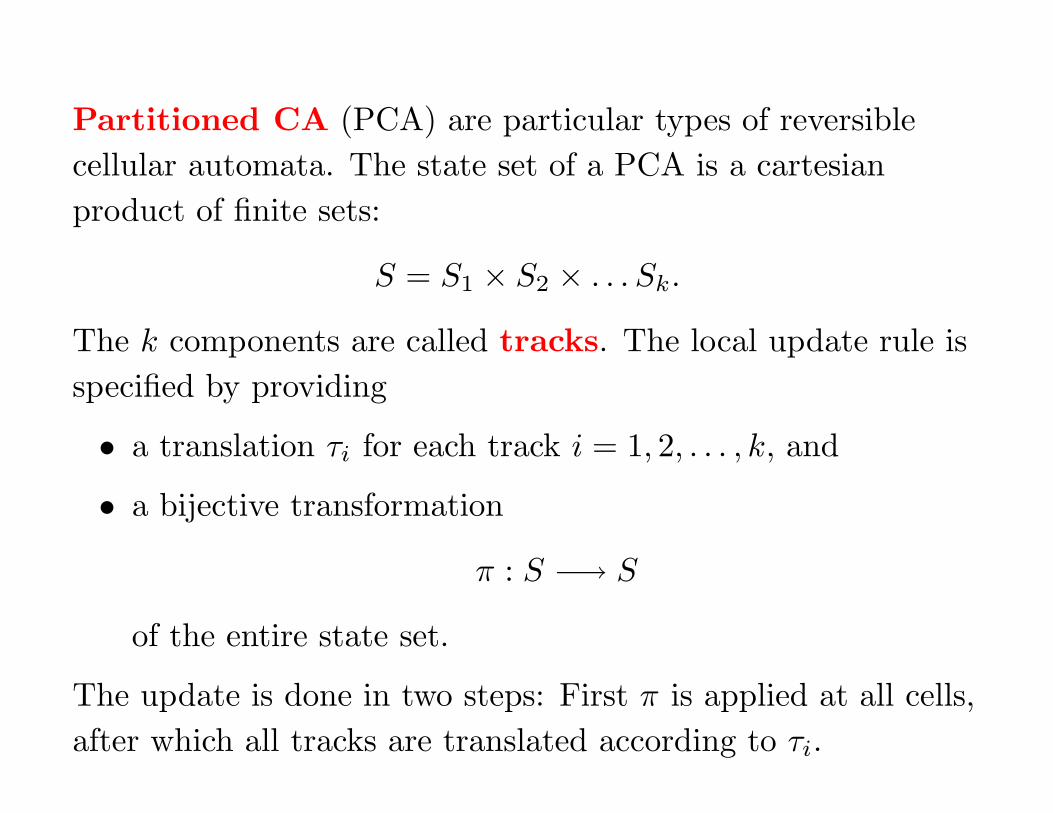
Partitioned CA (PCA) are particular types of reversible
cellular automata. The state set of a PCA is a cartesian
product of finite sets:
S = S1 × S2 × . . . Sk.
The k components are called tracks. The local update rule is
specified by providing
• a translation τi for each track i = 1, 2, . . . , k, and
• a bijective transformation
π : S −→ S
of the entire state set.
The update is done in two steps: First π is applied at all cells,
after which all tracks are translated according to τi.
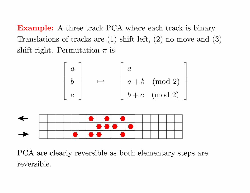
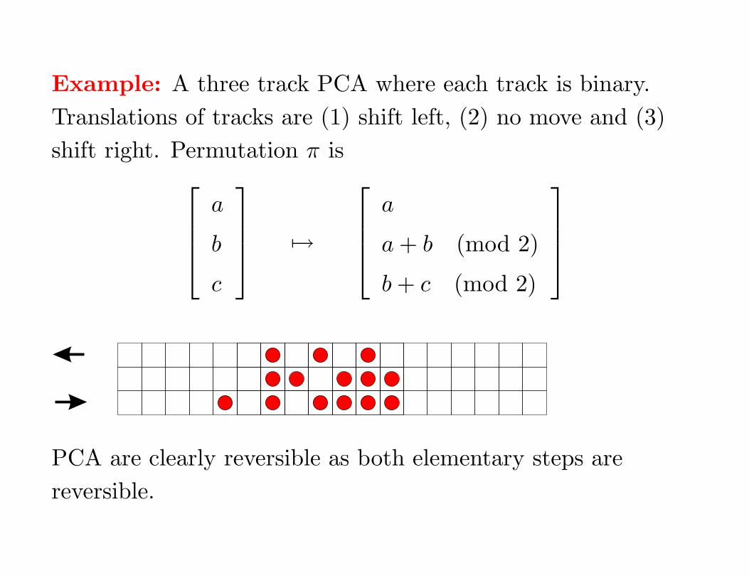
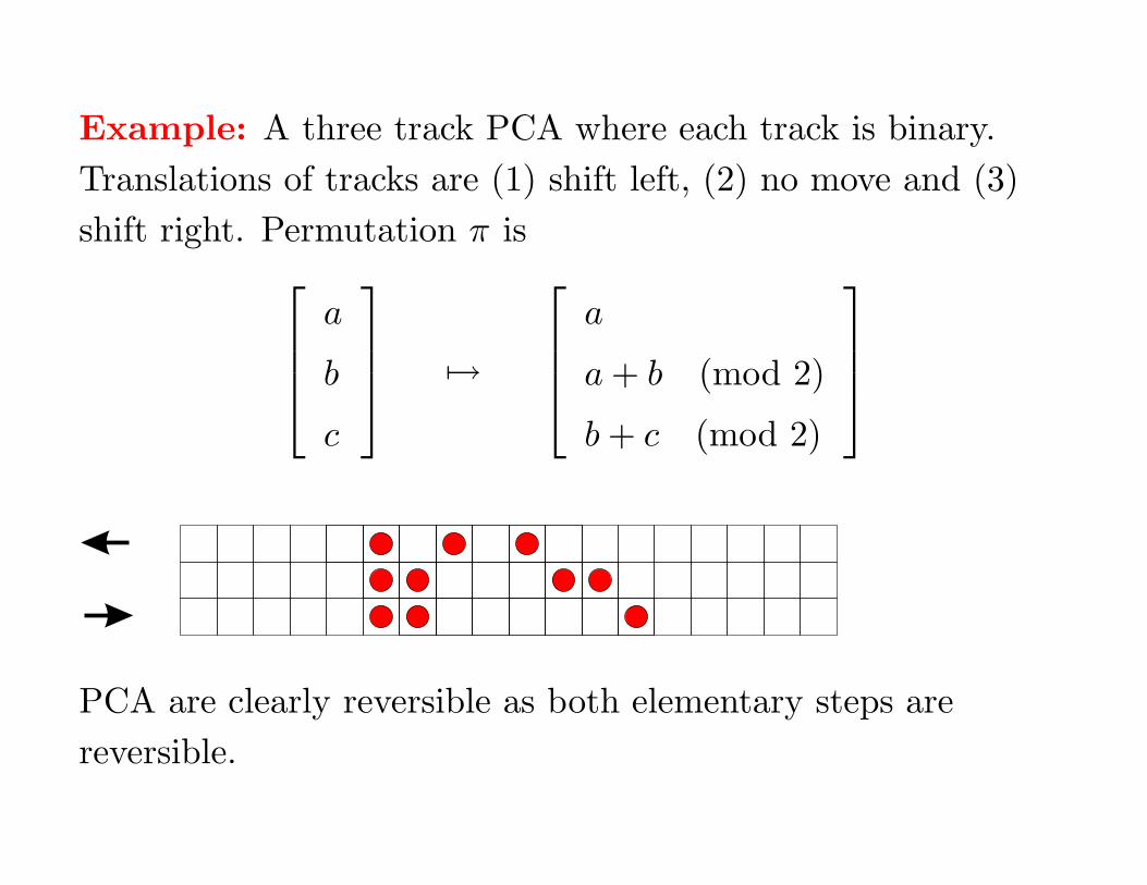
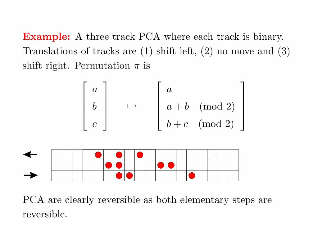
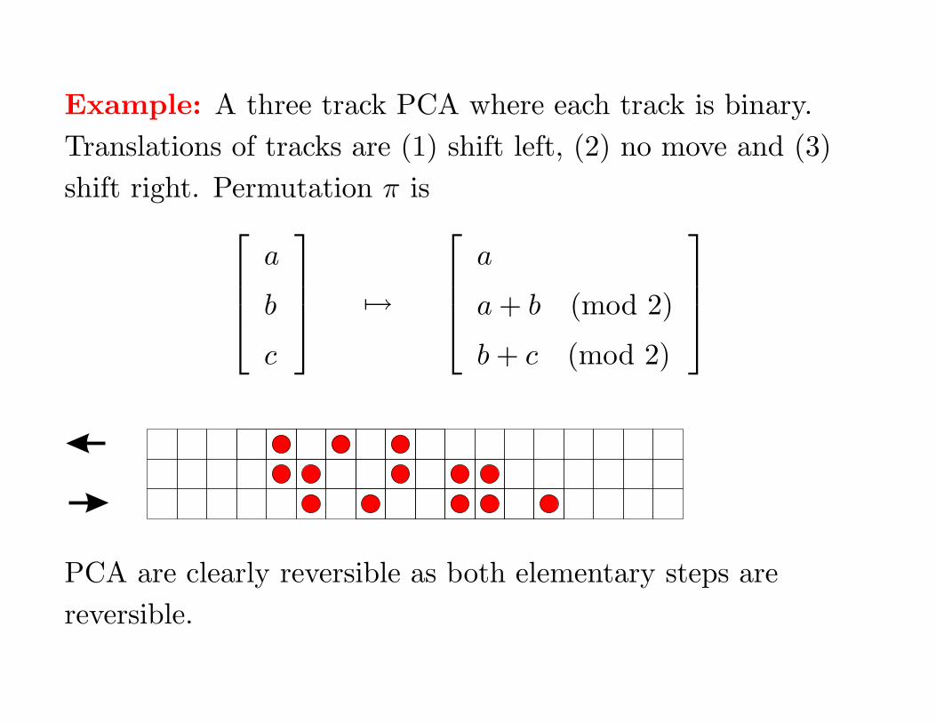
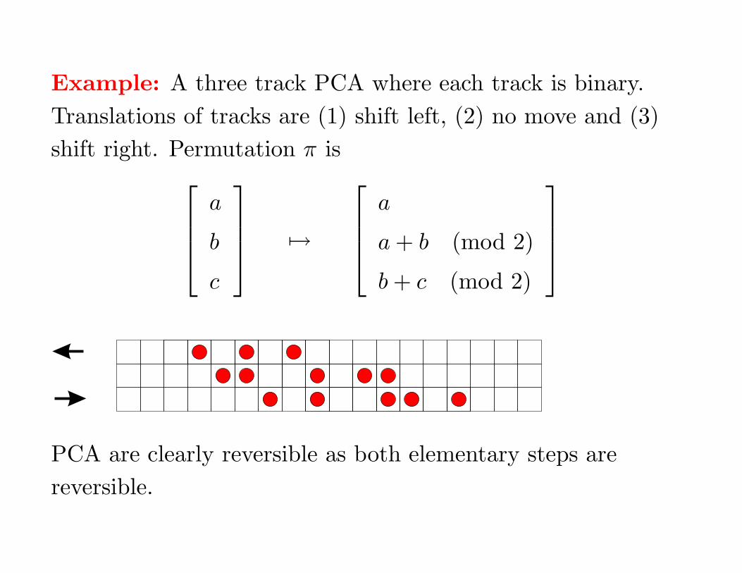
Example: A three track PCA where each track is binary.
Translations of tracks are (1) shift left, (2) no move and (3)
shift right. Permutation π is
a
b
c
7→
a
a + b (mod 2)
b + c (mod 2)
PCA are clearly reversible as both elementary steps are
reversible.
Example: A three track PCA where each track is binary.
Translations of tracks are (1) shift left, (2) no move and (3)
shift right. Permutation π is
a
b
c
7→
a
a + b (mod 2)
b + c (mod 2)
PCA are clearly reversible as both elementary steps are
reversible.

Example: A three track PCA where each track is binary.
Translations of tracks are (1) shift left, (2) no move and (3)
shift right. Permutation π is
a
b
c
7→
a
a + b (mod 2)
b + c (mod 2)
PCA are clearly reversible as both elementary steps are
reversible.
Example: A three track PCA where each track is binary.
Translations of tracks are (1) shift left, (2) no move and (3)
shift right. Permutation π is
a
b
c
7→
a
a + b (mod 2)
b + c (mod 2)
PCA are clearly reversible as both elementary steps are
reversible.
Example: A three track PCA where each track is binary.
Translations of tracks are (1) shift left, (2) no move and (3)
shift right. Permutation π is
a
b
c
7→
a
a + b (mod 2)
b + c (mod 2)
PCA are clearly reversible as both elementary steps are
reversible.
Example: A three track PCA where each track is binary.
Translations of tracks are (1) shift left, (2) no move and (3)
shift right. Permutation π is
a
b
c
7→
a
a + b (mod 2)
b + c (mod 2)
PCA are clearly reversible as both elementary steps are
reversible.
Example: A three track PCA where each track is binary.
Translations of tracks are (1) shift left, (2) no move and (3)
shift right. Permutation π is
a
b
c
7→
a
a + b (mod 2)
b + c (mod 2)
PCA are clearly reversible as both elementary steps are
reversible.
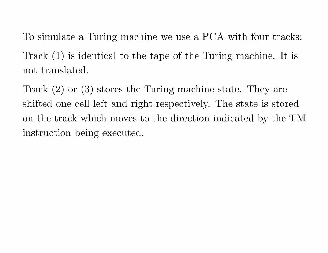
To simulate a Turing machine we use a PCA with four tracks:
Track (1) is identical to the tape of the Turing machine. It is
not translated.
To simulate a Turing machine we use a PCA with four tracks:
Track (1) is identical to the tape of the Turing machine. It is
not translated.
Track (2) or (3) stores the Turing machine state. They are
shifted one cell left and right respectively. The state is stored
on the track which moves to the direction indicated by the TM
instruction being executed.
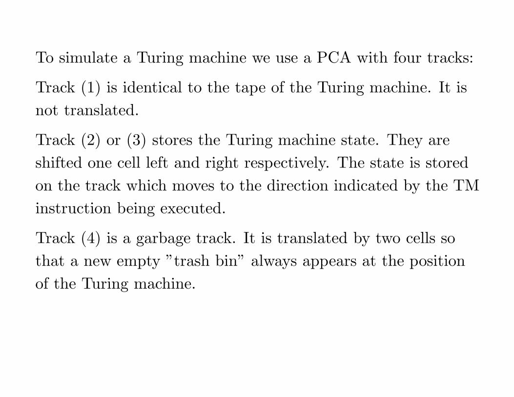
Track (4) is a garbage track. It is translated by two cells so
that a new empty ”trash bin” always appears at the position
of the Turing machine.
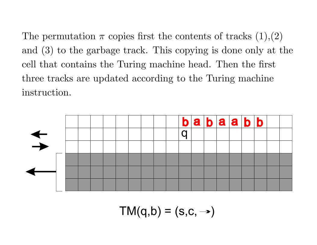
The permutation π copies first the contents of tracks (1),(2)
and (3) to the garbage track. This copying is done only at the
cell that contains the Turing machine head. Then the first
three tracks are updated according to the Turing machine
instruction.
a a ab b b bq
TM(q,b) = (s,c, )

The permutation π copies first the contents of tracks (1),(2)
and (3) to the garbage track. This copying is done only at the
cell that contains the Turing machine head. Then the first
three tracks are updated according to the Turing machine
instruction.
bq
a a ac b b b
s
TM(q,b) = (s,c, )

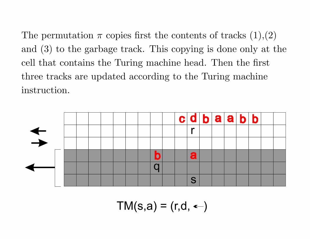
The permutation π copies first the contents of tracks (1),(2)
and (3) to the garbage track. This copying is done only at the
cell that contains the Turing machine head. Then the first
three tracks are updated according to the Turing machine
instruction.
a a ac b b b
s
TM(s,a) = (r,d, )
bq
The permutation π copies first the contents of tracks (1),(2)
and (3) to the garbage track. This copying is done only at the
cell that contains the Turing machine head. Then the first
three tracks are updated according to the Turing machine
instruction.
a
a ac b b b
s
TM(s,a) = (r,d, )
bq
dr
s
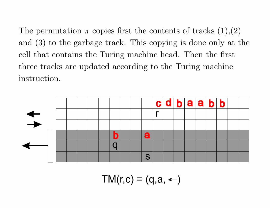
The permutation π copies first the contents of tracks (1),(2)
and (3) to the garbage track. This copying is done only at the
cell that contains the Turing machine head. Then the first
three tracks are updated according to the Turing machine
instruction.
a
a ac b b b
s
TM(r,c) = (q,a, )
bq
dr
s
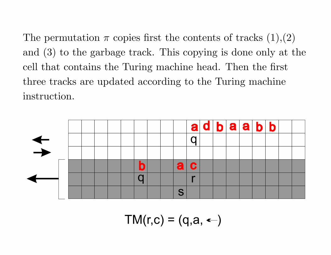
The permutation π copies first the contents of tracks (1),(2)
and (3) to the garbage track. This copying is done only at the
cell that contains the Turing machine head. Then the first
three tracks are updated according to the Turing machine
instruction.
a
a aa b b b
s
TM(r,c) = (q,a, )
bq
dq
s
cr

The permutation π copies first the contents of tracks (1),(2)
and (3) to the garbage track. This copying is done only at the
cell that contains the Turing machine head. Then the first
three tracks are updated according to the Turing machine
instruction.
a
a aa b b b
s
TM(q, ) = (r,a, )
bq
dq
s
cr

The permutation π copies first the contents of tracks (1),(2)
and (3) to the garbage track. This copying is done only at the
cell that contains the Turing machine head. Then the first
three tracks are updated according to the Turing machine
instruction.
a
a aa b b b
s
TM(q, ) = (r,a, )
bq
d
r
s
cr q
a

The permutation π copies first the contents of tracks (1),(2)
and (3) to the garbage track. This copying is done only at the
cell that contains the Turing machine head. Then the first
three tracks are updated according to the Turing machine
instruction.
a
a aa b b b
s
TM(r, a) = (s,d, )
bq
d
r
s
cr q
a
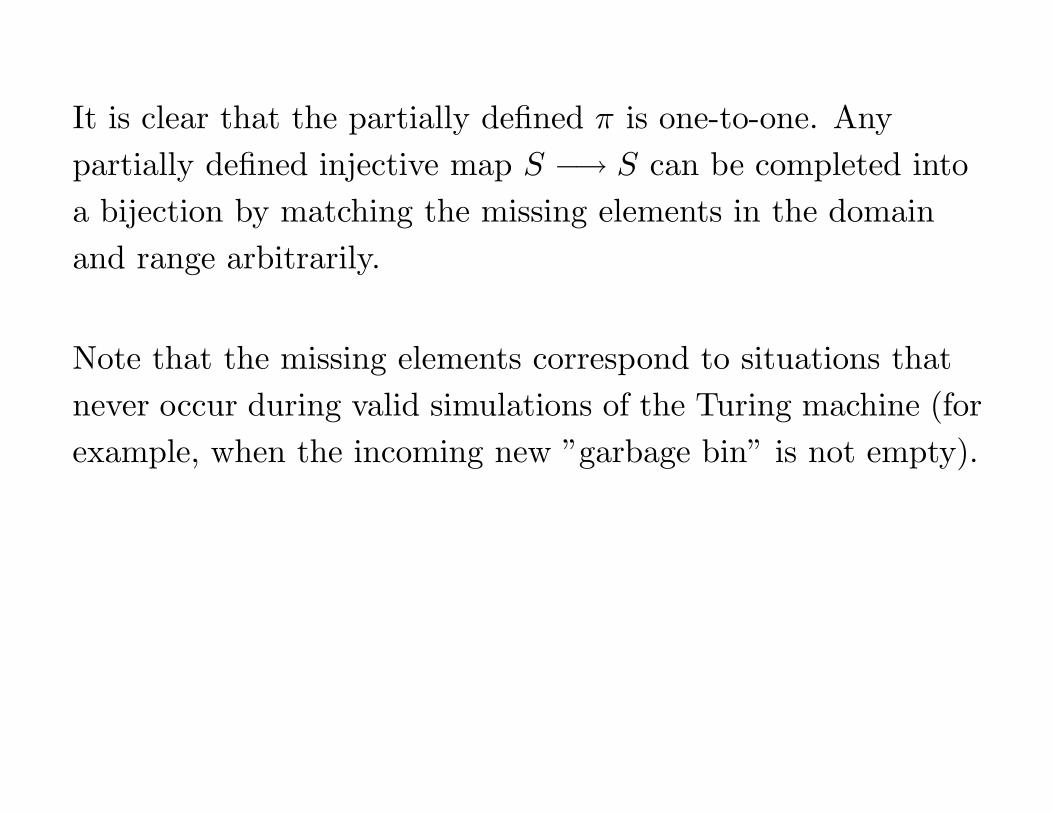
It is clear that the partially defined π is one-to-one. Any
partially defined injective map S −→ S can be completed into
a bijection by matching the missing elements in the domain
and range arbitrarily.
Note that the missing elements correspond to situations that
never occur during valid simulations of the Turing machine (for
example, when the incoming new ”garbage bin” is not empty).
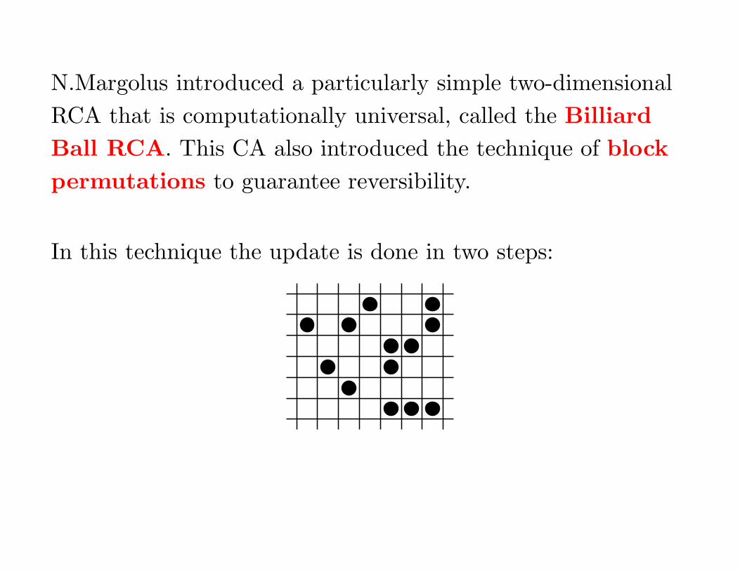
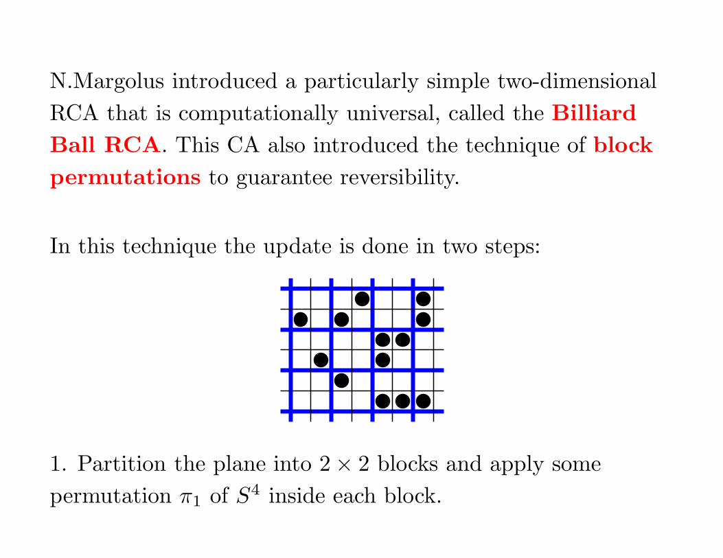
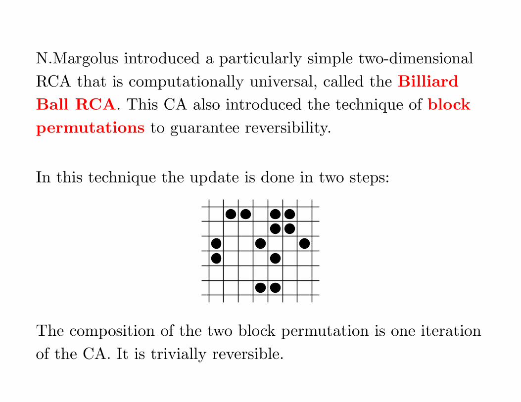
N.Margolus introduced a particularly simple two-dimensional
RCA that is computationally universal, called the Billiard
Ball RCA. This CA also introduced the technique of block
permutations to guarantee reversibility.
In this technique the update is done in two steps:
������������������������
����������������
��������
����������������
��������
��������
������������������������
1. Partition the plane into 2 × 2 blocks and apply some
permutation π1 of S4 inside each block.
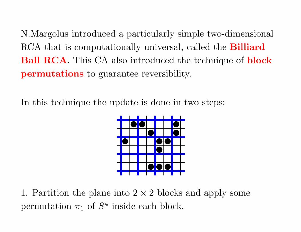
N.Margolus introduced a particularly simple two-dimensional
RCA that is computationally universal, called the Billiard
Ball RCA. This CA also introduced the technique of block
permutations to guarantee reversibility.
In this technique the update is done in two steps:
����������������
��������
����������������
����������������
����������������
��������
��������
��������
1. Partition the plane into 2 × 2 blocks and apply some
permutation π1 of S4 inside each block.
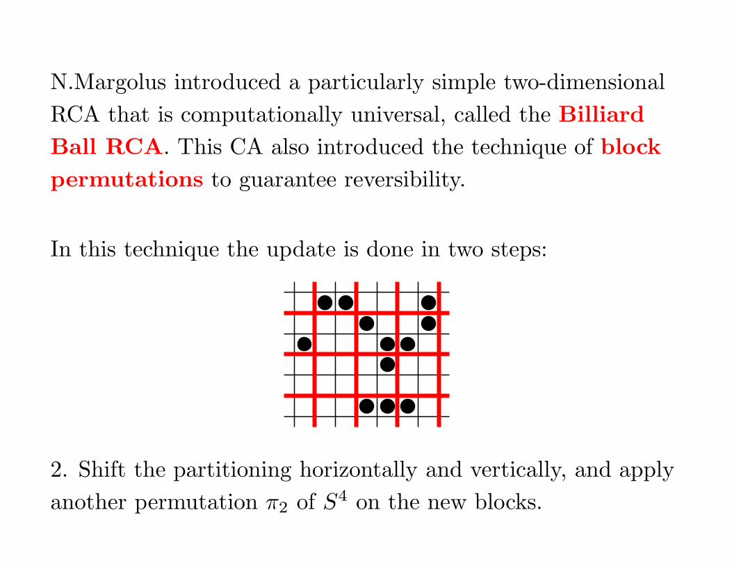
N.Margolus introduced a particularly simple two-dimensional
RCA that is computationally universal, called the Billiard
Ball RCA. This CA also introduced the technique of block
permutations to guarantee reversibility.
In this technique the update is done in two steps:
����������������
��������
����������������
����������������
����������������
��������
��������
��������
2. Shift the partitioning horizontally and vertically, and apply
another permutation π2 of S4 on the new blocks.
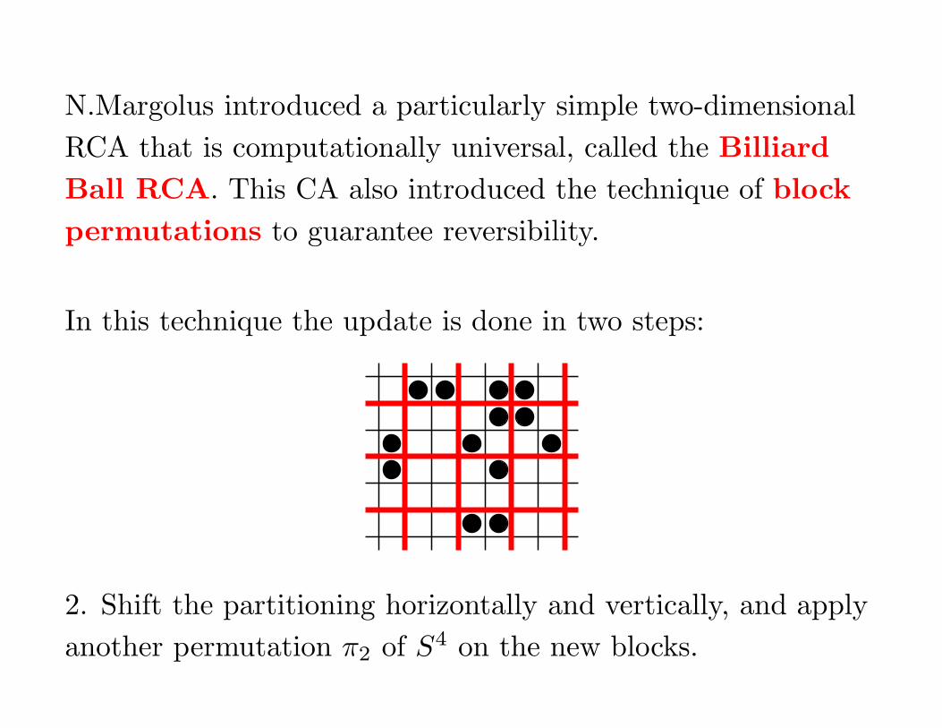
N.Margolus introduced a particularly simple two-dimensional
RCA that is computationally universal, called the Billiard
Ball RCA. This CA also introduced the technique of block
permutations to guarantee reversibility.
In this technique the update is done in two steps:
��������
��������
����������������
��������
��������
������������������������
��������
����������������
��������
2. Shift the partitioning horizontally and vertically, and apply
another permutation π2 of S4 on the new blocks.
N.Margolus introduced a particularly simple two-dimensional
RCA that is computationally universal, called the Billiard
Ball RCA. This CA also introduced the technique of block
permutations to guarantee reversibility.
In this technique the update is done in two steps:
��������
��������
����������������
��������������������������������
��������
����������������
��������
��������
The composition of the two block permutation is one iteration
of the CA. It is trivially reversible.
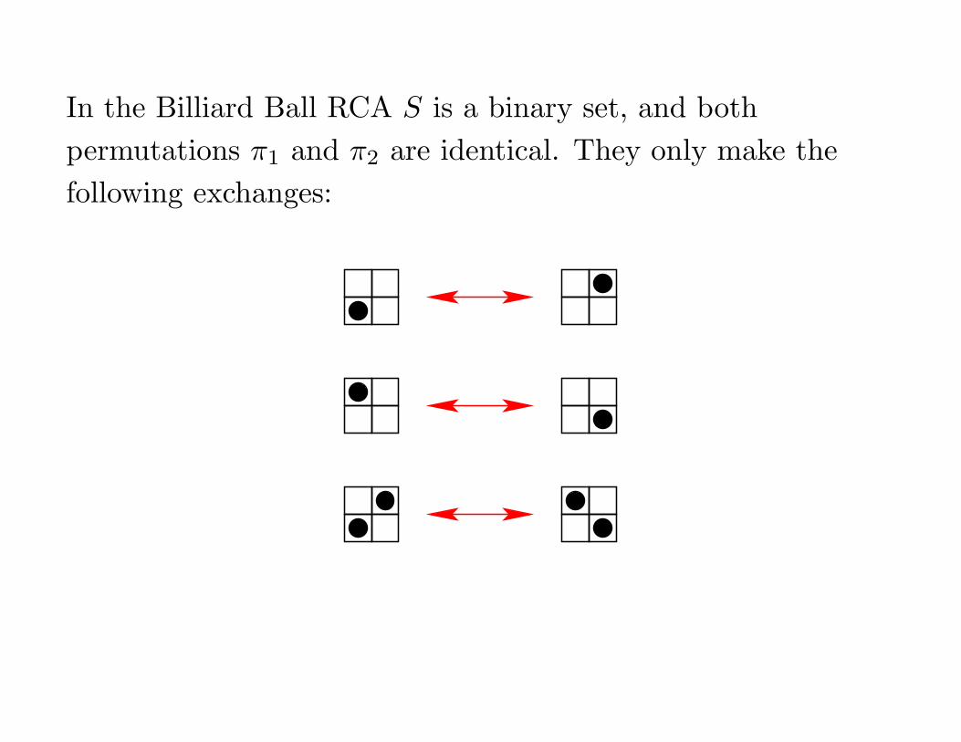
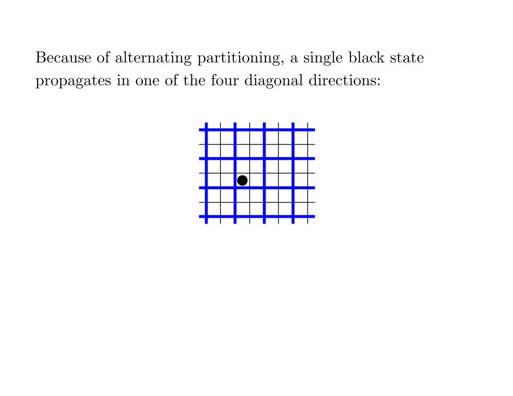
In the Billiard Ball RCA S is a binary set, and both
permutations π1 and π2 are identical. They only make the
following exchanges:
�������� ��
������
��������
��������
����������������
��������
��������
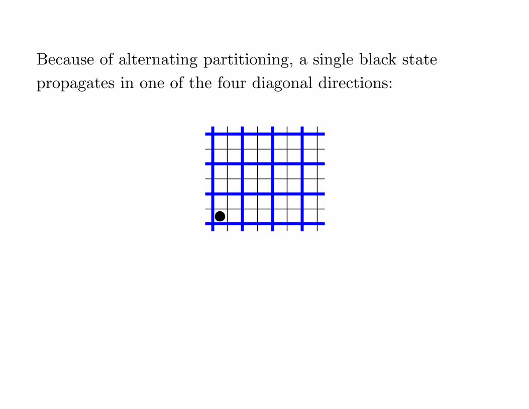
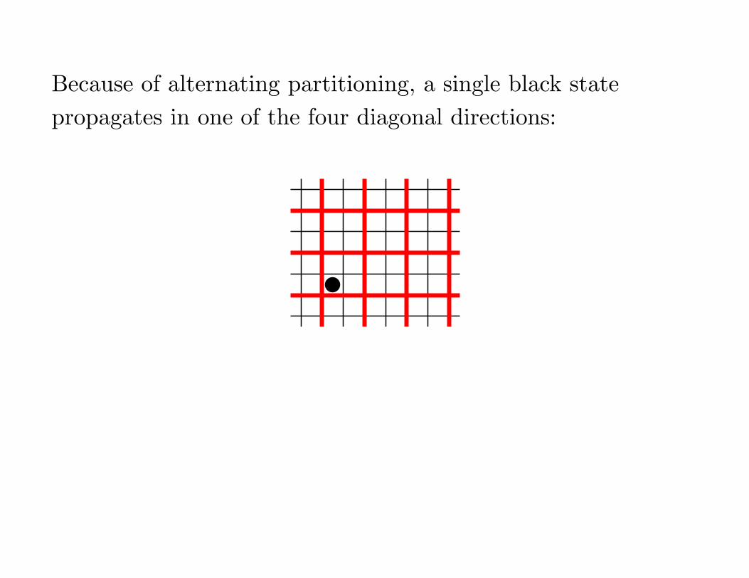
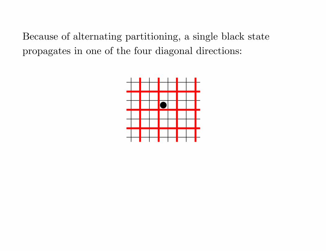
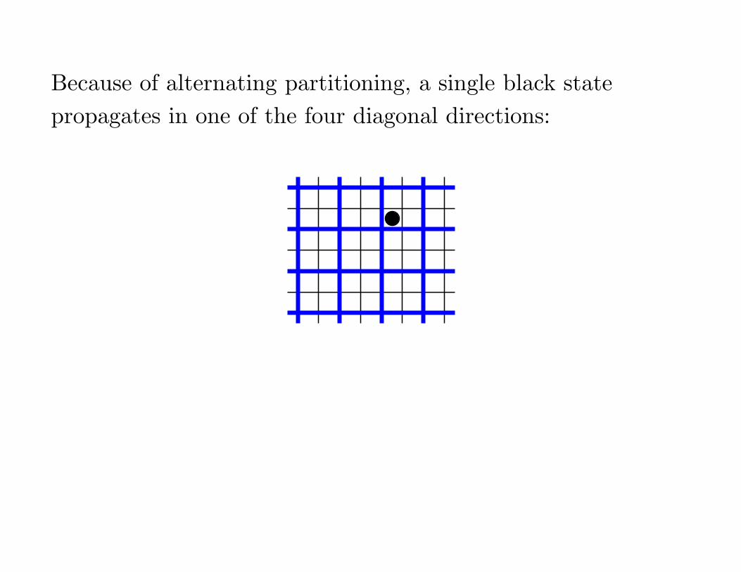
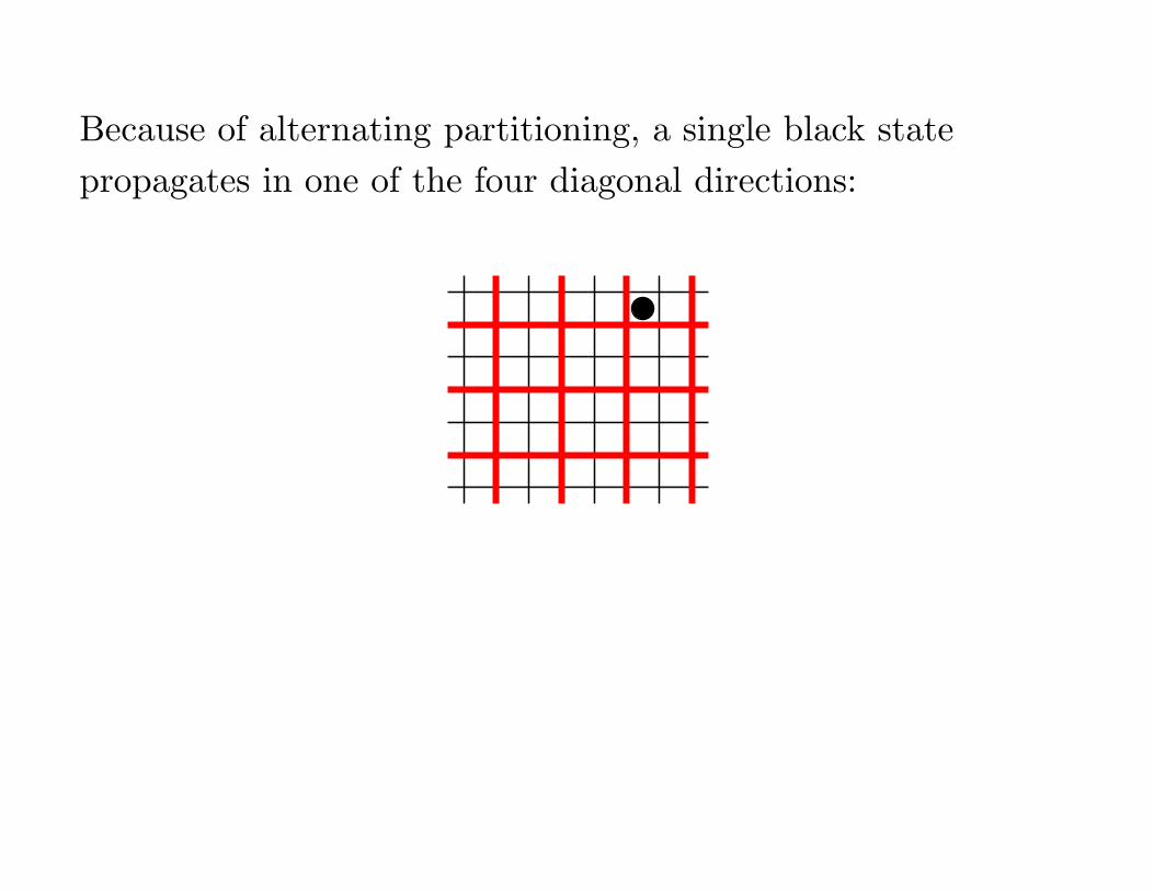
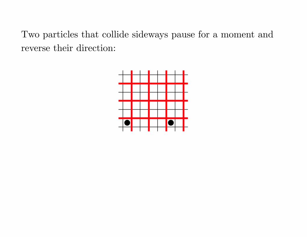
Because of alternating partitioning, a single black state
propagates in one of the four diagonal directions:
��������
Because of alternating partitioning, a single black state
propagates in one of the four diagonal directions:
��������
Because of alternating partitioning, a single black state
propagates in one of the four diagonal directions:
��������
Because of alternating partitioning, a single black state
propagates in one of the four diagonal directions:
��������
Because of alternating partitioning, a single black state
propagates in one of the four diagonal directions:
��������
Because of alternating partitioning, a single black state
propagates in one of the four diagonal directions:
��������
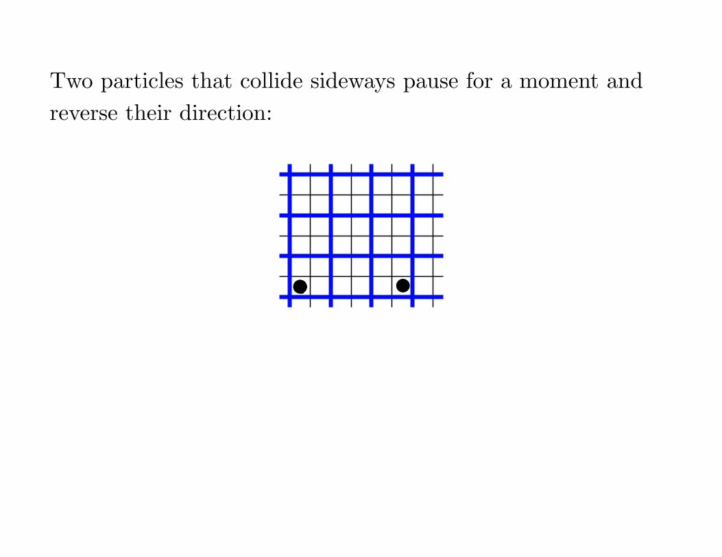
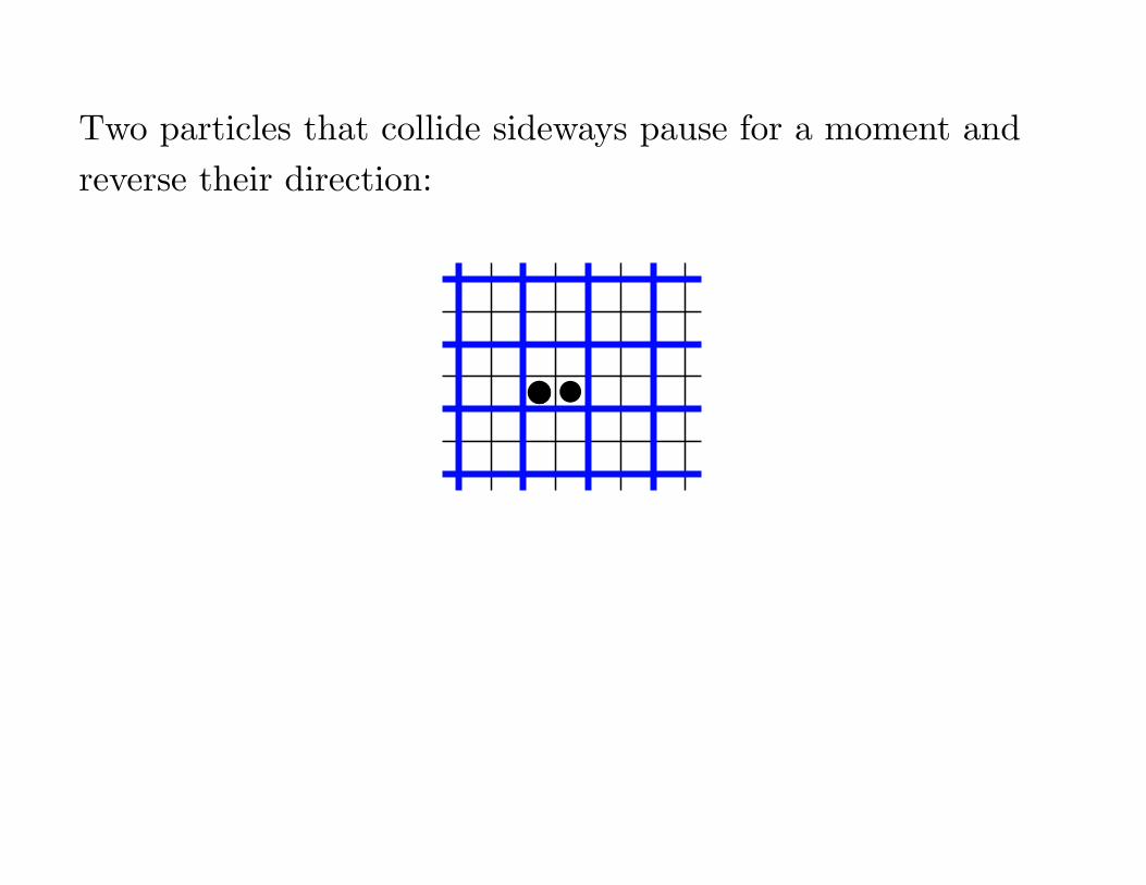
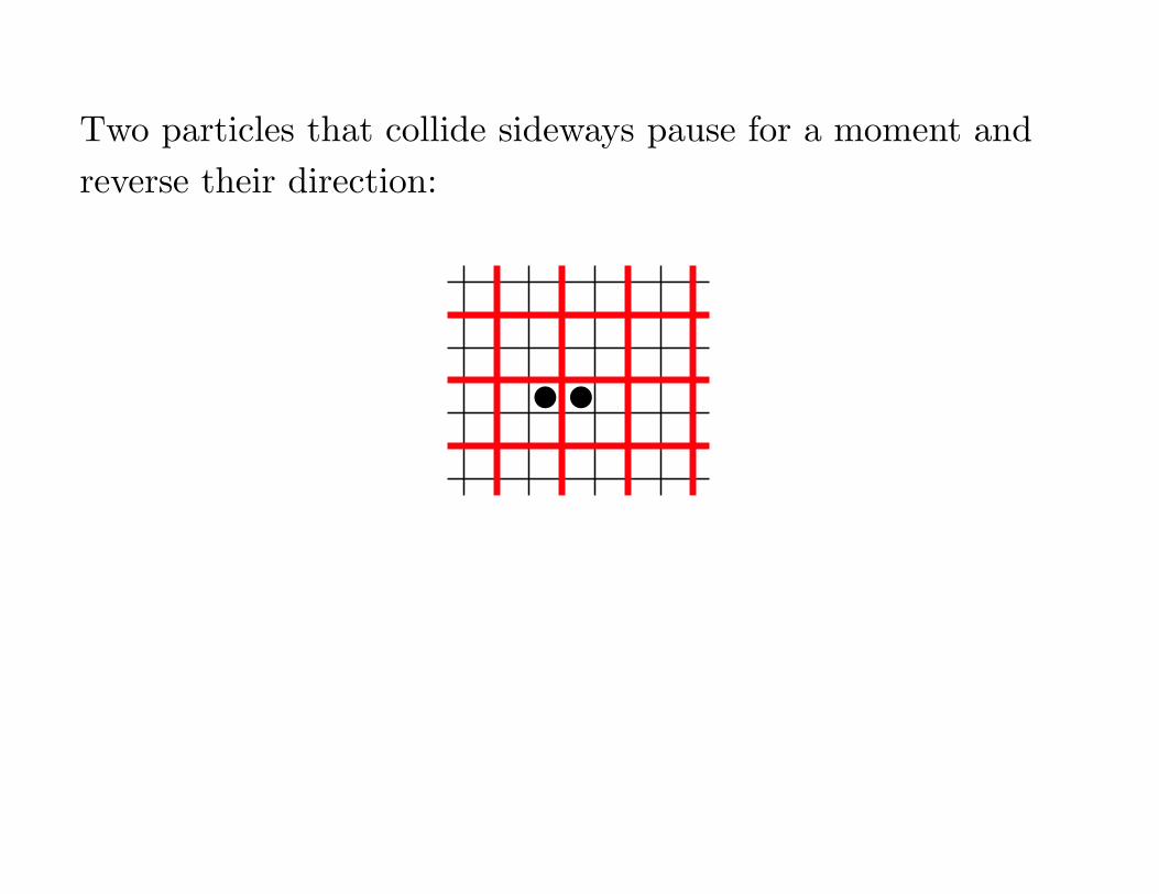
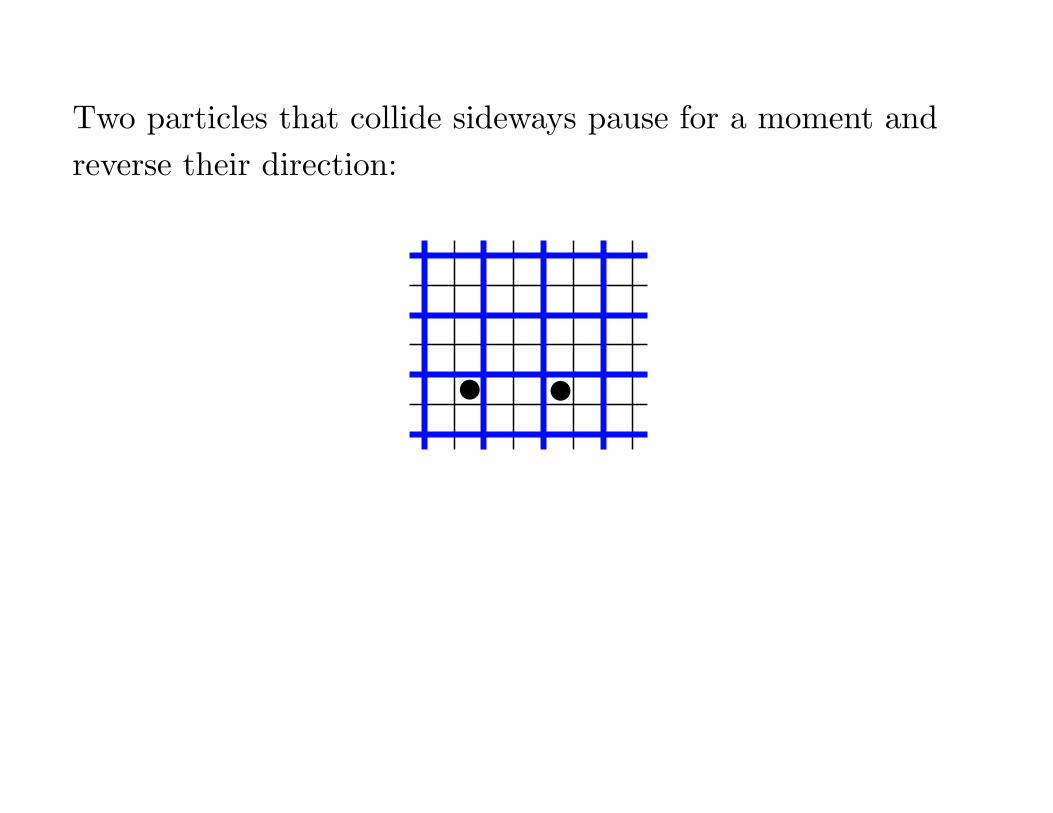
Two particles that collide sideways pause for a moment and
reverse their direction:

Two particles that collide sideways pause for a moment and
reverse their direction:
Two particles that collide sideways pause for a moment and
reverse their direction:
Two particles that collide sideways pause for a moment and
reverse their direction:
Two particles that collide sideways pause for a moment and
reverse their direction:
Two particles that collide sideways pause for a moment and
reverse their direction:
In the Billiard Ball RCA one can simulate the motion and
collisions of balls of positive diameter. Walls from which the
balls bounce can also be created. Amazingly, these constructs
are sufficient to perform arbitrary computation, proving the
computational universality of the Billiard Ball RCA.
In the Billiard Ball RCA one can simulate the motion and
collisions of balls of positive diameter. Walls from which the
balls bounce can also be created. Amazingly, these constructs
are sufficient to perform arbitrary computation, proving the
computational universality of the Billiard Ball RCA.
Reversibility is trivially obtained using the block permutation
technique. Also conservation laws are easy to enforce. For
example, if the permutations π1 and π2 are such that they
preserve the numbers of black states (e.g. as in the Billiard
Ball RCA) then the whole CA conserves the number of black
states.
Reversible CA come up naturally when simulating reversible
physical systems.
Reversible CA come up naturally when simulating reversible
physical systems.
Conversely, physically building a cellular automata device in
the reversible physical universe is most energy efficient if the
CA is reversible. In fact, whenever a physical device erases
information (by performing, say, a logical AND operation) it
must dissipate energy from the system, usually in the form of
heat.
It is more energy efficient to use only reversible logical
operations during computation.
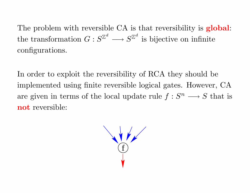
The problem with reversible CA is that reversibility is global:
the transformation G : SZd
−→ SZd
is bijective on infinite
configurations.
In order to exploit the reversibility of RCA they should be
implemented using finite reversible logical gates. However, CA
are given in terms of the local update rule f : Sn −→ S that is
not reversible:
f
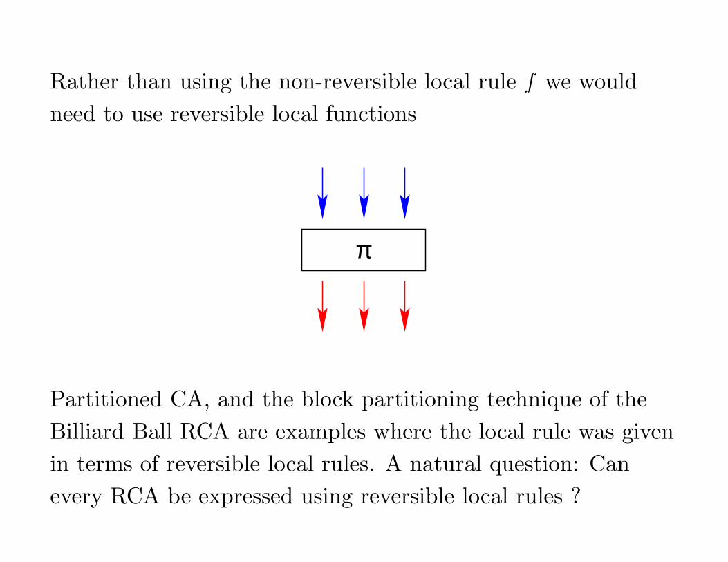
Rather than using the non-reversible local rule f we would
need to use reversible local functions
π
Partitioned CA, and the block partitioning technique of the
Billiard Ball RCA are examples where the local rule was given
in terms of reversible local rules. A natural question: Can
every RCA be expressed using reversible local rules ?
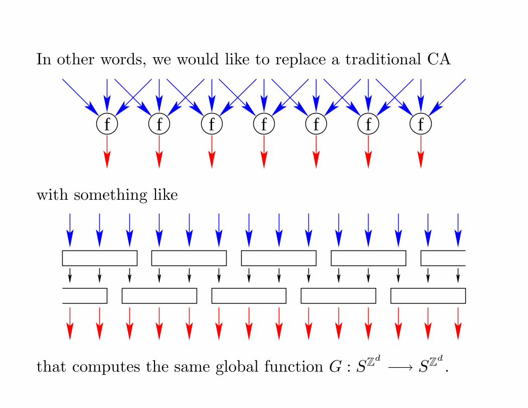
In other words, we would like to replace a traditional CA
f f f f fff
with something like
that computes the same global function G : SZd
−→ SZd
.
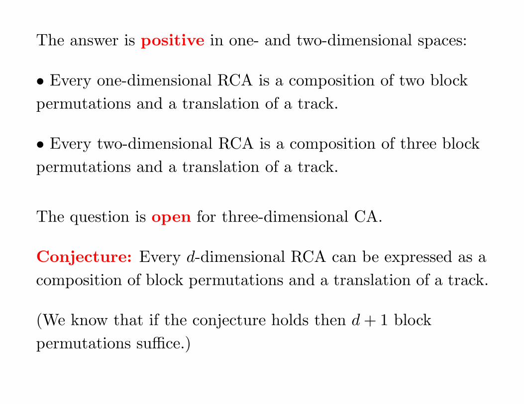
The answer is positive in one- and two-dimensional spaces:
• Every one-dimensional RCA is a composition of two block
permutations and a translation of a track.
The answer is positive in one- and two-dimensional spaces:
• Every one-dimensional RCA is a composition of two block
permutations and a translation of a track.
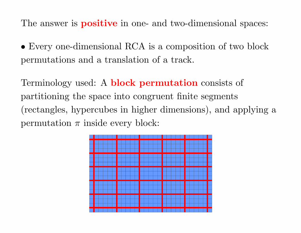
Terminology used: A block permutation consists of
partitioning the space into congruent finite segments
(rectangles, hypercubes in higher dimensions), and applying a
permutation π inside every block:
The answer is positive in one- and two-dimensional spaces:
• Every one-dimensional RCA is a composition of two block
permutations and a translation of a track.
Translating a track means expressing the state set as a
cartesian product
S = S1 × S2
and translating the S1-components.
The answer is positive in one- and two-dimensional spaces:
• Every one-dimensional RCA is a composition of two block
permutations and a translation of a track.
• Every two-dimensional RCA is a composition of three block
permutations and a translation of a track.
The answer is positive in one- and two-dimensional spaces:
• Every one-dimensional RCA is a composition of two block
permutations and a translation of a track.
• Every two-dimensional RCA is a composition of three block
permutations and a translation of a track.
The question is open for three-dimensional CA.
Conjecture: Every d-dimensional RCA can be expressed as a
composition of block permutations and a translation of a track.
(We know that if the conjecture holds then d + 1 block
permutations suffice.)
Outline of the talk(s)
(1) Definitions (configurations, neighborhoods, cellular
automata, reversibility, injectivity, surjectivity)
(2) Classical results (Hedlund’s theorem, balance in
surjective CA, Garden-Of-Eden theorem)
(3) Reversible CA (universality, billiard ball CA)
(4) Decidability questions (Wang tiles, domino problem,
snake tiles, undecidability of nilpotency, reversibility,
surjectivity, periodicity)
(5) Dynamical systems aspects (equicontinuity
classification, limit sets)
Decidability questions
Suppose we are given a CA (in terms of its local update rule)
and want to know if it is reversible or surjective ? Is there an
algorithm to decide this ? Or is there an algorithm to
determine if the dynamics of a given CA is trivial in the sense
that after a while all activity has died ?
It turns out that many such algorithmic problems are
undecidable. In some cases there is an algorithm for
one-dimensional CA while the two-dimensional case is
undecidable.
A useful tool to obtain undecidability results is the concept of
Wang tiles and the undecidable tiling problem.
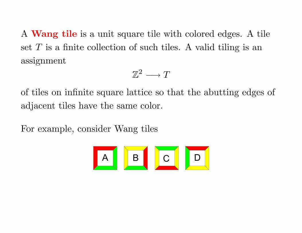
A Wang tile is a unit square tile with colored edges. A tile
set T is a finite collection of such tiles. A valid tiling is an
assignment
Z2 −→ T
of tiles on infinite square lattice so that the abutting edges of
adjacent tiles have the same color.
A B C D
A Wang tile is a unit square tile with colored edges. A tile
set T is a finite collection of such tiles. A valid tiling is an
assignment
Z2 −→ T
of tiles on infinite square lattice so that the abutting edges of
adjacent tiles have the same color.
For example, consider Wang tiles
A B C D
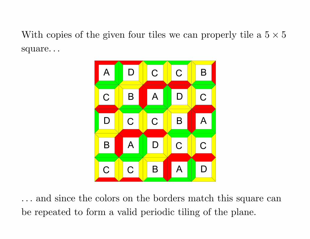
With copies of the given four tiles we can properly tile a 5 × 5
square. . .
A
B
C
D
C
A
C
B
D
C
B
D
A
C
C
B
D
C
A
C
B
A
C
D
C
. . . and since the colors on the borders match this square can
be repeated to form a valid periodic tiling of the plane.
The set of valid tilings using elements of T is a translation
invariant, compact subset of the configuration space T Z2
.
It is a two-dimensional counter-part of a subshift of finite
type used in symbolic dynamics, as it can be defined via a
finite collection of patterns that are not allowed in any valid
tiling.
We also use the following terminology: Configuration c ∈ T Z2
is valid inside M ⊆ Z2 if the colors match between any two
neighboring cells, both of which are inside region M .
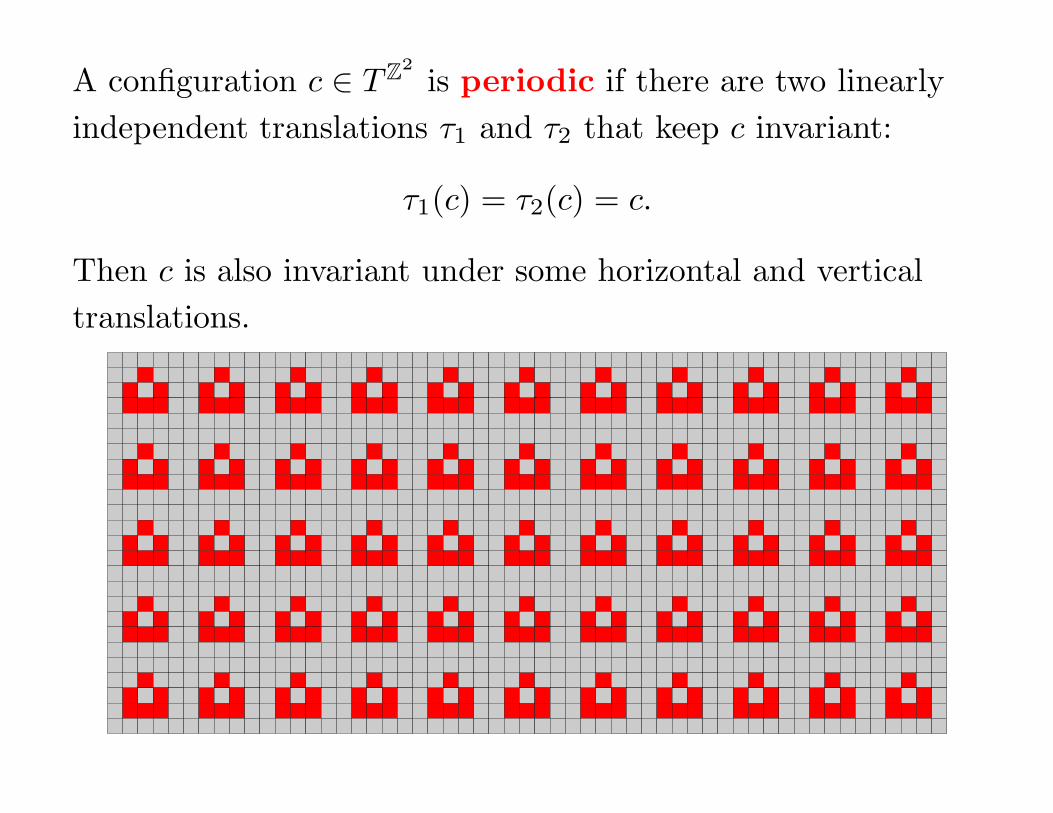
A configuration c ∈ T Z2
is periodic if there are two linearly
independent translations τ1 and τ2 that keep c invariant:
τ1(c) = τ2(c) = c.
Then c is also invariant under some horizontal and vertical
translations.
More generally, a d-dimensional configuration c ∈ SZd
is
periodic if it is invariant under d linearly independent
translations.
For d = 1 this is just the usual periodicity of infinite words.
The tiling problem of Wang tiles is the decision problem to
determine if a given finite set of Wang tiles admits a valid
tiling of the plane.
Theorem (R.Berger 1966): The tiling problem of Wang
tiles is undecidable.
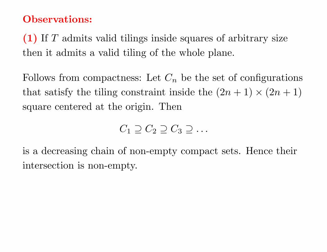
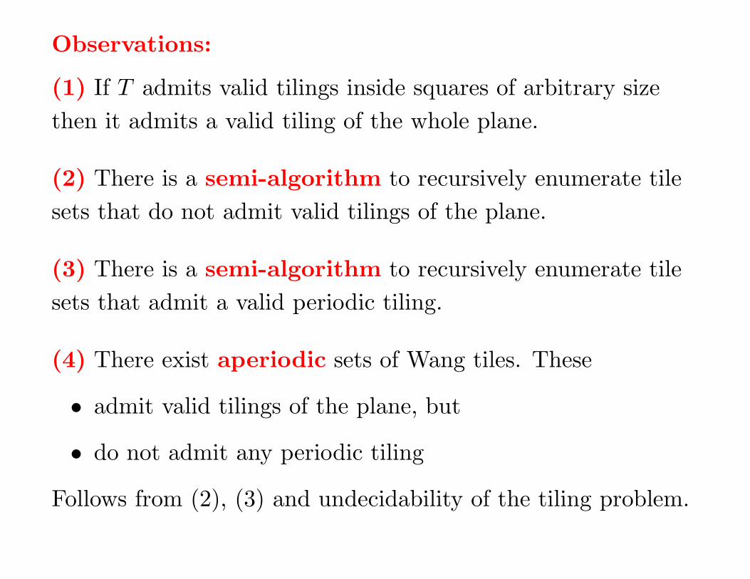
Observations:
(1) If T admits valid tilings inside squares of arbitrary size
then it admits a valid tiling of the whole plane.
Observations:
(1) If T admits valid tilings inside squares of arbitrary size
then it admits a valid tiling of the whole plane.
Follows from compactness: Let Cn be the set of configurations
that satisfy the tiling constraint inside the (2n + 1) × (2n + 1)
square centered at the origin. Then
C1 ⊇ C2 ⊇ C3 ⊇ . . .
is a decreasing chain of non-empty compact sets. Hence their
intersection is non-empty.
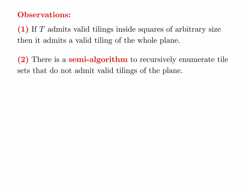
Observations:
(1) If T admits valid tilings inside squares of arbitrary size
then it admits a valid tiling of the whole plane.
(2) There is a semi-algorithm to recursively enumerate tile
sets that do not admit valid tilings of the plane.

Observations:
(1) If T admits valid tilings inside squares of arbitrary size
then it admits a valid tiling of the whole plane.
(2) There is a semi-algorithm to recursively enumerate tile
sets that do not admit valid tilings of the plane.
Follows from (1): Just try tiling larger and larger squares until
(if ever) a square is found that can not be tiled.
Observations:
(1) If T admits valid tilings inside squares of arbitrary size
then it admits a valid tiling of the whole plane.
(2) There is a semi-algorithm to recursively enumerate tile
sets that do not admit valid tilings of the plane.
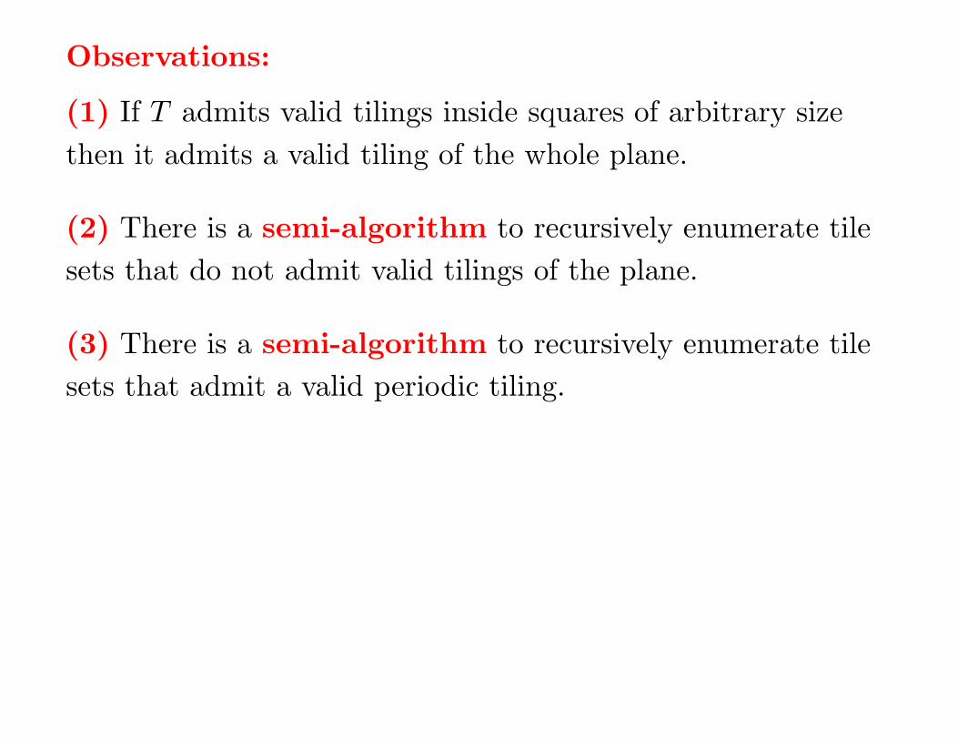
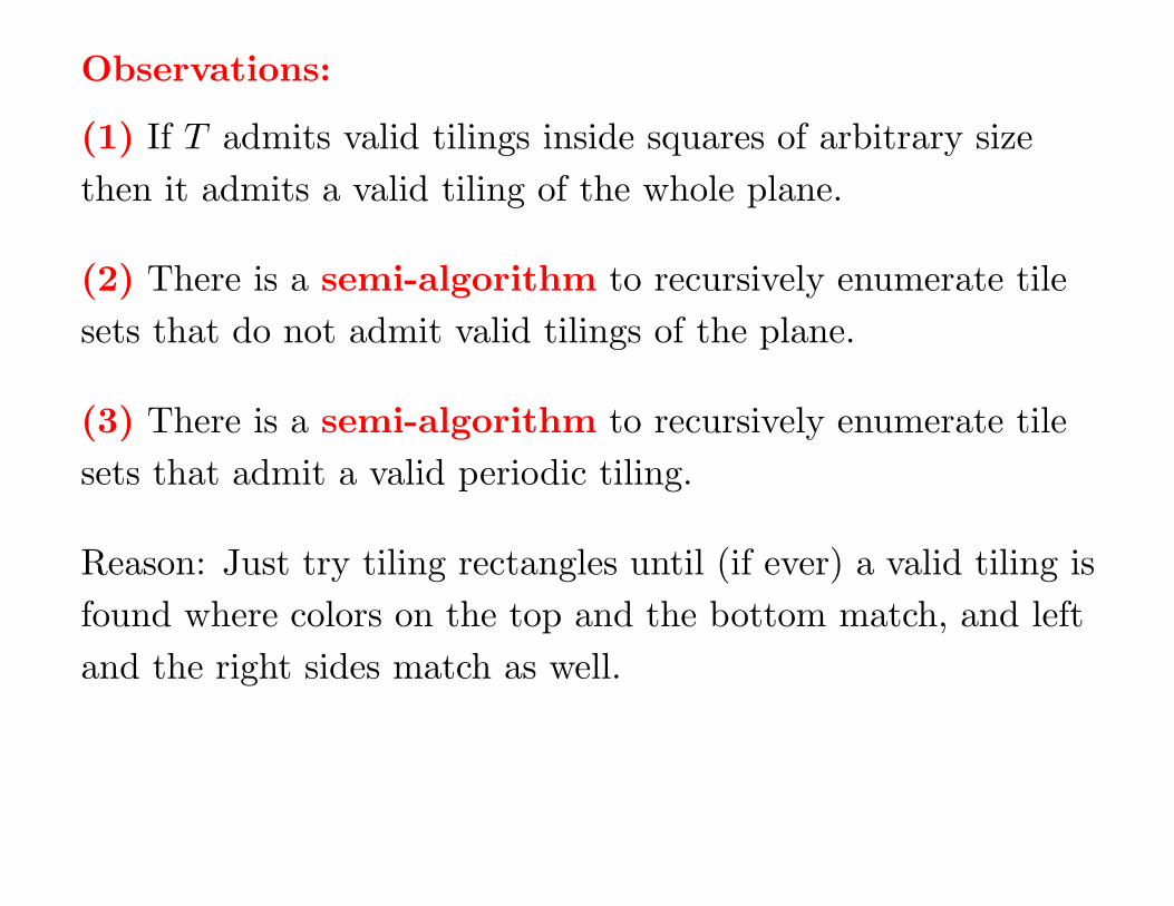
(3) There is a semi-algorithm to recursively enumerate tile
sets that admit a valid periodic tiling.
Observations:
(1) If T admits valid tilings inside squares of arbitrary size
then it admits a valid tiling of the whole plane.
(2) There is a semi-algorithm to recursively enumerate tile
sets that do not admit valid tilings of the plane.
(3) There is a semi-algorithm to recursively enumerate tile
sets that admit a valid periodic tiling.
Reason: Just try tiling rectangles until (if ever) a valid tiling is
found where colors on the top and the bottom match, and left
and the right sides match as well.

Observations:
(1) If T admits valid tilings inside squares of arbitrary size
then it admits a valid tiling of the whole plane.
(2) There is a semi-algorithm to recursively enumerate tile
sets that do not admit valid tilings of the plane.
(3) There is a semi-algorithm to recursively enumerate tile
sets that admit a valid periodic tiling.
(4) There exist aperiodic sets of Wang tiles. These
• admit valid tilings of the plane, but
• do not admit any periodic tiling
Follows from (2), (3) and undecidability of the tiling problem.
The tiling problem can be reduced to various decision
problems concerning (two-dimensional) cellular automata, so
that the undecidability of these problems then follows from
Berger’s result.
This is not so surprising since Wang tilings are ”static”
versions of ”dynamic” cellular automata.
Example: Let us prove that it is undecidable whether a given
two-dimensional CA G has any fixed point configurations, that
is, configurations c such that G(c) = c.
Proof: Reduction from the tiling problem. For any given
Wang tile set T (with at least two tiles) we effectively
construct a two-dimensional CA with state set T , the von
Neumann -neighborhood and a local update rule that keeps a
tile unchanged if and only if its colors match with the
neighboring tiles.
Trivially, G(c) = c if and only if c is a valid tiling.
Note: For one-dimensional CA it is decidable whether fixed
points exist. Fixed points form a subshift of finite type that
can be effectively constructed.
More interesting reduction: A CA is called nilpotent if all
configurations eventually evolve into the quiescent
configuration.
Observation: In a nilpotent CA all configurations must
become quiescent within a bounded time, that is, there is
number n such that Gn(c) is quiescent, for all c ∈ SZd
.
More interesting reduction: A CA is called nilpotent if all
configurations eventually evolve into the quiescent
configuration.
Observation: In a nilpotent CA all configurations must
become quiescent within a bounded time, that is, there is
number n such that Gn(c) is quiescent, for all c ∈ SZd
.
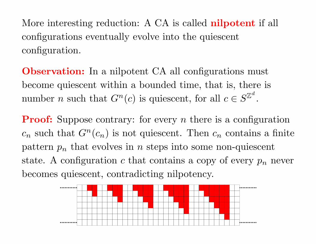
Proof: Suppose contrary: for every n there is a configuration
cn such that Gn(cn) is not quiescent. Then cn contains a finite
pattern pn that evolves in n steps into some non-quiescent
state. A configuration c that contains a copy of every pn never
becomes quiescent, contradicting nilpotency.
Theorem (Culik, Pachl, Yu, 1989): It is undecidable
whether a given two-dimensional CA is nilpotent.
Theorem (Culik, Pachl, Yu, 1989): It is undecidable
whether a given two-dimensional CA is nilpotent.
Proof: For any given set T of Wang tiles the goal is to
construct a two-dimensional CA that is nilpotent if and only if
T does not admit a tiling.
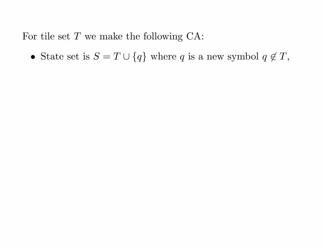
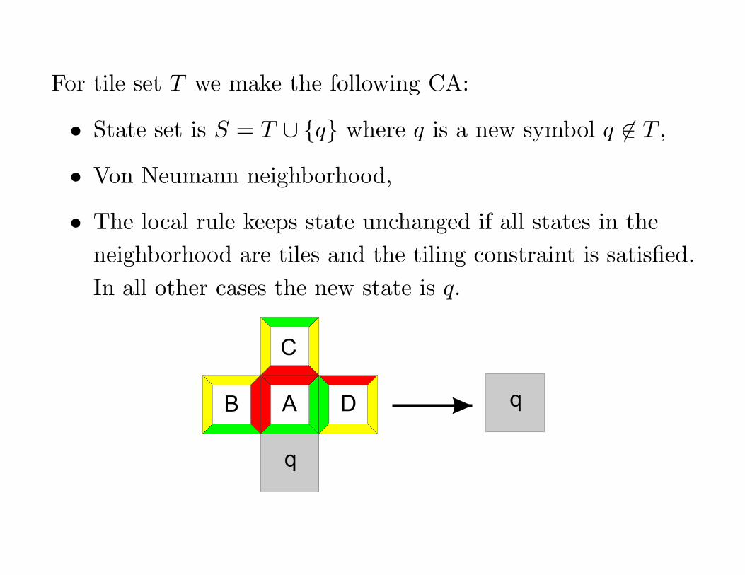
For tile set T we make the following CA:
• State set is S = T ∪ {q} where q is a new symbol q 6∈ T ,
B A
C
C
D A
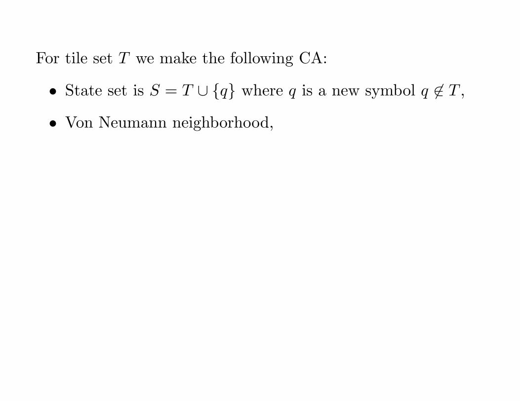
For tile set T we make the following CA:
• State set is S = T ∪ {q} where q is a new symbol q 6∈ T ,
• Von Neumann neighborhood,
B A
C
C
D A

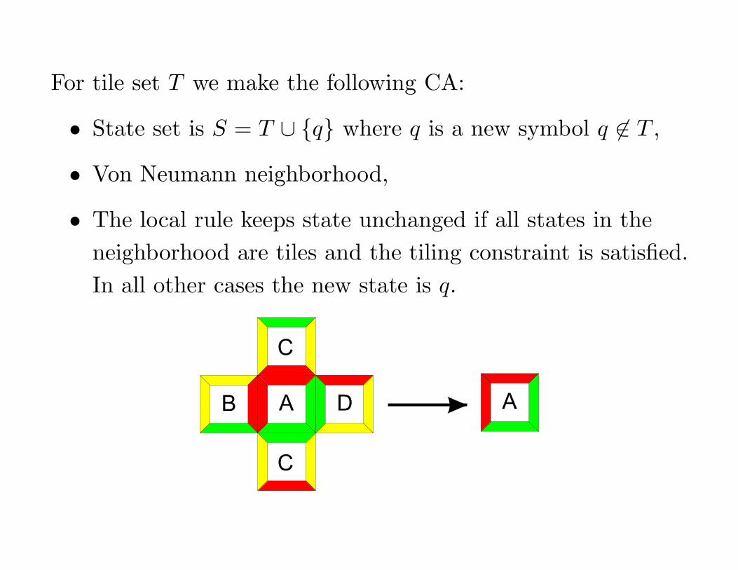
For tile set T we make the following CA:
• State set is S = T ∪ {q} where q is a new symbol q 6∈ T ,
• Von Neumann neighborhood,
• The local rule keeps state unchanged if all states in the
neighborhood are tiles and the tiling constraint is satisfied.
In all other cases the new state is q.
B A
C
C
D A
For tile set T we make the following CA:
• State set is S = T ∪ {q} where q is a new symbol q 6∈ T ,
• Von Neumann neighborhood,
• The local rule keeps state unchanged if all states in the
neighborhood are tiles and the tiling constraint is satisfied.
In all other cases the new state is q.
B A
C
D q
D
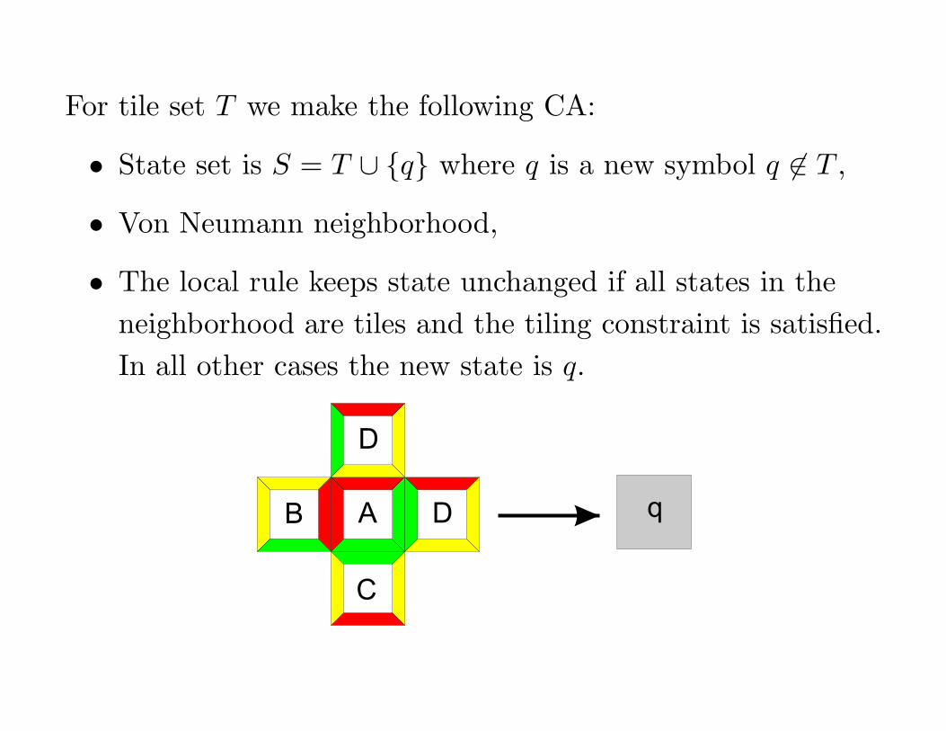
For tile set T we make the following CA:
• State set is S = T ∪ {q} where q is a new symbol q 6∈ T ,
• Von Neumann neighborhood,
• The local rule keeps state unchanged if all states in the
neighborhood are tiles and the tiling constraint is satisfied.
In all other cases the new state is q.
B A D q
C
q
For tile set T we make the following CA:
• State set is S = T ∪ {q} where q is a new symbol q 6∈ T ,
• Von Neumann neighborhood,
• The local rule keeps state unchanged if all states in the
neighborhood are tiles and the tiling constraint is satisfied.
In all other cases the new state is q.
For tile set T we make the following CA:
• State set is S = T ∪ {q} where q is a new symbol q 6∈ T ,
• Von Neumann neighborhood,
• The local rule keeps state unchanged if all states in the
neighborhood are tiles and the tiling constraint is satisfied.
In all other cases the new state is q.
=⇒ If T admits a tiling c then c is a non-quiescent fixed point
of the CA. So the CA is not nilpotent.
⇐= If T does not admit a valid tiling then every n × n square
contains a tiling error, for some n. State q propagates, so in at
most 2n steps all cells are in state q. The CA is nilpotent.
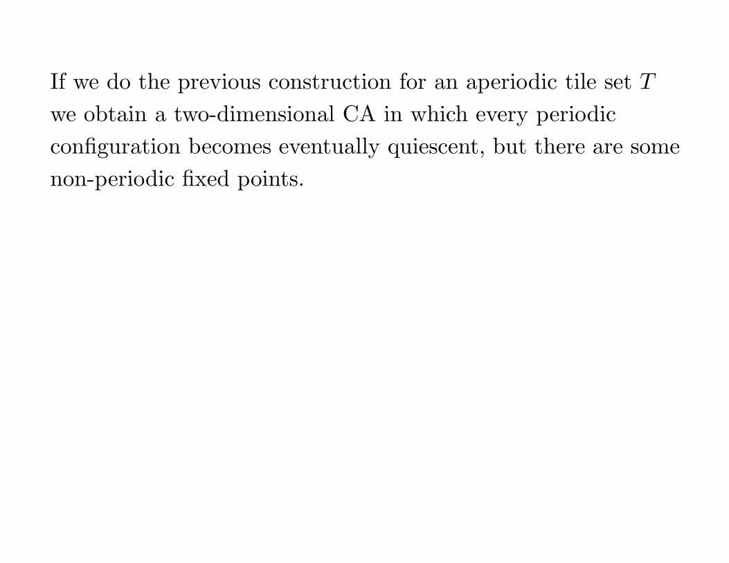
If we do the previous construction for an aperiodic tile set T
we obtain a two-dimensional CA in which every periodic
configuration becomes eventually quiescent, but there are some
non-periodic fixed points.
If we do the previous construction for an aperiodic tile set T
we obtain a two-dimensional CA in which every periodic
configuration becomes eventually quiescent, but there are some
non-periodic fixed points.
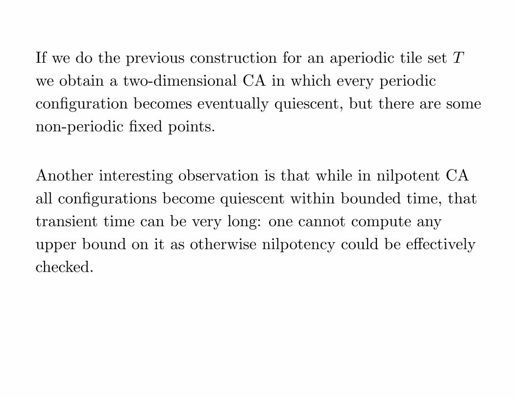
Another interesting observation is that while in nilpotent CA
all configurations become quiescent within bounded time, that
transient time can be very long: one cannot compute any
upper bound on it as otherwise nilpotency could be effectively
checked.
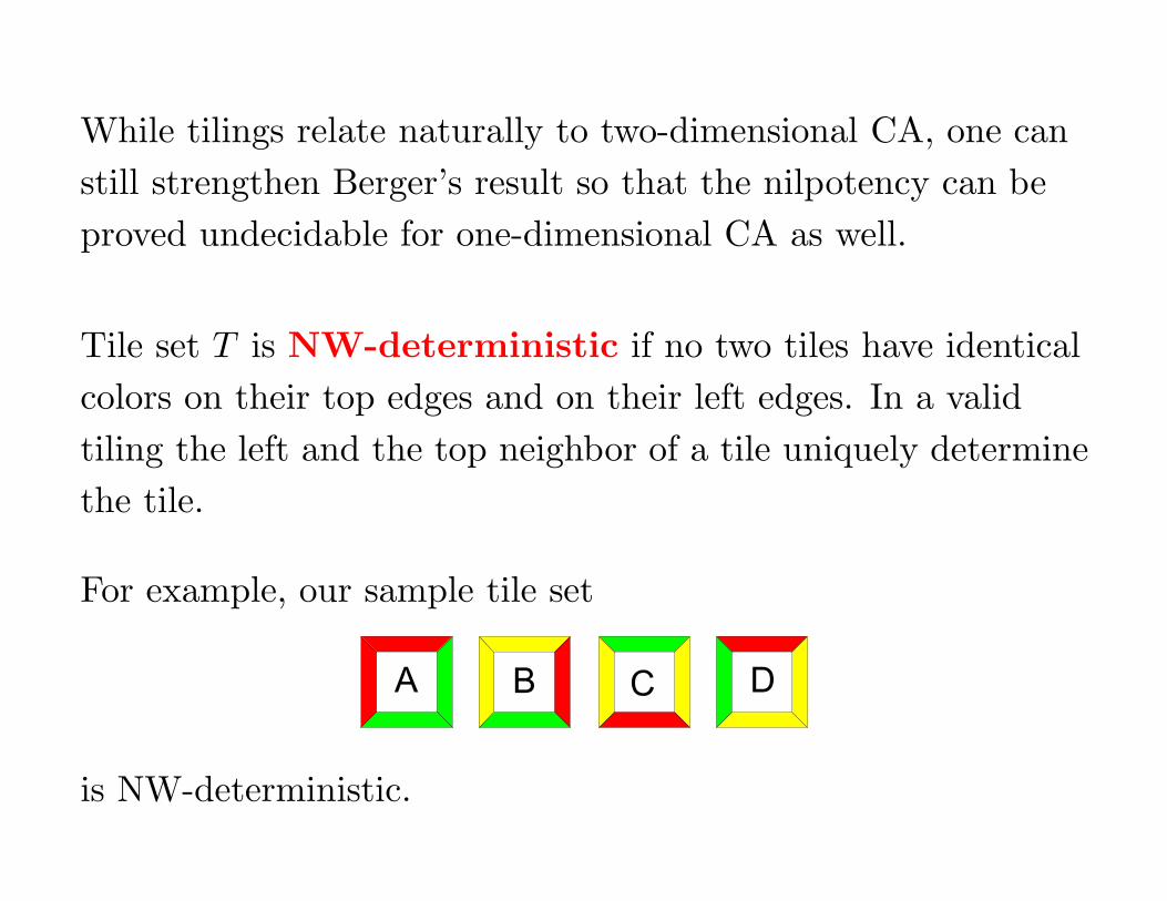
While tilings relate naturally to two-dimensional CA, one can
still strengthen Berger’s result so that the nilpotency can be
proved undecidable for one-dimensional CA as well.
Tile set T is NW-deterministic if no two tiles have identical
colors on their top edges and on their left edges. In a valid
tiling the left and the top neighbor of a tile uniquely determine
the tile.
For example, our sample tile set
A B C D
is NW-deterministic.
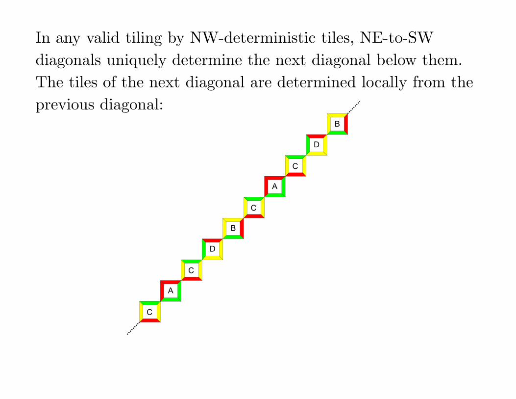
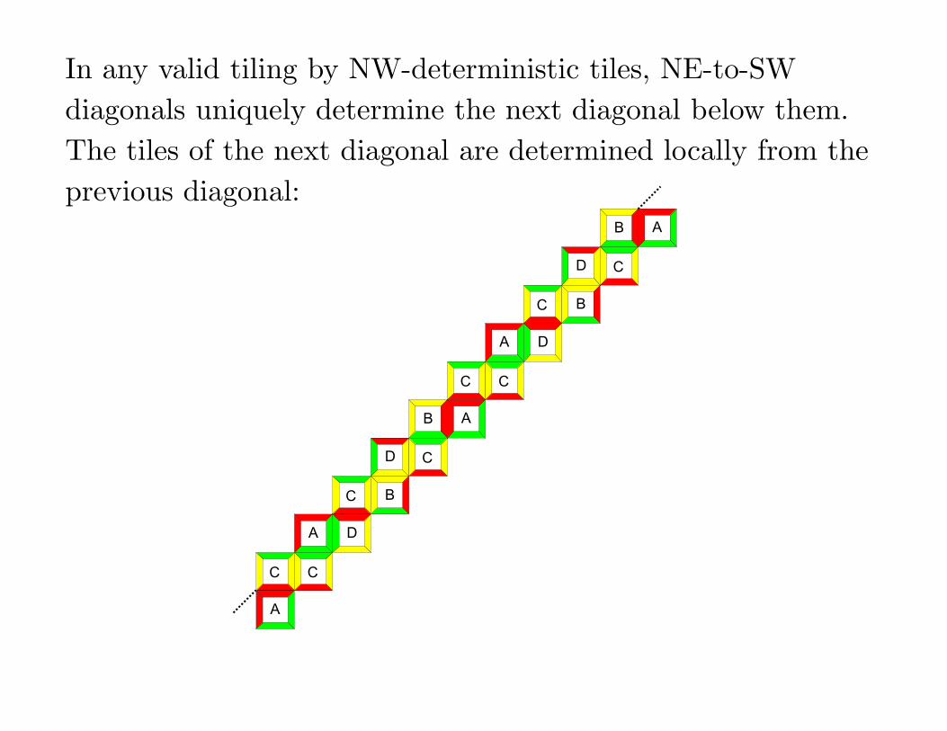
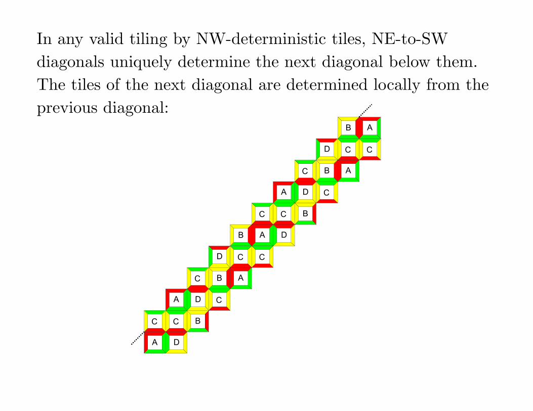
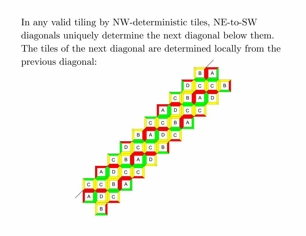
In any valid tiling by NW-deterministic tiles, NE-to-SW
diagonals uniquely determine the next diagonal below them.
The tiles of the next diagonal are determined locally from the
previous diagonal:
C
A
C
D
B
C
A
C
D
B
In any valid tiling by NW-deterministic tiles, NE-to-SW
diagonals uniquely determine the next diagonal below them.
The tiles of the next diagonal are determined locally from the
previous diagonal:
C
A
C
D
B
C
A
C
D
B
D
D
B
B
C
C
C
C
A
A
A
In any valid tiling by NW-deterministic tiles, NE-to-SW
diagonals uniquely determine the next diagonal below them.
The tiles of the next diagonal are determined locally from the
previous diagonal:
C
A
C
D
B
C
A
C
D
B
D
D
B
B
C
C
C
C
A
A
A D
D
B
C
A
C
B
C
A
C
In any valid tiling by NW-deterministic tiles, NE-to-SW
diagonals uniquely determine the next diagonal below them.
The tiles of the next diagonal are determined locally from the
previous diagonal:
C
A
C
D
B
C
A
C
D
B
D
D
B
B
C
C
C
C
A
A
A D
D
B
C
A
C
B
C
A
C
B
C
A
C
D
B
C
A
C
D
B
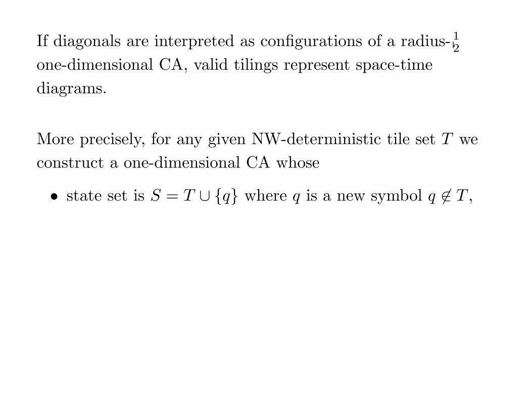
If diagonals are interpreted as configurations of a radius-12
one-dimensional CA, valid tilings represent space-time
diagrams.
ABC
If diagonals are interpreted as configurations of a radius-12
one-dimensional CA, valid tilings represent space-time
diagrams.
More precisely, for any given NW-deterministic tile set T we
construct a one-dimensional CA whose
• state set is S = T ∪ {q} where q is a new symbol q 6∈ T ,
ABC
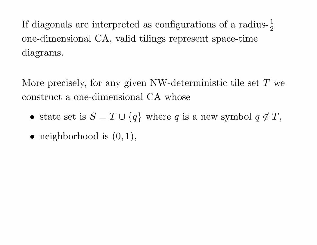
If diagonals are interpreted as configurations of a radius-12
one-dimensional CA, valid tilings represent space-time
diagrams.
More precisely, for any given NW-deterministic tile set T we
construct a one-dimensional CA whose
• state set is S = T ∪ {q} where q is a new symbol q 6∈ T ,
• neighborhood is (0, 1),
ABC
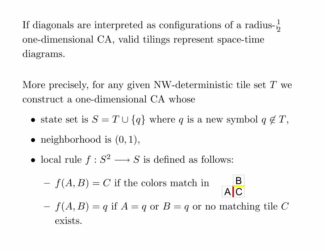
If diagonals are interpreted as configurations of a radius-12
one-dimensional CA, valid tilings represent space-time
diagrams.
More precisely, for any given NW-deterministic tile set T we
construct a one-dimensional CA whose
• state set is S = T ∪ {q} where q is a new symbol q 6∈ T ,
• neighborhood is (0, 1),
• local rule f : S2 −→ S is defined as follows:
– f(A,B) = C if the colors match inA
BC
– f(A,B) = q if A = q or B = q or no matching tile C
exists.
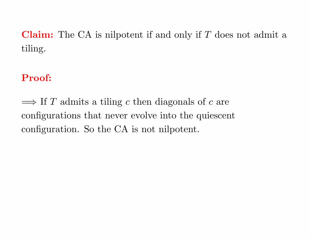
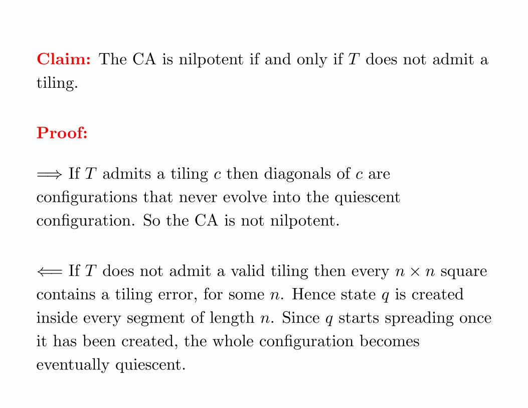
Claim: The CA is nilpotent if and only if T does not admit a
tiling.
Claim: The CA is nilpotent if and only if T does not admit a
tiling.
Proof:
=⇒ If T admits a tiling c then diagonals of c are
configurations that never evolve into the quiescent
configuration. So the CA is not nilpotent.
Claim: The CA is nilpotent if and only if T does not admit a
tiling.
Proof:
=⇒ If T admits a tiling c then diagonals of c are
configurations that never evolve into the quiescent
configuration. So the CA is not nilpotent.
⇐= If T does not admit a valid tiling then every n × n square
contains a tiling error, for some n. Hence state q is created
inside every segment of length n. Since q starts spreading once
it has been created, the whole configuration becomes
eventually quiescent.
Now we just need the following strengthening of Berger’s
theorem:
Theorem: The tiling problem is undecidable among
NW-deterministic tile sets.
and we have
Theorem: It is undecidable whether a given one-dimensional
CA (with spreading state q) is nilpotent.
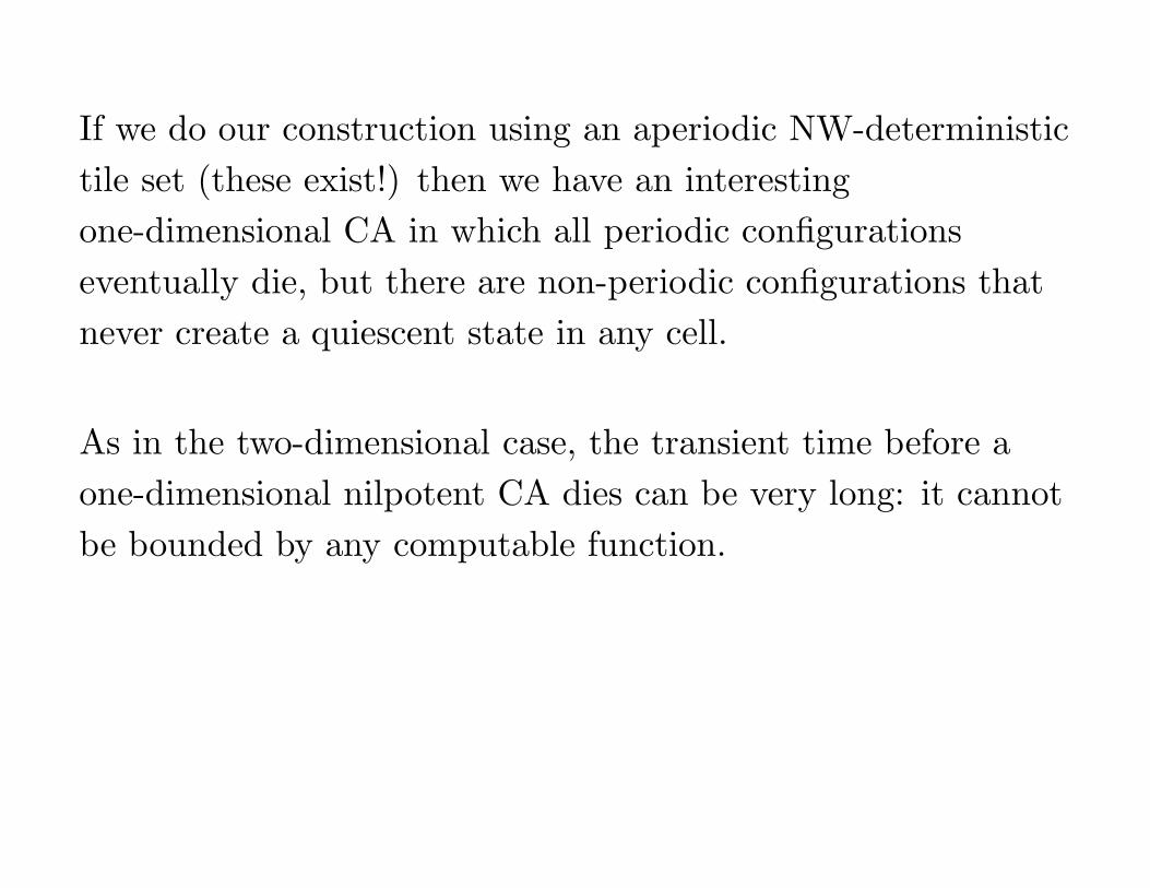
If we do our construction using an aperiodic NW-deterministic
tile set (these exist!) then we have an interesting
one-dimensional CA in which all periodic configurations
eventually die, but there are non-periodic configurations that
never create a quiescent state in any cell.
If we do our construction using an aperiodic NW-deterministic
tile set (these exist!) then we have an interesting
one-dimensional CA in which all periodic configurations
eventually die, but there are non-periodic configurations that
never create a quiescent state in any cell.
As in the two-dimensional case, the transient time before a
one-dimensional nilpotent CA dies can be very long: it cannot
be bounded by any computable function.

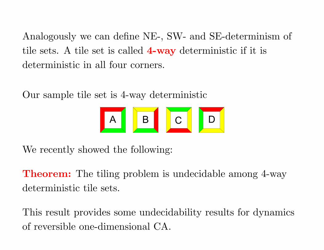
Analogously we can define NE-, SW- and SE-determinism of
tile sets. A tile set is called 4-way deterministic if it is
deterministic in all four corners.
Our sample tile set is 4-way deterministic
A B C D
Analogously we can define NE-, SW- and SE-determinism of
tile sets. A tile set is called 4-way deterministic if it is
deterministic in all four corners.
Our sample tile set is 4-way deterministic
A B C D
We recently showed the following:
Theorem: The tiling problem is undecidable among 4-way
deterministic tile sets.
This result provides some undecidability results for dynamics
of reversible one-dimensional CA.
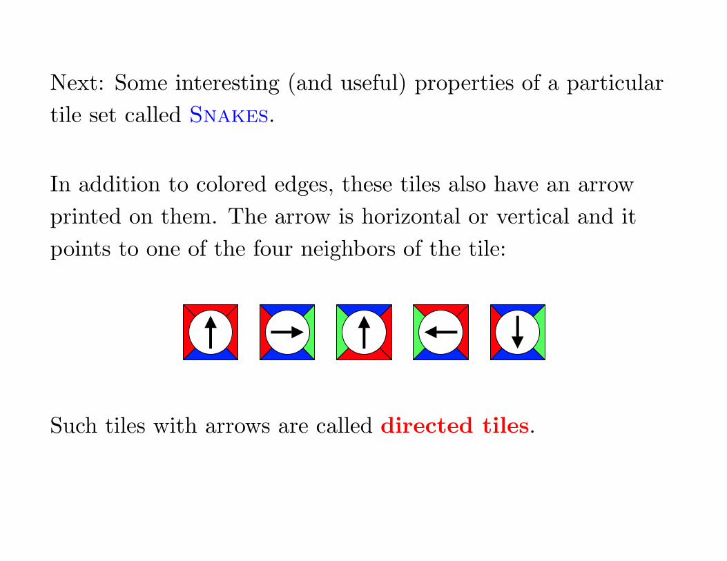
Next: Some interesting (and useful) properties of a particular
tile set called Snakes.
In addition to colored edges, these tiles also have an arrow
printed on them. The arrow is horizontal or vertical and it
points to one of the four neighbors of the tile:
Such tiles with arrows are called directed tiles.
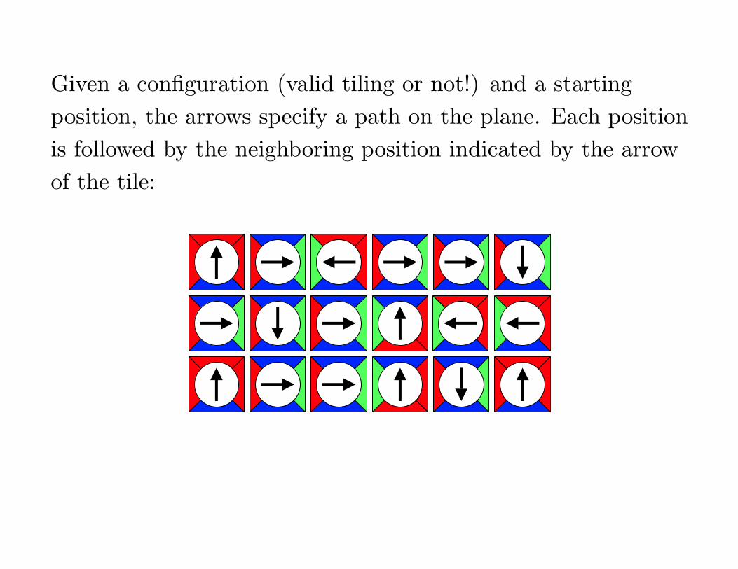
Given a configuration (valid tiling or not!) and a starting
position, the arrows specify a path on the plane. Each position
is followed by the neighboring position indicated by the arrow
of the tile:
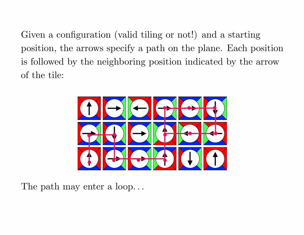
Given a configuration (valid tiling or not!) and a starting
position, the arrows specify a path on the plane. Each position
is followed by the neighboring position indicated by the arrow
of the tile:
The path may enter a loop. . .
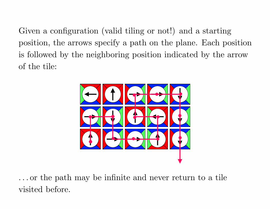
Given a configuration (valid tiling or not!) and a starting
position, the arrows specify a path on the plane. Each position
is followed by the neighboring position indicated by the arrow
of the tile:
. . . or the path may be infinite and never return to a tile
visited before.
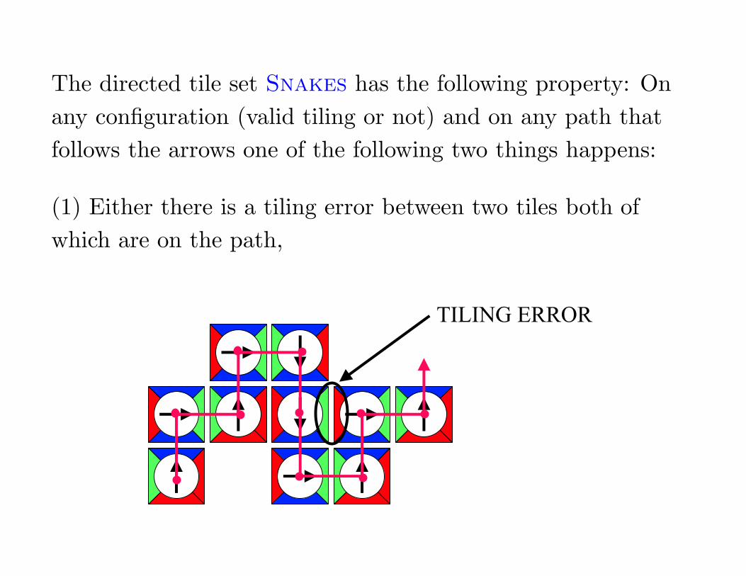
The directed tile set Snakes has the following property: On
any configuration (valid tiling or not) and on any path that
follows the arrows one of the following two things happens:
(1) Either there is a tiling error between two tiles both of
which are on the path,
TILING ERROR
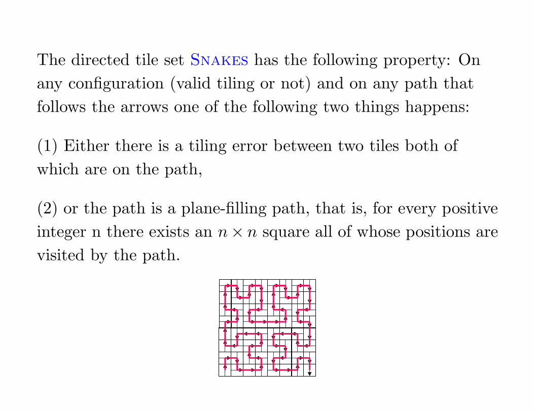
The directed tile set Snakes has the following property: On
any configuration (valid tiling or not) and on any path that
follows the arrows one of the following two things happens:
(1) Either there is a tiling error between two tiles both of
which are on the path,
(2) or the path is a plane-filling path, that is, for every positive
integer n there exists an n× n square all of whose positions are
visited by the path.
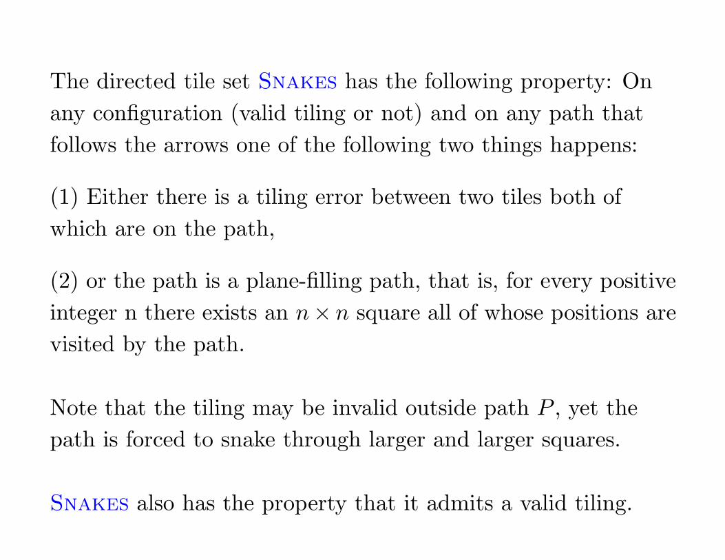
Note that the tiling may be invalid outside path P , yet the
path is forced to snake through larger and larger squares.
Snakes also has the property that it admits a valid tiling.
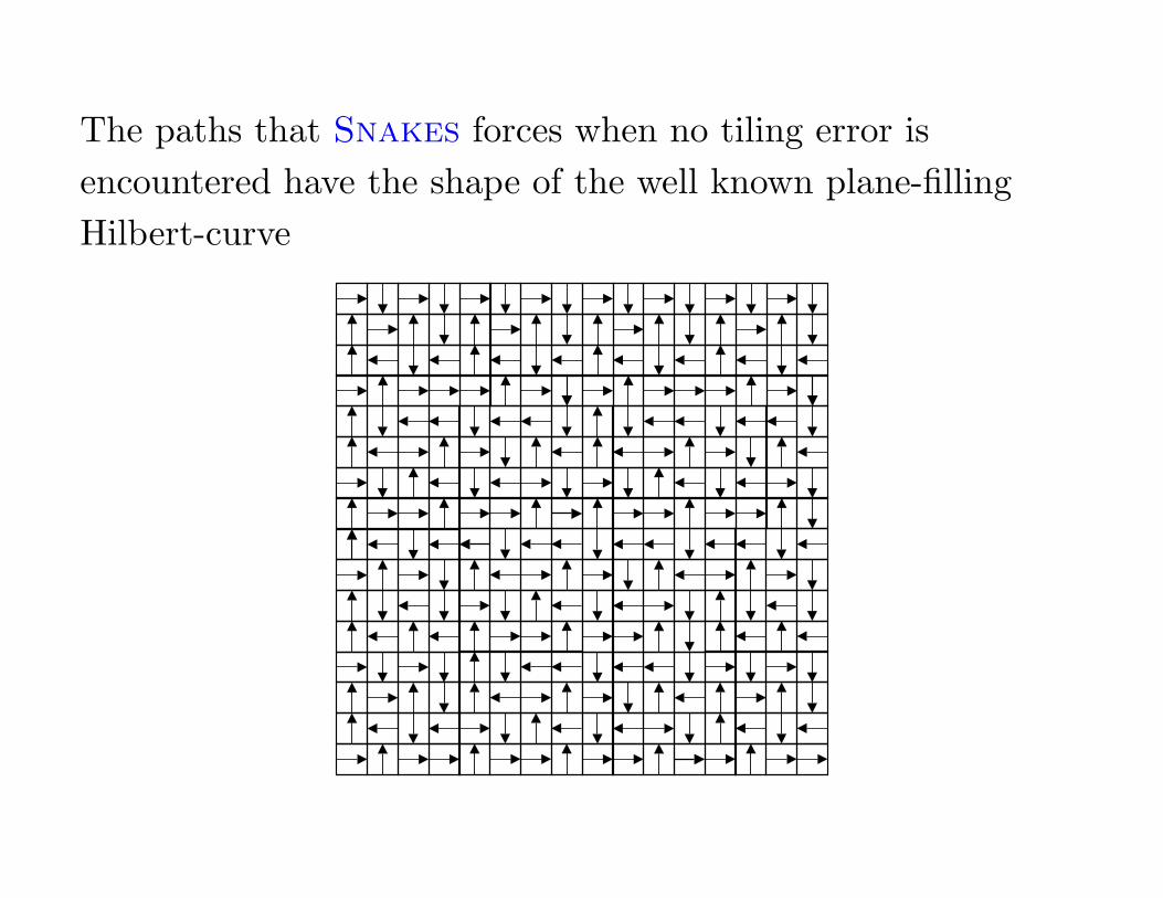
The paths that Snakes forces when no tiling error is
encountered have the shape of the well known plane-filling
Hilbert-curve
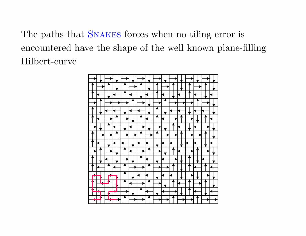
The paths that Snakes forces when no tiling error is
encountered have the shape of the well known plane-filling
Hilbert-curve
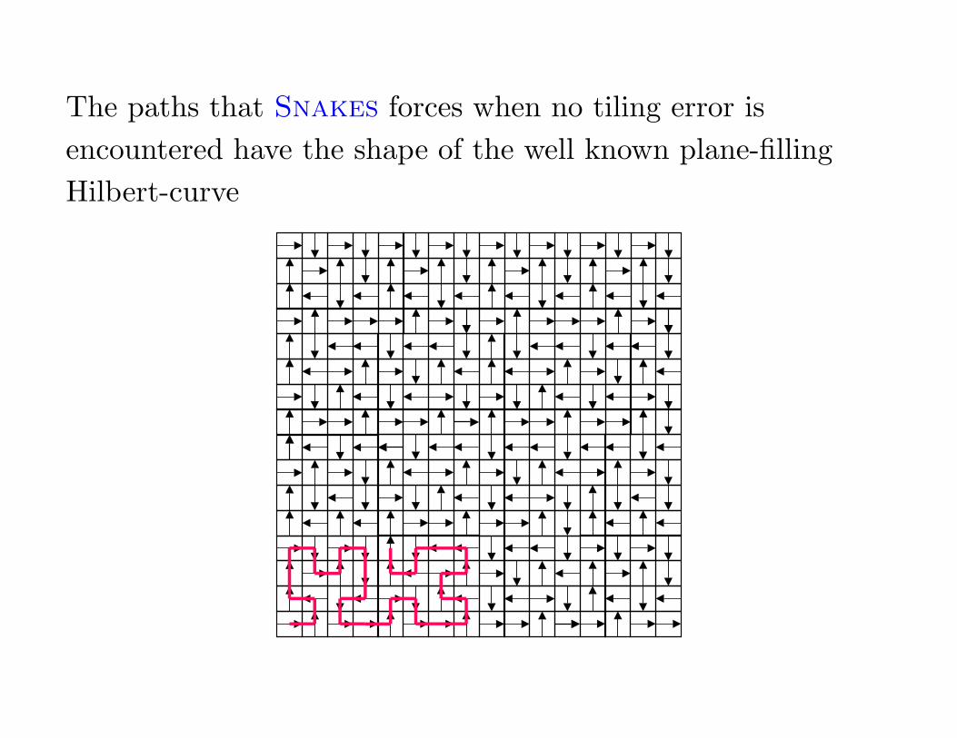
The paths that Snakes forces when no tiling error is
encountered have the shape of the well known plane-filling
Hilbert-curve
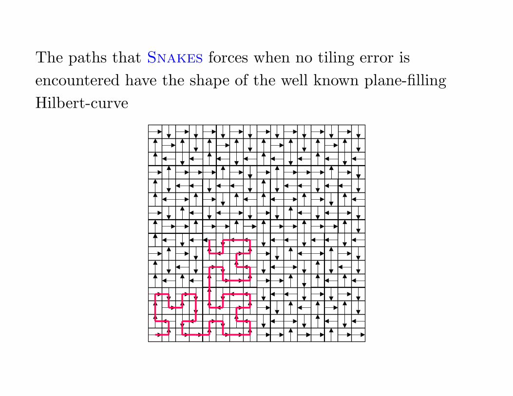
The paths that Snakes forces when no tiling error is
encountered have the shape of the well known plane-filling
Hilbert-curve
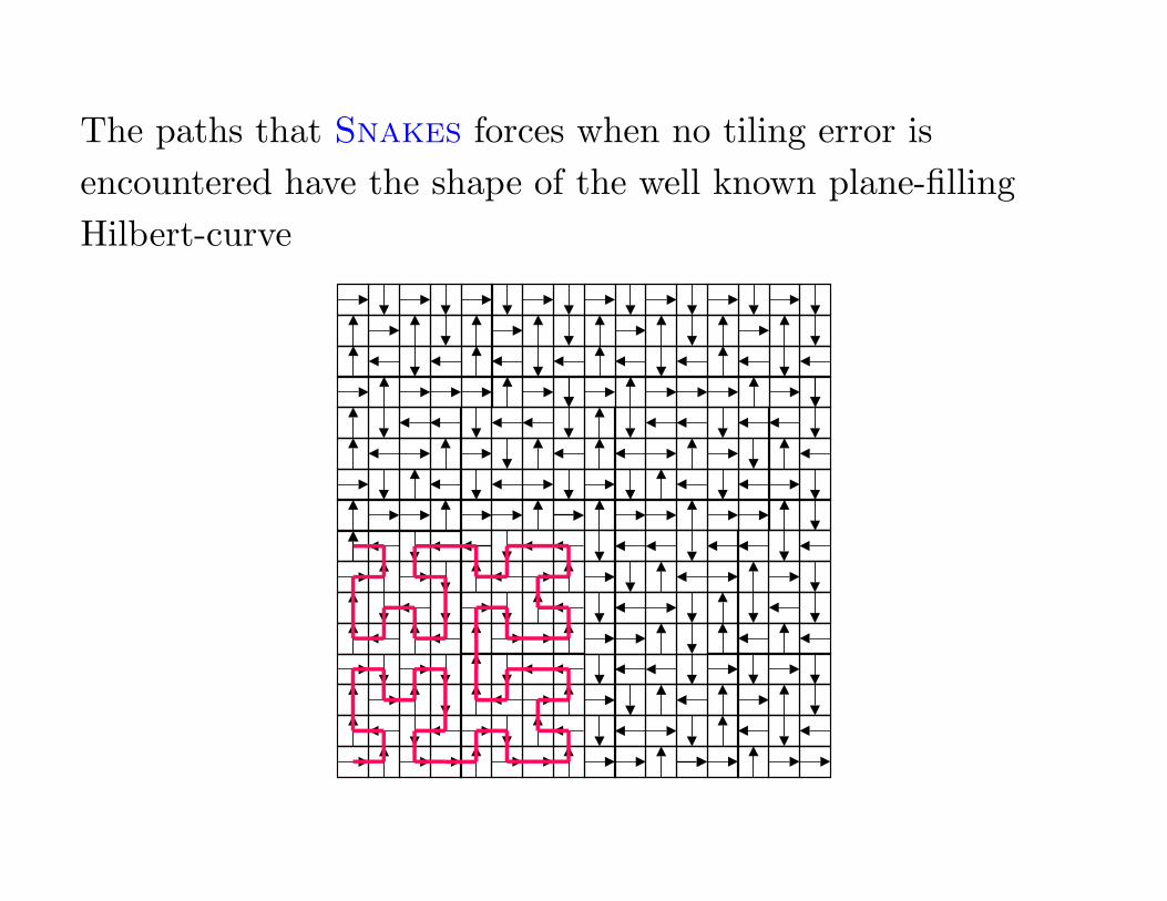
The paths that Snakes forces when no tiling error is
encountered have the shape of the well known plane-filling
Hilbert-curve
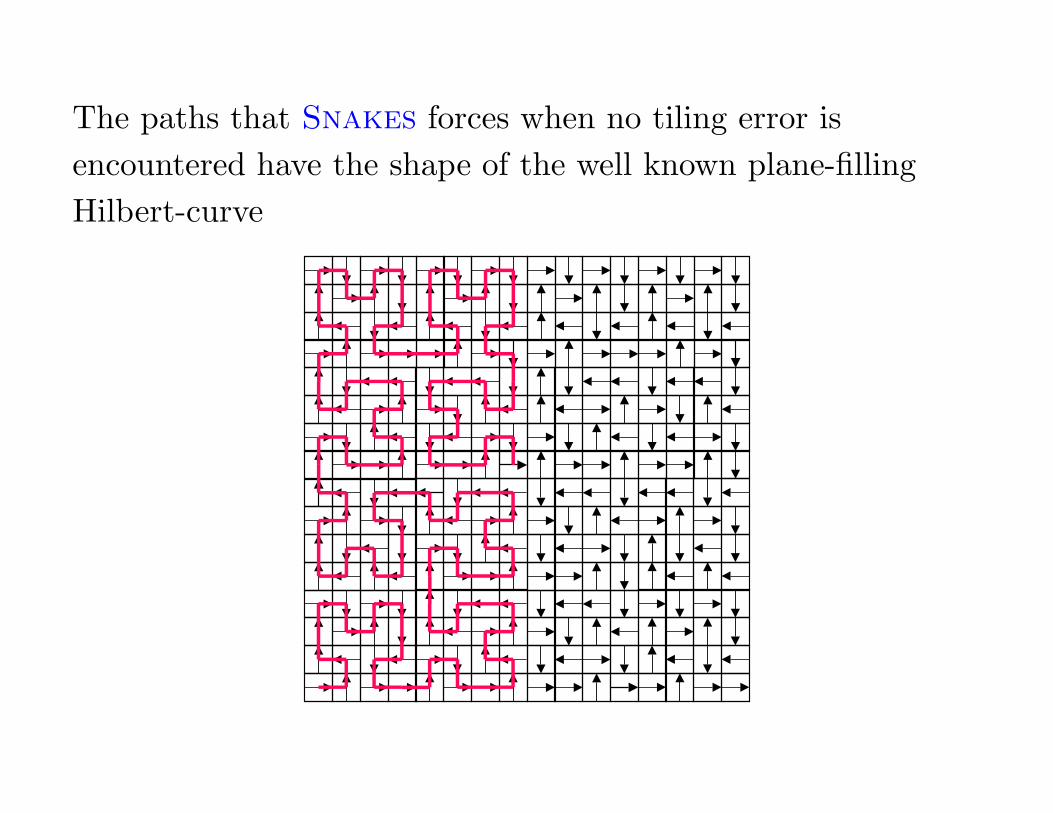
The paths that Snakes forces when no tiling error is
encountered have the shape of the well known plane-filling
Hilbert-curve
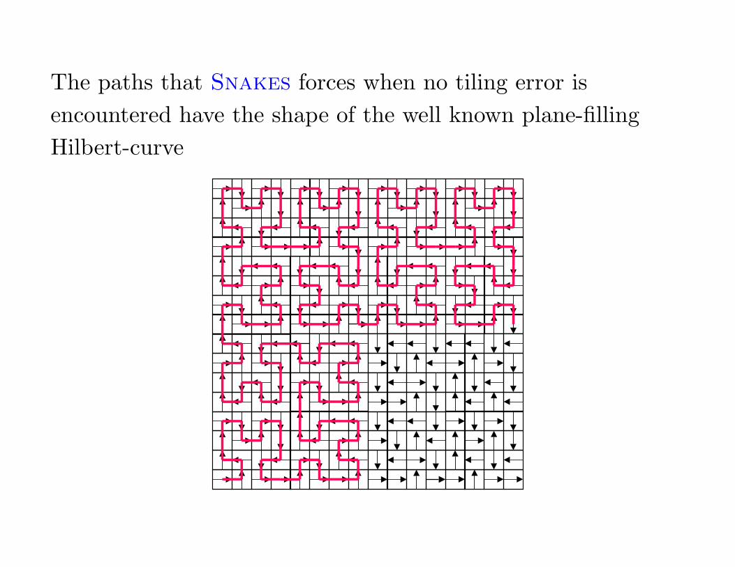
The paths that Snakes forces when no tiling error is
encountered have the shape of the well known plane-filling
Hilbert-curve
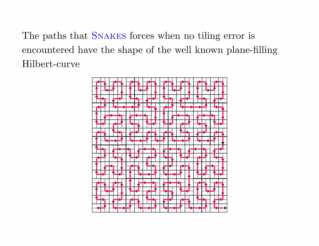
The paths that Snakes forces when no tiling error is
encountered have the shape of the well known plane-filling
Hilbert-curve
First application of Snakes: An example of a two-dimensional
CA that is injective on periodic configurations but is not
injective on all configurations.
First application of Snakes: An example of a two-dimensional
CA that is injective on periodic configurations but is not
injective on all configurations.
Let GP denote the restriction of CA function G into periodic
configurations.
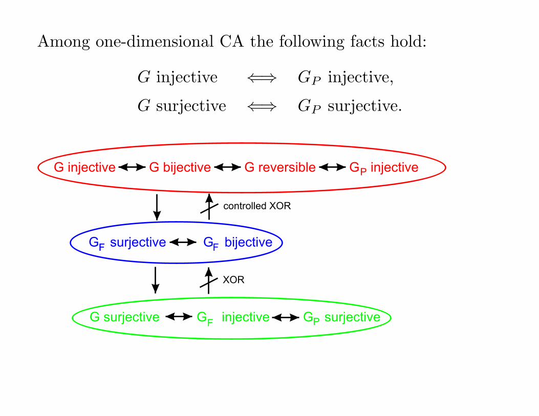
Among one-dimensional CA the following facts hold:
G injective ⇐⇒ GP injective,
G surjective ⇐⇒ GP surjective.
G injective G bijective G reversible G injective
G surjective G bijective
G surjective G injective G surjective
F
F
F F
XOR
controlled XOR
P
P
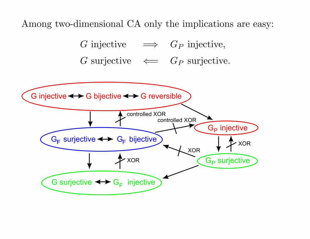
Among two-dimensional CA only the implications are easy:
G injective =⇒ GP injective,
G surjective ⇐= GP surjective.
G injective G bijective G reversible
G surjective G bijective
G surjective G injective
F
F
F F
XOR
controlled XOR
P
PG injective
G surjective
XOR
XOR
controlled XOR
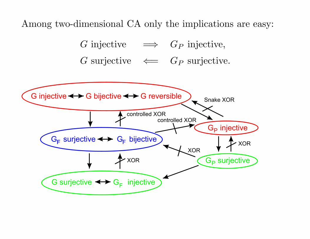
Among two-dimensional CA only the implications are easy:
G injective =⇒ GP injective,
G surjective ⇐= GP surjective.
G injective G bijective G reversible
G surjective G bijective
G surjective G injective
F
F
F F
XOR
controlled XOR
P
PG injective
G surjective
XOR
XOR
controlled XOR
Snake XOR
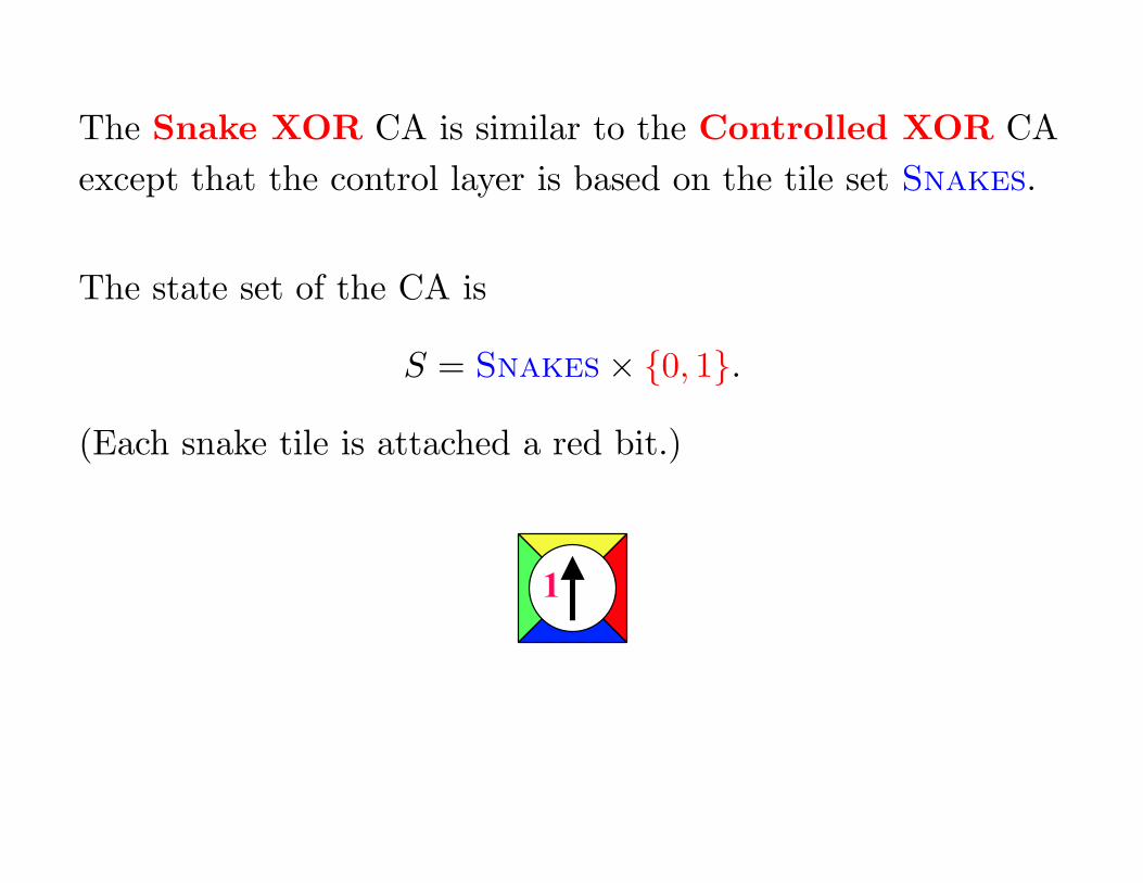
The Snake XOR CA is similar to the Controlled XOR CA
except that the control layer is based on the tile set Snakes.
The state set of the CA is
S = Snakes × {0, 1}.
(Each snake tile is attached a red bit.)
1
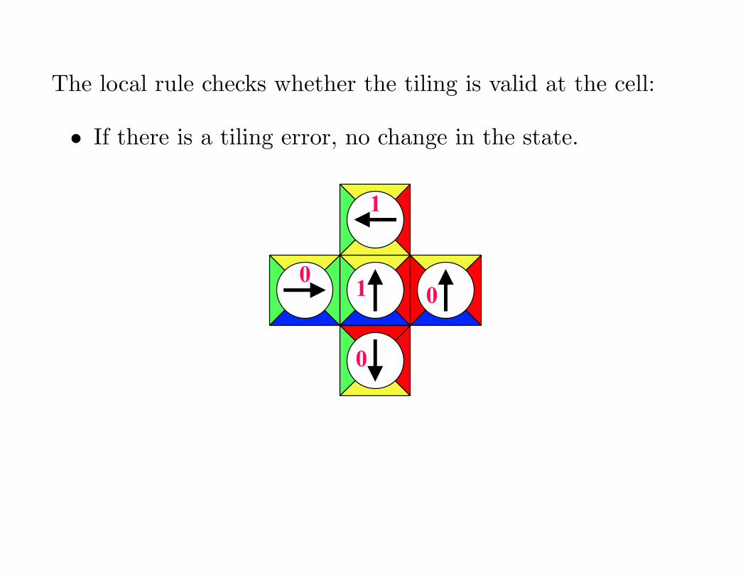
The local rule checks whether the tiling is valid at the cell:
• If there is a tiling error, no change in the state.
0
0
01
1

The local rule checks whether the tiling is valid at the cell:
• If there is a tiling error, no change in the state.
• If the tiling is valid, XOR rule is applied with the neighbor
pointed to by the arrow on the tile.
0
0
01
1
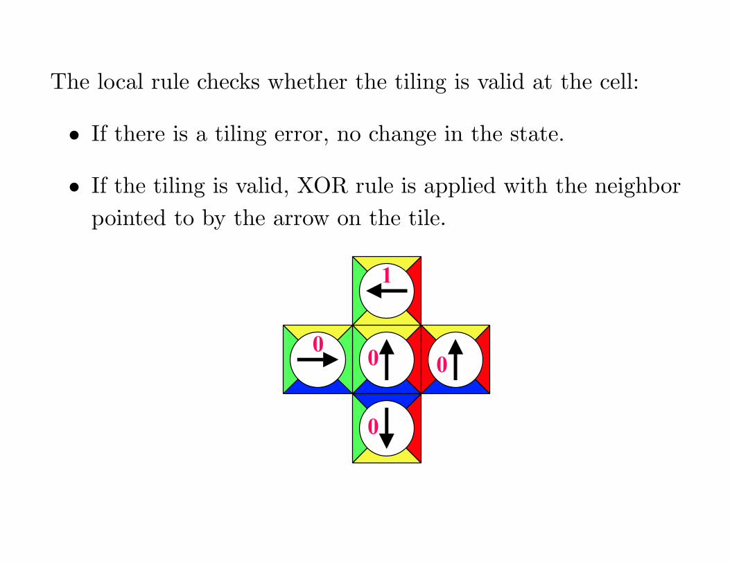
The local rule checks whether the tiling is valid at the cell:
• If there is a tiling error, no change in the state.
• If the tiling is valid, XOR rule is applied with the neighbor
pointed to by the arrow on the tile.
0
0
00
1
Snake XOR is not injective:
The following two configurations have the same successor: The
Snakes tilings of the configurations form the same valid tiling
of the plane. In one of the configurations all bits are set to 0,
and in the other configuration all bits are 1.
All cells are active because the tilings are correct. This means
that all bits in both configurations become 0. So the two
configurations become identical. The CA is not injective.
Snake XOR is injective on periodic configurations:
Suppose there are different periodic configurations c and d
with the same successor. Since only bits may change, c and d
must have identical Snakes tiles everywhere. So they must
have different bits 0 and 1 in some position ~p1 ∈ Z2.
Snake XOR is injective on periodic configurations:
Suppose there are different periodic configurations c and d
with the same successor. Since only bits may change, c and d
must have identical Snakes tiles everywhere. So they must
have different bits 0 and 1 in some position ~p1 ∈ Z2.
Because c and d have identical successors, the cell in position
~p1 must be active, that is, the Snakes tiling is valid in
position ~p1. Moreover, the bits stored in the neighboring
position ~p2 (pointed by the arrow) are different in c and d.
Hence we can repeat the reasoning in position ~p2.
The same reasoning can be repeated over and over again. The
positions ~p1, ~p2, ~p3, . . . form a path that follows the arrows on
the tiles. There is no tiling error at any tile on this path.
But this contradicts the fact that the plane filling property of
Snakes guarantees that on periodic tiling every path
encounters a tiling error.
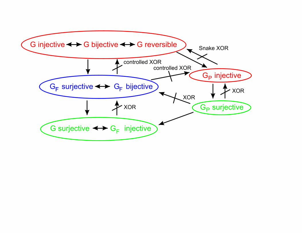
G injective G bijective G reversible
G surjective G bijective
G surjective G injective
F
F
F F
XOR
controlled XOR
P
PG injective
G surjective
XOR
XOR
controlled XOR
Snake XOR
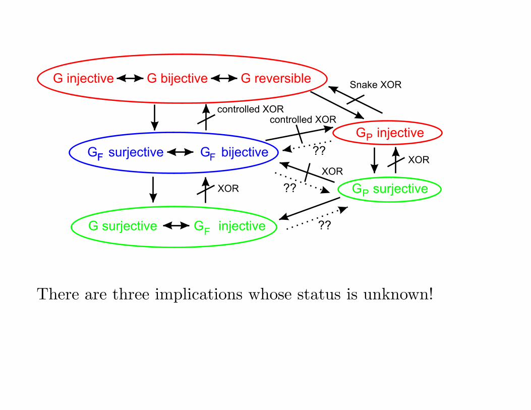
G injective G bijective G reversible
G surjective G bijective
G surjective G injective
F
F
F F
XOR
controlled XOR
P
PG injective
G surjective
XOR
XOR
controlled XOR
??
??
??
Snake XOR
There are three implications whose status is unknown!
Second application of Snakes: It is undecidable to determine
if a given two-dimensional CA is reversible.
Snakes
T
0/1
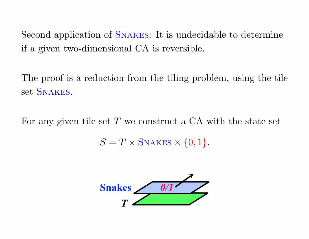
Second application of Snakes: It is undecidable to determine
if a given two-dimensional CA is reversible.
The proof is a reduction from the tiling problem, using the tile
set Snakes.
For any given tile set T we construct a CA with the state set
S = T × Snakes × {0, 1}.
Snakes
T
0/1
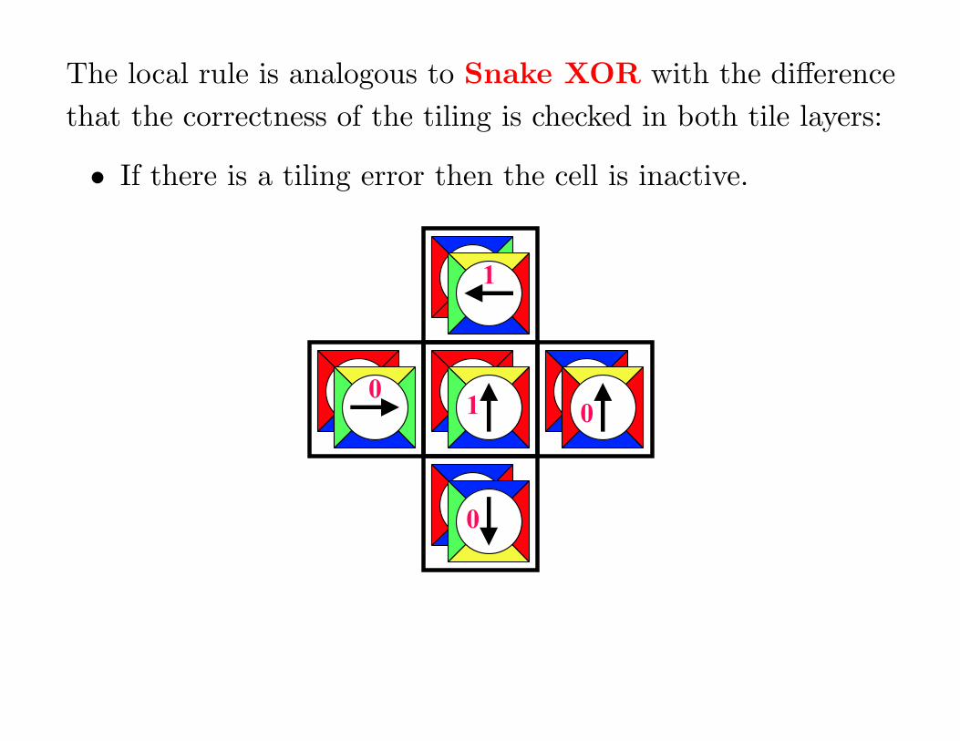
The local rule is analogous to Snake XOR with the difference
that the correctness of the tiling is checked in both tile layers:
• If there is a tiling error then the cell is inactive.
0
0
01
1
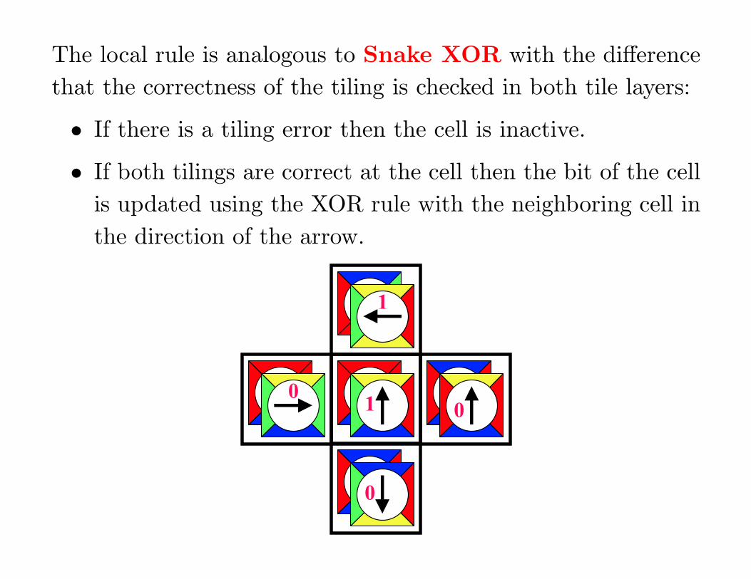
The local rule is analogous to Snake XOR with the difference
that the correctness of the tiling is checked in both tile layers:
• If there is a tiling error then the cell is inactive.
• If both tilings are correct at the cell then the bit of the cell
is updated using the XOR rule with the neighboring cell in
the direction of the arrow.
0
0
01
1
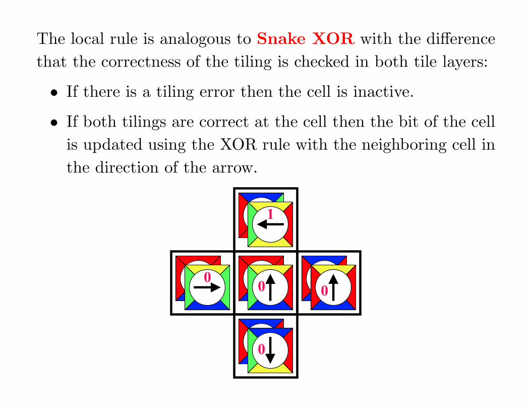
The local rule is analogous to Snake XOR with the difference
that the correctness of the tiling is checked in both tile layers:
• If there is a tiling error then the cell is inactive.
• If both tilings are correct at the cell then the bit of the cell
is updated using the XOR rule with the neighboring cell in
the direction of the arrow.
0
0
00
1
We can reason exactly as with Smake XOR, and show that
the CA is reversible if and only if the tile set T does not admit
a plane tiling:
We can reason exactly as with Smake XOR, and show that
the CA is reversible if and only if the tile set T does not admit
a plane tiling:
(=⇒) If a valid tiling of the plane exists then we can construct
two different configurations of the CA that have the same
image under G. The Snakes and the T layers of the
configurations form the same valid tilings of the plane. In one
of the configurations all bits are 0, and in the other
configuration all bits are 1.
All cells are active because the tilings are correct. This means
that all bits in both configurations become 0. So the two
configurations become identical. The CA is not injective.
(⇐=) Conversely, assume that the CA is not injective. Let c
and d be two different configurations with the same successor.
Since only bits may change, c and d must have identical
Snakes and T layers. So they must have different bits 0 and 1
in some position ~p1 ∈ Z2.
(⇐=) Conversely, assume that the CA is not injective. Let c
and d be two different configurations with the same successor.
Since only bits may change, c and d must have identical
Snakes and T layers. So they must have different bits 0 and 1
in some position ~p1 ∈ Z2.
Because c and d have identical successors, the cell in position
~p1 must be active, that is, the tilings with both tile components
are valid in position ~p1. Moreover, the bits stored in the
neighboring position ~p2 (pointed by the arrow) are different in
c and d. Hence we can repeat the reasoning in position ~p2.
The same reasoning can be repeated over and over again. The
positions ~p1, ~p2, ~p3, . . . form a path that follows the arrows on
the tiles. There is no tiling error at any tile on this path so the
special property of Snakes forces the path to cover arbitrarily
large squares.
Hence T admits tilings of arbitrarily large squares, and
consequently a tiling of the infinite plane.
Theorem: It is undecidable whether a given two-dimensional
CA is injective.
An analogous (but simpler!) construction can be made for the
surjectivity problem, based on the fact surjectivity is
equivalent to injectivity on finite configurations:
Theorem: It is undecidable whether a given two-dimensional
CA is surjective.
Both problems are semi-decidable in one direction:
Injectivity is semi-decidable: Enumerate all CA G one-by
one and check if G is the inverse of the given CA. Halt once (if
ever) the inverse is found.
Non-surjectivity is semi-decidable: Enumerate all finite
patterns one-by-one and halt once (if ever) an orphan is found.
From the undecidability of injectivity we obtain the interesting
fact that there are some reversible CA that use von Neumann
neighborhood but whose inverse automata use a very large
neighborhood: There can be no computable upper bound on
the extend of this inverse neighborhood.
So while topological arguments show that a finite
neighborhood is enough to determine the previous state of a
cell, computation theory shows that this neighborhood may be
extremely large.
From the undecidability of surjectivity we see that that there
are non-surjective CA whose smallest orphan is very large:
There can be no computable upper bound on the extend of the
smallest orphan.
So while the smallest known orphan for Game-Of-Life is pretty
big (113 cells), this pales in comparison with some other CA.
Both reversibility and surjectivity can be easily decided among
one-dimensional CA:
Theorem (Amoroso, Patt 1972): It is decidable whether a
given one-dimensional CA is injective (or surjective).
Both reversibility and surjectivity can be easily decided among
one-dimensional CA:
Theorem (Amoroso, Patt 1972): It is decidable whether a
given one-dimensional CA is injective (or surjective).
We also know the tight bound on the extend of the inverse
neighborhood: The neighborhood of a radius-12 injective CA
with n states consists of at most n − 1 consecutive cells.
We do not know any polynomial upper bound on the length of
the smallest orphan for a radius- 12 non-surjective CA with n
states.
A CA G is called periodic if all configurations are temporally
periodic. In this case there is a positive integer n such that Gn
is the identity function.
The CA we constructed in the undecidability proof for
reversibility is periodic when reversible. Hence we have
Theorem: It is undecidable whether a given two-dimensional
CA is periodic.
Recently (in 2008) with N.Ollinger we showed that periodicity
is also undecidable among one-dimensional CA:
Theorem: It is undecidable whether a given one-dimensional
CA is periodic.
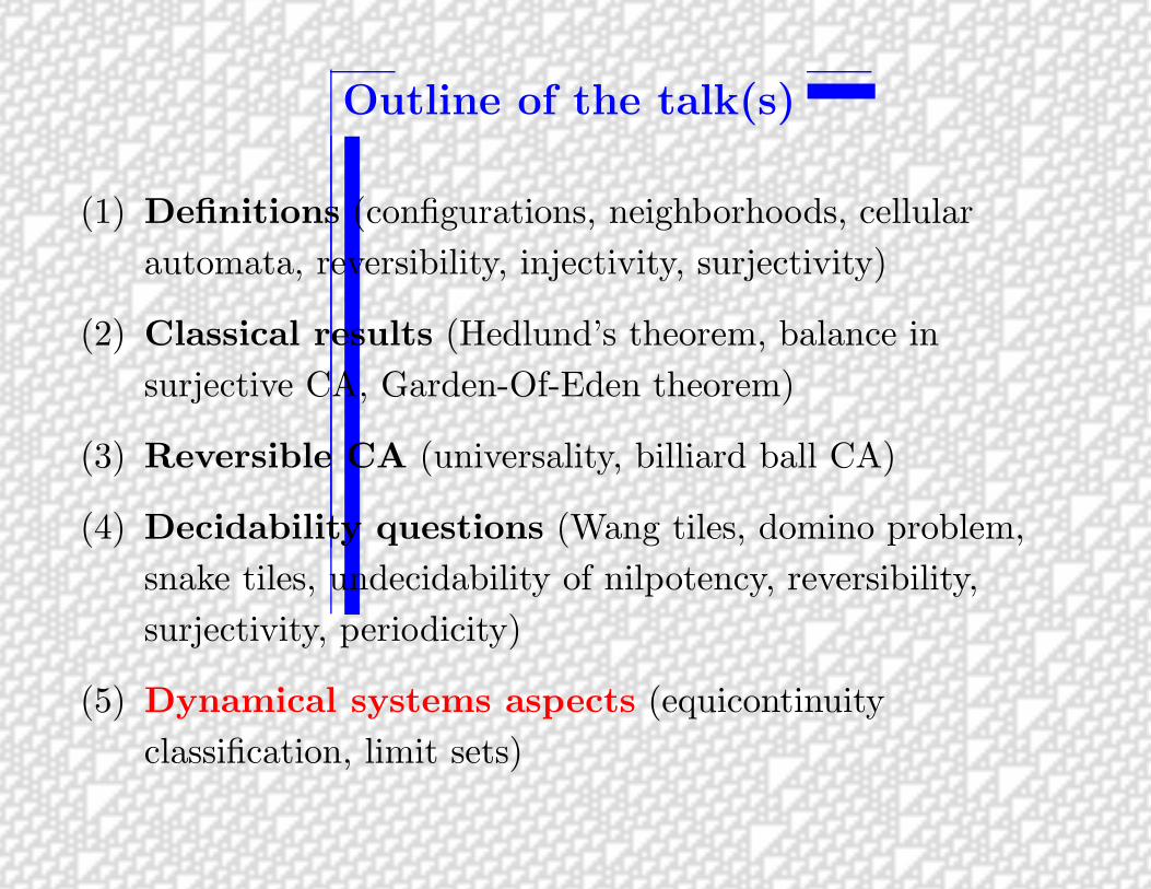
Outline of the talk(s)
(1) Definitions (configurations, neighborhoods, cellular
automata, reversibility, injectivity, surjectivity)
(2) Classical results (Hedlund’s theorem, balance in
surjective CA, Garden-Of-Eden theorem)
(3) Reversible CA (universality, billiard ball CA)
(4) Decidability questions (Wang tiles, domino problem,
snake tiles, undecidability of nilpotency, reversibility,
surjectivity, periodicity)
(5) Dynamical systems aspects (equicontinuity
classification, limit sets)
A topological dynamical system is a pair (X,F ) where X is a
compact space and F : X −→ X is continuous. We know that
(SZd
, G) is such a dynamical system, so concepts and methods
of topological dynamics can be applied to cellular automata.
In the study of chaotic behavior one is interested in the
propagation of errors during iterations of the system. This is
also relevant to simulations by cellular automata: iterations of
the CA inside a finite window may not give a reliable picture if
the system is sensitive to changes in states outside the
observation window.
The results reported here are proved for one-dimensional CA.
Nevertheless, the concepts can be defined for any
dimensionality d.
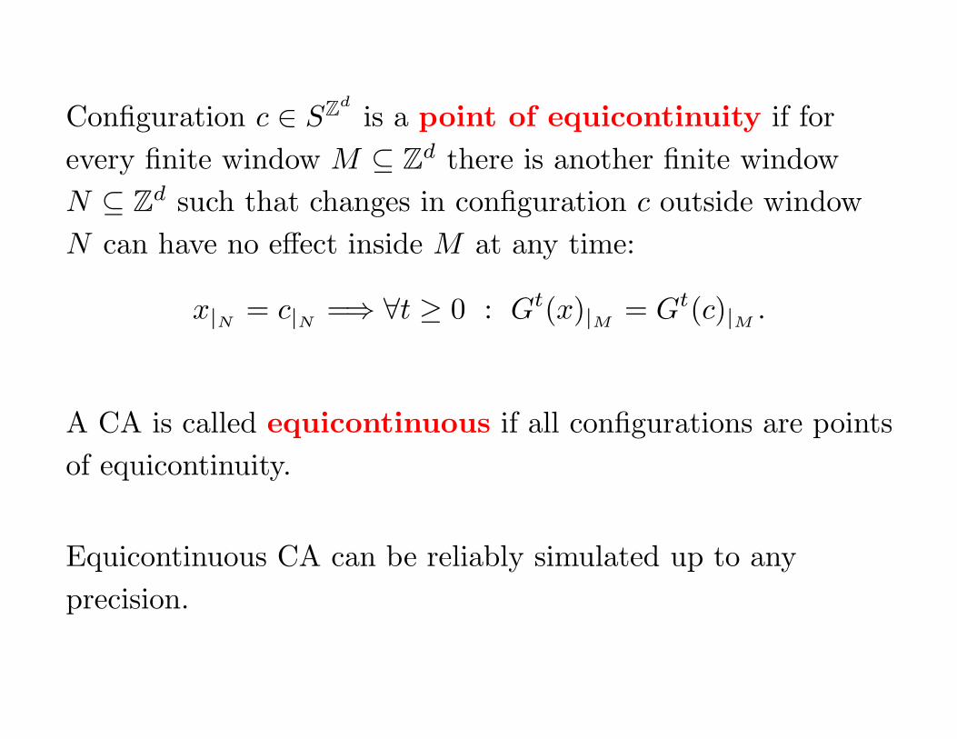
Configuration c ∈ SZd
is a point of equicontinuity if for
every finite window M ⊆ Zd there is another finite window
N ⊆ Zd such that changes in configuration c outside window
N can have no effect inside M at any time:
x|N = c|N =⇒ ∀t ≥ 0 : Gt(x)|M = Gt(c)|M .
A CA is called equicontinuous if all configurations are points
of equicontinuity.
Equicontinuous CA can be reliably simulated up to any
precision.
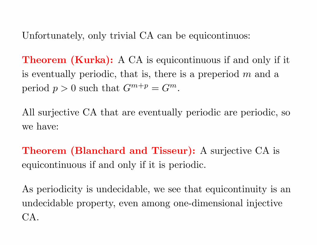
Unfortunately, only trivial CA can be equicontinuos:
Theorem (Kurka): A CA is equicontinuous if and only if it
is eventually periodic, that is, there is a preperiod m and a
period p > 0 such that Gm+p = Gm.
All surjective CA that are eventually periodic are periodic, so
we have:
Theorem (Blanchard and Tisseur): A surjective CA is
equicontinuous if and only if it is periodic.
As periodicity is undecidable, we see that equicontinuity is an
undecidable property, even among one-dimensional injective
CA.
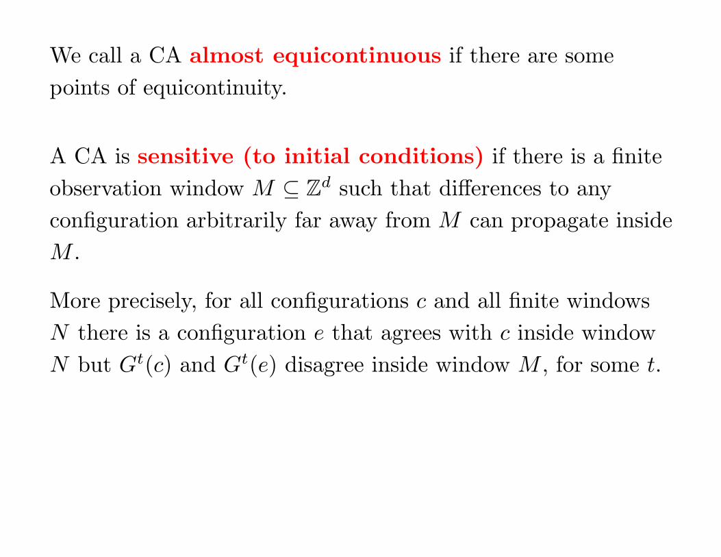
We call a CA almost equicontinuous if there are some
points of equicontinuity.
A CA is sensitive (to initial conditions) if there is a finite
observation window M ⊆ Zd such that differences to any
configuration arbitrarily far away from M can propagate inside
M .
More precisely, for all configurations c and all finite windows
N there is a configuration e that agrees with c inside window
N but Gt(c) and Gt(e) disagree inside window M , for some t.
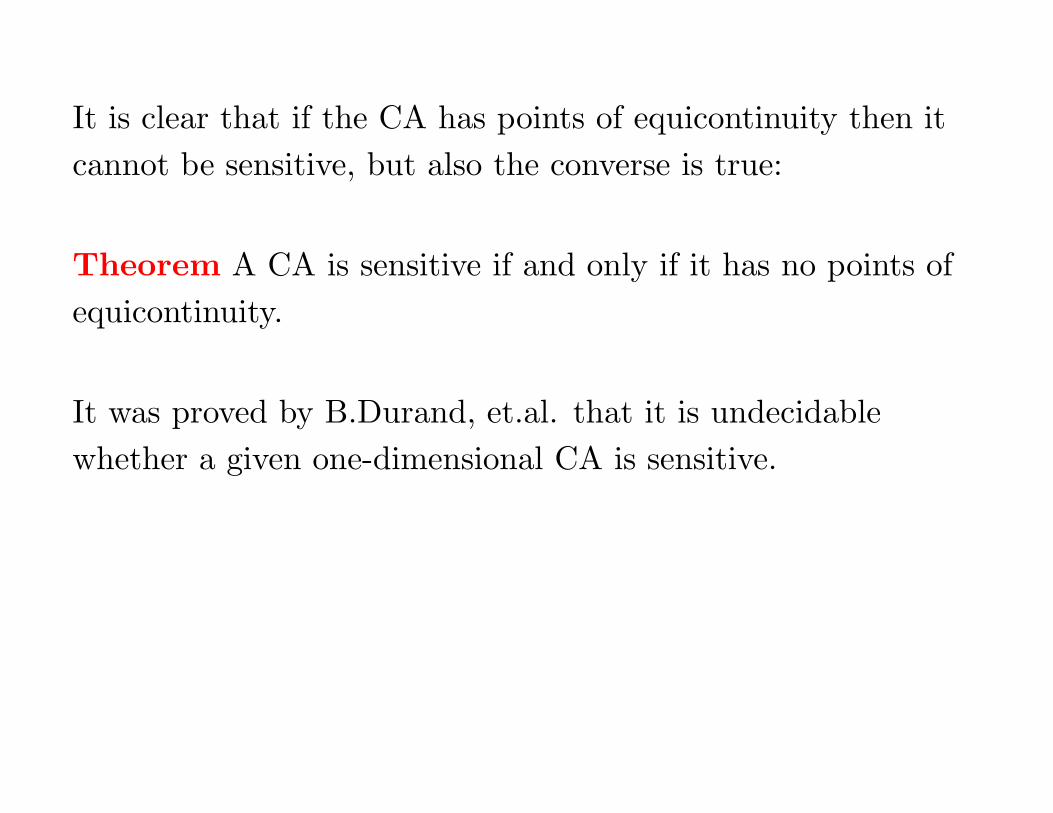
It is clear that if the CA has points of equicontinuity then it
cannot be sensitive, but also the converse is true:
Theorem A CA is sensitive if and only if it has no points of
equicontinuity.
It was proved by B.Durand, et.al. that it is undecidable
whether a given one-dimensional CA is sensitive.
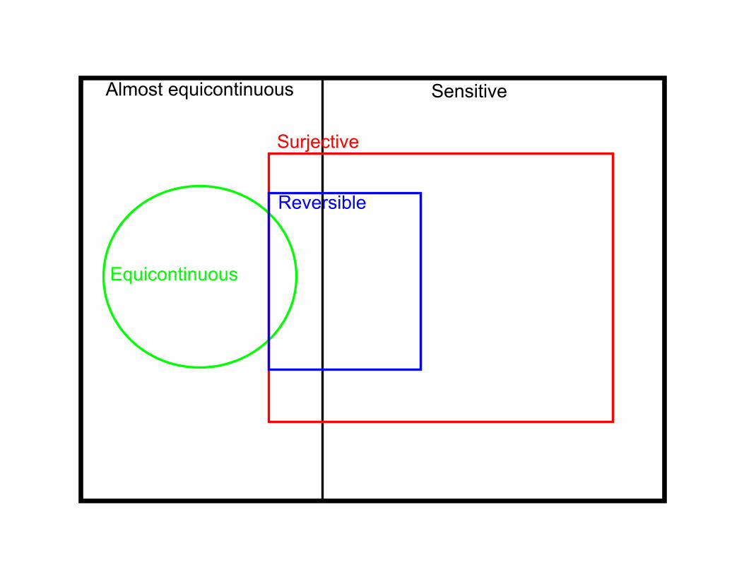
Almost equicontinuous
Equicontinuous
Surjective
Sensitive
Reversible
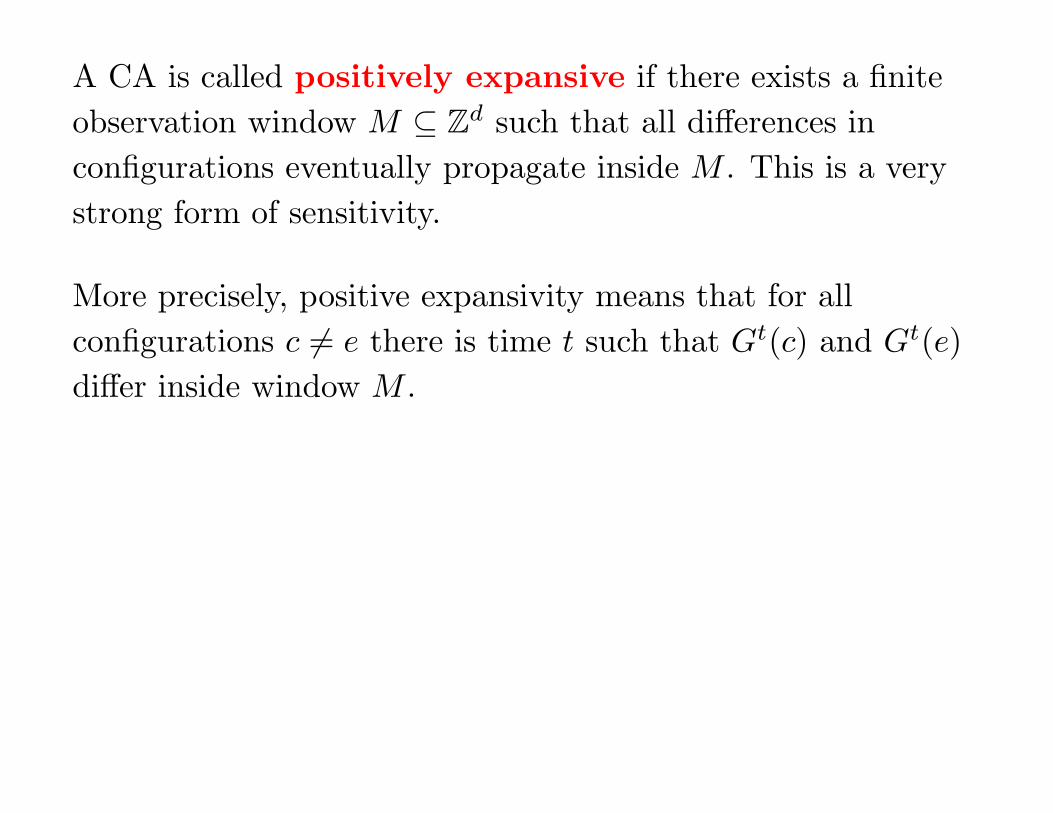
A CA is called positively expansive if there exists a finite
observation window M ⊆ Zd such that all differences in
configurations eventually propagate inside M . This is a very
strong form of sensitivity.
More precisely, positive expansivity means that for all
configurations c 6= e there is time t such that Gt(c) and Gt(e)
differ inside window M .
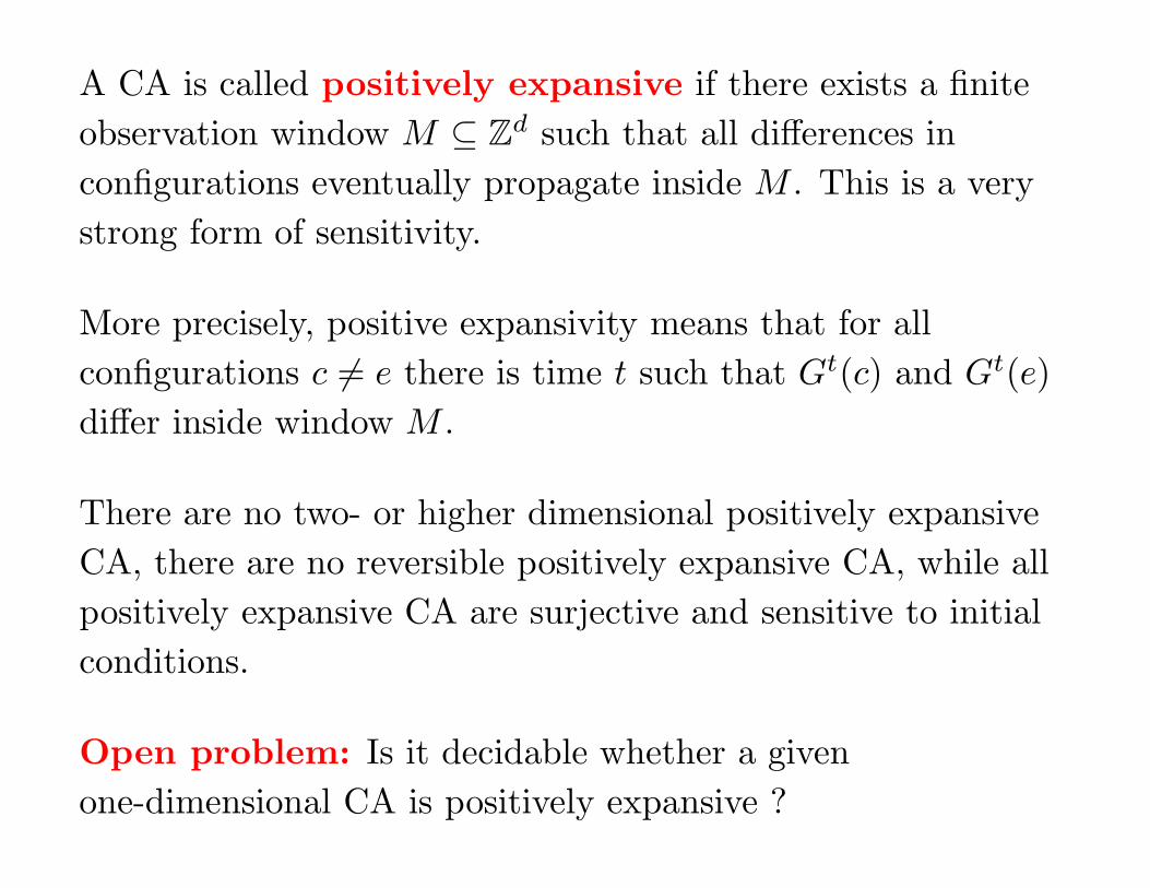
There are no two- or higher dimensional positively expansive
CA, there are no reversible positively expansive CA, while all
positively expansive CA are surjective and sensitive to initial
conditions.
Open problem: Is it decidable whether a given
one-dimensional CA is positively expansive ?
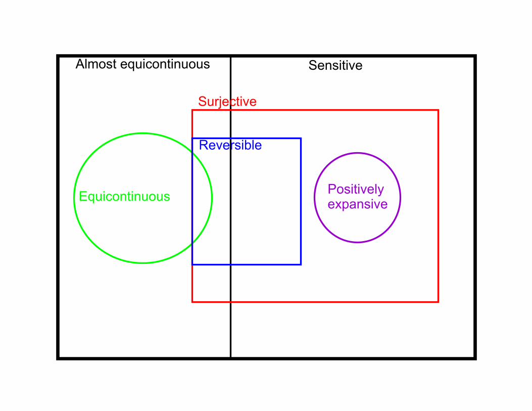
Almost equicontinuous
Equicontinuous
Surjective
Sensitive
Reversible
Positivelyexpansive
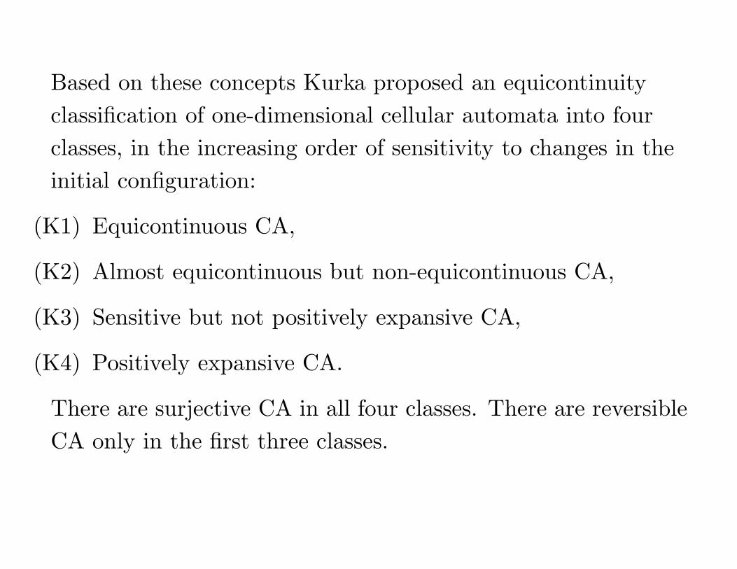
Based on these concepts Kurka proposed an equicontinuity
classification of one-dimensional cellular automata into four
classes, in the increasing order of sensitivity to changes in the
initial configuration:
(K1) Equicontinuous CA,
(K2) Almost equicontinuous but non-equicontinuous CA,
(K3) Sensitive but not positively expansive CA,
(K4) Positively expansive CA.
There are surjective CA in all four classes. There are reversible
CA only in the first three classes.
Finally, a property dealing with mixing of configurations can
be related to the equicontinuity classification: A CA is called
transitive if for any two cylinders U and V there exists time t
such that Gt(U) ∩ V 6= ∅.
Theorem (Blanchard, Maass) and Kurka: Every positive
expansive CA is transitive. Every transitive CA is surjective
and sensitive.
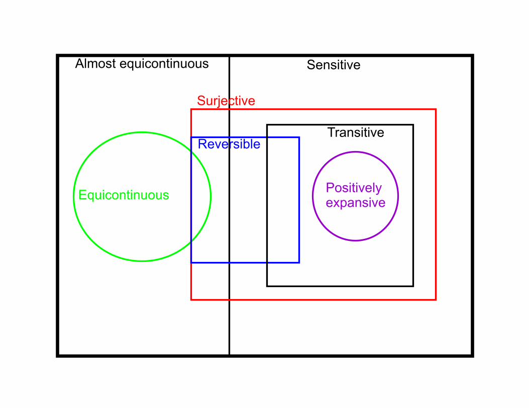
Almost equicontinuous
Equicontinuous
Surjective
Sensitive
Reversible
Positivelyexpansive
Transitive
Different definitions of chaotic systems exist. A widely used
definition by Devaney defines a dynamical system to be
chaotic if
(1) it is transitive,
(2) temporally periodic points are dense,
(3) it is sensitive to initial conditions.
Because in CA transitivity implies sensitivity so only
conditions (1) and (2) remain.
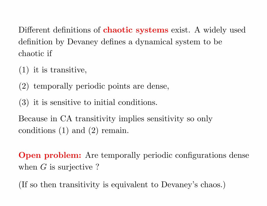
Open problem: Are temporally periodic configurations dense
when G is surjective ?
(If so then transitivity is equivalent to Devaney’s chaos.)
Limit sets. . . under construction. . .
Conclusion
There are many topics not covered in this tutorial, many
advanced results were not discussed, and many variants of the
basic definitions were not mentioned. Topics left out include,
for example,
• language recognition by cellular automata,
• linear cellular automata (=additive rules),
• intrinsic universality in cellular automata,
• error resilience in cellular automata
• asynchronous and stochastic CA,
• quantum CA,

• CA on Cayley graphs,
• dynamics under alternative topologies,
• firing squad synchronization problem and other cellular
algorithms,
• measure theoretic approach.
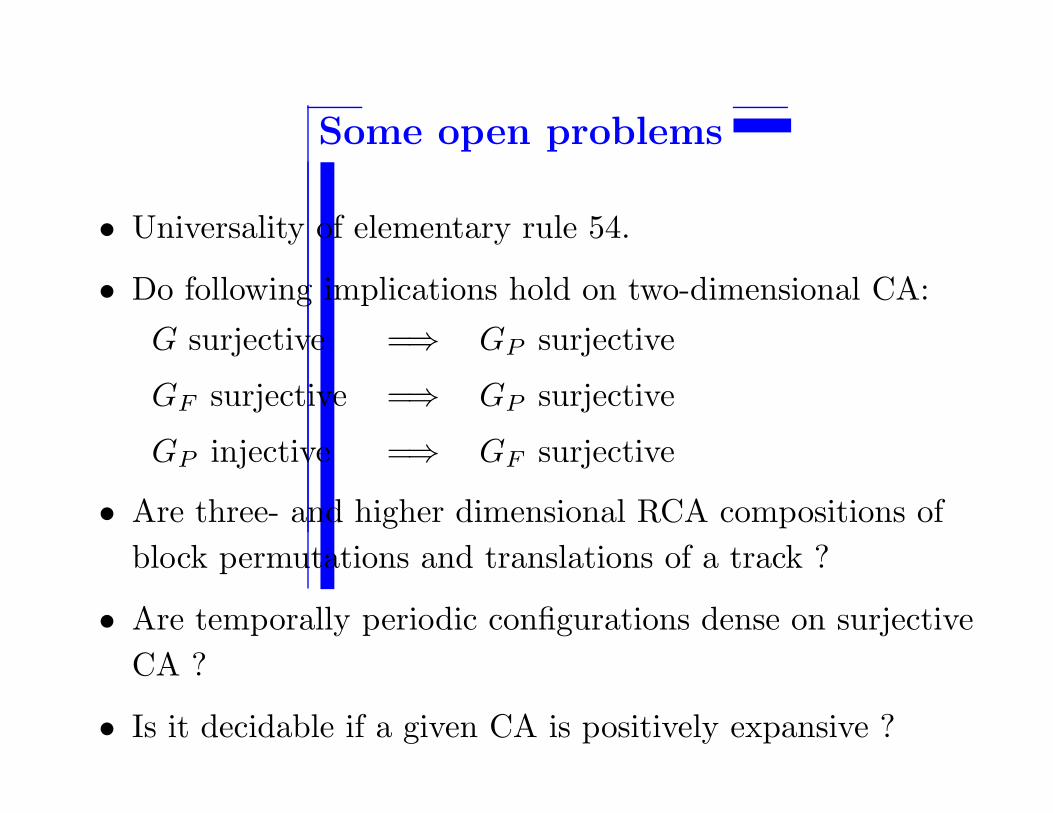
Some open problems
• Universality of elementary rule 54.
• Do following implications hold on two-dimensional CA:
G surjective =⇒ GP surjective
GF surjective =⇒ GP surjective
GP injective =⇒ GF surjective
• Are three- and higher dimensional RCA compositions of
block permutations and translations of a track ?
• Are temporally periodic configurations dense on surjective
CA ?
• Is it decidable if a given CA is positively expansive ?