Cellular AutomataCellular Automata

Cellular Automata?Cellular Automata?

• CA are computer simulations that try to emulate CA are computer simulations that try to emulate the way the laws of nature are supposed to the way the laws of nature are supposed to work in nature. work in nature.

• They can help us explore if the reductionist They can help us explore if the reductionist approach that scientific research has taken is approach that scientific research has taken is actually realistic.actually realistic.

Why CA?Why CA?

• Can we really imagine our fascinating, complex Can we really imagine our fascinating, complex and seemingly random world as created by a and seemingly random world as created by a small set of relatively simple rules?small set of relatively simple rules?

• rough way nature emulationrough way nature emulation• they can give us an idea of how reasonable the they can give us an idea of how reasonable the

thought of a world governed by simple rules isthought of a world governed by simple rules is

Short HistoryShort History

• CA were the invention of CA were the invention of John von Neumann John von Neumann around 1950 following a around 1950 following a suggestion of Stan Ulamsuggestion of Stan Ulam

• von Neumann was looking von Neumann was looking for a model of computation for a model of computation that could act on its own that could act on its own “matter”“matter”

World Before CAWorld Before CA

• Before von Neumann’s CA, the Before von Neumann’s CA, the standard model of computation standard model of computation was the Turing machinewas the Turing machine

• A Turing machine is a model of A Turing machine is a model of computation named after Alan computation named after Alan Turing, a British mathematician Turing, a British mathematician who helped break the German’s who helped break the German’s Secret “Enigma” codes in WWIISecret “Enigma” codes in WWII

Universal Turing MachinesUniversal Turing Machines

DataData(e.g., resignation letter)(e.g., resignation letter)

ProgramProgram(e.g., Microsoft Word)(e.g., Microsoft Word)

Are they really this different?Are they really this different?

No, No, they’re all just 0s and 1s!they’re all just 0s and 1s!

Is CA Better than TM?Is CA Better than TM?

• TM cannot alter themselvesTM cannot alter themselves• TM cannot build other computers although they can TM cannot build other computers although they can

simulate other TMssimulate other TMs• Although TMs are a standard model of computation, Although TMs are a standard model of computation,

they do not mirror the behavior of complex systems they do not mirror the behavior of complex systems – Turing Machines do not have feedback mechanisms to alter Turing Machines do not have feedback mechanisms to alter

their own behaviortheir own behavior

• A CA has the capability of altering itself – it does not A CA has the capability of altering itself – it does not have a distinction between structural parts and data,have a distinction between structural parts and data,

TM differs program and its dataTM differs program and its data

Stephen Wolfram Stephen Wolfram

• Key CA researcherKey CA researcher• Born in 1959 in LondonBorn in 1959 in London• First paper at age 15First paper at age 15• Ph.D. at 20Ph.D. at 20• Youngest recipient of MacArthur ‘young genius’ awardYoungest recipient of MacArthur ‘young genius’ award• Worked at Caltech and PrincetonWorked at Caltech and Princeton• Owner of Mathematica (Wolfram Research)Owner of Mathematica (Wolfram Research)• Fantastic publication record … until …Fantastic publication record … until …• 1988 when he stopped publishing in scientific journals1988 when he stopped publishing in scientific journals

CA decompositionCA decomposition

• DomainDomain– 1D: row, ring 1D: row, ring – 2D: rectangle, torus, …2D: rectangle, torus, …– 3D: volume3D: volume

• Cell = domain elementCell = domain element• NeighborhoodNeighborhood• Cell stateCell state• Initial state (condition)Initial state (condition)• Cell program (rule)Cell program (rule)• Discrete time evolutionDiscrete time evolution

Most Simple CAMost Simple CA

• 1D binary row domain1D binary row domain• Neighborhood = cell itselfNeighborhood = cell itself

Rule

LineThe first line is always given. This is what is called the ‘initial condition’.

This rule is trivial. It means black remains black and grey remains grey.

Time 0

Time 1

Time 2

This is how the Cellular Automaton evolves

1D Binary Cellular Automata1D Binary Cellular Automata

• 2 states2 states• Neighborhood of 1 cellNeighborhood of 1 cell

– 2222 possible programs possible programs– No space dependence No space dependence a bit boring a bit boring

• Neighborhood of 2 cellsNeighborhood of 2 cells– elementary space dependenceelementary space dependence– 2244 possible programs possible programs

• Neighborhood of 3 cellsNeighborhood of 3 cells– mostly usedmostly used– Sufficient space dependenceSufficient space dependence

Wolfram’s 1D Binary CAWolfram’s 1D Binary CA

• Program exampleProgram example

• Neighbourhood combnationsNeighbourhood combnations

• 2288 possible rules (programs) possible rules (programs)

The Wolfram NomenclatureThe Wolfram Nomenclature

• Rule = number Rule = number 0,2550,255• Example: rule 90Example: rule 90

= 2+8+16+64 = 90

Value 1

28

Value 6

4

Value 1

6

Value 3

2

Value 8

Value 4

Value 2

Value 1

Rule 254Rule 254

• Rule:Rule:

• Initial condition:Initial condition:

• Applying the rule 254:Applying the rule 254:

254:

Rule 254 EvolutionRule 254 Evolution254:

Time 0

Time 1

Time 2

Time 3

Rule 90Rule 90

• What does this form?What does this form?

• Initial conditionInitial condition

Rule 90:

Guess the Pattern!Guess the Pattern!

Rule 90 EvolutionRule 90 Evolution

9 Time Steps

Rule 90 Ad InfinitumRule 90 Ad Infinitum

• Sierpinski Gasket PatternSierpinski Gasket Pattern

Irregular Patterns?Irregular Patterns?

• Rule 30Rule 30

Rule 30:

Applying Rule 30Applying Rule 30

30:

Rule 30 EvolutionRule 30 Evolution

Rule 30 Ad InfinitumRule 30 Ad Infinitum

While one side has repetitive patterns, the other side appears random.

Zoom of the Regular RegionZoom of the Regular Region

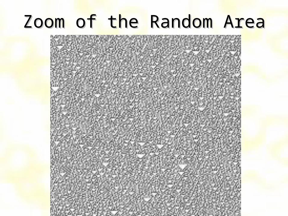
Zoom of the Random AreaZoom of the Random Area

Other RulesOther Rules

Rule Atlas (1)Rule Atlas (1)

Rule Atlas (2)Rule Atlas (2)

Rule Atlas (3)Rule Atlas (3)

• 256 rules256 rules• Same initial conditionSame initial condition

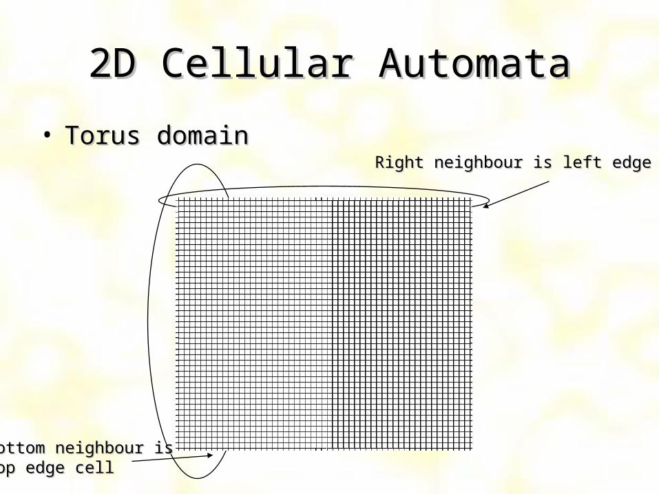
2D Cellular Automata2D Cellular Automata

• Torus domainTorus domainRight neighbour is left edge cellRight neighbour is left edge cell

Bottom neighbour isBottom neighbour istop edge celltop edge cell

2D Binary CA2D Binary CA

• Domain = torus bitmapDomain = torus bitmap• NeighbourhoodNeighbourhood

– cell and its 4 (Von Neumann) or 8 neighbors (Moore)cell and its 4 (Von Neumann) or 8 neighbors (Moore)– 4-neighborhood used mostly4-neighborhood used mostly

• Program = 2Program = 255 binary vector binary vector• 223232 possible programs (transition rules) possible programs (transition rules)

Well Known Instance:Well Known Instance:Conway’s Game of LifeConway’s Game of Life

John H. Conway

Life RulesLife Rules

• Each step: cell lives or diesEach step: cell lives or dies

• Alive Cell = 1, Dead cell = 0Alive Cell = 1, Dead cell = 0

• Three simple rulesThree simple rules– dies if # of alive neighbour cells =< 2dies if # of alive neighbour cells =< 2 (loneliness)(loneliness)– dies if # of alive neighbour cells >= 5 (overcrowding)dies if # of alive neighbour cells >= 5 (overcrowding)– lives is # of alive neighbour cells = 3 (procreation)lives is # of alive neighbour cells = 3 (procreation)

Rule ExamplesRule Examples

• loneliness (dies if #alive =< 2)

• overcrowding (dies if #alive >= 5)

• procreation (lives if #alive = 3)

Life PatternsLife Patterns

block pond ship eater

StableStable

time = 1 time = 2

PeriodicPeriodic

Time = 1 time = 2 time = 3 time = 4 time = 5

MovingMoving

Majority RuleMajority Rule

• 1 if 5 or more Moore neighbours and self are 1,1 if 5 or more Moore neighbours and self are 1,• 0 if 5 or more Moore neighbours and self are 0 0 if 5 or more Moore neighbours and self are 0 • Initial state: white noise (~50 % & zeroes)Initial state: white noise (~50 % & zeroes)

→→

Random Majority RuleRandom Majority Rule

• if 4 neighbours 0 and 4 1, new state random

→→

Multistate 2D CA PatternsMultistate 2D CA Patterns

The Segregation ModelThe Segregation Model

• Grid 500 by 500Grid 500 by 500• 1500 agents, 10501500 agents, 1050 greengreen, 450, 450 redred

– 1000 vacant patches1000 vacant patches

• Each agent has a Each agent has a tolerancetolerance– AA greengreen agent is ‘happy’ when the ratio of agent is ‘happy’ when the ratio of greensgreens to to

redsreds in its Moore neighbourhood is more than its in its Moore neighbourhood is more than its tolerancetolerance

– and vice versa forand vice versa for redsreds

AggregationAggregation

• Randomly allocateRandomly allocate redsreds andand greensgreens to patchesto patches• With a tolerance of 40%:With a tolerance of 40%:

– An agent is happy when more than 3/8 ( = 37.5%) of An agent is happy when more than 3/8 ( = 37.5%) of its neighbours are of the same colourits neighbours are of the same colour

• Then the average number of neighbours of the Then the average number of neighbours of the same colour issame colour is 58%58% (about 5)(about 5)

• And aboutAnd about 18%18% of the agents are unhappyof the agents are unhappy

TippingTipping

• Unhappy agents move along a random walk to Unhappy agents move along a random walk to a patch where they are happya patch where they are happy

• Emergence is a result of ‘tipping’Emergence is a result of ‘tipping’– If one If one redred enters a neighbourhood with 2 enters a neighbourhood with 2 redsreds

already there, a previously happy already there, a previously happy greengreen will become will become unhappy and move elsewhere, either contributing to unhappy and move elsewhere, either contributing to a a greengreen cluster or possibly upsetting previously cluster or possibly upsetting previously happy happy redsreds and so on… and so on…

EmergenceEmergence

• Values of tolerance above 30% Values of tolerance above 30% give clear display of clustering: give clear display of clustering: ‘ghettos’‘ghettos’

• Even though agents tolerate 30% Even though agents tolerate 30% of their neighbours being of the of their neighbours being of the other colour in their other colour in their neighbourhood, the average neighbourhood, the average percentage of same-colour percentage of same-colour neighbours is typically 75 - 80% neighbours is typically 75 - 80% after everyone has moved to a after everyone has moved to a satisfactory location (risen from satisfactory location (risen from 58% before relocations)58% before relocations)

Dynamic Social ImpactDynamic Social Impact

for individual for individual aa, impact of ‘supporters’, , impact of ‘supporters’, iiasas

isisias

Sj

daj2

j1

jN

2

and the same for the impact of and the same for the impact of ‘opposers’,‘opposers’, iiaoao

agent agent a a changes state if changes state if iiaoao >> iiasas

Social Impact PatternsSocial Impact Patterns

Random starting attitudes,with 30% white

Final (stable) attitudes,with 16% white

More from the Game TheoryMore from the Game Theory

The Prisoner’sThe Prisoner’s

DilemmaDilemma3

3

5

0

0

5

1

1A c

o-op

erat

es(d

oesn

’t c

onfe

ss)

A d

efec

ts(c

onfe

sses

)

B co-operates(doesn’t confess)

B defects(confesses)

Length of time in prison

Playing the Game OncePlaying the Game Once

• The rational action is to confess, The rational action is to confess, regardless of the other’s choice regardless of the other’s choice (obtaining a sentence of 3 years rather (obtaining a sentence of 3 years rather than 5, or no prison rather than 1 year).than 5, or no prison rather than 1 year).

• Therefore both choose to confess, Therefore both choose to confess, going to prison for 3 years, although if going to prison for 3 years, although if both refused to confess, they would both refused to confess, they would both be sentenced to only 1 year in both be sentenced to only 1 year in prison.prison.

3

3

5

00

5

1

1

A c

o-op

erat

es(d

oesn

’t c

onfe

ss)

A d

efec

ts(c

onfe

sses

)

B co-operates(doesn’t confess)

B defects(confesses)

Iterated Prisoner’s DilemmaIterated Prisoner’s Dilemma

• If the same people repeatedly play the IPD If the same people repeatedly play the IPD game, they can learn the other’s strategy.game, they can learn the other’s strategy.

• What’s the best strategy? Tit-for-TatWhat’s the best strategy? Tit-for-Tat• 1st move: cooperate1st move: cooperate• subsequent move: copy opponent’s previous movesubsequent move: copy opponent’s previous move

– Tit-for-tat is best against other strategies, Tit-for-tat is best against other strategies, provided provided that there is no noisethat there is no noise (perfect communication) (perfect communication)

• Note that this assumes that agents can Note that this assumes that agents can recognise each otherrecognise each other– Not a trivial requirementNot a trivial requirement

Evolving strategiesEvolving strategies

• 1000100022 agents arranged in a grid. At every step, each agents arranged in a grid. At every step, each agent plays an IPD with a large random sample of other agent plays an IPD with a large random sample of other agents.agents.

• Each agent remembers the last three moves of its IPD Each agent remembers the last three moves of its IPD opponent and follows one of the 2opponent and follows one of the 215 15 possible different possible different strategiesstrategies

• At the end of each step, an agent randomly finds At the end of each step, an agent randomly finds another and switches to the other agent’s strategy if that another and switches to the other agent’s strategy if that is better (higher total payoff)is better (higher total payoff)

• Calculation of difference between payoff is subject to Calculation of difference between payoff is subject to noisenoise

• New strategies mutate (noisy transmission)New strategies mutate (noisy transmission)

Lattice Gas Cellular AutomataLattice Gas Cellular Automata

• Dynamics of boolean quantities on a regular lattice.

• The evolution is synchronous and based on discrete time steps.

Max. 4 particles at each lattice site,

Unitary speed in the particle’s direction

Example : HPP (Hardy, Pomeau, de Pazzis; 1986)(Historical model: suffers from inconsistensies at a macroscopical level)

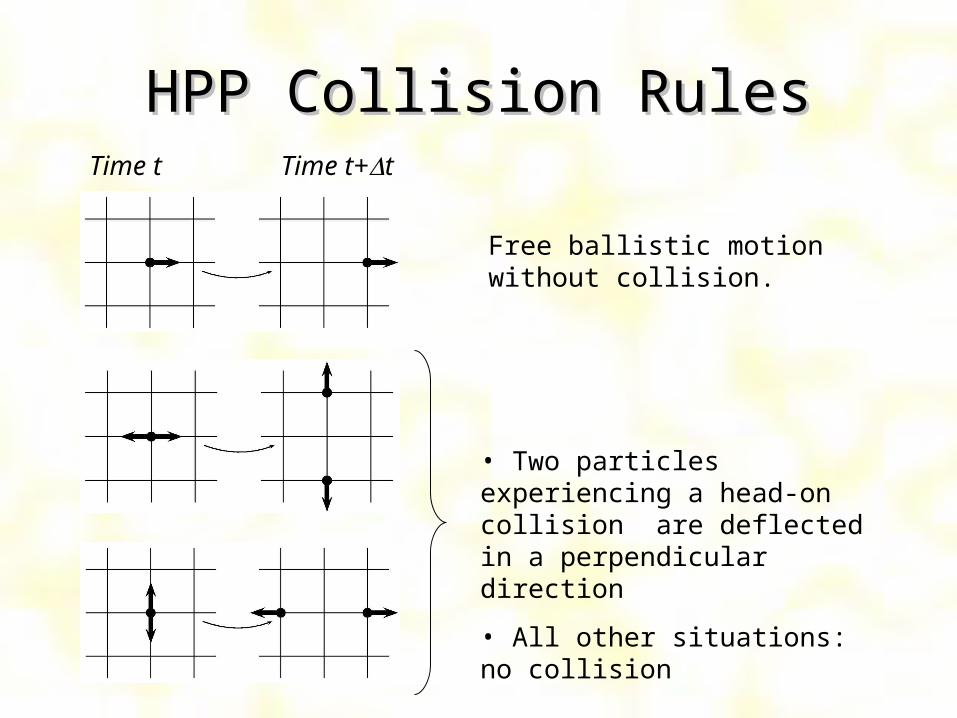
HPP Collision RulesHPP Collision Rules

Free ballistic motion without collision.

Time t Time t+t

• Two particles experiencing a head-on collision are deflected in a perpendicular direction

• All other situations: no collision

Evaluation of a LGCAEvaluation of a LGCA

• Realistic macroscopical fluid dynamics are obtained when the lattice is fine enough.

• Problem : averaging over big lattice domains needed.

Discrete particle distribution Averaged “macroscopical” values

From LGCA to LBMFrom LGCA to LBMIdeaIdea : implement the dynamics directly on the average values.

AdvantagesAdvantages :

• One lattice node represents particle densities: discrete dynamics are replaced by a smooth flow.

• Less averaging needed, increased performance.

Disadvantages :Disadvantages :

• Higher order correlations between particles are neglected.

• Numerical instabilities appear.

LGCA: Boolean quantities ni

LBM: Real-valued quantities fi

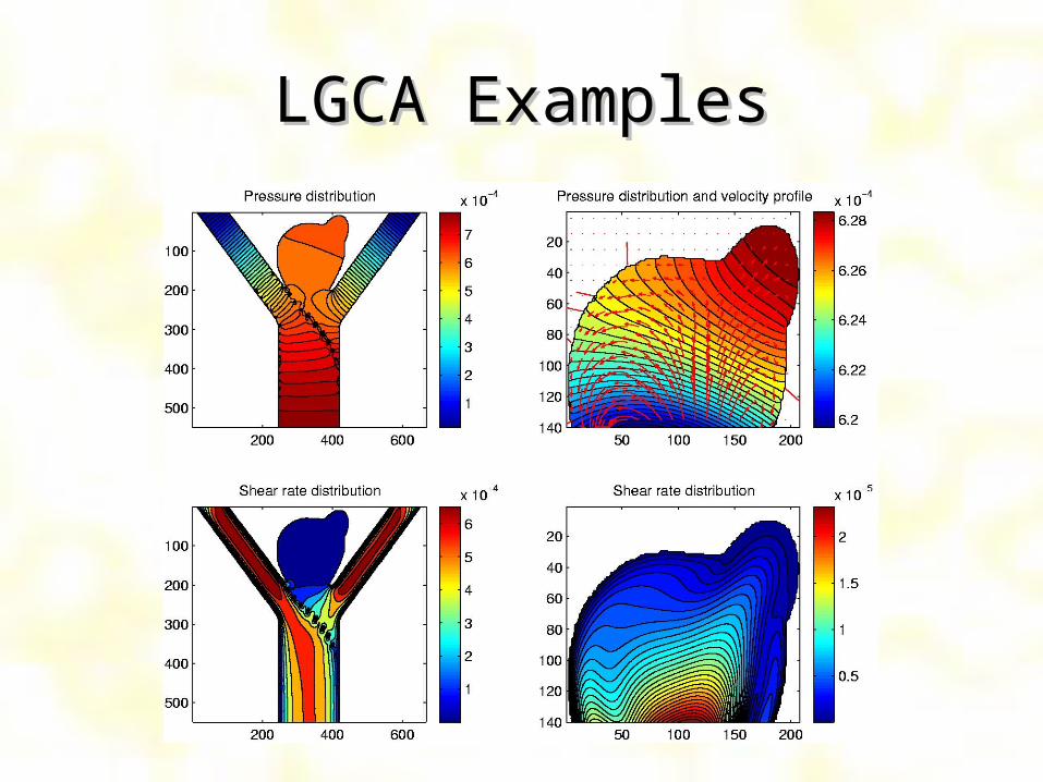
LGCA ExamplesLGCA Examples

CA Binary TexturesCA Binary Textures

• Texture = visualization of the CA stateTexture = visualization of the CA state• NetLogo, StarLogo systems = IDE for CANetLogo, StarLogo systems = IDE for CA• General Language for CA?General Language for CA?• Raw language = Wolfram’s nomenclatureRaw language = Wolfram’s nomenclature• Most simpleMost simple

– torus domaintorus domain– binary statebinary state– 4-neighborhood4-neighborhood

Binary CA ProgramsBinary CA Programs

• www.cg.tuwien.ac.at/studentwork/CESCG/CESCG-2000/PBorovsky

• Cell + 4 neigbours = 5-bit neighborhoodCell + 4 neigbours = 5-bit neighborhood

• Program = 2Program = 255 bits bits• How many such binary CA program there are?How many such binary CA program there are?• 223232 (4 294 967 296) possible programs (4 294 967 296) possible programs

Random Program GenerationRandom Program Generation

• Program = 32-bit Program = 32-bit numbernumber

• Random generationRandom generation• Initial state = ?Initial state = ?

– white noise white noise (statistical balance)(statistical balance)

• Patterns = ?Patterns = ?– Complex imagesComplex images– e.g. reaction-diffusione.g. reaction-diffusion

Nice Pattern RecognitionNice Pattern Recognition

• Nearly 20 % of random programs Nearly 20 % of random programs

interesting patterninteresting pattern• Characteristics of these programs = ?Characteristics of these programs = ?• One possibility = study of convergenceOne possibility = study of convergence• System = repeating, if it repeats a sequence of System = repeating, if it repeats a sequence of

states (after finite evolution)states (after finite evolution)• Convergent system = 1 state repetitionConvergent system = 1 state repetition

Convergence DeterminitionConvergence Determinition

• Reverse pattern completing algorithmReverse pattern completing algorithm• Input = program, output = converges / notInput = program, output = converges / not• Filling the space with the stable rulesFilling the space with the stable rules• Stable rule do not change the neighbourhoodStable rule do not change the neighbourhood

• Filling the space by 0 and 1 (substitution of “?”)Filling the space by 0 and 1 (substitution of “?”)• Initial condition = the final stable patternInitial condition = the final stable pattern

Randomness on any CA?Randomness on any CA?

• Binary automata = 32-bit programsBinary automata = 32-bit programs– CA Interpreter: 32 cases in the neighborhoodCA Interpreter: 32 cases in the neighborhood

• More states for color texturesMore states for color textures• 256 states 256 states 2 24040-bit programs-bit programs

– CA Interpreter: too much cases in the neighborhoodCA Interpreter: too much cases in the neighborhood– Impossible to interpret the programs in the Wolframs Impossible to interpret the programs in the Wolframs

formatformat

• Other language for CA?Other language for CA?– Simple syntaxSimple syntax– Easy to codeEasy to code– Easy to generate random programsEasy to generate random programs

CA Language ProposalCA Language Proposal

• Cell:Cell:– State = floating-point variable (color)State = floating-point variable (color)– Multiple states (at least 6 states for reaction-diffusion)Multiple states (at least 6 states for reaction-diffusion)– Ability to read variables from 8 neighborsAbility to read variables from 8 neighbors

• ProgramProgram– Set of rules for each variableSet of rules for each variable– Evolution from time 0Evolution from time 0– Variable ‘random’ (e.g. initial state)Variable ‘random’ (e.g. initial state)

• CA extensionCA extension– Cell knows its position (x,y), time, …Cell knows its position (x,y), time, …

Texture Language ProposalTexture Language Proposal

TLA Program ExampleTLA Program Example

• Averaged Noise in TLAAveraged Noise in TLA

• Uses 1 variableUses 1 variable• Rule = conditionalRule = conditional• Access of other cells: left[i], right[i],…Access of other cells: left[i], right[i],…• Access of own cell: center[i]Access of own cell: center[i]

TLA InterpreterTLA Interpreter

• Slightly different conditional than in C/C++Slightly different conditional than in C/C++– Never returns from nested branchNever returns from nested branch

• VisualizationVisualization– LayersLayers– Layer Layer ii = variable = variable i i – Greyscale adaptive paletteGreyscale adaptive palette

TLA UsageTLA Usage

• NoisesNoises• Reaction-diffusionReaction-diffusion• Implicit phenomenaImplicit phenomena• UnsuitableUnsuitable

– Explicit objectsExplicit objects– e.g. midpoint diamond e.g. midpoint diamond