cell acquisition and synchronization for …1134090/fulltext01.pdfcell acquisition and...
TRANSCRIPT
Master of Science Thesis in Communication SystemsDepartment of Electrical Engineering, Linköping University, 2017
Cell Acquisition andSynchronization forUnlicensed NB-IoT
Eskil Jörgensen
Master of Science Thesis in Communication Systems
Cell Acquisition and Synchronization for Unlicensed NB-IoT
Eskil Jörgensen
LiTH-ISY-EX--17/5082--SE
Supervisor: Daniel Verenzuelaisy, Linköpings universitet
Y.-P. Eric WangEricsson, Inc
Examiner: Erik G. Larssonisy, Linköpings universitet
Division of Communication SystemsDepartment of Electrical Engineering
Linköping UniversitySE-581 83 Linköping, Sweden
Copyright © 2017 Eskil Jörgensen

Abstract
Narrowband Internet-of-Things (NB-IoT) is a new wireless technology designedto support cellular networks with wide coverage for a massive number of verycheap low power user devices. Studies have been initiated for deployment of NB-IoT in unlicensed frequency bands, some of which demand the use of a frequency-hopping scheme with a short channel dwell time. In order for a device to connectto a cell, it must synchronize well within the dwell time in order to decode thefrequency-hopping pattern. Due to the significant path loss, the narrow band-width and the device characteristics, decreasing the synchronization time is achallenge. This thesis studies different methods to decrease the synchronizationtime for NB-IoT without increasing the demands on the user device. The studyshows how artificial fast fading can be combined with denser reference signallingin order to achieve improvements to the cell acquisition and synchronization pro-cedure sufficient for enabling unlicensed operation of NB-IoT.
iii


Sammanfattning
Narrowband Internet-of-Things (NB-IoT) är en ny trådlös teknik som är desig-nad för att hantera mobilnät med vidsträckt täckning för ett massivt antal myc-ket billiga och strömsnåla användarenheter. Studier har inletts för att opereraNB-IoT i olicensierade frekvensband, varav några kräver att frekvenshoppandespridningsspektrum, med kort uppehållstid per kanal, används. För att en använ-darenhet ska kunna ansluta till en basstation måste den slutföra synkronisings-fasen inom uppehållstiden, så att basstationens hoppmönster kan avkodas. Pågrund utav den stora signalförsvagningen, den smala bandbredden och använda-renhetens egenskaper är det en stor utmaning att förkorta synkroniseringstiden.Detta examensarbete studerar olika metoder för att förkorta synkroniseringsti-den i NB-IoT utan att öka kraven på användarenheten. Arbetet visar att artificiellsnabb-fädning kan kombineras med tätare referenssignalering för att uppnå för-bättringar i synkroniseringsprocessen som är tillräckliga för att möjliggöra ope-ration av NB-IoT i olicensierade frekvensband.
v


Acknowledgments
I would like to express my thanks to the whole team at Ericsson Research SiliconValley for a great time in their friendly and exciting working environment. Inparticular, I would like to thank the radio team for many interesting discussionsand the large amount of constructive feedback they offered. My greatest thanksgoes to my supervisor Eric Wang for his continuous support and genuine interestin the study. He unhesitatingly and accurately answered any questions I came upwith, and those were many.
I also would like to thank my academic supervisor Daniel Verenzuela and my ex-aminer Erik G. Larsson, for providing valuable feedback on the thesis while beingflexible and patient with my own way of working. Finally, I want to thank Gun-nar Bark, Ali Khayrallah and Thomas Cheng for actively supporting the initiativeto make this project possible in the first place.
Santa Clara, June 2017Eskil Jörgensen
vii


Contents
Notation xiii
1 Introduction 11.1 Motivation . . . . . . . . . . . . . . . . . . . . . . . . . . . . . . . . 11.2 Purpose . . . . . . . . . . . . . . . . . . . . . . . . . . . . . . . . . . 21.3 Problem Formulation . . . . . . . . . . . . . . . . . . . . . . . . . . 21.4 Limitations . . . . . . . . . . . . . . . . . . . . . . . . . . . . . . . . 31.5 Thesis Outline . . . . . . . . . . . . . . . . . . . . . . . . . . . . . . 4
2 Synchronization in OFDM Systems 52.1 Synchronization in General Terms . . . . . . . . . . . . . . . . . . . 5
2.1.1 Synchronized Communication . . . . . . . . . . . . . . . . . 62.2 Orthogonal Frequency-Division Multiplexing . . . . . . . . . . . . 8
2.2.1 OFDM Synchronization Tasks . . . . . . . . . . . . . . . . . 92.2.2 Effects of Deficient Synchronization . . . . . . . . . . . . . 12
2.3 Cellular OFDM and Initial Cell Search . . . . . . . . . . . . . . . . 132.4 OFDM Downlink Methods . . . . . . . . . . . . . . . . . . . . . . . 14
2.4.1 Pilot Characteristics . . . . . . . . . . . . . . . . . . . . . . . 17
3 Narrowband Internet of Things 193.1 LTE, 5G and mMTC . . . . . . . . . . . . . . . . . . . . . . . . . . . 193.2 Downlink Physical Layer . . . . . . . . . . . . . . . . . . . . . . . . 21
3.2.1 Physical Channels and Signals . . . . . . . . . . . . . . . . . 223.3 Synchronization in NB-IoT . . . . . . . . . . . . . . . . . . . . . . . 23
3.3.1 Base Sequence . . . . . . . . . . . . . . . . . . . . . . . . . . 243.3.2 Code Cover . . . . . . . . . . . . . . . . . . . . . . . . . . . 243.3.3 Reciever NPSS Processing . . . . . . . . . . . . . . . . . . . 243.3.4 Receiver NSSS Processing . . . . . . . . . . . . . . . . . . . 273.3.5 Master Information Block . . . . . . . . . . . . . . . . . . . 27
4 Operation in Unlicensed Spectrum 294.1 Frequency Bands . . . . . . . . . . . . . . . . . . . . . . . . . . . . . 294.2 Regulations . . . . . . . . . . . . . . . . . . . . . . . . . . . . . . . . 30
ix

x Contents
4.2.1 US ISM Bands . . . . . . . . . . . . . . . . . . . . . . . . . . 314.2.2 EU Short Range Devices . . . . . . . . . . . . . . . . . . . . 33
4.3 Conclusions . . . . . . . . . . . . . . . . . . . . . . . . . . . . . . . 33
5 Temporal Diversity 355.1 Coherent Combining . . . . . . . . . . . . . . . . . . . . . . . . . . 355.2 Method 1: NPSS Densification . . . . . . . . . . . . . . . . . . . . . 365.3 Method 2: NPSS Enhancement . . . . . . . . . . . . . . . . . . . . . 37
5.3.1 Design Guidelines . . . . . . . . . . . . . . . . . . . . . . . . 375.3.2 Minimum-sidelobe Binary Codes . . . . . . . . . . . . . . . 385.3.3 Barker Codes . . . . . . . . . . . . . . . . . . . . . . . . . . 395.3.4 Proposal . . . . . . . . . . . . . . . . . . . . . . . . . . . . . 39
6 Spatial Diversity 416.1 Fading Channels in NB-IoT . . . . . . . . . . . . . . . . . . . . . . . 416.2 Motivation . . . . . . . . . . . . . . . . . . . . . . . . . . . . . . . . 436.3 Codebook Design . . . . . . . . . . . . . . . . . . . . . . . . . . . . 44
6.3.1 Grassmannian Line Packing . . . . . . . . . . . . . . . . . . 466.3.2 Hadamard Patterns . . . . . . . . . . . . . . . . . . . . . . . 46
6.4 Method 3: Artificial Fast Fading . . . . . . . . . . . . . . . . . . . . 46
7 Experimental Setup 497.1 Experiment Overview . . . . . . . . . . . . . . . . . . . . . . . . . . 49
7.1.1 Objectives and Methods . . . . . . . . . . . . . . . . . . . . 497.1.2 Experiment Procedure . . . . . . . . . . . . . . . . . . . . . 50
7.2 Simulation Setup . . . . . . . . . . . . . . . . . . . . . . . . . . . . 517.2.1 Basic Assumptions . . . . . . . . . . . . . . . . . . . . . . . 517.2.2 Varying Parameters . . . . . . . . . . . . . . . . . . . . . . . 53
8 Results 578.1 Prestudy . . . . . . . . . . . . . . . . . . . . . . . . . . . . . . . . . 57
8.1.1 Pulse Shaping . . . . . . . . . . . . . . . . . . . . . . . . . . 578.1.2 Target Latency . . . . . . . . . . . . . . . . . . . . . . . . . . 58
8.2 Method Comparison and Selection . . . . . . . . . . . . . . . . . . 598.2.1 NPSS Densification . . . . . . . . . . . . . . . . . . . . . . . 608.2.2 NPSS Enhancement . . . . . . . . . . . . . . . . . . . . . . . 608.2.3 Artificial Fast Fading . . . . . . . . . . . . . . . . . . . . . . 608.2.4 Candidate Selection . . . . . . . . . . . . . . . . . . . . . . . 61
8.3 Algorithm Fine-tuning . . . . . . . . . . . . . . . . . . . . . . . . . 618.3.1 Candidate 1 . . . . . . . . . . . . . . . . . . . . . . . . . . . 618.3.2 Candidate 2 . . . . . . . . . . . . . . . . . . . . . . . . . . . 62
8.4 Evaluation . . . . . . . . . . . . . . . . . . . . . . . . . . . . . . . . 63
9 Discussion and Conclusion 659.1 Results . . . . . . . . . . . . . . . . . . . . . . . . . . . . . . . . . . 65
9.1.1 Prestudy . . . . . . . . . . . . . . . . . . . . . . . . . . . . . 659.1.2 Method Selection . . . . . . . . . . . . . . . . . . . . . . . . 66

Contents xi
9.1.3 Algorithm Fine-Tuning . . . . . . . . . . . . . . . . . . . . . 669.1.4 Evaluation . . . . . . . . . . . . . . . . . . . . . . . . . . . . 66
9.2 The Work in a Wider Perspective . . . . . . . . . . . . . . . . . . . 679.3 Conclusions . . . . . . . . . . . . . . . . . . . . . . . . . . . . . . . 67
9.3.1 Answers to the Research Questions . . . . . . . . . . . . . . 679.3.2 Implications . . . . . . . . . . . . . . . . . . . . . . . . . . . 68
9.4 Future Work . . . . . . . . . . . . . . . . . . . . . . . . . . . . . . . 68
List of Figures 71
List of Tables 72
Bibliography 73


Notation
Sets, distributions and operators
Notation Definition
R The set of real numbersC The set of complex numbersT The circle group, T = {z ∈ C : |z| = 1}Sn The unit n-sphere, {x ∈ Rn+1 : ‖x‖ = 1}
Gr(r, V ) The set of r-dimensional subspaces of VCN (0, Γ ) Circularly-symmetric normal distributionE {X} Expectation of X
Var {X} Variance of XCov {X, Y } Covariance of X and Y
XH Hermitian transpose of matrix X‖x‖p p-norm of vector x|x| Absolute value of scalar xx′ Time derivative of x
Design parameters
Notation Definition
B Base sequences Code coverfc Carrier frequencyfs Sampling rateα Forgetting factorρ(τ) Synchronization metricwk Metric summation weightλG Genie detection thresholdλP Peak detection thresholdW Codebook matrix
xiii

xiv Notation
Abbrevations
Abbrevation Definition
3gpp 3rd Generation Partnership Project5g 5th Generation Mobile Networksbs Base Station
cazac Constant Amplitude Zero Autocorrelation Waveformcfo Carrier Frequency Offsetcp Cyclic Prefixcro Carrier Raster Offsetdl Downlinkecc Electronic Communications Committeeecdf Empirical Cumulative Distribution Functionegb Equal Gain Beamformingeirp Equivalent Isotropically Radiated Powererp Equivalent Radiated Powerfar False Alarm Ratefcc Federal Communications Commissionfhss Frequency-hopping Spread Spectrumgsm Global System for Mobile Communicationsici Intercarrier Interferenceics Initial Cell Searchisi Intersymbol Interferenceism Industrial, Scientific and Medicalitu International Telecommunication Unionlte Long-Term Evolutionmai Multiple-Access Interferencemcl Maximum Coupling Lossmf Merit Factormib Master Information Block
mmtc Massive Machine Type Communicationmtc Machine Type Communicationnb-iot Narrowband Internet of Thingsnb-iot-u NB-IoT in Unlicensed Spectrumnpss Narrowband Primary Synchronization Signalnsss Narrowband Secondary Synchronization Signalofdm Orthogonal Frequency-Division Multiplexingprb Physical Resource Blockpsl Peak Sidelobe Levelpst Primary Synchronization Timeqam Quadrature Amplitude Modulationrrc Root-raised-cosinesnr Signal-to-Noise Ratiosrd Short Range Devicesue User Equipmentul Uplink
1Introduction
This chapter will set the stage for the thesis by introducing the studied problem.The problem is first motivated by describing how the solution would help in theongoing developments within the field of wireless networks. The purpose of thestudy is then declared, followed by a particularized problem formulation. Thechapter ends with a precaution on the limitations of the study and an outline ofthe following chapters.
1.1 Motivation
During the last decade, there has been a rapid growth in the number of mobileconnected devices. This growth has been projected to last for years ahead, whichimplies great challenges for development in wireless communication technology.In the "IMT Vision for 2020" [1], one of three major upcoming use case categoriesis envisioned to be the so called massive machine type communication (mmtc).mmtc refers to connectivity for a large number of devices with high demands onaffordability, battery life and coverage — but with lower demands on throughputand latency.
Narrowband Internet of Things (nb-iot) is a new technology that was introducedby the 3rd Generation Partnership Project (3gpp) standards organization in itsRelease 13 as a candidate for enabling mmtc. A critical design feature for nb-iot is a synchronization scheme (consisting of signaling and algorithms) that issimple enough to meet the demands on device cost and power consumption, butrobust enough to perform under extreme coverage conditions.
In a typical cellular communications system such as nb-iot, cell acquisition andsynchronization is the first task a user needs to perform in order to connect to a
1

2 1 Introduction
cell. This task consists of a few subtasks: detection of a suitable cell to connectto; coarse and fine estimation of timing, frequency and phase for this cell; andacquirement of its specific cell ID. In order to facilitate these tasks, many cellu-lar systems employ carefully designed synchronization reference signals broad-casted by the base station of each cell. A series of studies were carried out withinthe 3gpp community to find such reference signals for nb-iot, that enable robustsynchronization by devices with low-end receivers. One of the main studies thatled to actual standardization of synchronization reference signals is [2].
Deployment of nb-iot in unlicensed bands (called nb-iot-u in this thesis) mightbe desirable as a way to provide more spectrum at a low cost and is now beinginvestigated in several organizations. Some of the bands that are under consid-eration have regulations that enforce wireless devices to use frequency hopping,limiting the dwell time on a single carrier frequency down to fractions of a sec-ond. For a nb-iot user to connect to the network, it must be able to synchronizeand detect the cell ID before it hops to a new carrier. The current synchronizationscheme, although being robust and computationally efficient, have been shownto exceed this time frame for some demanded coverage conditions [3]. The syn-chronization time thus need to be improved for nb-iot-u to be successful.
In order to increase the coverage of nb-iot and to facilitate adaption for unli-censed bands, studies of enhancing the current nb-iot synchronization designare of great interest.
1.2 Purpose
The purpose of this thesis is to aid the design of nb-iot-u by studying the per-formance of various methods for initial cell acquisition and synchronization innb-iot. The methods under consideration mainly refers to different synchroniza-tion signals on the transmitter side and different signal processing techniques onthe receiver side.
1.3 Problem Formulation
The main problem seen in today’s standard is considered to be synchronizationtime. Decreasing this time would require the receiver to have access to more infor-mative signals, to process current signals more effectively or to decrease demandson accuracy. Decreasing the accuracy will affect subsequent perceived signal-to-noise ratio (snr) — increasing communication error rates — and is not consid-ered an alternative in this study. More informative signals could be achieved byimproving the channel, increasing signal power or by changing the reference sig-nals at the transmitter. The latter would require an undesirable change to thecurrent nb-iot standard but is still a viable option. More effective processing ofcurrent signals on the other hand might require more expensive receiver devicesor a greater receiver power consumption, both of which are undesirable for mmtcusage. To address these problems, the following research questions are stated:
1.4 Limitations 3
• How can nb-iot synchronization time be decreased while keeping accuracyhigh and receiver complexity low?
• What methods could be good candidates for nb-iot-u?
• Would those candidates require a change of the current standard?
In order to answer these questions, we need well defined metrics. We define pri-mary synchronization time (pst) as the amount of time it takes for a user device,after the start of a cell search, to successfully acquire timing and frequency in-formation. What counts as successful is up to the receiver algorithm to decide,but this decision will affect the accuracy. To help us answer the first researchquestion, the 90th percentile of pst among devices is set as the main metric, butempirical cumulative distribution function (ecdf) plots or tables of the pst willbe provided. The 90th percentile is a common capability metric used for designof wireless systems to balance high robustness against low overhead. It is alsoa more reliable statistic under limited sample sizes, as compared to higher per-centiles.
The accuracy mentioned in the same question is measured by residual timingand frequency errors after successful synchronization. Our metric for accuracywill be false alarm rate1 (far), which we define as the fraction of devices havingresidual errors above a certain acceptable limit. The exact limit is set to make surethat communication can proceed under decent error rates and will be determinedin Chapter 7. A target far of 5% will serve as a guideline, this also being acommon trade-off between robustness and overhead.
The demand on receiver complexity will be met by choosing a baseline receiveralgorithm that is known to be cheap and then modify the algorithm in ways thatare guaranteed not to increase complexity significantly.
While the first question aims to study a variety of methods and compare themin a qualitative way, the second question aims to select from these methods twoor three specific configurations. These configurations will be evaluated quantita-tively using the specific requirements and conditions defined later in Section 4.3and Section 8.1, with the aim of having 90% of all users meeting these require-ments. The last question is easy to answer for a given method: new standardiza-tion is required only if the synchronization signals are changed.
1.4 Limitations
The thesis studies how the capability of current nb-iot synchronization can beextended. Since the capability of a system is determined by its limits, we willrestrict our study to the most challenging cases:
• Only low speed users, to increase the effect of prolonged deep fades.
• Only low snr, corresponding to a very large path loss.
1False alarms are often referred to as type I errors.

4 1 Introduction
However, due to time constraints, interference has not been modeled. Interfer-ence may have significant negative effects on performance and should be studiedin future work.
While all major steps of the cell acquisition procedure will be mentioned anddescribed to some extent, the experiments will be limited to synchronization oftiming and frequency. This step is considered the most demanding, both in termsof latency and in computational resources — timing in particular.
1.5 Thesis Outline
Chapter 2 explains what synchronization is, first in a more general sense and thenfor the case of ofdm2 systems. The different parts and stages of the ofdm syn-chronization procedure are outlined together with common ways to solve them.A few previous studies will be mentioned, some of which treat ideas that are laterused in our own study.
Chapter 3 has two purposes. It first describes nb-iot: why it was designed andhow. With an overview of some important nb-iot design features, the synchro-nization algorithm used in this study is then explained in more detail.
Chapter 4 introduces the concept of unlicensed spectrum, the most importantbands suitable for nb-iot-u deployment and specifies how the requirements ofthese bands affect our study.
Chapter 5 introduces two studied methods that are based upon modification orextension of the synchronization reference signals.
Chapter 6 introduces the third studied method, which is based upon transmitantenna diversity.
Chapter 7 specifies our experiment on several levels. It explains the simulationsthat are ran: their common setup, their different parameters, what methods theyrepresent, in what order they are ran, how they depend on each other and how itall will help us answer our questions.
Chapter 8 presents the results of all the experiments described in Chapter 7. Notethat the study is carried out in several phases, such that the result of one phaseaffect the experiment setup of the next. Each top-level section in Chapter 8 corre-sponds to one such phase and the dependency is explained in Chapter 7.
Chapter 9 concludes our study by discussing the results and their implications.The chapter aims to discuss to what extent the results let us answer the questionsfrom Section 1.3 but also what other implications they might have beyond thescope of this thesis. The final section on future work lists a number of ways inwhich the study could be extended in order to answer our research questions withmore confidence.
2This term will be explained in detail in Section 2.2.

2Synchronization in OFDM Systems
As stated in Chapter 1, synchronization is a critical part of the nb-iot design. Itis however not always given a thorough treatment in undergraduate curricula.To make sure the reader is familiar with the basics, the following chapter willmake a brief introduction to the problem of synchronization. It will thereaftergive a quick overview of various methods that have previously been used forsynchronization in ofdm systems.
2.1 Synchronization in General Terms
Before considering synchronization in the case ofnb-iot, it may be useful to thinkabout the problem in more general terms to get a conceptual sense of its funda-mentals. If we turn to the Oxford English Dictionary1, we find synchronizationto be described as
The operation or activity of two or more things at the same time orrate.
This definition accurately captures the essence of synchronization in a diverseset of situations, ranging from traffic to music performance to digital communi-cations. Translating this into a more formal description, we will refer to thesethings as units, si , numbered by an index set I 3 i, that together form a systemS = {si : i ∈ I}. We will quantify the operation or activity of the respective unitsby an internal time state process vi(t) indexed by external2 time t ∈ R. By usingthis notation, we can define synchronization by means of same time or rate as
1https://en.oxforddictionaries.com/definition/synchronization, 2017-04-162Consider a global time reference in a non-relativistic system.
5

6 2 Synchronization in OFDM Systems
satisfying vi(t) ≈ vj (t) or v′i(t) ≈ v′j (t) for i, j ∈ I . We will now introduce a few
useful ways to categorize systems based on their particular situations.
One useful way to categorize systems is whether their respective units have op-erations that are linear or cyclic. If they operate linearly, each time instance isunique and it makes sense to use real time variables v ∈ R. If on the other handthe units operate in a cyclical manner, where their inner state repeat the sametrajectory over and over, the state could then be considered equivalent over fromone period to next. It may then be convenient to use a time variable that is alsoperiodic, e.g. v ∈ T , and refer to the rate as frequency.
Next, we can categorize systems based on the topology of the information flowbetween units during synchronization. In a centralized case, one master unit willset the pace to be followed by the complete system, much like the conductor ofan orchestra. In a decentralized case, the system is divided into subsystems, eachhaving its own master unit with the task of synchronizing with other subsystemsor higher level master units. A third type of topology is the distributed case,where every unit have the same authority and adapt to surrounding units.
Systems may also be categorized by how synchronization information is passedaround. In passive systems, units directly observe the operation of other unitsand use this observation for synchronization. In active systems, signals are com-municated specifically to aid the synchronization process. This distinction is im-portant in communication systems, since synchronization signals and payloadinformation often compete for the exact same physical resources. In this thesiswe will study a periodic, centralized, active system.
2.1.1 Synchronized Communication
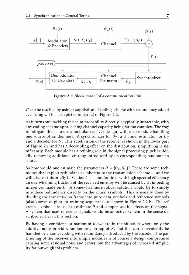
Digital communication systems are heavily dependent on synchronization for ef-fective operation. To illustrate why, we will use a common model with one trans-mitter unit sending a digital message over a waveform channel to a receiver unit.The transmitter includes a modulator that maps bits X[n] onto a continuous wave-form S(t, X; θT ), where the stochastic process θT (t) represents the timing andfrequency state of the modulator. The channel filters S according to the channelfunction h(S; θC) and stochastic channel state θC(t). Finally, there is noise N (t)added to the received waveform. This is depicted in Figure 2.1.
The task of the receiver is to map the received signal Y (t, S; θC , N ) = h(S; θC) +N (t) back to data bit estimates X̂[n] as accurately as possible. If the transmit-ter design and channel statistics are completely known, all uncertainty can beexpressed as a joint probability p(X, θT , θC , N ) and the channel capacity3 C isgiven as
C = suppX (x)
I(X; Y ). (2.1)
3In this thesis, channel capacity refers to the theoretical maximal achievable information rate overa channel and cell capacity to the maximal number of simultaneous users a cell can serve.
2.1 Synchronization in General Terms 7
Modulator(& Encoder)
θT (t)
Channel
θC(t)
+
N (t)
SynchronizerChannelEstimator
Demodulator(& Decoder)
Receiver
X[n] S(t, X; θT ) h(t, S; θC)
Y (t)
θ̂Tθ̂T , θ̂CX̂[n]
Figure 2.1: Block model of a communication link
C can be reached by using a sophisticated coding scheme with redundancy addedaccordingly. This is depicted in part a) of Figure 2.2.
As it turns out, tackling this joint probability directly is typically intractable, withany coding scheme approaching channel capacity being far too complex. The wayto mitigate this is to use a modular receiver design, with each module handlingone source of randomness. A synchronizer for θT , a channel estimator for θCand a decoder for N . This subdivision of the receiver is shown in the lower partof Figure 2.1 and has a decoupling effect on the distribution, simplifying it sig-nificantly. Each module has a refining role in the signal processing pipeline, ide-ally removing additional entropy introduced by its corresponding randomnesssource.
So how would one estimate the parameters θ = {θT , θC}? There are some tech-niques that exploit redundancies inherent to the transmission scheme — and wewill discuss this briefly in Section 2.4 — but for links with high spectral efficiency,an overwhelming fraction of the received entropy will be caused by X, impedinginferences made on θ. A somewhat more robust solution would be to simplyintroduce redundancy directly on the actual symbols. This is usually done bydividing the transmission frame into pure data symbols and reference symbols(also known as pilot- or training sequences), as shown in Figure 2.2 b). The ref-erence symbols are used to estimate θ and compensate its effects on the signal.A system that uses reference signals would be an active system in the sense de-scribed earlier in this section.
By having a confident estimation of θ, we are in the situation where only theadditive noise provides randomness on top of X, and this can conveniently behandled by channel coding with redundancy introduced by the encoder. The par-titioning of the receiver into simple modules is of course a design compromisecausing some residual noise and errors, but the advantages of increased simplic-ity far outweigh this problem.

8 2 Synchronization in OFDM Systems
Data Bits Parity Bitsa)
DataBits
ParityBits
ChannelPilots
SynchronizationPilots
b)
Figure 2.2: Frame structure using: a) optimal codec b) modular design
Replacing data symbols by pilots will reduce the immediate data rate, but alsoreduce the error rate, which means less redundancy requirements in the codec.Instead of being set by theoretical calculations, the pilot rate is usually set by con-sidering the specific application at hand and its specific requirements on through-put, latency and reliability. In the next section, we will describe the modulation-and multiplexing scheme used in nb-iot in order to enable more detailed discus-sions regarding synchronization schemes.
2.2 Orthogonal Frequency-Division Multiplexing
Many modern high-data-rate wireless communication systems — including nb-iot, Long-Term Evolution (lte) and WiFi — are based on orthogonal frequency-division multiplexing (ofdm). ofdm is a scheme for modulation and multiplex-ing of digital data, hence, the usage of ofdm has important implications on syn-chronization design.
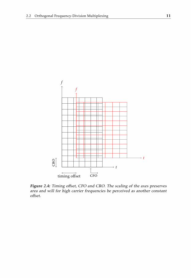
The idea of ofdm is to use a relatively low symbol rate and then do quadratureamplitude modulation (qam) on the harmonics of the symbol rate coherently. Bydoing this, one effectively get frequency division multiplexing with orthogonalsubcarriers. Since the harmonics are integer multiples of the symbol rate there isa constant subcarrier spacing, which creates a rectangular two-dimensional gridof resources, delimited by symbol time on one axis and its inverse (subcarrierspacing) on the other. Every point on the grid can hold one qam symbol, whichcreates an opportunity to schedule data transmissions in both time and frequency.Figure 2.4 illustrates time-frequency grids.
By keeping the symbol rate low, the channel delay spread will not destroy thesymbol completely, and we can even afford a guard interval on each symbol toprevent intersymbol interference (isi). The most common way to allocate theguard interval is to use a so called cyclic prefix (cp) where the last samples areextended cyclically to prefix the symbol. Another way of interpreting the lowsymbol rate is as a low subcarrier spacing, effectively creating a set of channelswith a bandwidth narrow enough to experience flat fading. This is a main reasonfor ofdm being widely used in fading wireless environments. The maximumbandwidth under which the channel can practically be considered flat is calledcoherence bandwidth and is approximately proportional to the delay spread. Allthe different parameters defining the ofdm waveform — including subcarrier

2.2 Orthogonal Frequency-Division Multiplexing 9
spacing, cp length and larger scale structures for allocation of resources — canbe set in a variety of ways. A specific setting of these parameters is called anumerology4.
As it turns out, the scheme described above is equivalent to a Fourier series. Thefact that a sampled Fourier series is equal to an inverse discrete Fourier trans-form of the same coefficients enables a convenient digital implementation of thebaseband modulation. The demodulation procedure can similarly be based ona discrete Fourier transform, complemented by the usual downconversion andsymbol detection used in a qam system. A simplified view of an ofdm receivercan be seen in Figure 2.3.
Figure 2.3: OFDM demodulator with local oscillator (fc) and sample clock(fs) separated. [Source: Wikimedia Commons (remix)]
2.2.1 OFDM Synchronization Tasks
Even though ofdm is a compelling scheme for fading channels, it is largely de-pendent on accurate synchronization. The effects of deficient synchronization arediscussed in Section 2.2.2. But first, the main tasks required for synchronizationin ofdm are described.
Symbol and frame timing
To demodulate a received signal into symbols, the receiver needs to know thesymbol timing, i.e. the time instance marking the start of a new symbol. Oth-erwise, the information of one symbol will distort the demodulating of another,causing isi. Due to the lack of an exact common time reference (and the unknowntime delay), the symbol timing information has to be extracted from the signalitself.
In addition, the receiver also needs information on which symbol constitutes thestart of a new frame. Since transmission schemes typically employ a hierarchicalframing structure with multiple types of data, the index of the symbol markinga complete frame period (i.e. the frame timing) must be known.
4Not to be confused with mystical beliefs.

10 2 Synchronization in OFDM Systems
Carrier Frequency Offset
Similarly to timing, also frequency information has to be learned. Assumingprior knowledge in the receiver of the carrier frequency the transmitter intendto use, fc, there might still be a frequency discrepancy due to Doppler shift andto local oscillator instability on both sides. This is called carrier frequency offset(cfo). With c being the speed of light, d the distance between the units and LOT xand LORx the local oscillator frequency errors (usually expressed in ppm) of thetransmitter and receiver respectively, the aggregate cfo effect will be given as thescaling factor
φ =1 + LOT x1 + LORx
· cc + d′
. (2.2)
This scaling can be interpreted as an area-preserving scaling of the axes in thetime-frequency grid, illustrated by Figure 2.4. This factor is usually very smalland have a negligible effect on a single symbol. However, cfo will affect thedown-conversion, leading to a baseband frequency shift proportional to fc, andfc is often much larger than the bandwidth. This frequency shift will cause inter-carrier interference (ici) that reduces carrier orthogonality. Also, time-drift willadd up over many symbols, again causing isi.
Note that the effect we describe here is usually more accurately ascribed to thesampling clock error. We assume here that the sampling frequency, fs, and localoscillator frequency, fc, originate from the same source and abuse the term cfo(as commonly done in literature). Pure frequency offset will instead be referredto as carrier raster offset (cro).
Carrier Raster Offset
Prior knowledge of fc will not always be complete. For synchronization to befeasible, the prior knowledge should include a reasonably small set of frequenciesto search through: a search raster. By searching through this raster, one shouldbe guaranteed to hit the correct frequency only by a small error, the cro. Thecro has the effect on an actual offset, i.e. a shift in frequency.
While cfo causes time drift, cro does not. But synchronization schemes aretypically designed to correct the total perceived frequency error fe = cfo + cro.This leads to a problem when compensating for time drift. If for example cfo >>cro, the system can assume the time drift being proportional to fe and the crowill then lead to a residual time-drift due to overcompensation.
Channel estimation and equalization
As described in Section 2.1.1, channel estimation and equalization may be doneafter synchronization. This procedure is in some sense analogous to synchro-nization, with channel reference symbols providing redundancy for parameterestimation. Channel coherence time is defined as the maximum time period un-der which the channel can practically be considered time-invariant. By doing achannel estimation at an interval considerably smaller than the channel coher-
2.2 Orthogonal Frequency-Division Multiplexing 11
t
f
t
f
timing offset
cro
cfo
Figure 2.4: Timing offset, CFO and CRO. The scaling of the axes preservesarea and will for high carrier frequencies be perceived as another constantoffset.

12 2 Synchronization in OFDM Systems
ence time, the coding scheme will not need to cover up for any entropy inducedon the received signal by the channel dynamics.
One important issue that we have not yet mentioned is that of carrier phase,which can vary due to instabilities in the transmitter or receiver oscillators. Wewill consider this effect as part of the channel and leave the equalizer to compen-sate for the effect.
2.2.2 Effects of Deficient Synchronization
We have mentioned synchronization tasks, with the most important effects beingisi and ici. These are obviously to be avoided and we will here give an exampleof how their effects can be quantified. The effects are measured by how much theperceived snr gets affected.
Note that in many multi-user systems, ofdm is used for multiple access, thusthe effects of poor synchronization of one user are not only degrading its perfor-mance, but also affecting other users, which is called multiple-access interference(mai). In this case, synchronization is not only a matter of increasing channelcapacity for ones own link, which makes the discussions in Section 2.1.1 aboutredundancy rather more complicated.
OFDM Timing errors
snr loss, γ , can be calculated as a function of the timing error, ∆τ , from fourquantities: signal power E{|S(t)|2}; noise power σ2
N ; interference from isi and ici,modeled as a zero-mean variable with variance σ2
I (∆τ); and an attenuation factor,α2(∆τ), representing the fact that part of the signal will be outside the samplingwindow. By assuming that the channel and frequency is known, and normalizingthe channel impulse, we get [4] that
γ(∆τ) :=snr(ideal)
snr(real)=
E
{|S(t)|2
}/σ2N
E
{|S(t)|2
}α2(∆τ)/[σ2
N + σ2I (∆τ)]
=1
α2(∆τ)
[1 +
σ2I (∆τ)
σ2N
].
(2.3)
OFDM Frequency errors
Similarly, when the channel and timing is known, the snr loss can be calculatedfrom the frequency error, ε, as follows. By normalizing the channel impulse, wehave [4]
γ(ε) :=snr(ideal)
snr(real)=
1
|fn(ε)|2
1 +E
{|S(t)|2
}σ2N
[1 − |fn(ε)|2]
≈ 1 +E
{|S(t)|2
}3σ2
N
(πε)2
(2.4)
2.3 Cellular OFDM and Initial Cell Search 13
where n is the number of available subcarriers and
fn(ε) =sin(πε)
n sin(πε/n)ejπε(n−1)/n. (2.5)
2.3 Cellular OFDM and Initial Cell Search
In cellular networks, connectivity is provided to all user equipments (ues) in acell by a base station (bs). Transmission from bs to ue is referred to as downlink(dl) and the opposite direction is called uplink (ul). The bs often coordinatesand schedules traffic for a large number of ues within the cell and makes surethat they communicate efficiently with users or networks outside the cell. It istherefore appropriate to have each ue adapt to the rest of the system, with the bsacting as a centralized source of timing by providing dl reference symbols.
The dl synchronization will provide everything the ue needs for reception, butdue to Doppler shift and time delay, ulwill still suffer frommai, unless some ulsynchronization takes place. After dl synchronization, the mai can be resolvedeither by sophisticated signal processing at the bs, or by providing feedback ofDoppler shift and time delay on the dl, to have the ue compensate.
When a new ue wants to connect to a cell, it first needs to detect the cell andany specific system information before attempting to connect. It is also impor-tant that coarse synchronization happens on dl before ul, to minimize the maicaused by the ue. This first procedure is called cell acquisition or initial cellsearch (ics). After ics is done, the ue can move on to the random access proce-dure. When successful communication has started, the ue needs to do fine syn-chronization continuously, referred to as tracking. Tracking can be based uponadaptive signal processing techniques but may also rely on the same algorithmused for ics. We will only treat ics. Following is an exemplary outline of the icsprocedure:
1. The ue powers on.
2. Check SIM-card for band or raster information.
3. Scan entire raster for cell power profile.
4. Try to synchronize on loud candidate frequencies:
a) Frame or symbol timing (our main focus)
b) Frequency estimation
c) Frame numbering
d) Channel and phase estimation
e) Cell ID and system information
5. Do random access procedure (with ul synchronization).
6. Request scheduling.

14 2 Synchronization in OFDM Systems
7. Start communication and do tracking continuously.
2.4 OFDM Downlink Methods
The core part of timing and frequency synchronization consists of two steps. Thefirst could simply be stated as the estimation of shift in time and frequency of thedl signal. As we know from Fourier analysis, a shift in one domain correspondsto a rotation in the other. Consequently, this step can be done by estimating shift,rotation or a combination of both. The general problem, given received signal Y ,can be expressed as
(t̂, f̂ ) = argmax(t,f )
L1(Y , t, f ) (2.6)
where the cost function L1 ideally should be based on high level metrics suchas minimization of pst or maximization of perceived snr, but will in practicalcases be based on common parameter estimators like maximum likelihood orlinear minimum mean squared error, or on other heuristics. Figure 2.5 illustratesan example of an estimation metric as a function of timing error.
−4 −3 −2 −1 0 1 2 3 40
2
4
6
8
10
12
Timing error [ofdm symbols]
Tim
ing
met
ric,L
1
Figure 2.5: Example of a timing metric. The data is taken from the prestudyand the cost function is |ρ| (defined in the next chapter).
The second part is a matter of detection. Due to factors such as power consump-tion and mai, it may not be worthwhile to attempt communication unless theprevious estimation is accurate enough. Thus there should be some detection
2.4 OFDM Downlink Methods 15
threshold, λ, determining whether the dl signal estimation is confident enough.The confidence metric, L2, will typically be a function of a subset of L1 and itsderivatives:
L2
({∂m+nL1
∂tm ∂f n
})≶ λ (2.7)
Detection is often treated quite easily by adjusting λ to some given target far.The more intricate problem is that of estimation. The estimation in equation (2.6)can be simplified if the time can be decoupled from frequency. This is analogousto the modular receiver design but take it one step further, and similarly sufferfrom some loss in maximal achievable performance. This cost of this loss could bemade insignificant in comparison with the reduced cost by the much less complexdesign.
Pilot-free approaches
We mentioned earlier that synchronization methods may or may not be based onpilot signals. Pilot-free methods need to exploit some characteristic of the wave-form design. Examples of this include searching for power profiles or utilizingsilent periods such as guard intervals. Utilization of recurring silence imply a re-liance on a constant stream of data packets or other statically allocated symbolsto be transmitted, which may not always be provided. Other pilot free methodsexist, for example utilizing redundancy in the cp of ofdm, which is often sig-nificantly longer than delay spread and therefore carries some redundancy. Thepitfalls of this method are several: it also relies on continuous transmissions; thecp is only a fraction of a symbol, thus providing only a small snr gain; occasionallong channel delay spreads may impede potential gains from this method. Pilot-free methods have been shown to perform at an unsatisfactorily low accuracy[4].
The acquisition procedure, as outlined in Section 2.3, consists of several steps ofincreasing granularity. Pilot-free methods may have a place early in this process,where a crude measurement such as received signal strength indication can pro-vide guidance. So the more compelling alternative is to use pilot-based methods.There are different varieties of these and some are introduced below for specificphases of the synchronization procedure.
Coarse timing
Since, inofdm systems, timing estimation is typically the first thing that happens(Section 2.3), any timing method should be robust enough to handle a relativelylarge cfo. It should also be robust to the unknown channel. While very precisetiming can be hard to achieve at this stage, a coarse estimate is easier. The coarsetiming estimate can be used to do frequency synchronization before a fine timingis finally done. The distortion caused by the cfo and the channel can make it un-fruitful to do cross-correlation of the received signal with a memorized copy ofthe pilot. One solution to this is to use as pilot a sequence, B, duplicated in time,and instead detect it by a sliding auto-correlation window [5]. If each copy of B is

16 2 Synchronization in OFDM Systems
much longer than the delay spread (as should be guaranteed by the cp), the chan-nel distortion on each copy, B, should be similar, yielding only a negligible effecton the auto-correlation. The effect of the cfo will be a complex time rotation onthe signal, which by using auto-correlation will be seen as nothing but a complexrotation between the symbols. The magnitude of the sliding auto-correlation willpeak when the window matches the pilot, if the pilot is large enough to prohibitrandom data from creating false alarms. A refined version of this uses more thantwo copies, [B, B, −B, B], to sharpen the peak [6]. The binary sequence of copiesis called code cover in this thesis. What constitutes a good code cover will bediscussed later.
Fine timing and tracking
At the end of the ics procedure, more accurate timing can be achieved for ex-ample by using a higher sampling rate. Sub-sample level accuracy can be in-corporated into the channel estimate. Due to oscillator instabilities and varyingDoppler shift — but more importantly, residual time drift — the fine timing thenhas to be tracked. The time drift can be captured explicitly by tracking the vary-ing time delay of the channel impulse response maximal taps [4].
Frequency acquisition
Many methods for frequency acquisition in principle rely on measuring the cfoinduced phase shift between symbols. Since phase is periodic, only the phaseshift modulo 2π can be measured. This is equivalent to determine the frequencyoffset from the nearest sub-carrier and is called fractional frequency estimation.To get a complete frequency estimate the correct subcarrier must be found, whichis called integer frequency. Finding the fractional frequency is by nature a con-tinuous problem, while integer frequency can be found by hypothesis testing ona number of plausible subcarriers. [4]
An example of how fractional frequency can be found is given by the previouslydescribed timing method that uses two copies of B [5]. Here, the phase betweenthe copies is utilized. In the same paper, a method is described for finding integerfrequency by using an extended reference sequence, [B, B, P1, P2], where P1 andP2 are pseudo-noise reference sequences. After fractional frequency is found andcompensated for, a discrete Fourier transform of the signal is done followed bya cross-correlation in frequency domain with memorized copies of P1 and P2. Inthis way, the integer frequency can be found. A similar approach using a smalleroverhead is introduced in [7]. This technique is part of the synchronization algo-rithm used in this study.
Frequency tracking
The need for frequency tracking stems from same reason as we do time track-ing. Usually, it suffices to repeat the acquisition procedure. Other classical ap-proaches that are used for this are based upon phase-locked loops, which can bedeployed using error signals in time or frequency domain.

2.4 OFDM Downlink Methods 17
2.4.1 Pilot Characteristics
How should one choose the B from the earlier part? This question is centralto both synchronization design generally and also to this thesis specifically. Asmentioned earlier, synchronization corresponds to estimating shift or rotation intime and frequency. Shifts are found by correlation, which requires sequenceswith good auto-correlation properties, i.e. a sharp peak at zero and low side-lobes for non-zero shifts of the auto-correlation function. Rotations converselyare easily found on sequences with nearly constant amplitude. Not surprisingly,constant amplitude translates to the described good auto-correlation propertiesby Fourier transform. Thus, for pilot sequences to facilitate synchronization oftime and frequency, they need to have zero auto-correlation and constant ampli-tude in both domains. Such sequences are called constant amplitude zero auto-correlation waveform (cazac).

3Narrowband Internet of Things
With the previous chapter introducing some aspects of synchronization for ofdmsystems, we will now have a look at what this means for Narrowband Internet ofThings. This chapter will introduce the purpose and capabilities of nb-iot aswell as its design features and limitations relevant to our study. The first sectionexpands on Chapter 1 and gives a background of the motivation for creatingnb-iot. It is followed by a short description of parts of the air interface, withemphasis of features relevant to synchronization. We will then describe in detailhow the synchronization system of nb-iot is designed and it how it relates to theconcepts in the previous chapter, encompassing both the transmitter and receiverside of the dl.
3.1 LTE, 5G and mMTC
Cellular communication is an example of a technology that has been very suc-cessful in the last decades, with recent standards such as lte enabling the out-standing use today of hundreds of millions of smartphones with services suchas high-definition video calls between continents. In the coming years however,the number of connected devices as well as the number of use cases is expectedto increase massively, much driven by so called machine type communication(mtc). This requires a continuous fast paced research and development of wire-less networks, as today’s (although capable) networks will be insufficient in a fewyears.
There is a widespread consensus within the telecom industry that the 5th Gen-eration Mobile Networks (5g) devices can suitably be divided into three majorkinds of applications. These were defined [1] by International Telecommuni-
19

20 3 Narrowband Internet of Things
cation Union (itu) as being: enhanced mobile broadband , which is the natu-ral improvement of today’s mobile broadband with higher data rates support-ing video streaming and virtual reality; massive machine type communication(mmtc), which refers to a large quantity of low-end devices such as sensor- andactuator networks, meters (water, gas, electric, or parking), home automation,etc; and ultra-reliable low latency communications which refers to highly criticallinks for applications such as remote surgery, vehicular communication systemsand cloud-based control of drones and robots. Their requirements are summa-rized in Figure 3.1.
Figure 3.1: The importance of key capabilities in different usage scenarios.[Source: IMT Vision, ITU]
Part of 3gpps 5g transition strategy includes a new radio interface called 5g NewRadio, which presumably will meet all the requirements of 5g. The details of thisdevelopment are not yet clear, but what is certain is that the transition to 5g willdepend on deployments of 5g New Radio in tandem with extensions of lte (asof now called lte Advanced Pro or 4.5G).
This thesis concerns only the mmtc part of 5g. lte has been developed primarilywith mobile broadband in mind, and only to some extent for mtc. Recent workby 3gpp for mtc include EC-GSM-IoT and the lte-mtc1 cost reductions intro-duced in release 13. To more convincingly meet the needs of 5g mmtc, a newtechnology was introduced in release 13, namely nb-iot, with commercial prod-ucts already on the market as of early 2017. nb-iot is somewhat based on lte,sharing the numerologies for the ofdm dl, as well as tail-biting convolutionalcodes with interleaving and rate matching from lte [8]. The design, however, ismodified and streamlined to meet the following requirements [9]:
• High cell capacity: >52 500 devices
• Low cost: <$5 per device1Also known as LTE-M or eMTC, but more formally referred to as LTE CatM1/M2
3.2 Downlink Physical Layer 21
• Low power consumption: >10 years with a 5 Wh battery
• Improved coverage: 20 dB better than gsm2
• Relaxed device data rate requirements
• Relaxed latency requirements
3.2 Downlink Physical Layer
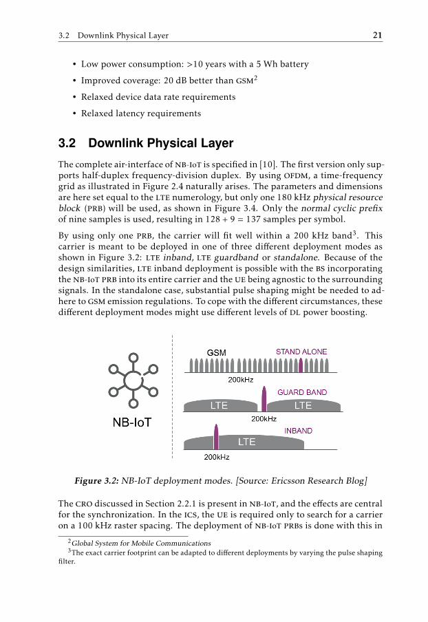
The complete air-interface ofnb-iot is specified in [10]. The first version only sup-ports half-duplex frequency-division duplex. By using ofdm, a time-frequencygrid as illustrated in Figure 2.4 naturally arises. The parameters and dimensionsare here set equal to the lte numerology, but only one 180 kHz physical resourceblock (prb) will be used, as shown in Figure 3.4. Only the normal cyclic prefixof nine samples is used, resulting in 128 + 9 = 137 samples per symbol.
By using only one prb, the carrier will fit well within a 200 kHz band3. Thiscarrier is meant to be deployed in one of three different deployment modes asshown in Figure 3.2: lte inband, lte guardband or standalone. Because of thedesign similarities, lte inband deployment is possible with the bs incorporatingthenb-iot prb into its entire carrier and the ue being agnostic to the surroundingsignals. In the standalone case, substantial pulse shaping might be needed to ad-here to gsm emission regulations. To cope with the different circumstances, thesedifferent deployment modes might use different levels of dl power boosting.
Figure 3.2: NB-IoT deployment modes. [Source: Ericsson Research Blog]
The cro discussed in Section 2.2.1 is present in nb-iot, and the effects are centralfor the synchronization. In the ics, the ue is required only to search for a carrieron a 100 kHz raster spacing. The deployment of nb-iot prbs is done with this in
2Global System for Mobile Communications3The exact carrier footprint can be adapted to different deployments by varying the pulse shaping
filter.

22 3 Narrowband Internet of Things
Table 3.1: nb-iot physical channels and signals.
Channel Main purposes
Broadcast channel System information, frame numberControl channel Scheduling, acknowledgements, paging, etcShared channel Higher level payload data, etcReference signals Demodulation phase referencenpss Frame boundary, frequencynsss Frame number, cell ID
mind. For inband and guardband deployments however, the prbmust be alignedwithin the lte grid. By deploying nb-iot on a wisely chosen subset of lte prbs,the nb-iot carrier can be placed ±2.5 kHz or ±7.5 kHz from nearest frequencyraster point (i.e. a multiple of 100 kHz). For standalone deployments, the prbcan be placed exactly on the raster. The prior offset uncertainty in the ue of upto 7.5 kHz constitutes the cro.
3.2.1 Physical Channels and Signals
In 3gpp standards, a physical channel is a set of physical resources in the time-frequency grid dedicated for transmission of some specific information, withspecifications on the transmission format. In nb-iot, the physical channels arebased on an essential subset of the lte physical channels. An initial capital Nhave been added to their abbreviations to emphasize that they are specific tonb-iot. Even though the physical channel specifications are changed from lte,their respective purposes remain mostly unchanged, as summarized in Table 3.1.As we will see, this thesis concerns only the synchronization signals of nb-iot:npss (Narrowband Primary Synchronization Signal ) and nsss (Narrowband Sec-ondary Synchronization Signal ) — primarily4 npss.
even numbered frame odd numbered frame
subframe = 1 ms
npss
nsss Broadcast channel
Payload or control data
Figure 3.3: NB-IoT frame structure
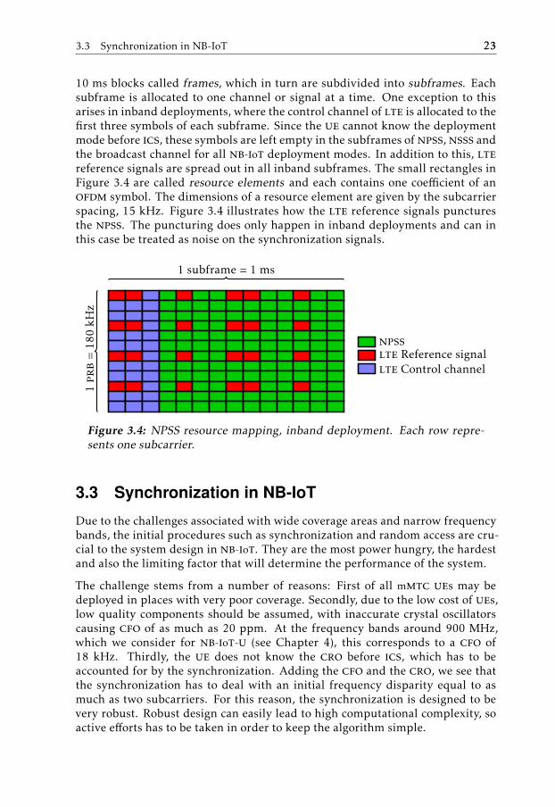
Figure 3.3 illustrates the basic time-domain structure. Time is divided up into
4No pun intended.
3.3 Synchronization in NB-IoT 23
10 ms blocks called frames, which in turn are subdivided into subframes. Eachsubframe is allocated to one channel or signal at a time. One exception to thisarises in inband deployments, where the control channel of lte is allocated to thefirst three symbols of each subframe. Since the ue cannot know the deploymentmode before ics, these symbols are left empty in the subframes of npss, nsss andthe broadcast channel for all nb-iot deployment modes. In addition to this, ltereference signals are spread out in all inband subframes. The small rectangles inFigure 3.4 are called resource elements and each contains one coefficient of anofdm symbol. The dimensions of a resource element are given by the subcarrierspacing, 15 kHz. Figure 3.4 illustrates how the lte reference signals puncturesthe npss. The puncturing does only happen in inband deployments and can inthis case be treated as noise on the synchronization signals.
1 subframe = 1 ms
1prb
=18
0kH
z
npsslte Reference signallte Control channel
Figure 3.4: NPSS resource mapping, inband deployment. Each row repre-sents one subcarrier.
3.3 Synchronization in NB-IoT
Due to the challenges associated with wide coverage areas and narrow frequencybands, the initial procedures such as synchronization and random access are cru-cial to the system design in nb-iot. They are the most power hungry, the hardestand also the limiting factor that will determine the performance of the system.
The challenge stems from a number of reasons: First of all mmtc ues may bedeployed in places with very poor coverage. Secondly, due to the low cost of ues,low quality components should be assumed, with inaccurate crystal oscillatorscausing cfo of as much as 20 ppm. At the frequency bands around 900 MHz,which we consider for nb-iot-u (see Chapter 4), this corresponds to a cfo of18 kHz. Thirdly, the ue does not know the cro before ics, which has to beaccounted for by the synchronization. Adding the cfo and the cro, we see thatthe synchronization has to deal with an initial frequency disparity equal to asmuch as two subcarriers. For this reason, the synchronization is designed to bevery robust. Robust design can easily lead to high computational complexity, soactive efforts has to be taken in order to keep the algorithm simple.

24 3 Narrowband Internet of Things
As mentioned earlier, both npss and nsss take up one subframe. The actualsignals are composed of sophisticated sequences. The npss has a hierarchicalstructure, consisting of a base sequence and a code cover. This structure is crucialfor our study and will be described below.
3.3.1 Base Sequence
Wireless communication standards are full of reference signals of different kindsand many of them are cazac. One such type of sequences that have seen suc-cessful use in the third and fourth generation wireless technology is Zadoff-Chusequences [11]. They are defined as
du(n) = exp(−jπun(n + 1 + 2q)
NZC
)(3.1)
where the parameter u is called root index, q is the shift of the sequence and NZCis the length of the sequence. In nb-iot, the parameters are set to q = 0, u = 5 andNZC = 11. The length-11 sequence is mapped to each ofdm symbol of the npss.So if there are twelwe subcarriers, why not use NZC = 12? The answer comesfrom the fact that if NZC is prime, then the time-domain sequence will also beZadoff-Chu, and as it turns out also periodic and symmetric. Periodicity allowsfor smoother time-domain concatenation of the ofdm symbols and the symmetrycan be exploited for cheaper receiver signal processing.
As can be seen from n appearing twice in the equation (3.1), the sequence is chirp-like (i.e. having an increasing rate of change), which is related to it being cazac.One good reason Zadoff-Chu sequences has been used in many standards is thatthe cross-correlation is zero for sequences of different shifts, q, and constant fordifferent roots, u. For nb-iot, the important aspect is not the auto-correlationitself, but the fact that it has constant amplitude in time (improving the cubicmetric) and frequency domain (limiting spurious emissions).
3.3.2 Code Cover
The second layer of the npss structure is the code cover. It is the same kind ofcode cover that is described in Section 2.4, with B here being the base sequence.Each npss ofdm symbol consists of B or −B, as shown in Figure 3.5. The npsscode cover is ([2])
s = [+ + + + − − + + + − +], (3.2)
so the npss block, H , in Figure 3.5 can be expressed as
Hn,k = d5(n) · s(k), (3.3)
where n and k index rows and columns respectively.
3.3.3 Reciever NPSS Processing
Regardless of its properties, the performance of a particular npss will only be asgood as the ues ability to process it. Therefore, the npss we described here, was

3.3 Synchronization in NB-IoT 25
1 subframe = 1 ms
1prb
=18
0kH
z
+ Zadoff-Chu− Zadoff-ChuEmpty
Figure 3.5: NB-IoT NPSS structure, standalone deployment.
proposed to 3gpp together with a corresponding receiver algorithm [12]. Thecombination of the signal and the algorithm was shown to be robust and com-putationally cheap [12]. The algorithm used in this report is based on this 3gppcontribution and its revisited version [2], with only minor changes.
The principles behind the algorithm are based upon methods we described inChapter 2. Timing estimation is done akin to [6] and the frequency estimationdone akin to [7]. These techniques are in this algorithm combined using a singlemetric function for timing and frequency. The signal processing steps of thealgorithm are outlined below, similarly to the description in [2].
1. Downsampling
The standard sampling frequency in nb-iot is 1.92 MHz, but the npss processinguses a reduced sampling rate of 240 kHz, for computational simplicity. The algo-rithm will process one 10 ms frame at a time and try to find among the samplesτ ∈ [1, 2, . . . , 2400], the sample, τ0, where the npss starts.
2. Autocorrelation
For each new sample, τ , the vector r(τ) = [r1(τ), r2(τ), . . . , rK (τ)] is formed fromthe most recent samples5. K is the length of the code cover. K = 11 for nb-iot.Each ri(τ) has the length of one symbol and r(τ) the length of thenpss. For τ = τ0,r(τ) will match the npss, a fact that is the basis for the following processing. Thefirst step is to reapply the code cover, s, and do cross-correlation between thesymbols:
Ak(τ) =1
K − k
K−k∑m=1
(s(m + k) rm+k(τ)) (s(m) rm(τ))H , k = 0, 1, 2, 3, 4 (3.4)
k is limited to 4 to keep processing complexity low. Thanks to auto-correlationproperties of s, the magnitude of Ak(τ) will peak for τ = τ0. To see this, note thatfor τ = τ0, the reapplication of s will produce a sequence of K identical symbols
5Note that samples from the previous frame might be needed.

26 3 Narrowband Internet of Things
(not counting channel effects and noise), while for other values of τ , the codecover will not match the signal and instead create a new pseudo-random pattern.When τ = τ0, the cfo induced phase rotation, θ, between adjacent symbols willbe given by
E {Ak(τ0)} ∝ ejkθ . (3.5)
Thus, timing and frequency can be extracted from the magnitude and phase ofAk(τ) respectively. This is the basis for the entire algorithm.
3. Exponential smoothing
Recall that the snr might be very poor, so Ak(τ) is too noisy to provide reliableestimates. For this reason, the synchronization algorithm utilizes the retransmis-sions of the npss to do accumulation over several frames
Ak(τ)n B α · Ak(τ)n−1 + (1 − α) · Ak(τ) (3.6)
where n denotes the current frame number and the bar notation indicates theaccumulation operation defined by the equation. The forgetting factor, α, is ad-justed to the expected time-drift of the system, as explained in Section 5.1.
4. Coherent combining
The next step is to extract the actual metric,
ρ(τ) B3∑k=0
wkAk+1(τ)Ak(τ)∗
(3.7)
where wk are fixed weights that were set for minimum mean squared error in thisstudy. Notice the similarity with equation (3.4). This step can be seen as coherentcombining at a higher level. Thus, timing and frequency is still contained inthe complex value ρ(τ), but with better accuracy than in Ak(τ). The accuracy ofρ(τ) is expected to increase for every new frame due to the accumulation in theprevious step. The next step in the processing is to decide when the estimate isaccurate enough. Either 5a or 5b can be used for this decision.
5a. Peak detection
The metric, ρ(τ), is expected to have a large magnitude for τ = τ0. If the magni-tude has a large peak for some τ , the estimate is likely to be accurate. With
(ρmax, τ̂) = maxτ
{|ρ(τ)|∑i |ρ(i)|
}, (3.8)
τ̂ can be used as timing estimate if ρmax > λP . Otherwise the accumulation pro-cedure should continue. λP is called the Peak detection threshold and should beset to balance pst and far.
5b. Genie detection
When evaluating the estimation performance of different synchronization schemes,the false alarms can make the comparison more complicated. One way to deal
3.3 Synchronization in NB-IoT 27
with this is to get rid of the detection problem by using a detection rule herereferred to as Genie detection. It works as follows: τ̂ is used as timing estimateif |τ̂ − τ0| < λG, otherwise the accumulation procedure should continue. λG iscalled the Genie detection threshold, and the name stems from the fact that thereceiver needs to magically know τ0 to do the detection. This rule is impossibleto implement in a ue and is only used for the simulation.
6. Fractional frequency
When the timing is estimated, a fractional frequency estimate, f̂F , can be acquiredaccording the principle in equation (3.5). The estimate is given by
f̂F B128137·
arg{ρ(τ̂)
}2π
, (3.9)
where the first factor compensates for the length-9 cp.
7. Integer frequency
The integer frequency estimate, f̂I , can be acquired by hypothesis testing over thesubcarriers that are reasonable, given the maximum cfo and cro in the systemmodel. With a 20 ppm cfo at 900 MHz and a cro of up to 7.5 kHz for example,the maximum integer frequency offset is limited to two subcarriers. The estimateis given as
f̂I B128137
argmaxfI∈{±2,±1,0}
Cr,npss(τ̂ , f̂F +128137
fI ), (3.10)
where Cr,npss denotes cross-correlation of r(τ̂) counter-phase rotated accordingto f̂F + 128
137 fI , with a copy of the npss.
3.3.4 Receiver NSSS Processing
The nsss is also based upon Zadoff-Chu sequences, but with different root in-dices, and is scrambled according to one of several predefined binary sequences.The root index and the index of the scrambling pattern can encode digital infor-mation. The cell ID is encoded, together with the last three significant bits ofthe current frame number [8]. Thus, timing can be achieved within a windowof eight frames, or 80 ms. The nsss can also be used to refine the fractional fre-quency estimation by correlation in the frequency domain at the higher samplingrate of 1.92 MHz. nsss processing is much easier than npss processing, and wasnot investigated in detail in this study. Instead, an off-the-shelf algorithm alreadyimplemented in the simulator was used.
3.3.5 Master Information Block
The remaining four bits of the frame number are bundled together with othersystem information and transmitted in the broadcast channel as a packet calledmaster information block (mib). Themib is divided up into eight subblocks, eachof which is repeated in every first subframe of eight consecutive frames (see Fig-

28 3 Narrowband Internet of Things
ure 3.3). Thus it takes 640 ms to transmit one mib before any new system infor-mation can be transmitted.
4Operation in Unlicensed Spectrum
Initial standardization of nb-iot has been completed and user chip-sets are al-ready available as of 2017. Like for many other wireless standards, nb-iot willlikely be updated to enable more features or improve on previous ones. One ma-jor theme in 5g research is the migration of cellular systems into new frequencybands. This includes exploiting the very wide millimeter-wave bands as well asrefarming bands that was previously used for services that are now obsolete1. Athird kind is the migration into unlicensed bands, which entail a new set of de-sign challenges brought by the specific regulations in these bands. The challengesassociated withnb-iot-u— adaption ofnb-iot into unlicensed spectrum — is themain motivation for this thesis. This chapter will first provide a brief introduc-tion to these bands and why they are useful, adding to the motivation providedin Section 1.1. This chapter then introduces the most suitable frequency bandsfor nb-iot-u and what limitations their regulations impose on synchronization.
4.1 Frequency Bands
Regulation and administration of the radio spectrum is done to various degreesand in various ways globally (by itu), regionally (e.g. by Electronic Communi-cations Committee (ecc) in the EU) and nationally (e.g. by Federal Communi-cations Commission (fcc) in the U.S.). This process is quite complicated, withmany participating organizations. The role of global and regional organizationsis to set standards and provide guidelines to be followed by individual nations,but in the end the radio spectrum is actually regulated by national governmentagencies. They divide the spectrum into bands and decide who can use each band,
1The nb-iot standalone deployment mode is an example of refarming gsm bands.
29

30 4 Operation in Unlicensed Spectrum
for what purpose and under which conditions. [13, Chapter 2]
Bands used for civil communication systems can either be licensed or unlicensed.Licensed bands are bands that require a license for operation. A license usuallyentails the sole right of operation in a specific band and is made available by agovernment agency through auctioning. With a licensed band an operator canthus have full control over the interference within the band, enabling very effi-cient multiple access and coordination schemes. The auction price per usefulMHz in the U.S. have been on the order of hundreds of millions of dollars in thelast decades.
Unlicensed bands on the other hand are open for anyone to use, as long as onefollows whatever rules are imposed on these bands (e.g. by using certified equip-ment). Among other things, these rules specify how coexistence is achieved bythe use of multiple access methods. These methods — be it power limitations,duty cycles, spectrum spreading or back off in contention schemes — will pre-vent each user from operating in the most efficient manner, even when they arealone. And when they are not alone, the interference might be unpredictable andtoo strong for reliable operation.
There are important advantages of unlicensed bands. One obvious advantageis affordable operation. Thanks to unlicensed bands, WiFi access points can bebought and installed by single households. Also, smaller commercial organiza-tions may use these bands to set up internal wide area networks without havingto pay millions of dollars for a license. Another advantage is that the spectrummay be used more efficiently by the market as a whole, as license holders typicallydo not use their bands at all times or at all geographical places.
The advantages of both kinds of spectrum may be combined by transmitting intwo bands simultaneously. Licensed Assisted Access is an example of an ltetechnology that transmits all the crucial control information in a licensed bandwhile using (often underutilized) unlicensed bands to boost the user data rates.This might serve as an appealing compromise to large operators, which might beafraid to see their spectrum assets lose value if purely unlicensed cellular tech-nologies catch on.
Unlicensed bands might be very suitable for mmtc, whose demands are afford-ability and cell capacity rather than throughput and reliability. nb-iot operationin unlicensed bands (here called nb-iot-u) has been discussed in the 3gpp andMulteFire communities. The two primary markets considered for nb-iot-u arethe U.S. and EU and we limit our study to these regions. In the next section, wewill explore the most suitable frequency bands and how their regulations mightforce a change of the current technology.
4.2 Regulations
Different emission regulations will apply for different types of devices. The fccfor example classify radiators into three categories: intentional radiators, unin-
4.2 Regulations 31
tentional radiators and incidental radiators. Wireless communication devices areintentional radiators [14]. Rules for communication type of devices typically in-clude:
• What the specific operating frequencies are.
• How much power a device can emit.
• How much spectral leakage or what modulation methods that are allowed.
• How much spurious emissions from harmonics that are allowed.
• Specific interference mitigation schemes, such as duty cycles or spectrumspreading.
The most important regulation is the power emission limit. Since the amount ofinterference caused to another device is dependent only on the field strength atits location, the regulations are usually set as to limit the maximum field strengthproduced at a given distance. The maximum field strength will be in the direc-tion of the main lobe. Hence a device with a low antenna gain will be allowed alarger total output power. Power regulations are typically stated as erp (equiv-alent radiated power) or eirp (equivalent isotropically radiated power), quanti-ties standardized by IEEE. eirp is defined as the amount of power an isotropicantenna would need to create the maximum allowed field strength for a givendistance. Similarly, erp is defined as the power required by an half-wave dipoleantenna. Since ideal half-wave dipoles have an antenna gain of 2.15 dBi2, wehave
eirp = erp + 2.15 dB. (4.1)
This conversion is useful since the fcc and the ecc use different units.
4.2.1 US ISM Bands
The fcc use the term ism bands (Industrial, Scientific and Medical ) for ultra highfrequency bands that allow unlicensed operation by low power devices. They areregulated in a document commonly called Title 47, Part 15 [15]. In subpart C ofthis document, the operational ism regulations can be found.
While there are many different ism bands to choose from, we will narrow downour choices as follows. First of all, high carrier frequencies have two importantdisadvantages. They tend to have poor propagation properties and they requirepower hungry and expensive active components. Since nb-iot is already strug-gling to increase its coverage and reduce the device cost and power consumption,we will limit our considerations. We draw the line at 3 GHz, only allowing fre-quencies under this value.
There are two ism bands below 3 GHz intended for communication: The 915MHz band (902–928 MHz) and the 2.4 GHz band (2400–2483.5 MHz). The ad-vantage of the 2.4 GHz band is its worldwide adoption and its high bandwidth.
2dBi (dB isotropic) refers to the main lobe gain as compared with an isotropic antenna.
32 4 Operation in Unlicensed Spectrum
These features have made the band very popular for many use cases — some ofthe most well known being WiFi, Bluetooth and microwave ovens. All this usagecause a high interference floor that would aggravate nb-iot coverage. Due to thisinterference, and to the fact that the band still use a rather high carrier frequency,we rule out the band.
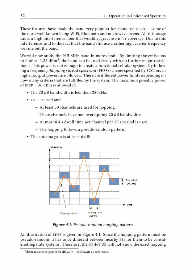
We will now study the 915 MHz band in more detail. By limiting the emissionsto eirp = -1.23 dBm3, the band can be used freely with no further major restric-tions. This power is not enough to create a functional cellular system. By follow-ing a frequency-hopping spread spectrum (fhss) scheme specified by fcc, muchhigher output powers are allowed. There are different power limits depending onhow many criteria that are fulfilled by the system. The maximum possible powerof eirp = 36 dBm is allowed if:
• The 20 dB bandwidth is less than 250kHz.
• fhss is used and
– At least 50 channels are used for hopping.
– These channels have non overlapping 20 dB bandwidths.
– At most 0.4 s dwell time per channel per 20 s period is used.
– The hopping follows a pseudo-random pattern.
• The antenna gain is at least 6 dBi.
Figure 4.1: Pseudo-random hopping pattern.
An illustration of fhss is given in Figure 4.1. Since the hopping pattern must bepseudo-random, it has to be different between nearby bss for them to be consid-ered separate systems. Therefore, the nb-iot ue will not know the exact hopping
3dBm measures power in dB with 1 milliwatt as reference.
4.3 Conclusions 33
pattern until is has decoded the cell ID, which happens in the end of the synchro-nization process when the nsss is detected. At this point, the timing is knownup to a multiple of 80 ms. Therefore, a feasible way to synchronize the ue to thebss channel hopping is to use a channel dwell time that is a multiple of 80 ms.The ue can then listen to one channel until the npss and nsss is detected andthen do hypothesis testing of the number of 80 ms periods until the next hop bysampling both the current and the next channel.
Furthermore, by having themib transmission interval of 640 ms being a multipleof the channel dwell time, the mib boundary is given by knowing the hoppingboundary, the hopping pattern and the index of the current channel. This simpli-fies mib detection. The largest channel dwell time satisfying both this criterionand the 0.4 s limit is 320 ms. The conclusion here is that nb-iot-u should be ableto finish both npss and nsss processing within 320 ms.
4.2.2 EU Short Range Devices
In the European Union, low power radiating devices are called Short Range De-vices (srd). These correspond to ism in the U.S. and include nb-iot devices. TheElectronic Communications Committee (ecc) in EU provides recommendationsfor how frequency bands should be allocated and used. The recommendationsfor srd are found in a document called Rec 70-03 [16] and are supposed so beimplemented by the member states. [14]
There is a 2.4 GHz band also for srd, which we exclude based upon previousarguments. There are also three bands around 434 MHz, which have a low powerlimit and does not allow voice. The remaining bands are listed in Table 4.1 to-gether with their relevant regulations. The 869.4 (to 869.65) MHz band is by farthe best candidate in terms of power, which is a crucial factor for nb-iot cover-age: The erp is 27 dBm corresponding to an eirp of 29.15 dBm. By concatenat-ing many channels, this band can also be operated in a mode that utilizes thefull bandwidth of 250 kHz, which matches the 915 MHz ism band nicely andallows for a similar implementation. The 10% duty cycle means that: A devicecan transmit for a maximum total time of 360 s per hour; each transmission canhave a maximum length of 36 s; a minimum off time of 3.6 s is required betweentransmissions. This should, however, be easily manageable once adaption to theism dwell time is handled.
4.3 Conclusions
The 915 MHz ism band and the 869.4 MHz srd band are the most promising forcommercial nb-iot-u deployment. What we learned from studying their regula-tions is that a number of adaptions has to be made. The changes or settings thataffect our study are the following:
1. The synchronization should not take more than 320 ms.
2. A pulse shaping filter might be needed to make sure the 20 dB bandwidth

34 4 Operation in Unlicensed Spectrum
Table 4.1: srd regulations at interesting frequencies.
Frequency Band (MHz) Channel BW erp (dBm) Duty Cycle
868.0 – 868.6 No limit 14 <1%868.7 – 869.2 No limit 14 <0.1%869.3 – 869.4 <25 kHz 10 No limit869.4 – 869.65 <25 kHz1 27 <10%869.7 – 870.0 No limit 7 No limit1 Channels may be concatenated.
lies within 250 kHz.
3. The eirp limits are 29.15 dBm and 36 dBm for EU and the U.S. respectively.
4. A carrier frequency of 900 MHz should be a good assumption in our exper-iment.
These points are incorporated into our study as described in Chapter 7.

5Temporal Diversity
This is the first chapter of two that will describe and specify the methods thatare studied in this thesis. The chapter starts with an introduction of how coher-ent combining can be used for time diversity. Then follows two sections, eachdescribing a method that is based upon coherent combining.
5.1 Coherent Combining
The synchronization accuracy is essentially limited by the snr of the received sig-nal. One way of increasing the snr is to transmit at a higher signal power. Thisis often not a feasible solution, for several reasons. Higher transmit power canincrease the detrimental effects of hardware non-linearities, it obviously leads toa higher power consumption and it might be prohibited by regulations. More-over, it may lead to higher interference within a system, which in turn actuallydegrades performance.
Another way of achieving a higher total energy of the received signal is to extendit in time. By allocating more time resources to the reference signals, more re-dundant information could be sent and enable a less uncertain estimation. Butinstead of looking at this as increased information, it could it could be treatedas an increased snr, if the signals are combined coherently. By transmitting thesame reference signal several times and then adding the copies together in the re-ceiver, the fact that the noise realizations are independent would lead to a highersnr. The power of coherently added signals scales quadratically, while the powerof added independent noise scales linearly. With N transmissions of signal s with
35

36 5 Temporal Diversity
additive white Gaussian noise, n, the resulting snr would be
snrnew =E
{|Ns|2
}E
{N |n|2
} = NE
{|s|2
}E
{|n|2
} = N · snrold (5.1)
and the snr gain would thus be 10 log10 N dB. This in an example of time diver-sity.
In the real world, estimated target values might change with time. In our case,timing offset will change due to time-drift and frequency offset will change dueto oscillator instabilities and varying Doppler shifts. Time drift is expected tobe the dominant factor. The solution to the time-variance is to apply a trackingmethod, such as a linear filter. If s is the signal, and y is the estimate, an infiniteimpulse response filter would be given by
y[n] =P∑i=0
bi s[n − i] −Q∑i=1
aiy[n − i]. (5.2)
with P and Q being design parameters. The filter coefficients would ideally becalculated using linear minimum mean squared error.
The npss processing used in this thesis applies such a filter in equation (3.6),with P = 0, Q = 1, a1 = α, b0 = 1 − α and s[n] being the auto-correlation valueAk(τ) instead of directly using the signal r. Ak(τ) could equally well be thoughtof as a signal in noise. Due to the complexity of the system model, we will setα experimentally. The rest of this chapter presents two studied methods, whichboth rely on time diversity and coherent combining.
5.2 Method 1: NPSS Densification
Recall from Chapter 3 that one out of ten subframes in every frame containsthe npss. Every npss on its own provides an opportunity for synchronizationbut since the snr can be very low, the ue will combine the npsss coherently asdescribed above. In nb-iot-u however, there is a limited time window of opportu-nity for synchronization, before the bs hops to a new carrier frequency. In orderto increase the probability of success within this time window, we will furtherincrease the npss energy by allocating even more subframes. Specifically we willintroduce a new npss per frame, and refer to this scheme as densification, orthe dense case. As Figure 5.1 shows, the original npss will be moved to a latersubframe in order to allow for uniform spacing among npss subframes withoutaffecting the broadcast channel. Uniform spacing allows for the same efficientreceiver algorithm described in Section 3.3.3, but with half the accumulation pe-riod. This would have the advantage that only half the buffer memory would beneeded in the ue receiver.
One might believe that an extra npss subframe would lead to significant over-head, occupying a potential payload subframe. This is not necessarily the case,

5.3 Method 2: NPSS Enhancement 37
baseline
dense
npss
nsss Broadcast channel
Payload or control data
Figure 5.1: New dense frame structure with an extra NPSS subframe.
however. Recall from Chapter 4 that nb-iot-u would use a frequency hoppingpattern of at least 50 hopping channels. The idea is that one or a few of thesecan be used as discovery channels. The discovery channels would be known bythe ue and contain the extra (or even all of the) synchronization signals as wellas other important system information. By synchronizing to one of these chan-nels, the ue can then communicate over all the other channels with significantlylower overhead. The natural question then becomes, why not use more than twonpss subframes? The answer is that 10 — the number of subframes in a frame— has an inconvenient prime factorization, which would complicate the synchro-nization design. And two subframes, with an increased snr of 10 log10 2 ≈ 3db, is also expected to be enough. Another reasonable prediction that could bemade about this method is that with half the accumulation period, the time-driftis smaller and thus the optimal α should be higher.
5.3 Method 2: NPSS Enhancement
If adding a full subframe may seem drastic, an alternative is to add only a fewsymbols by exploiting a property of nb-iot-u: it is standalone and therefore nolte control information is transmitted in the same band. This means that the first3 symbols in every subframe (see Figure 3.4) are available. They could be used toextend the npss, either by prepending the existing code cover, or by replacing italtogether. An important problem now arises: how should the new code cover bedesigned?
5.3.1 Design Guidelines
The ultimate goal of the code cover design is to improve the estimation and detec-tion by having the metric, ρ(τ), in equation (3.7) exhibiting a narrow mainlobeand low sidelobes. In the case of high snr, a narrow mainlobe should be a goodgoal, in order to improve estimation accuracy. In low snr however, more fo-cus should be put on the sidelobes, in order to increase detection accuracy anddecrease the far. By setting a high detection threshold and relying on the coher-ent accumulation to provide a more accurate metric ρ(τ), more focus could once
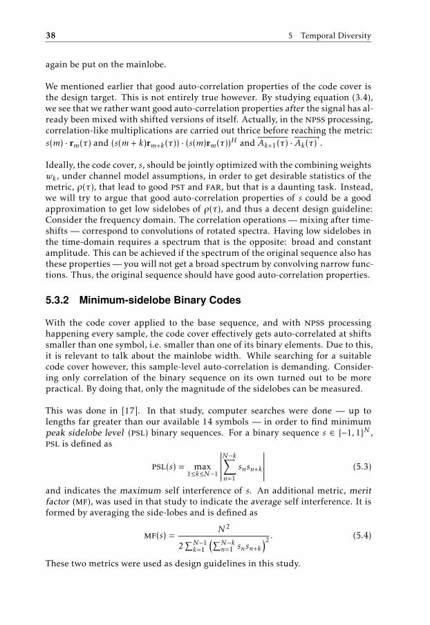
38 5 Temporal Diversity
again be put on the mainlobe.
We mentioned earlier that good auto-correlation properties of the code cover isthe design target. This is not entirely true however. By studying equation (3.4),we see that we rather want good auto-correlation properties after the signal has al-ready been mixed with shifted versions of itself. Actually, in the npss processing,correlation-like multiplications are carried out thrice before reaching the metric:s(m) · rm(τ) and (s(m + k)rm+k(τ)) · (s(m)rm(τ))H and Ak+1(τ) · Ak(τ)
∗.
Ideally, the code cover, s, should be jointly optimized with the combining weightswk , under channel model assumptions, in order to get desirable statistics of themetric, ρ(τ), that lead to good pst and far, but that is a daunting task. Instead,we will try to argue that good auto-correlation properties of s could be a goodapproximation to get low sidelobes of ρ(τ), and thus a decent design guideline:Consider the frequency domain. The correlation operations — mixing after time-shifts — correspond to convolutions of rotated spectra. Having low sidelobes inthe time-domain requires a spectrum that is the opposite: broad and constantamplitude. This can be achieved if the spectrum of the original sequence also hasthese properties — you will not get a broad spectrum by convolving narrow func-tions. Thus, the original sequence should have good auto-correlation properties.
5.3.2 Minimum-sidelobe Binary Codes
With the code cover applied to the base sequence, and with npss processinghappening every sample, the code cover effectively gets auto-correlated at shiftssmaller than one symbol, i.e. smaller than one of its binary elements. Due to this,it is relevant to talk about the mainlobe width. While searching for a suitablecode cover however, this sample-level auto-correlation is demanding. Consider-ing only correlation of the binary sequence on its own turned out to be morepractical. By doing that, only the magnitude of the sidelobes can be measured.
This was done in [17]. In that study, computer searches were done — up tolengths far greater than our available 14 symbols — in order to find minimumpeak sidelobe level (psl) binary sequences. For a binary sequence s ∈ {−1, 1}N ,psl is defined as
psl(s) = max1≤k≤N−1
∣∣∣∣∣∣∣N−k∑n=1
snsn+k
∣∣∣∣∣∣∣ (5.3)
and indicates the maximum self interference of s. An additional metric, meritfactor (mf), was used in that study to indicate the average self interference. It isformed by averaging the side-lobes and is defined as
mf(s) =N2
2∑N−1k=1
(∑N−kn=1 snsn+k
)2 . (5.4)
These two metrics were used as design guidelines in this study.
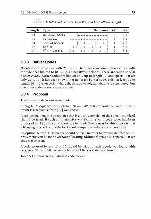
5.3 Method 2: NPSS Enhancement 39
Table 5.1: npss code covers. Low psl and high mf are sought.
Length Type Sequence psl mf
11 Baseline (3gpp) [+ + + + − − + + + − +] 2 2.914 Extension [− + + + + + + − − + + + − +] 4 1.911 Special Barker [+ + + − − − + − − + −] 1 12.113 Barker [+ + + + + − − + + − + − +] 1 14.114 Minimum psl [+ + + + + + − − + + − + − +] 2 5.2
5.3.3 Barker Codes
Barker codes are codes with psl = 1. There are also some Barker codes withthe sidelobes limited to {0, 1}, i.e. no negative sidelobes. These are called specialBarker codes. Barker codes are known only up to length 13, and special Barkeronly up to 11. It has been shown that no larger Barker codes exist, at least up tolength 1022. Barker codes where the first go-to solution that were considered, buttwo other code covers were also tried.
5.3.4 Proposal
The following decisions were made.
A length-14 sequence with optimal psl and mfmetrics should be tried: the min-imum psl sequence from [17] was chosen.
A suboptimal length-14 sequence that is a pure extension of the current standardshould be tried, if such an alternative was found: such a code cover has beenproposed in [18], and could therefore be used. The reason for this choice is thata bs using this code could be backward compatible with older version ues.
An optimal length-11 sequence should be tried in order to investigate whether im-provements can be made without allocating additional symbols: a special Barkercode was chosen.
A code cover of length 12 or 13 should be tried, if such a code was found withvery good psl and mfmetrics: a length-13 Barker code was chosen.
Table 5.1 summarizes all studied code covers.


6Spatial Diversity
In the previous chapter, we discussed methods to improve reception by makingthe reference signals more dense in time. In this chapter, we will show methodsthat might improve the overall performance of the scheme by altering the channelconditions as to mitigate the detrimental effects of fading. These methods rely onspatial diversity, using multiple transmit antennas. As we will see, a good way ofdoing this is to create artificial fast fading by blindly looping through a carefullychosen codebook.
6.1 Fading Channels in NB-IoT
Many different channel models incorporate a propagation phenomenon calledfading, which is the change in reception quality brought on by time-varying chan-nels. One important type, multipath fading, is the effect not mainly of objectsshadowing the path but of the inverse: objects in the environment cause reflec-tion and diffraction of waves, which leads to multiple incoming rays at the re-ceiver location interfering constructively or destructively. An illustration of thiseffect is given in Figure 6.1.
Due to movement of both these objects and the ue, the channel will change andthe perceived signal quality may fluctuate as the ue moves through weak andstrong spots. This is called fast fading and may or may not be a desired channelproperty in a cell. In the case of nb-iot, a great deal of ues will be stationarilydeployed1 in a static environment. If in addition to this, the fast fading is not fastenough, a particularly unfavorable situation can occur. With a Doppler spreadof less than 1 Hz for example, a substantial fraction of users would experience a
1For example the electric meter far down in your basement.
41

42 6 Spatial Diversity
deep fade (i.e. a very destructive interference) throughout the 320 ms synchro-nization window.
bs ue
g2 g1
g3
g4
Figure 6.1: Single-antenna multipath propagation
This is where diversity comes in. By having several transmit antennas, we canutilize the fact that not all of them will be at a deep fade at any give time. Eachantenna will create a unique link to the receiver, with its own channel realization,as shown in Figure 6.2. By transmitting the signal on each antenna simultane-ously and applying a unique filter to each of them, the total perceived channelcan be changed. Using N transmit antennas, the situation could also be inter-preted as a single-antenna channel with N adjustable rays. The goal is to set allthe filters so as to get a total channel response with a good quality, or at least tomitigate the effects of deep fades.
The problem during synchronization is that neither the bs nor the ue has gotany channel state information, and also that no feedback can be sent in the ul.Hence, the diversity scheme can not be adaptive to any particular ue’s situation.maximal ratio precoding and zero-forcing precoding, for example, require chan-nel state information at the transmitter and can not be used. Space-time blockcodes (e.g. the Alamouti code for two antennas) require channel state informa-tion at the receiver and can not be used. Actually, there is no way to increase theexpected snr at an arbitrary ue under these circumstances. What can be done,however, is to average out the snr over time and space by blindly altering thechannel. By regularly changing the filtering at each antenna, a faster fading willbe experienced at each ue. This could increase the chance that each ue has atleast some period of good reception during the 320 ms synchronization period.We call this technique artificial fast fading.
6.2 Motivation 43
bs ue
h1
hn
Figure 6.2: Multi-antenna multipath propagation
6.2 Motivation
In this section, the usefulness of artificial fast fading will be motivated mathemat-ically for the case of two transmit antennas. The argument can easily be extendedto larger number of antennas.
A common wireless channel model is the so called tapped delay line, where eachtap represents one propagation path — one ray — and has some attenuation andsome delay. On frequency bands smaller than the coherence bandwidth (givenby the delay spread), the effect of the delay is a phase shift of the incoming wave-form. Each ray, i, can then be represented by a complex number, gi , containinginformation about the attenuation and phase shift. The phase shift can oftenbe modelled as uniformly distributed. When there are many rays, the centrallimit theorem comes into effect, and the total channel, h =
∑i gi , can be approx-
imated by a circularly-symmetric complex normal distribution. This model iscalled Rayleigh fading.
If multiple transmit antennas are used and, additionally, the spacing betweenadjacent equally polarized antennas is larger than half the wavelength, the linkcan be treated as a vector of independent elements h = (h1, h2) ∼ CN (0, σhI).Figure 6.3 illustrates a channel realization for a two-antenna link. The sum h =h1 + h2 in the figure, will determine the gain of the channel, but h1 and h2 areindependent and unknown to the bs.
Consider the scheme in Figure 6.4. By multiplying the npss by −1 in every oddframe, we practically get total channel ha = h1 + h2 on even frames and hb = h1 −h2 on odd frames. When ha is small, hb is likely to be large, and the accumulationdone in equation (3.6) (described in Section 5.1) will average out the quality. We
44 6 Spatial Diversity
will now show that this scheme will lower the variance of the received signalpower while keeping expectancy unchanged.
The accumulation in equation (3.6) is done on the auto-correlation values Akfrom equation (3.4). The useful signal in Ak is proportional to |h|2. Thus, itmakes sense to study the sum absolute square of the channel coefficients overtwo frames when evaluating the quality of the accumulation. The expected accu-mulated signal power does not change when hb is used, as opposed to only usingha:
E
{|ha|2 + |hb |2
}= E
{|ha|2
}+E
{|hb |2
}= E
{|ha|2
}+E
{|ha|2
}= E
{|ha|2 + |ha|2
}(6.1)
The variance however, will decrease when the scheme is used:
Var{|ha|2 + |hb |2
}= Var
{|ha|2
}+ Var
{|hb |2
}+ 2 Cov
{|ha|2 , |hb |2
}=
=/i.i.d.
/= 2 Var
{|ha|2
}= 2σ4
h (6.2)
The last equality can be calculated using the fact that the square of a Rayleigh ran-dom variable is exponentially distributed. With the assumption that the channelcoherence time is significantly larger than a few frames, the variance when thescheme is not used is:
Var{|ha|2 + |ha|2
}= 4 Var
{|ha|2
}= 4σ4
h (6.3)
The takeaway from this section is that artificial fast fading will preserve the ex-pected received signal power for every user but make sure that the signal power,averaged over a few frames, stays closer to the expected value. This could lead toa situation where a larger proportion of the ues can synchronize within 320 ms.
6.3 Codebook Design
How should the extra antennas be used to take advantage of the diversity? Sincethe channel can be represented using complex coefficients, any channel realiza-tion with this representation could be reached by scaling each antenna gain withsome complex number. This corresponds to adjusting the power amplifier as wellas introducing a phase shift on each antenna. Since the receiver will perceive thetotal sum of all channels, the received signal could be written using an innerproduct, as
y = hHwx + n, h ∼ CN (0, ρhI), n ∼ CN (0, ρn) (6.4)
where the vector w ∈ CN is called the precoder vector and contains the complex
scaling factors described earlier. N is the number of transmitter antennas. wcan, within some constraints, be chosen freely at the transmitter side. A verycommon constraint to have is that of a limited transmitter power, P , translating to‖w‖22 ≤ P . The bs design we expect for deployment of nb-iot uses a single poweramplifier chain, setting all gains equal and bounding our choices by ‖w‖∞ ≤ P .In this situation, called equal gain beamforming (egb), only the phase matters:

6.3 Codebook Design 45
w ∈ TN and we get the situation illustrated in Figure 6.3.
<
=
h1
θ1
h2
θ2
Figure 6.3: By phase rotation on each antenna, the resulting channel can bevaried.
The example in Section 6.2 used two alternating precoders: wa = [1, 1]T andwb = [1,−1]T . This configuration can be written in matrix form as
W = [wa wb] =[1 11 −1
](6.5)
where each column is a precoder. We call this type of matrix a codebook andrefer to the number of columns, M, as the codebook length. For each new npsstransmission, a new precoder is used. This process repeats, once all precodershas been used. The transmission periodicity is thus equal to the codebook lengthtimes the time interval between twonpsss. Our design challenge is now to chooseW ∈ T
N×M in a way that maximizes the chance for a ue to synchronize within320 ms.
Antenna 1
Antenna 2
+npssnsss Broadcast channel
−npss
Figure 6.4: Example of subframe structure using antenna diversity.
46 6 Spatial Diversity
6.3.1 Grassmannian Line Packing
Poor channel quality is avoided by making the channel realizations as diverseas possible. This amounts to picking precoders wk that are, in some sense, farapart. The received signal power for a single transmission is proportional tohHwwHh, so in order to achieve a diverse codebook, its rows should be spreadout in a directional sense. The outer product of w is independent of phase shiftson w. Moreover, since the algorithm accumulates the timing metric instead ofthe actual signal, our performance is invariant to uniform precoder phaseshifts.
So we want to spread out w in all directions of CN as measured by inner products,i.e. to do sphere packing on the complex projective space CP
N−1. This space isequal to Gr(1,CN ), where the r-th order Grassmannian manifold, Gr(r, V ), of thevector space V , is defined as the set of r-dimensional subspaces of V . For thisreason, the problem is equivalent to Grassmannian line packing and is hencesometimes referred to as Grassmannian precoding.
Since TN is not a vector space, our problem is not directly Grassmannian line
packing, but is usually regarded as line packing on Gr(1,CN ) with egb con-straints. Grassmannian line packing on high dimensional complex space is anopen problem in mathematics. The case with one antenna is of course trivial.The two-antenna case has been solved by proving the isometric isomorphismGr(1,C2) � S2 [19]. The egb case for two antennas is trivial. For higher dimen-sions however, numerical approximations are commonly used, but can be hardto find because of the non-convexity of the optimization problem [20].
6.3.2 Hadamard Patterns
If M = N , that is if the codebook is a square matrix, the optimal Grassman-nian line packing will be achieved by any unitary matrix. For example, any or-thonormal basis in R
N is optimal, which under the egb constraint turns to bethe Hadamard matrices, if the dimension N is a power of two. Hadamard ma-trices are often defined as an example of generalized Fourier matrices, but canconveniently be defined recursively as
Hi+1 =[Hi HiHi −Hi
], H0 = [1] (6.6)
6.4 Method 3: Artificial Fast Fading
This section specifies the set of codebooks that constitute Method 3. Hadamardmatrices up to H4 will be used. Larger sizes are not expected to help much, sincethe synchronization already must be done within a handful of frames. Moreover,while the quality averaging effects for a few antennas might be useful, diminish-ing returns are expected for additional antennas. As mentioned earlier, the egbcase for N = 2 is easy. Since only the direction of w matters, the first row can bekept unchanged without loss of generality. For an M-sized code, the second rowshould contain theM-th roots of unity. We will choose the optimal Grassmannian
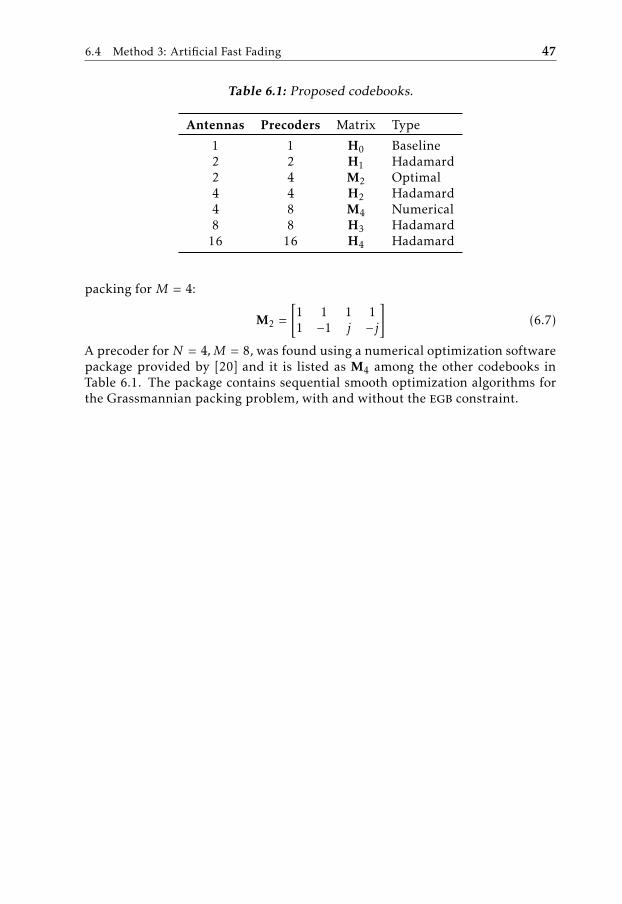
6.4 Method 3: Artificial Fast Fading 47
Table 6.1: Proposed codebooks.
Antennas Precoders Matrix Type
1 1 H0 Baseline2 2 H1 Hadamard2 4 M2 Optimal4 4 H2 Hadamard4 8 M4 Numerical8 8 H3 Hadamard
16 16 H4 Hadamard
packing for M = 4:
M2 =[1 1 1 11 −1 j −j
](6.7)
A precoder for N = 4, M = 8, was found using a numerical optimization softwarepackage provided by [20] and it is listed as M4 among the other codebooks inTable 6.1. The package contains sequential smooth optimization algorithms forthe Grassmannian packing problem, with and without the egb constraint.

7Experimental Setup
This chapter describes how the theory, background and methods introduced sofar can be used to provide answers to the questions asked in the introduction.A sequence of simulations are described whose results can be tied directly to ourmetrics. The first section outlines a step by step procedure and the second sectionspecifies the parameter settings for each simulation.
7.1 Experiment Overview
As stated in Chapter 1, we want to study the performance of different methodsfor initial cell acquisition and synchronization. Studying here refers to implemen-tation and simulation of the suggested methods under coverage conditions thatcould be considered realistic but challenging for nb-iot-u. The tool that will beused for this is a proprietary Matlab link simulator developed at Ericsson AB.
7.1.1 Objectives and Methods
As a reminder of what this study is about, we will here recapitulate our studiedmethods and research objectives. We have described three methods, two of whichhave several configurations:
• npss densification — illustrated in Figure 5.1.
• npss enhancement — with the five settings shown in Table 5.1.
• Artificial fast fading — with the seven settings shown in Table 6.1.
These methods will all be investigated by simulation as an attempt of answeringthe following questions from Section 1.3:
49

50 7 Experimental Setup
1. How can nb-iot synchronization time be decreased while keeping accuracyhigh and receiver complexity low?
2. What methods could be good candidates for nb-iot-u?
3. Would proposed candidates require a change of the current standard?
Question 1 will be approached by making a comparison of the three methods.The comparison will be relative to each other, with the main benchmark beinga low pst for almost all users. Accuracy will be controlled by using the Geniedetection rule. The complexity issue is handled by limiting the setup to use thereceiver algorithm from Section 3.3.3.
Question 2 will be answered by picking good candidate methods, set the simula-tion parameters as realistically as possible and then compare the metrics with therequirements. From Chapter 4, we learned that the time limit for full synchro-nization is 320 ms. We need 90% of users to achieve this with a far not greaterthan 5%. The far can be measured by using the Peak detection rule.
Question 3 will be answered by observing whether the answers to Question 2requires changes to the existing npss or its placement within the frame. A pureextension of the npss does not and neither does the use of method 3.
7.1.2 Experiment Procedure
The study will be carried out in a 4-step procedure. Each step will provide set-tings or other information for subsequent steps.
Step 1: Prestudy
The purpose of the prestudy is to determine how the rest of the study should beset up, in order to yield more reliable results. The first thing to do is to make surethat the bandwidth requirement stated in Section 4.3 is met by finding a suitabletransmit filter. The reason we do this is that a transmit filter may have significanteffects on performance.
The other thing that is done in the prestudy is finding a relationship betweenpst (corresponding to npss processing) and the full synchronization time (corre-sponding to both npss and nsss processing). The conclusion from Section 4.3 isthat full synchronization time should take a maximum of 320 ms. The main pur-pose of this thesis regards only pst, which is the interesting and most challengingpart of the synchronization, but nsss processing may take some non-negligibletime and must be taken into account while answering Question 2 above. Thus anew smaller time limit should be set for pst.
Step 2: Method comparison
All synchronization methods outlined in Section 7.1.1 will be simulated usingthe same baseline parameters (with the filter chosen in the Step 1) and with theonly changes being whatever is implied by the respective method.

7.2 Simulation Setup 51
These results will serve two purposes. They will be used directly to answer Ques-tion 1 by comparing the methods to the baseline and to each other. They willalso be used to select two or three candidate methods that seem promising formeeting the demands of nb-iot-u declared in Section 7.1.1 and the Step 1. Thecandidates are chosen from the methods tested in this step but may also be com-binations of these. The candidates will be studied in more detail in subsequentsteps in order to answer Question 2 and 3.
Step 3: Algorithm fine-tuning
The purpose of this step is to tune the receiver algorithm for each of the candidatemethods chosen in Step 2 so as to maximize performance. To simplify the studyand make the comparison more straightforward, Step 1 & 2 eliminate the effectsof false alarms by applying the Genie detection rule. This is not realistic anddoes not give a full picture of the performance. To answer Question 2 and 3, thecandidates are evaluated using the Peak detection rule.
There is a trade-off between pst and far. A relaxed detection threshold, λP ,leads to faster synchronization at the cost of more false alarms. The forgettingfactor, α, also affects this but its relationship is not monotonic. When α is set formaximum-ratio combining, the perceived snr is optimal, leading to a minimumfar. The relationship between α and pst is more complicated and depends alsoon λP and the snr of the individual user. In principle, a suboptimal α will leadto more false alarms which lowers the pst, but also to more false negatives1 thatincrease the pst. In Step 3, first α and then λP will be set.
Step 4: Evaluation
In the last step, the candidates are evaluated using the parameters set in Step 3.The simulations will have an increased sample size for more reliable statistics.The results will include both tables and plots showing the distributions of bothpst and residual errors. These results ought to be reliable enough to answerQuestion 2 & 3.
7.2 Simulation Setup
The system model is based upon previous studies done onnb-iot synchronizationfor standalone deployment ([3], [2], [18]) but is modified according to Section 4.3.This section summarizes the fixed system parameters as well as the baseline sim-ulation parameters and how they change for all simulation instances.
7.2.1 Basic Assumptions
The system consists of a ue receiver in a single cell with the bs transmitting overa time period of approximately 10 seconds — long enough to assure that the uewill synchronize. There are no additional cells to cause ici nor any interfering
1False negatives are often referred to as type II errors and occur when the estimate although beingaccurate is deemed too uncertain for detection.
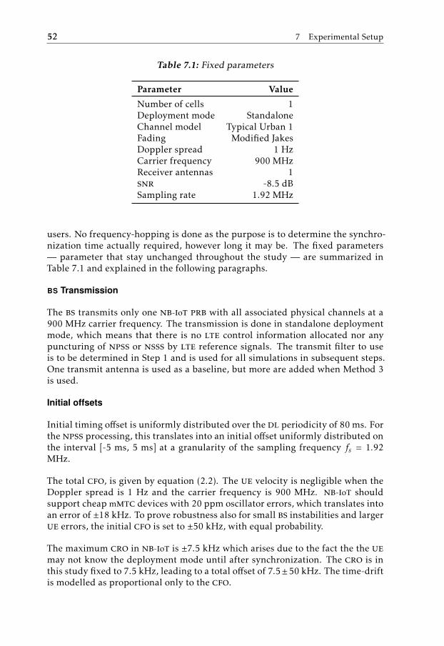
52 7 Experimental Setup
Table 7.1: Fixed parameters
Parameter Value
Number of cells 1Deployment mode StandaloneChannel model Typical Urban 1Fading Modified JakesDoppler spread 1 HzCarrier frequency 900 MHzReceiver antennas 1snr -8.5 dBSampling rate 1.92 MHz
users. No frequency-hopping is done as the purpose is to determine the synchro-nization time actually required, however long it may be. The fixed parameters— parameter that stay unchanged throughout the study — are summarized inTable 7.1 and explained in the following paragraphs.
BS Transmission
The bs transmits only one nb-iot prb with all associated physical channels at a900 MHz carrier frequency. The transmission is done in standalone deploymentmode, which means that there is no lte control information allocated nor anypuncturing of npss or nsss by lte reference signals. The transmit filter to useis to be determined in Step 1 and is used for all simulations in subsequent steps.One transmit antenna is used as a baseline, but more are added when Method 3is used.
Initial offsets
Initial timing offset is uniformly distributed over the dl periodicity of 80 ms. Forthe npss processing, this translates into an initial offset uniformly distributed onthe interval [-5 ms, 5 ms] at a granularity of the sampling frequency fs = 1.92MHz.
The total cfo, is given by equation (2.2). The ue velocity is negligible when theDoppler spread is 1 Hz and the carrier frequency is 900 MHz. nb-iot shouldsupport cheap mmtc devices with 20 ppm oscillator errors, which translates intoan error of ±18 kHz. To prove robustness also for small bs instabilities and largerue errors, the initial cfo is set to ±50 kHz, with equal probability.
The maximum cro in nb-iot is ±7.5 kHz which arises due to the fact the the uemay not know the deployment mode until after synchronization. The cro is inthis study fixed to 7.5 kHz, leading to a total offset of 7.5±50 kHz. The time-driftis modelled as proportional only to the cfo.
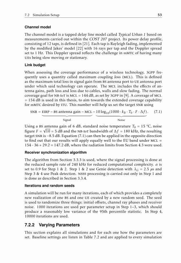
7.2 Simulation Setup 53
Channel model
The channel model is a tapped delay line model called Typical Urban 1 based onmeasurements carried out within the COST 207 project. Its power delay profile,consisting of 12 taps, is defined in [21]. Each tap is Rayleigh fading, implementedby the modified Jakes’ model [22] with 16 rays per tap and the Doppler spreadset to 1 Hz. This Doppler spread reflects the challenge in mmtc of having manyues being slow moving or stationary.
Link budget
When assessing the coverage performance of a wireless technology, 3gpp fre-quently uses a quantity called maximum coupling loss (mcl). This is definedas the maximum total loss in signal gain from bs antenna port to ue antenna portunder which said technology can operate. The mcl includes the effects of an-tenna gains, path loss and loss due to cables, walls and slow fading. The normalcoverage goal for nb-iot ismcl = 144 dB, as set by 3gpp in [9]. A coverage ofmcl= 154 dB is used in this thesis, to aim towards the extended coverage capabilityfor mmtc desired by itu. This number will help us set the target snr using
snr = eirp − bs antenna gain −mcl︸ ︷︷ ︸Signal
− 10 log10(1000 · kB · T0 · F · ∆f )︸ ︷︷ ︸Noise
. (7.1)
Using a bs antenna gain of 6 dB, standard noise temperature T0 = 15 °C, noisefigure F =
√10 = 5 dB and the nb-iot bandwidth of ∆f = 180 kHz, the resulting
target snr is −8.5 dB. Equation (7.1) can then be applied in the opposite directionto find out that our results will apply equally well to the EU band under mcl =154 - 36 + 29.2 = 147.2 dB, where the radiation limits from Section 4.3 were used.
Receiver synchronization algorithm
The algorithm from Section 3.3.3 is used, where the signal processing is done atthe reduced sample rate of 240 kHz for reduced computational complexity. α isset to 0.9 for Step 1 & 2. Step 1 & 2 use Genie detection with λG = 2.5 µs andStep 3 & 4 use Peak detection. nsss processing is carried out only in Step 1 andis done as described in Section 3.3.4.
Iterations and random seeds
A simulation will be run for many iterations, each of which provides a completelynew realization of one bs and one ue created by a new random seed. The seedis used to randomize three things: initial offsets, channel ray phases and receivernoise. 1000 iterations are used per parameter setup in Step 1–3, which shouldproduce a reasonably low variance of the 95th percentile statistic. In Step 4,10000 iterations are used.
7.2.2 Varying Parameters
This section explains all simulations and for each one how the parameters areset. Baseline settings are listen in Table 7.2 and are applied to every simulation
54 7 Experimental Setup
Table 7.2: The varying parameters, exemplified by the baseline case.
Parameter Value
npss density 1 / frameCode cover 3gppTransmit antennas 1α 0.9λG 2.5 µsλP 15Iterations 1000Transmit filter see Section 8.1
unless stated otherwise.
Prestudy
Transmit filters may be needed to limit the 20 dB bandwidth to 250 kHz. Apower spectral density estimate will be formed by generating transmit signals inthe simulator using different filters. The alternative of not using a filter at all willbe compared to the alternative of using a filter previously used in the simulatorfor studies on gsm refarming and to the alternative of designing a suitable root-raised-cosine (rrc) filter. The rrc filter will be limited to a maximum of 61 tapsand designed for a flat passband response while meeting the leakage limit. Worthmentioning is that an rrc filter is used at the receiver.
Using the results from the filter selection, an affine relationship will be foundbetween pst and full synchronization time by linear regression. The model as-sumed here is that the nsss processing time consists of a constant mean inde-pendent of the npss processing time plus a dependent part proportional to npss.The pst corresponding to a full synchronization time of 320 ms will be used asour target.
Comparison
Method 1 will be tested by running the baseline (with npss in subframe 6) and byrunning the dense case (with npss in subframes 2 & 7). The forgetting factor willbe kept unchanged although the dense case is expected to favor a higher value ofthe parameter. The chance for adjustment comes in Step 3.
Method 2 will be tested similarly, with the baseline compared to all code covers.
Method 3 will be tested with different numbers of antennas that all transmit thesame signal, changed only by the precoder. The power is spread evenly betweenantennas and normalized to sum up to the same transmit power used in the base-line. One precoder corresponds to a column in the codebook matrix and is mul-tiplied element wise to the antennas. Each new npss transmission will changeprecoder to the next one in the matrix, e.g. such that a 2 × 4 codebook has aperiod time of 4 frames.

7.2 Simulation Setup 55
Algorithm fine-tuning
The candidates selected in Step 2 correspond to a specific setting of one method,such as a specific code cover or codebook. Based on the parameters from Step 2,each candidate are run in Peak detection mode with a number of settings for α.Next, the best α is used for simulations with a number of settings for λP .
The choice of these parameters amount to a the trade-off between pst and farand thus far needs to be defined, i.e. in terms of maximum acceptable residualerrors. One part of the prestudy not yet mentioned in this report is a comparisonof residual frequency and timing errors. As it turned out from that study, thetiming estimation is by large the most challenging part. Given an accurate timing,the subsequent frequency error was well within the 50 Hz requirement definedin [9]. We thus define far based on a timing error of 5 µs, to cover up for the lowsample rate of 240 kHz used for npss processing. The 3gpp requirements are 2.5µs but are on the other hand set very tightly and may indeed be relaxed. [9]
Evaluation
10000 iterations are used in Step 4. Moreover, the best α and λP from Step 3 areused. The rest is unchanged from Step 2.

8Results
This chapter presents the results of all steps described in the previous chapter.Most experiments measure how pst is distributed for a particular parametersetup. The ecdf plots generated using this data look similar to exponential dis-tributions, and are rather smooth. For this reason, these plots are in most placesreplaced by ecdf tables, which facilitate assessment of performance. The studyis carried out in several steps (as outlined in Section 7.1.2) and each top-levelsection in this chapter corresponds to one such step. Decisions made based uponthe results of one step are motivated in the corresponding section.
8.1 Prestudy
In addition to the following, some less interesting prestudies were done. Theseinclude replication of previous studies ([3], [2], [18]) and coarse tuning of thereceiver algorithm.
8.1.1 Pulse Shaping
An rrc filter was designed with two criteria in mind: meeting the 20 dB band-width of 250 kHz and keeping the frequency response flat within the 180 kHzprb. Three parameters were used for this: roll-off factor (β), oversampling factor(OS) and filter length (truncation). Another filter that was found in the preex-isting simulator was also considered. That filter had been used for studies on li-censed standalone deployments for nb-iot and was designed to fit the gsm-mask.
The transmit signal was passed through these filters and power spectral densitiesof the outputs were estimated. The one-sided Welch estimates are shown in Fig-ure 8.1. The gsm filter meets the 20 dB bandwidth but is showing decline at the
57

58 8 Results
50 100 150 200 250 300−50
−45
−40
−35
−30
−25
−20
−15
−10
−5
0
Frequency [kHz]
Pow
er/F
requ
ency
[dB
/Hz]
57-tap rrc, β=0.3, OS=819-tap gsmmaskNo filter
Figure 8.1: Welch PSD estimate of the transmit signal, showing the 20 dBbandwidths for different transmit filters.
Table 8.1: pst [ms] for different transmit filters
ecdf No filter gsmmask rrc
50% 50 50 4090% 270 280 26095% 430 420 34099% 820 810 770
edge of the prb. The rrc filter on the other hand meets the 20 dB bandwidthwith an even larger marginal while keeping the in-band response similar to theunfiltered signal. Table 8.1 shows that the performance of the gsm filter is no-ticeably but not overwhelmingly worse than that of the rrc filter. The rrc filter,having a length of 57 taps, unfortunately suffered from prohibitively long simula-tion times — an effect that might arise also in bs implementations. The gsm filterwas chosen for our study and more rigorous filter designs could be considered forfuture studies.
8.1.2 Target Latency
Performing a large number ofnsss processing simulations was out of the scope ofthis study. One simulation using the baseline setup was done however, with someresults plotted in Figure 8.2 together with a linear fit. The regression line can be

8.2 Method Comparison and Selection 59
interpreted as showing the (sample) average time required for nsss processing,given that the npss processing took a certain time. The linear model is motivatedby the assumption that thensss processing relies on low residualnpss processingerrors, which given a robust detection rule should be largely uncorrelated to thesnr, leading to the constant term. The scaling factor is due to the fact that nsssprocessing still relies on good reception of the nsss, which depend on the snr.
y = 320 ms gives us x = 259.4 ms (see linear fit in Figure 8.2), which means thatwhennpss takes (i.e. pst is) 259.4 ms, the full synchronization is expected to take320 ms. Our objective is to maximize the worst case performance as opposed tothe average case. On the other hand, the nsss processing used in the simulationsare off-the-shelf and perhaps far from optimal. 260 ms is chosen as the 90thpercentile pst target, with the repercussions of this compromise addressed inChapter 9.
500 1,000 1,500 2,000
500
1,000
1,500
2,000
npss synchronization time [ms]
npss
+nsss
sync
hron
izat
ion
tim
e[m
s]
DataLinear fit: y = 1.029x + 52.83
Figure 8.2: Relationship of synchronization time between primary and sec-ondary synchronization.
8.2 Method Comparison and Selection
This section corresponds to Step 2. Each of the three methods are tested using1000 iterations and the gsm filter.
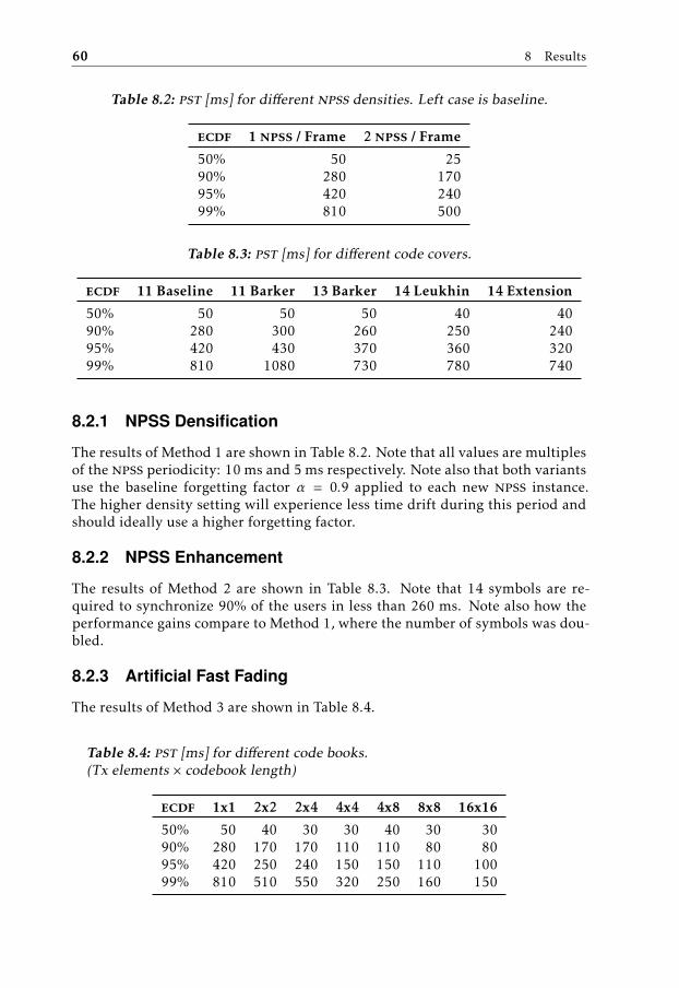
60 8 Results
Table 8.2: pst [ms] for different npss densities. Left case is baseline.
ecdf 1 npss / Frame 2 npss / Frame
50% 50 2590% 280 17095% 420 24099% 810 500
Table 8.3: pst [ms] for different code covers.
ecdf 11 Baseline 11 Barker 13 Barker 14 Leukhin 14 Extension
50% 50 50 50 40 4090% 280 300 260 250 24095% 420 430 370 360 32099% 810 1080 730 780 740
8.2.1 NPSS Densification
The results of Method 1 are shown in Table 8.2. Note that all values are multiplesof the npss periodicity: 10 ms and 5 ms respectively. Note also that both variantsuse the baseline forgetting factor α = 0.9 applied to each new npss instance.The higher density setting will experience less time drift during this period andshould ideally use a higher forgetting factor.
8.2.2 NPSS Enhancement
The results of Method 2 are shown in Table 8.3. Note that 14 symbols are re-quired to synchronize 90% of the users in less than 260 ms. Note also how theperformance gains compare to Method 1, where the number of symbols was dou-bled.
8.2.3 Artificial Fast Fading
The results of Method 3 are shown in Table 8.4.
Table 8.4: pst [ms] for different code books.(Tx elements × codebook length)
ecdf 1x1 2x2 2x4 4x4 4x8 8x8 16x16
50% 50 40 30 30 40 30 3090% 280 170 170 110 110 80 8095% 420 250 240 150 150 110 10099% 810 510 550 320 250 160 150

8.3 Algorithm Fine-tuning 61
Table 8.5: pst [ms] and far for different forgetting factors.Candidate 1: 4x4 codebook, 1 npss per frame
ecdf α = 0.90 0.93 0.95 0.96 0.97
50% 60 70 70 80 9090% 220 220 220 230 25095% 310 300 300 310 32099% 520 480 480 480 490
far 8.2% 7.7% 6.9% 6.2% 5.7%
8.2.4 Candidate Selection
By comparing all previous results to our target of 90%, it seems that denser npssalone, or alternatively 2 transmit antennas alone, would be more than enough tomeet our goals. Further investigation showed that this is not the case. The rea-son is that the previous simulations studied estimation performance, using Geniedetection. When applying Peak detection, false alarms are introduced, which inturn forces the use of very strict detection thresholds that lead to longer synchro-nization times.
After a quick investigation, the following 2 candidate methods were chosen:
• 1 npss per frame with 4 transmit antennas.
• 2 npss per frame with 2 transmit antennas.
The choice of codebook seemed rather arbitrary based on the results, so theHadamard codebooks were chosen. To limit the scope of the study, Method 2(with its relatively low performance gains) was not studied further.
8.3 Algorithm Fine-tuning
For the 2 chosen candidate methods, the next step is to first choose α and thenλP . α is chosen for minimal 90th percentile pst. λP is chosen for the trade-offbetween a 260 ms 90th percentile pst and a 5% far.
8.3.1 Candidate 1
Candidate 1 uses 1 npss per frame and 4 transmit antennas with the H2 code-book.
Forgetting factor
The results in Table 8.5 show that the best worst-case pst performance was achievedfor α = 0.93 and α = 0.95. The average, α = 0.94, was chosen as a compromise.

62 8 Results
Table 8.6: pst [ms] and far for different detection thresholds.Candidate 1: 4x4 codebook, 1 npss per frame, α = 0.94
ecdf λP = 15 16 17 18 19 20
50% 70 70 80 80 90 9090% 220 240 250 270 280 30095% 300 320 340 360 400 43099% 480 520 590 600 710 760
far 7.1% 6.4% 5.7% 4.9% 4.5% 4.3%
Table 8.7: pst [ms] and far for different forgetting factors.Candidate 2: 2x2 codebook, 2 npss per frame
ecdf α = 0.90 0.93 0.95 0.96 0.97
50% 40 40 45 45 5090% 255 240 225 220 23095% 380 355 325 310 33099% 875 665 655 595 575
far 7.8% 7.7% 7.2% 5.9% 5.1%
Threshold
The results in Table 8.6 show that λP = 17 yields a 90% pst below 260 ms, but afar greater than 5%. λP = 18 was chosen, since the far is just below 5%. Notethat the pst ecdf values are given as multiples of 10 ms frames and that thepercentile values are rounded upwards. The exact ecdf value for 260 ms mightbe close to 90% and will be illustrated in the evaluation Step.
8.3.2 Candidate 2
Candidate 2 uses 2 npsss per frame and 2 transmit antennas with the H1 code-book.
Forgetting factor
The results in Table 8.7 show that the best worst-case pst performance is achievedfor α = 0.96, which was chosen.
Threshold
The results in Table 8.8 show that only λP = 17 satisfies both the pst and farrequirements. This value was chosen for evaluation.
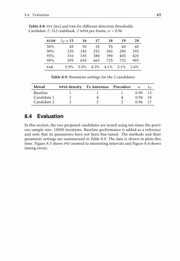
8.4 Evaluation 63
Table 8.8: pst [ms] and far for different detection thresholds.Candidate 2: 2x2 codebook, 2 npss per frame, α = 0.96
ecdf λP = 15 16 17 18 19 20
50% 45 50 55 55 60 6090% 220 245 255 265 280 29595% 310 335 380 390 405 42099% 595 655 665 725 725 905
far 5.9% 5.5% 4.3% 4.1% 3.1% 2.6%
Table 8.9: Parameter settings for the 2 candidates
Metod npss density Tx Antennas Precoders α λPBaseline 1 1 1 0.90 15Candidate 1 1 4 4 0.94 18Candidate 2 2 2 2 0.96 17
8.4 Evaluation
In this section, the two proposed candidates are tested using ten times the previ-ous sample size: 10000 iterations. Baseline performance is added as a referenceand note that its parameters have not been fine-tuned. The methods and theirparameter settings are summarized in Table 8.9. The data is shown in plots thistime. Figure 8.3 shows pst zoomed to interesting intervals and Figure 8.4 showstiming errors.
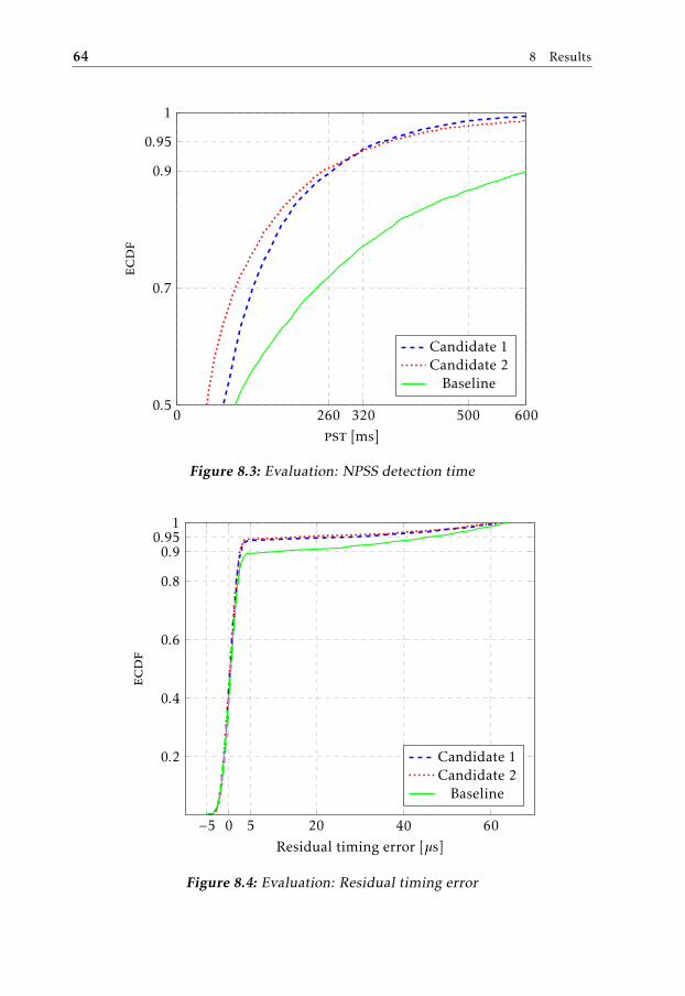
64 8 Results
0 260 320 500 6000.5
0.7
0.9
0.95
1
pst [ms]
ecdf
Candidate 1Candidate 2
Baseline
Figure 8.3: Evaluation: NPSS detection time
−5 0 5 20 40 60
0.2
0.4
0.6
0.8
0.90.95
1
Residual timing error [µs]
ecdf
Candidate 1Candidate 2
Baseline
Figure 8.4: Evaluation: Residual timing error
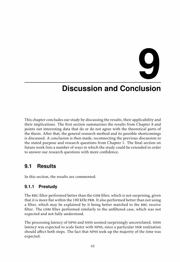
9Discussion and Conclusion
This chapter concludes our study by discussing the results, their applicability andtheir implications. The first section summarizes the results from Chapter 8 andpoints out interesting data that do or do not agree with the theoretical parts ofthe thesis. After that, the general research method and its possible shortcomingsis discussed. A conclusion is then made, reconnecting the previous discussion tothe stated purpose and research questions from Chapter 1. The final section onfuture work lists a number of ways in which the study could be extended in orderto answer our research questions with more confidence.
9.1 Results
In this section, the results are commented.
9.1.1 Prestudy
The rrc filter performed better than the gsm filter, which is not surprising, giventhat it is more flat within the 180 kHz prb. It also performed better than not usinga filter, which may be explained by it being better matched to the rrc receivefilter. The gsm filter performed similarly to the unfiltered case, which was notexpected and not fully understood.
The processing latency of npss and nsss seemed surprisingly uncorrelated. nssslatency was expected to scale faster with npss, since a particular snr realizationshould affect both steps. The fact that npss took up the majority of the time wasexpected.
65
66 9 Discussion and Conclusion
9.1.2 Method Selection
Extension of the code cover showed slight improvement, but of course not asgood improvement as the npss densification, which in principle corresponds toadding 11 symbols to the code cover.
The fact that the Barker codes did not come out superior was a bit interesting,given the argument that good auto-correlation properties should suit the syn-chronization scheme. The fact that the extended baseline sequence performedwell was welcomed, for it is the only alternative that can provide backward com-patibility.
Transmit antenna diversity was showed to yield a good improvement but only upto eight antennas. This is thought to have two main reasons. For the first 80 ms,only eight precoding patterns can be used, and by using eight antennas, thesepatterns will be orthogonal and thus optimal. Additional antennas can only behelpful if the synchronization takes more than 80 ms. Secondly, by using eightantennas, the channel quality will already be averaged out significantly, with di-minishing returns on each additional antenna. Note also that increasing only thenumber of antennas is much more effective than increasing only the codebooklength. The effect of having a number of precoders larger than the number ofantennas was not explored theoretically in the thesis and had to be tested exper-imentally. The idea behind using this was that successful synchronization couldperhaps be achieved by making sure at least one channel realization is very good,as opposed to relying on accumulation and the average channel quality.
9.1.3 Algorithm Fine-Tuning
The two chosen values for α did not differ a lot, considering the limited gainsthat can be made by very high values for α during the relatively short time frameneeded for npss processing. No prediction was made regarding which candidateshould end up with the highest α. Candidate 1 with many antennas should fa-vor a high value, to effectively utilize the different realizations. But Candidate2 should also favor a high value, since the time drift between two consecutivenpss transmissions is smaller. Both candidates has values higher than the inter-val [0.5, 0.9] suggested by [2].
No particular observations were done regarding the detection threshold.
9.1.4 Evaluation
Both methods performed significantly better than the baseline in both pst andfar at the same time. This should be expected, given the results from the methodselection. Candidate 1 barely miss the target of a 90th percentile pst of 260 mswhile Candidate 2 barely achieve it. Note also from Figure 8.3 that in terms ofpst, Candidate 1 favors worst-case users more compared to Candidate 2, whichfavors average users more. The residual errors that lie within [-2 µs, 2 µs] seem tobe uniformly distributed. These could be explained as quantization errors causedby the lower npss processing sampling rate of 240 kHz.

9.2 The Work in a Wider Perspective 67
Both candidates perform similarly in terms of far and barely miss the target of 5µs for 5% of the users. Improvement of the far turned out to be very challenging,which stems from a peculiar effect visible in Figure 8.4: while most of the timingerrors were confined to 5 µs, some errors were as large as 65 µs, corresponding toone ofdm symbol. And these larger errors were only visible for positive values.
The explanation for this comes down to how the receiver algorithms fundamen-tally works. For all code covers, the timing metric has a sharp peak centeredat zero, but with rather high and asymmetric side lobes within the symbol time,even when no channel or noise is added. Figure 2.5 illustrates this effect. Thedata is taken from the prestudy and shows the value of L1 = ρ after 30 accumula-tions. When lower values of λP was used, essential false alarms occurred: thoseerrors appeared to be uniformly distributed over the whole frame of [-5 ms, 5ms], which one should expect from false alarms.
9.2 The Work in a Wider Perspective
The purpose of this thesis was twofold: to increase performance for nb-iot andto enable nb-iot-u. Better performance of nb-iot might lead to a faster or morewidespread adoption of mmtc devices, which in turn could be a step in the di-rection towards The Networked Society. The Networked Society is a vision of atime when all things that could benefit from connectivity will be connected. Thesocietal impacts of such a situation are hard to predict but will undoubtedly bevast — far beyond the scope of this discussion.
The adaption of nb-iot for unlicensed spectrum could have many effects, someof which are discussed in Section 4.1. For example, it could lead to an overallmore efficient use of the limited amount of available radio spectrum. It couldopen up for small operators or businesses to set up wireless networks, small orlarge. It could also increase the prevailing interference in these bands, potentiallyobstructing some of the current usages.
9.3 Conclusions
The purpose of this thesis was to aid the design of nb-iot-u by studying the per-formance of various methods for initial cell acquisition and synchronization innb-iot. This goal could be considered fulfilled, since the results could be usedto make decisions on either further research or on system design. In the follow-ing section, the specific research questions stated in the problem formulation areaddressed.
9.3.1 Answers to the Research Questions
How can nb-iot synchronization time be decreased while keeping accuracy highand receiver complexity low?
It can be decreased significantly either by introducing an extra npss per frame,

68 9 Discussion and Conclusion
or by using artificial fast fading with two, four or eight antennas. An extensionof the current npss to cover a whole subframe would decrease synchronizationtime slightly.
What methods could be good candidates for nb-iot-u?
It has been shown with two candidate methods that for users with a coupling lossas weak as 154 dB, 90% will detect npss within 260 ms with only 5% having aresidual timing error greater than 5 µs. One of the methods uses four antennas,while the other uses only two antennas but an additional npss per frame. Giventhat nsss processing could benefit from similar methods, and that mcls lowerthan 154 dB are acceptable, these methods should suffice to handle the synchro-nization for successful nb-iot-u operation.
Would those candidates require a change of the current standard?
The use of bs transmit diversity would not require any change to the currentstandard since, by using the studied receiver algorithm, the ue is agnostic to theadditional antennas. npss densification would definitely require a change to thestandard and not be backward compatible since the broadcast channel hinders auniform spacing of two npsss within a frame without moving the prevalent npss.Extending the npss by appending three new symbols would require the standardto be changed, but the sequence would be backward compatible with old ues.
9.3.2 Implications
Operation of nb-iot in unlicensed spectrum was approved as a work item in theMulteFire organization in June 2017. This means that the organization will initi-ate efforts to research and standardize the corresponding technology. Cell acqui-sition and synchronization is one of the more challenging parts of this process.This thesis provides insight for that development.
9.4 Future Work
This section describes some ways in which this study could be extended to pro-vide more reliable information in the synchronization design.
The full synchronization procedure, consisting ofnpss andnsss processing, shouldbe measured. While doing this, improvements to the nsss processing should beexplored and taken into account.
Interference could be added into the model to more accurately reflect the environ-ment in unlicensed spectrum. Interference could easily and perhaps accuratelybe modeled as an additional source of white noise. Separate studies should becarried out to motivate this and to determine appropriate interference levels.
Proper design of transmit filters could be done to potentially show improvedresults.

9.4 Future Work 69
The optimal code cover should be used. It could be found by joint optimizationof code cover with the combining weights, wk . Knowing exactly how this shouldbe carried out require some more thorough theoretical analysis of the estimationbounds and how they relate to high percentile psts. Of course, it could still beworthwhile to explore totally different synchronization algorithms.
Antenna code books could be studied further. First of all it should be clarifiedwhether increased code book sizes provide any useful gain. Then code book sort-ing could be studied to make sure the precoders are deployed in the correct order(applicable only to the case of large code books). Finally, studies on the effect ofrelaxing the egb requirements should be done.
Totally different methods for transmit diversity could also be studied. Differen-tial space-time codes is an example of a group of transmit diversity schemes thatdoes not require channel knowledge in the transmitter nor in the receiver. Theapplicability of such schemes in the synchronization phase could be interestingto explore.


List of Figures
2.1 Block model of a communication link . . . . . . . . . . . . . . . . . 72.2 Frame structure using: a) optimal codec b) modular design . . . . 82.3 OFDM demodulator with local oscillator (fc) and sample clock (fs)
separated. [Source: Wikimedia Commons (remix)] . . . . . . . . . 92.4 Timing offset, CFO and CRO. The scaling of the axes preserves
area and will for high carrier frequencies be perceived as anotherconstant offset. . . . . . . . . . . . . . . . . . . . . . . . . . . . . . . 11
2.5 Example of a timing metric. The data is taken from the prestudyand the cost function is |ρ| (defined in the next chapter). . . . . . . 14
3.1 The importance of key capabilities in different usage scenarios. [Source:IMT Vision, ITU] . . . . . . . . . . . . . . . . . . . . . . . . . . . . . 20
3.2 NB-IoT deployment modes. [Source: Ericsson Research Blog] . . . 213.3 NB-IoT frame structure . . . . . . . . . . . . . . . . . . . . . . . . . 223.4 NPSS resource mapping, inband deployment. Each row represents
one subcarrier. . . . . . . . . . . . . . . . . . . . . . . . . . . . . . . 233.5 NB-IoT NPSS structure, standalone deployment. . . . . . . . . . . 25
4.1 Pseudo-random hopping pattern. . . . . . . . . . . . . . . . . . . . 32
5.1 New dense frame structure with an extra NPSS subframe. . . . . . 37
6.1 Single-antenna multipath propagation . . . . . . . . . . . . . . . . 426.2 Multi-antenna multipath propagation . . . . . . . . . . . . . . . . 436.3 By phase rotation on each antenna, the resulting channel can be
varied. . . . . . . . . . . . . . . . . . . . . . . . . . . . . . . . . . . . 456.4 Example of subframe structure using antenna diversity. . . . . . . 45
8.1 Welch PSD estimate of the transmit signal, showing the 20 dBbandwidths for different transmit filters. . . . . . . . . . . . . . . . 58
8.2 Relationship of synchronization time between primary and secondarysynchronization. . . . . . . . . . . . . . . . . . . . . . . . . . . . . . 59
8.3 Evaluation: NPSS detection time . . . . . . . . . . . . . . . . . . . . 648.4 Evaluation: Residual timing error . . . . . . . . . . . . . . . . . . . 64
71
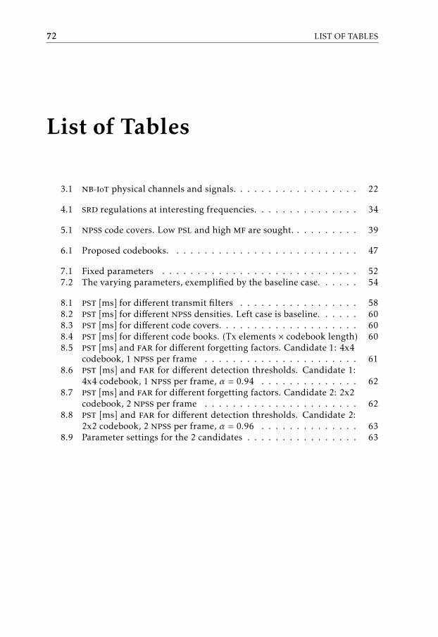
72 LIST OF TABLES
List of Tables
3.1 nb-iot physical channels and signals. . . . . . . . . . . . . . . . . . 22
4.1 srd regulations at interesting frequencies. . . . . . . . . . . . . . . 34
5.1 npss code covers. Low psl and high mf are sought. . . . . . . . . . 39
6.1 Proposed codebooks. . . . . . . . . . . . . . . . . . . . . . . . . . . 47
7.1 Fixed parameters . . . . . . . . . . . . . . . . . . . . . . . . . . . . 527.2 The varying parameters, exemplified by the baseline case. . . . . . 54
8.1 pst [ms] for different transmit filters . . . . . . . . . . . . . . . . . 588.2 pst [ms] for different npss densities. Left case is baseline. . . . . . 608.3 pst [ms] for different code covers. . . . . . . . . . . . . . . . . . . . 608.4 pst [ms] for different code books. (Tx elements × codebook length) 608.5 pst [ms] and far for different forgetting factors. Candidate 1: 4x4
codebook, 1 npss per frame . . . . . . . . . . . . . . . . . . . . . . 618.6 pst [ms] and far for different detection thresholds. Candidate 1:
4x4 codebook, 1 npss per frame, α = 0.94 . . . . . . . . . . . . . . 628.7 pst [ms] and far for different forgetting factors. Candidate 2: 2x2
codebook, 2 npss per frame . . . . . . . . . . . . . . . . . . . . . . 628.8 pst [ms] and far for different detection thresholds. Candidate 2:
2x2 codebook, 2 npss per frame, α = 0.96 . . . . . . . . . . . . . . 638.9 Parameter settings for the 2 candidates . . . . . . . . . . . . . . . . 63
Bibliography
[1] ITU-R, IMT Vision Framework and Overall Objectives of the Future Devel-opment of IMT for 2020 and Beyond, September 2015. RecommendationM.2083-0. Cited on pages 1 and 19.
[2] Q. Incorporated, “NB-PSS and NB-SSS Design (Revised),” TS R1-161981,3rd Generation Partnership Project (3GPP), Mar. 2016. Cited on pages 2, 24,25, 51, 57, and 66.
[3] A. Adhikary, X. Lin, and Y.-P. E. Wang, “Performance evaluation of NB-IoTcoverage.” Submitted to IEEE Veh. Technol. Conf. (VTC), September 2016.Cited on pages 2, 51, and 57.
[4] M. Morelli, C. C. J. Kuo, and M. O. Pun, “Synchronization techniques fororthogonal frequency division multiple access (OFDMA): A tutorial review,”Proceedings of the IEEE, vol. 95, pp. 1394–1427, July 2007. Cited on pages12, 15, and 16.
[5] T. M. Schmidl and D. C. Cox, “Robust frequency and timing synchronizationfor OFDM,” IEEE Transactions on Communications, vol. 45, pp. 1613–1621,December 1997. Cited on pages 15 and 16.
[6] K. Shi and E. Serpedin, “Coarse frame and carrier synchronization of OFDMsystems: A new metric and comparison,” IEEE Transactions on WirelessCommunications, vol. 3, pp. 1271–1284, July 2004. Cited on pages 16and 25.
[7] M. Morelli and U. Mengali, “An improved frequency offset estimator forOFDM applications,” IEEE Communications Letters, vol. 3, pp. 75–77,March 1999. Cited on pages 16 and 25.
[8] Y.-P. E. Wang, X. Lin, A. Adhikary, A. Grövlen, Y. Sui, Y. W. Blankenship,J. Bergman, and H. S. Razaghi, “A primer on 3GPP narrowband internetof things (NB-IoT),” CoRR, vol. abs/1606.04171, 2016. Cited on pages 20and 27.
[9] 3GPP, “Cellular system support for ultra-low complexity and low through-
73
74 Bibliography
put Internet of Things (CIoT),” TS 45.820-d10, 3rd Generation PartnershipProject (3GPP), Nov. 2015. Cited on pages 20, 53, and 55.
[10] 3GPP, “Evolved Universal Terrestrial Radio Access (E-UTRA); Physicalchannels and modulation,” TS 36.211, 3rd Generation Partnership Project(3GPP), Jan. 2017. Cited on page 21.
[11] B. Popovic, “Generalized chirp-like polyphase sequences with optimumcorrelation properties,” IEEE Transactions on Information Theory, vol. 38,pp. 1406–1409, July 1992. Cited on page 24.
[12] Q. Incorporated, “NB-PSS and NB-SSS Design,” TS R1-161936, 3rd Genera-tion Partnership Project (3GPP), Mar. 2016. Cited on page 25.
[13] E. Dahlman, S. Parkvall, and J. Sköld, 4G, LTE-Advanced Pro and The Roadto 5G. London: Elsevier Science, 2016. Cited on page 30.
[14] M. Loy, R. Karingattil, and L. Williams, “ISM-Band and Short Range DeviceRegulatory Compliance Overview,” TS SWRA048, Texas Instruments, May2005. Cited on pages 31 and 33.
[15] FCC, “Code of Federal Regulations, Title 47, Part 15,” TS 47 CFR 15, FederalCommunications Commission (FCC), Feb. 2017. Cited on page 31.
[16] ECC, “ERC Recommendation 70–03,” TS 70–03, European Conference ofPostal and Telecommunications Administrations (CEPT), Feb. 2017. Citedon page 33.
[17] A. Leukhin and E. Potehin, “Binary sequences with minimum peak sidelobelevel up to length 68,” ArXiv e-prints, Dec. 2012. Cited on pages 38 and 39.
[18] Huawei, HiSilicon, Neul, “On cell search and system acquisition time im-provements,” TS R1-1707027, 3rd Generation Partnership Project (3GPP),May 2017. Cited on pages 39, 51, and 57.
[19] R.-A. Pitavaland, H.-L. Määttänen, K. Schober, O. Tirkkonen, and R. Wich-man, “Beamforming codebooks for two transmit antenna systems based onoptimum grassmannian packings,” IEEE Transactions on Information The-ory, vol. 57, pp. 6591 – 6602, Oct 2011. Cited on page 46.
[20] A. Medra and T.-N. Davidson, “Flexible codebook design for limited feed-back systems via sequential smooth optimization on the grassmannian man-ifold,” IEEE Transactions on Signal Processing, vol. 62, pp. 1305 – 1318, Jan2014. Cited on pages 46 and 47.
[21] 3GPP, “Radio transmission and reception,” TS GSM 05.05, 3rd GenerationPartnership Project (3GPP), Mar. 1996. Cited on page 53.
[22] P. Dent, G. Bottomley, and T. Croft, “Jakes’ fading model revisited,” IEEEElectronic Letters, vol. 29, pp. 1162–1163, June 1993. Cited on page 53.