PERFORMANCE MEASUREMENT AND

MATHEMATICAL MODELLING OF INTEGRATED

SOLAR WATER HEATERS

CELINE GARNIER

BEng in Energy and Environmental

A thesis submitted in partial fulfilment of the requirements of Edinburgh

Napier University for the award of Doctor of Philosophy.

March 2009

ABSTRACT

In a period of rapidly growing deployment of sustainable energy sources the exploitation of solar energy systems is imperative. Colder climates like those experienced in Scotland show a good potential in addressing the thermal energy requirement of buildings; particularly for hot water derived from solar energy. The result of many years of global research on solar water heating systems has outlined the promising approach of integrated collector storage solar water heaters (ICS-SWH) in cold climates. This calls for a need to estimate the potential of ICS-SWH for the Scottish climate.

This research project aims to study and analyse the performance of a newly developed ICS-SWH for Scottish weather conditions, optimise its performance, model its laboratory and field performance together with its environmental impacts and analyse its integration into buildings and benefits of such a heating system, for the primary purpose of proposing a feasible ICS-SWH prototype. Laboratory and field experiments were performed to investigate the performance of the newly developed ICS-SWH and the parameters affecting it which were fundamental to modelling its performance. This was followed by developing a thermal macro-model able to compare the temperature variation in different ICS-SWH designs; including internal temperature and external weather conditions for a given aspect ratio and to evaluate the performance of this ICS-SWH for laboratory and field conditions. This was followed by a three-dimensional Computational Fluid Dynamic (CFD) analysis of the ICS-SWH in order to optimise the fin spacing as a means of improving its performance. A Life Cycle Assessment (LCA) and monetary analysis considering the whole life energy of the different ICS-SWH designs were carried out using a previously developed thermal model in order to establish the most viable ICS-SWH with the smallest carbon footprint. Finally, a study to show how the ICS-SWH could be integrated into buildings and its potential benefits to builders and households was undertaken.

Through this work, important parameters for modelling laboratory and field performance of ICS-SWH are established. The innovative modelling tool developed can predict the bulk water temperature of the ICS-SWH for any orientation and location in the world with good accuracy. Improvements of the ICS-SWH fin design were suggested through the CFD analysis while keeping the costs to a minimum. The ICS-SWH prototype showed a high commercial potential due to its environmental and monetary benefits as well as its potential for integration into commonly used solar water heating installations and modern methods of construction such as roof panels which could result in a viable commercialisation of the prototype.

i

ACKNOWLEDGEMENTS

I would like to take the opportunity to thank my supervisors Mr John Currie and

Prof Tariq Muneer for their support and guidance throughout the course of my research.

Furthermore, I am grateful for the assistance I have received from the technician Mr Ian

Campbell and his practical know-how. Further, I would like to give my appreciation to

the PhD student Haroon Junaidi and my friend Alexander Scott-Tonge for providing

advice and support throughout my research. My coach and friend Alexandra Stellatou

was supporting me everyday of my present tenure for which I am sincerely grateful.

Finally, this research would not have happened without the love and support of my

friends and family.

C’est dans l’effort que l’on trouve la satisfaction et non dans la réussite. Un plein effort

est une pleine victoire.

The pleasure lies in making the effort, not in its fulfilment.

Gandhi, Extrait des Lettres à l'Ashram

ii

DECLARATION

I hereby declare that the work presented in this thesis was solely carried out by myself

at Edinburgh Napier University, except where due acknowledgement is made, and that

is has not been submitted for any other degree.

……………………………………………

CELINE GARNIER (CANDIDATE)

…………………..

Date

iii

TABLE OF CONTENTS

ABSTRACT……..............................................................................................................i

ACKNOWLEDGEMENTS............................................................................................ii

DECLARATION............................................................................................................iii

TABLE OF CONTENTS...............................................................................................iv

LIST OF FIGURES........................................................................................................ix

LIST OF TABLES........................................................................................................xiv

NOMEMCLATURE.....................................................................................................xv

CHAPTER 1 INTRODUCTION...............................................................................1

1.1 Energy................................................................................................................1

1.1.1 Energy, environment and society..............................................................1

1.1.2 Current energy scenario.............................................................................2

1.2 Energy issues and challenges............................................................................7

1.2.1 Implications set by the global energy scenario..........................................7

1.2.2 Energy policy and prospects of renewable energy..................................12

1.3 Prospect of SWH in UK and Scotland.............................................................15

1.3.1 Energy and Environmental Scene in Scotland........................................15

1.3.2 Solar market and prospects......................................................................16

1.3.3 Need for affordable SWH and data modelling (prospect of solar water

heating for Scotland)...............................................................................................18

1.4 The Present Research Project..........................................................................19

1.4.1 Problem statement...................................................................................19

1.4.2 Aims and objectives................................................................................19

iv

1.4.3 Outline of the thesis.................................................................................20

1.5 Concluding remarks.........................................................................................21

CHAPTER 2 REVIEW OF THE RELEVANT LITERATURE..........................22

2.1 Solar water heaters...........................................................................................22

2.1.1 Solar hot water systems...........................................................................22

2.1.2 Solar thermal collectors...........................................................................23

2.1.3 Solar water heater parameters.................................................................31

2.2 Modelling the solar water heater.....................................................................38

2.2.1 Macro model – Thermal model...............................................................38

2.2.2 Micro model – Computational Fluid Dynamics (CFD)..........................45

2.3 The integration of solar water heaters.............................................................47

2.3.1 Life cycle assessment (LCA)...................................................................47

2.3.2 Weather conditions in Scotland...............................................................49

2.3.3 Building integrated SWH........................................................................51

2.4 Concluding remarks.........................................................................................53

CHAPTER 3 LABORATORY AND FIELD EXPERIMENTS...........................54

3.1 Methodology....................................................................................................54

3.1.1 Solar water design and construction........................................................54

3.1.2 Assessment and calibration of experiment equipment............................59

3.1.3 Experimental considerations...................................................................67

3.2 Laboratory experiments...................................................................................68

3.2.1 Experimental set up.................................................................................68

3.2.2 Experiment results...................................................................................70

3.2.3 Comparison of past and current research................................................73

3.2.4 Discussion of laboratory testing..............................................................81

3.3 Field experiments............................................................................................82

3.3.1 Experimental test set up...........................................................................82v

3.3.2 Experiment results...................................................................................85

3.3.3 Discussion of field testing.......................................................................96

3.4 Uncertainties and errors associated with measurements.................................97

3.4.1 Equipment error and uncertainty.............................................................97

3.4.2 Operational errors....................................................................................98

3.5 Concluding remarks.........................................................................................98

CHAPTER 4 MODELLING..................................................................................100

4.1 Macro model – Thermal model.....................................................................100

4.1.1 Purpose and Language...........................................................................100

4.1.2 Capabilities and Limitations..................................................................100

4.1.3 Assumptions..........................................................................................101

4.1.4 Thermal network and fundamental heat transfer analysis.....................103

4.1.5 Modelling stratification for laboratory conditions................................115

4.1.6 Digital simulation flow chart.................................................................117

4.1.7 Computational and experimental data comparison...............................118

4.1.8 Error analysis.........................................................................................135

4.1.9 Discussion of thermal models...............................................................136

4.2 Micro model – CFD.......................................................................................138

4.2.1 Purpose and fin optimisation.................................................................138

4.2.2 Capabilities and limitations...................................................................139

4.2.3 Model calibration...................................................................................140

4.2.4 Modelling results...................................................................................140

4.2.5 Discussion on CFD................................................................................147

4.3 Concluding remarks.......................................................................................148

CHAPTER 5 LIFE CYCLE ASSESSMENT (LCA)...........................................151

5.1 Goal and Scope..............................................................................................151

5.2 Material inventory.........................................................................................153vi

5.2.1 Stainless-steel........................................................................................153

5.2.2 Aluminium.............................................................................................153

5.2.3 Glass wool insulation............................................................................154

5.2.4 Window glass........................................................................................155

5.2.5 Timber...................................................................................................156

5.3 Energy analysis..............................................................................................156

5.4 Environmental impacts..................................................................................159

5.5 Interpretation.................................................................................................161

5.5.1 Identification of Energy and Environmental issues...............................161

5.5.2 ICS-SWHs energy and carbon dioxide savings.....................................162

5.5.3 Energy payback time – EPBT...............................................................166

5.5.4 Carbon dioxide emission payback time – ECPBT................................167

5.5.5 Conclusions and recommendations.......................................................169

5.6 Monetary analysis (MA)................................................................................170

5.6.1 Collector material costs.........................................................................170

5.6.2 ICS-SWHs costs....................................................................................173

5.6.3 Monetary payback time (MPBT) analysis.............................................174

5.7 Comparison with other systems and limitations of the study........................176

5.8 Concluding remarks.......................................................................................177

CHAPTER 6 INTEGRATION INTO HOUSING DESIGN...............................178

6.1 Towards zero-carbon homes..........................................................................178

6.1.1 UK Government Initiatives...................................................................178

6.1.2 Zero-carbon housing for UK.................................................................181

6.2 Flat-plate collectors for low carbon construction..........................................183

6.2.1 Existing flat-plate collectors..................................................................183

6.2.2 Suggested installation for the ICS-SWH...............................................188

6.3 Integration of the ICS-SWH into roof structure............................................191

vii

6.3.1 Modern Method of Construction (MMC)..............................................192

6.3.2 SIRS Roofs............................................................................................193

6.3.3 Structural issues.....................................................................................194

6.3.4 Integration of the ICS-SWH..................................................................196

6.4 Concluding remarks.......................................................................................196

CHAPTER 7 CONCLUSIONS..............................................................................198

7.1 Summary of conclusions...............................................................................198

7.2 Contribution to knowledge............................................................................205

7.3 Potential future work: Looking back, looking ahead....................................206

REFERENCES…........................................................................................................208

APPENDICES…...........................................................................................................226

viii

LIST OF FIGURES

Fig. 1-1: Year 2006 energy share of global final energy consumption, REN21 (2008). . .2

Fig. 1-2: 2006 Consumption per capita in tonnes oil equivalent, BP (2007)....................7

Fig. 1-3: End of year 2006 Fossil fuel reserves to production (R/P) ratios, data from BP

(2007) & WEC (2007).......................................................................................................8

Fig. 1-4: Year 2007 World and EU installed capacities of solar PV, solar thermal and

wind power – Data from the REN21 (2007) and EC (2007)...........................................15

Fig. 1-5: European solar market, Data from EurObserv’ER (2007) and European

Commission (EC) (2007)................................................................................................17

Fig. 2-1: Advertisement for the climax solar water heater in 1892, Butti and Perlin

(1980)..............................................................................................................................26

Fig. 2-2: Monthly mean temperature of the storage fluid for full mixed tank and

stratified tank, Cristofari et al. (2003).............................................................................32

Fig. 2-3: Hot water draw-off profiles for studies of McLennan (2006) and UK-ISES for

200l/day and 300l/day respective loads...........................................................................36

Fig. 2-4: Equivalent heat flow circuit for Cruz et al (2002) collector, insulation and

losses................................................................................................................................39

Fig. 2-5: Heat transfer mechanism in an ICS-SWH........................................................40

Fig. 2-6: Orientation angle for air cavity regression.......................................................41

Fig. 2-7: Geometric parameter of Cruz et al. (1999) trapezoidal-shaped solar/energy

store.................................................................................................................................43

Fig. 2-8: Simplified processes typically considered in LCA for a product.....................47

Fig. 2-9: Elements of a full LCA, Environmental-Technology-Best-Practice-Programme

(2000)..............................................................................................................................48

Fig. 2-10: Yearly total global horizontal solar irradiation in kWh/m2, UK, Šúri et al.

(2007)..............................................................................................................................50

Fig. 2-11: Average ambient temperature ranges in Europe for the month of January and

the most probable area of winter operation for the ICSSWH design, Smyth et al. (2001).

.........................................................................................................................................51

Fig. 2-12: Solar collector possible integration, Jaehnig et al. (2007)..............................52

Fig. 3-1: Sectional view of the aluminium ICS SWH used in the present work.............55

Fig. 3-2: ICS main parts after cutting, folding and drilling operations...........................55

Fig. 3-3: SWH main parts being assembled and welded.................................................56

ix

Fig. 3-4: SWH fins assembled and welded.....................................................................56

Fig. 3-5: Water flow in manufactured collector – bottom right inlet pipe (bypass flow)

.........................................................................................................................................58

Fig. 3-6: Water flow in CAD drawings collector – bottom left inlet pipe......................58

Fig. 3-7: Cold test installation.........................................................................................60

Fig. 3-8: Hot test installation...........................................................................................61

Fig. 3-9: Thermocouple positions and volume control associated, a: Aluminium

collector, b: Stainless-steel Collector (Junaidi et al (2005))............................................62

Fig. 3-10: Acrylic plastic tubes inserts with thermocouple slot......................................63

Fig. 3-11: Acrylic plastic tube inserts in pipes................................................................63

Fig. 3-12: Assumption of thermocouple position in the SWH........................................64

Fig. 3-13: Energy distribution of the electrically heated silicone rubber pad.................64

Fig. 3-14: Absorber sheet of the ICS-SWH.....................................................................65

Fig. 3-15: Silicon paste....................................................................................................65

Fig. 3-16: Heating pad thermographic images: a. Silicone side (heating side), b. Front

side, Scale: C..................................................................................................................66

Fig. 3-17: Heating pad thermographic images: Hot spots (a) and cool spots (b) represent

the silicone welds. Scale: C............................................................................................66

Fig. 3-18: Test rig with control and measurement equipment.........................................69

Fig. 3-19: Circuit diagram for control and measurement of the heat flux.......................69

Fig. 3-20: Temperature stratification profile for a 200W/m2 heat flux...........................71

Fig. 3-21: Buoyancy forces with time.............................................................................72

Fig. 3-22: Temperature stratification profile after 8 hours of operation.........................73

Fig. 3-23: Dimensionless temperature “Th/TH” vs dimensionless distance “h/H” at 45

inclination, a: 100W/m2 heat flux input, b: 400W/m2 heat flux input.............................75

Fig. 3-24: Water temperature profiles of finned aluminium and stainless-steel ICS-

SWHs at 400W, 45 inclination.......................................................................................76

Fig. 3-25: Water temperature profiles of finned aluminium, finned and un-finned

stainless-steel ICS-SWHs for eight hours of exposure time at 200W.............................77

Fig. 3-26: ICS-SWH water temperature increase: un-finned versus finned stainless-steel

.........................................................................................................................................78

Fig. 3-27: ICS-SWH water temperature increase: un-finned stainless-steel versus finned

aluminium........................................................................................................................78

Fig. 3-28: Aluminium and stainless-steel ICS-SWH efficiency comparison at 45 degree

inclination, 100W/400W.................................................................................................80

x

Fig. 3-29: Cross-sectional representation of the field tested ICS-SWH..........................82

Fig. 3-30: Experimental test rig.......................................................................................83

Fig. 3-31: Back insulation of roof simulated box............................................................83

Fig. 3-32: Experimental test rig side insulation...............................................................84

Fig. 3-33: Field experiment data.....................................................................................85

Fig. 3-34: One day field experiment data........................................................................86

Fig. 3-35: Sky radiation effect on cover temperature with kc as the clear sky index.....87

Fig. 3-36: Energy network for clear sky conditions........................................................88

Fig. 3-37: Stratification with time and solar radiation....................................................88

Fig. 3-38: Dimensionless longitudinal stratification: Th / Tbottom versus h/L....................89

Fig. 3-39: Efficiency line for the ICS-SWH studied.......................................................91

Fig. 3-40: Stratification in the ICS-SWH and water temperature draw-off....................93

Fig. 3-41: Draw-off profile and performance..................................................................94

Fig. 3-42: Ante Meridian dimensionless longitudinal stratification with draw-off: Th /

Tbottom Vs h/H....................................................................................................................95

Fig. 3-43: Post Meridian dimensionless longitudinal stratification with draw-off: Th /

Tbottom Vs h/H....................................................................................................................96

Fig. 4-1: Thermal network of the system......................................................................104

Fig. 4-2: Heat flux exchanges occurring at the ICS-SWH............................................105

Fig. 4-3: Dew-point and ambient temperatures relationship for clear days..................109

Fig. 4-4: Dew-point and ambient temperatures relationship for overcast days.............109

Fig. 4-5: Geometric parameters of the ICS-SWH (blue nodes denote fluid temperature

measurements locations)...............................................................................................110

Fig. 4-6: Straight rectangular fins of uniform cross section and energy balance for an

extended surface............................................................................................................111

Fig. 4-7: Dimensionless fin temperature versus fin length............................................113

Fig. 4-8: Dimensionless temperature stratification after 8 hours..................................115

Fig. 4-9: Simulated fin heat transfer rate.......................................................................118

Fig. 4-10: Simulated fin temperature drop where is the

excess temperature achieved assuming 90% of heat is conducted through the fins... . .119

Fig. 4-11: Simulated fin heat transfer coefficient..........................................................120

Fig. 4-12: Simulated fin heat transfer rate with time – Aluminium 3mm SWH...........120

Fig. 4-13: Simulated fin efficiency................................................................................121

Fig. 4-14: ICS-SWH efficiency with time for 400W/m2 heat flux applied..................122

Fig. 4-15: Computational and experimental comparison for 250W/m2 heat flux.........123

xi

Fig. 4-16: Computed vs Experimental water temperatures...........................................123

Fig. 4-17: Computed vs Experimental stratification after 8 hours of operation for all

heat inputs......................................................................................................................127

Fig. 4-18: Computed vs Experimental stratification after 22 hours for all heat inputs. 128

Fig. 4-19: 200W/m2 data - Computed vs Experimental stratification after 8 hours of

operation........................................................................................................................129

Fig. 4-20: Validation of the model - Computed vs Experimental stratification after 8

hours of operation..........................................................................................................130

Fig. 4-21: Computed and experimental data for a five day period in July 2007...........131

Fig. 4-22: Computed vs Experimental for a five day period in July 2007....................132

Fig. 4-23: Simulated effect of wind velocity on water temperature for a five day period

in July 2007 where V0, V2, V4 and V6 represents the wind velocity values of 0m/s,

2m/s, 4m/s and 6m/s respectively..................................................................................133

Fig. 4-24: Computed vs Experimental for a 50 day period in July...............................134

Fig. 4-25: Temperature stratification of fins and middle line of water collector..........141

Fig. 4-26: Velocity profile – 4 fins, top view, after 20 min..........................................142

Fig. 4-27: Velocity profile – 4 fins, side view, after 20 min.........................................142

Fig. 4-28: Longitudinal water temperature stratification – 4 fins, front view, after 20min

.......................................................................................................................................143

Fig. 4-29: Longitudinal water temperature stratification – 4 fins, side view, after 20min

.......................................................................................................................................144

Fig. 4-30: Velocity profile – 5 fins, top view, after 20 min..........................................145

Fig. 4-31: Velocity profile – 5 fins, side view, after 20 min.........................................145

Fig. 4-32: Longitudinal water temperature stratification - 5 fins, side view, after 20min

.......................................................................................................................................146

Fig. 4-33: Heat transfer and water temperature profiles in the ICS-SWH....................147

Fig. 4-34: Total data - measured and computed for a 50 day period: 7th June – 27th July

2007...............................................................................................................................150

Fig. 5-1: Sectional view of the aluminium ICS SWH. Note: a dimension drawing is

shown in Figure 3-1.......................................................................................................152

Fig. 5-2: Glass wool production process, Source: ERIMA (2007)...............................155

Fig. 5-3: Window glasss production process, Source: Made How (2007)....................156

Fig. 5-4: Useful energy saved annually for each ICS-SWH.........................................164

xii

Fig. 5-5: Solar fraction of AL-3, AL-1.5 and ST-1.5. Note: solar fraction is the amount

of energy provided by the ICS-SWH divided by the energy required to raise water

temperature to 55oC.......................................................................................................165

Fig. 5-6: Annual CO2 savings by fuel type using ICS-SWHs.......................................166

Fig. 5-7: ICS-SWH ECPBT: Categorisation with respect to fuel type.........................168

Fig. 5-8: Cost comparison.............................................................................................171

Fig. 6-1: Towards zero carbon homes: a. RuralZED, b. Ecohouse, c. Lighthouse, d.

Sigma.............................................................................................................................182

Fig. 6-2: Separate solar tank pre-heating the dwelling hot water tank..........................184

Fig. 6-3: Combined solar dwelling hot water tank........................................................185

Fig. 6-4: External heat exchanger..................................................................................186

Fig. 6-5: Combi-boiler solar compatible installation....................................................187

Fig. 6-6: Solartwin system.............................................................................................188

Fig. 6-7: ICS-SWH installation.....................................................................................191

Fig. 6-8: Structural Insulated Roof System - SIRS, Wood (2006)................................193

Fig. 6-9: Structural Insulated Roof System, James Johns roof trial..............................194

Fig. 6-10: Installation schematic and final installation of VELUX windows, VELUX

(2005)............................................................................................................................195

xiii

LIST OF TABLES

Table 1-1: Emission rates of energy sources (DEFRA, 2008a)........................................3

Table 2-1: Details of draw-off patterns used by Junaidi et al. (2008).............................36

Table 2-2: Critical angle versus aspect ratio, Hollands et al. (1976)..............................41

Table 3-1: Aluminium and Stainless-steel physical properties at 300K.........................57

Table 3-2: Equipment and Specifications........................................................................59

Table 3-3: Stainless-steel vs aluminium overall efficiencies for different heat flux: Note

laboratory tests.................................................................................................................81

Table 3-4: Daily hot water demand profile.....................................................................92

Table 4-1: Overall improvement factor for given parameters.......................................122

Table 4-2: Statistical indicators values – Total Data.....................................................126

Table 4-3: Statistical indicators values – Total Data.....................................................129

Table 4-4: Statistical indicators values..........................................................................132

Table 4-5: Statistical indicators values..........................................................................134

Table 5-1: Embodied energy of materials.....................................................................157

Table 5-2: Mass balance of the collectors.....................................................................158

Table 5-3: Embodied energy and incidence of materials on the energy balance..........158

Table 5-4: Energy analysis for a 3m2 installation..........................................................159

Table 5-5: Embodied carbon dioxide of materials........................................................160

Table 5-6: Embodied energy and impacts of materials on the energy balance.............160

Table 5-7: Total CO2 emissions for a 3m2 installation..................................................161

Table 5-8: EPBT............................................................................................................167

Table 5-9: ECPBT.........................................................................................................168

Table 5-10: Raw material costs per square meter of collector......................................173

Table 5-11: Case 1 - Collectors MPBT depending on auxiliary heating system for a 3m2

system............................................................................................................................175

Table 5-12: Case 2 – Overall ICS-SWHs MPBT..........................................................175

xiv

NOMEMCLATURE

Abbreviation and SymbolsEPBD Energy Performance of Buildings Directive

EPDM Ethylene Propylene Diene M-class rubber

ICS-SWH Integrated Collector Storage Solar Water Heater

LZCT Low and Zero Carbon Technologies

MBE Mean Bias Error

MMC Modern Methods of Construction

RMSE Root Mean Square Error

SWH Solar Water Heater

SIRS Structural Insulated Roofing System

Greek and Subscriptsbulk water temperature K

water temperature at local point K

bottom collector water temperature K

top collector water temperature K

water temperature at t= i K

water temperature at t= i+1 K

initial water temperature at t= 0 K

ambient temperature K

absorber plate temperature K

glass cover temperature K

sky temperature K

dew point temperature K

fin temperature at fin position x K

temperature difference of the water at a time interval K

rise in mean water temperature K

excess temperature at x=0 = base of the fin ( ) K

dimensionless temperature ( )

depth of the collector m

vertical length in the collector ( ) m

xv

total length of the collector m

local length in the collector m

dimensionless length ( )

tilt angle of the absorber plate rad

buoyancy force N

density of the water at the bottom of the collector kg/m3

density of the water at the top of the collector kg/m3

the standard gravity of 9.81N/kg N/kg

the time interval in second s

G()e rate of incident solar radiation transmitted W

heat flux applied to the (solar) Collector Surface W/m2

useful energy transferred to the water W

water-ambient energy lost W

absorber plate-water energy lost W

glass cover-surrounding heat loss W

absorber plate-glass cover energy lost W

total energy transferred from the fins to the water W

fin heat transfer rate per stripes W

absorber plate-glass cover overall U-value W/K

water-ambient overall U-value W/K

glass cover-ambient overall U-value W/K

absorber plate-water overall U-value (= ) W/K

resistance of the insulation material K/W

resistance occurring at the box surface in contact with the wind K/W

absorber plate-cover convection coefficient W/m2. K

glass cover-ambient external convection coefficient W/m2. K

absorber plate-water convection coefficient W/m2. K

fin heat transfer coefficient per stripes W/m2. K

thermal conductivity of air W/m. K

thermal conductivity of water W/m. K

thermal capacitance of the water J/K

specific heat of the collector material J/K

xvi

thermal capacitance of the insulation J/K

thermal capacitance of the wood box J/K

thermal capacitance of the glazing J/K

overall thermal capacitance of the material J/K

overall thermal capacitance of the system J/K

wind speed m/s

tilt angle of the absorber plate rad

cross sectional area m2

fins area m2

thickness of the fins m

width of the fins m

perimeter m

fins position m

strip length taken equal to for modelling m

d depth of the fins m

Stefan-Boltzmann constant J/s.m2.K4

IP improvement factor

number of fins

emissivity of the glass cover

emissivity of the absorber plate

bulk emissivity temperature of the absorber plate

bulk emissivity temperature of the glass cover

sky emissivity

xvii

CHAPTER 1 INTRODUCTION

This chapter reviews present day energy usage, current energy issues and challenges,

prospects for renewable energy and in particular potential for solar energy. It also

discusses the requirements for studies on solar water heaters (SWH) and specifically

introduces the potential for integrated collector storage solar water heaters (ICS-SWH)

in the UK and contextualises the current research. It also summarises the problem

statement and objectives of the present research and provides an outline of the thesis.

1.1 Energy

1.1.1 Energy, environment and society

Energy, by definition, is the capacity to perform work. Solar energy supports virtually

all life on Earth through photosynthesis and drives the climate and weather. This energy

can be developed by means of a variety of natural and synthetic processes. Plants

capture solar radiation by photosynthesis and convert it to chemical form, while direct

heating or electrical conversion is used by solar equipment to generate electricity or to

do other useful work. Even the energy stored in widely used energy resources like

petroleum and other fossil fuels was originally converted from sunlight by

photosynthesis over time.

Energy use and supply plays an essential role in society and human life. Economic

development and the wellbeing of society are closely linked to energy. The continual

growth in populations and venture for a better economy resulted in a dramatic increase

of energy consumption, particularly in the last two centuries due to the increase of

available energy sources. With the evolution of society, humans progressively gained

access to larger amounts of energy and increased significantly their energy consumption

primarily in the more developed nations to cover industrial, transport, space-heating,

lighting and refrigeration needs. Modern societies use more energy every year for

industry, services, homes and transport and take for granted easily available energy.

However, the increasing concern of climate change and the effect of burning fossil fuels

as well as global awareness of the limited supply of fossil fuels such as oil, coal or

natural gas shows that energy does define and constrain our progress. Thus, to optimise

1

the future of our society the allocation of Earth’s energy resources needs to be

understood and prioritised.

1.1.2 Current energy scenario

World energy sources can be divided into two main categories: non-renewable and

renewable. Non-renewable energy sources define energies which cannot be replenished

in a short time period and that eventually become too expensive and too

environmentally damaging to recover. Worldwide, non-renewable energy sources are

predominant including fossil fuels and uranium for nuclear power. Fossil fuels range

from very volatile materials like natural gas, to liquid oil, to non-volatile materials such

as coal accounting for 79% of the world’s primary energy supply as shown in Figure 1-

1 from REN21 (2008) data. Renewable energy sources can be replenished naturally in a

short period of time and will never run out. They include solar, wind, geothermal,

biomass energy as well as hydropower and ocean energy.

Fossil fuels79%

Nuclear3%

Renewables18%

Biofuels 0.3%

Power generation 0.8%

Hot water/heating 1.3%

Large hydropower 3%

Traditional biomass13%

Fig. 1-1: Year 2006 energy share of global final energy consumption, REN21 (2008)

Non renewable sources

Solid fossil fuels were the first energy resource used. Coal remains the world’s most

abundant and fastest-growing fossil fuel in 2006 accounting for about 23% of the global

power usage based on REN21 (2008) fossil fuel data and specification fuel data stated

by BP (2007a) and BP (2007b). Coal remains the leading source for electricity

generation as well as the largest worldwide source of carbon dioxide emissions. Oil is

the leading fuel in the transport sector therefore making it very vulnerable to any

2

disruption in oil price and supply as stated by Bucklin (2003). Oil accounted for 34.5%

of the global power usage according to REN21 (2008), BP (2007a) and BP (2007b)

data. Natural gas has been used for over a century for lighting and heating and is now

considered a very valuable resource; being more efficient and cleaner than other fossil

fuels releasing lower amounts of carbon dioxide emissions per unit energy released as

shown in Table 1-1.

Table 1-1: Emission rates of energy sources (DEFRA, 2008a)

Fuel

type

Emission rates

kgCO2/kWh

Electricity 0.43

Natural Gas 0.19

Oil 0.25

Coal 0.30

Petrol 0.24

Nuclear 0.009 to 0.014

Renewables 0

World natural gas consumption accounts for 21.5% of the global power usage. BP

(2007a) states that European consumption decreased mainly due to large increases in

contracted prices in the UK and Eastern European countries resulting in large

consumption decline. The major disadvantage in the use of natural gas is its

transportation which is more complicated and expensive than other fossil fuels.

Nuclear energy accounts for 3% of the global power usage as stated by REN21 (2008).

The World Energy Council (WEC) (2007) stated that at the current rate of production,

using current reactor technology, global nuclear reserves are estimated to last for almost

another 85 years. Its technology is sometimes promoted as a sustainable energy source

that reduces carbon emissions and can increase energy security for countries with access

to this technology by decreasing dependence on fossil fuel sources. However, there are

political, security and environmental concerns about nuclear reactor safety as well as

radioactive waste disposal and plant decommissioning.

3

Despite the world’s increasingly heavy dependence on this leading energy source,

depleting fossil fuel resources do not make them reliable choices for the future and

provide impetus for moving the economy towards sustainable energy sources.

Renewable energy

Renewable energy can be defined as energy flows which are replenished at the same

rate as they are “used” as stated by Sorensen (2002). Solar radiation is the principal

source of earth’s renewable energy sources. Some of the common renewable energy

technologies and their current status in the global energy mix are reviewed in the

following paragraphs.

Non-solar renewables

Tidal and geothermal energy do not depend on solar radiation. Tidal power traps water

in a basin activating turbines generating electricity as it is released through the tidal

barrage. Tidal energy power generation is still in an early stage of development and

accounts for only 0.01% of the world’s energy consisting of 0.3 GW reported by

REN21 (2008). However, based on a recent report from the Sustainable Development

Commission (SDG) Appleyard (2007) stated that UK’s tidal resources could provide

10% of the UK’s electricity in the near future.

Geothermal energy meaning “Heat from the Earth” is the energy generated by the heat

contained within the Earth. Geothermal energy is used for power and for heating.

Trapping geothermal energy for power generation can be achieved using hydrothermal

reservoirs, hot dry rock, geopressure brines and magma, each with engineering

challenges and constraints making them not always practical or economically feasible.

Low temperature geothermal resources by heat extraction from the near sub-surface of

the Earth have been widely used in the past and provide energy for space, water heating,

district heating, greenhouse heating or warming of fish ponds in aquaculture. The

relatively constant temperature of the top 15 metres of the Earth's surface can be used to

heat or cool buildings indirectly through the use of heat pumps. The report published by

REN21 (2008) states by the end of 2007 worldwide use for electricity had reached

10 GW, with an additional 33 GW used directly for heating with half being geothermal

heat pump installations and accounted for 0.2% of the global energy usage.

4

Solar energy: Indirect uses

Solar energy can be converted indirectly to useful energy by other energy forms. Solar

radiation drives a hydrologic cycle by causing evaporation, precipitation and surface

run-off. Hydropower is defined as the energy of moving water and has been exploited

for many years for irrigation purposes or watermills. The largest hydropower in use

today generates electricity by transforming potential energy of water stored at an

elevation into kinetic energy by the rotation of a turbine rotating the motor to produce

electricity. Based on REN21 (2008) report hydroelectricity generates about 16% of the

world’s electricity in 2006 consisting of 770 GW of large hydro plants and 73 GW of

small hydropower installation.

Solar radiation results in differences of temperature in the atmosphere and oceans in

such manner that the convective currents produce winds, ocean currents and waves.

Wind power has been commonly used for centuries by windmills for pumping water or

crushing corn. Wind power can be produced on a large scale such as on land-based or

offshore wind farms connected to electrical grids or by individual wind turbines

providing electricity to isolated rural areas. Wind is now one of the most advanced

renewable energies due to its mass production, improvement in quality, reliability and

cost effectiveness. REN21 (2008) reported that wind power capacity accounts for 74

GW or 0.3% of global energy usage.

Wave power uses ocean surface motion caused by winds and is mainly used for

electricity generation. Most companies and infrastructures are concentrated along the

UK coastline according to Cameron (2007). A tremendous amount of energy is

available in ocean waves though initial technical problems associated with this

technology have delayed its development.

Biomass, and especially the fuels derived from biomass named Biofuels, is another

indirect manifestation of solar energy. Biofuels have recently been subject to increasing

attention as interest in sustainable fuel sources grows. Traditional biomass accounts for

about 9% of the 13% of global biomass energy usage as stated by REN21 (2008).

Biomass can be classified as a renewable resource if a sustainable balance is therefore

maintained between carbon emitted and absorbed. The combustion of biomass fuel

emits CO2 to the atmosphere, however emission are no more than the amount it

absorbed during its lifetime growth. Biomass is used in power and heating with an

estimated capacity of 45 GW in 2006 in Europe with two third used for heating.

5

Solar energy: Direct uses

Solar energy is often seen as the fuel of the future and represents the energy generated

directly from the sun. Applications vary from the residential, commercial, industrial,

agricultural and transportation sectors. Solar energy can be used in two main ways to

produce heat and electricity.

Solar electricity generation has been developed primarily through photovoltaic (PV) and

solar thermal power generation. PV is generally used for small and medium-sized

applications and can be grid-connected or autonomous. REN21 (2008) reported that PV

connected grids represent the fastest growing global power generation technology

reaching an estimated cumulative installed capacity of 7.8 GW at end of 2007. REN21

(2008) estimated the cumulative existing solar PV at 10.5GW by the end of 2007

accounting for about 0.03% of the global energy usage.

Concentrating solar thermal power (CSP) generation is more commonly built for large-

scale electricity generation. This system uses direct solar radiation concentrated by

lenses or mirrors and tracking systems to provide high temperature heat for generating

electricity or directly generating electricity by using PV. Today, total installed CSP

capacity is estimated by REN21 (2008) to be 0.4GW accounting for about 0.002% of

global energy usage. However, the World Energy Council (2004) reported that on a

long term scenario, the contribution of CSP could reach 630GW by 2040. These

technologies however have limited use in cloudy locations as they require direct solar

radiation.

Solar thermal applications are the most widely used solar energy technology and include

solar cooking, detoxification, desalination or solar thermal systems. Solar distillation,

pasteurisation and desalination purify water using solar radiation by means of different

processes. Solar drying and solar ponds are different thermal methods to provide

process heat to dry agricultural products, clothes or to reach high temperature for

chemical reactions and melting of metals. Solar cookers capture sunlight which is

converted to heat retained for cooking. Solar cookers are used for cooking, drying or

even pasteurising water and milk. It can be a real solution for problems such as fuel

poverty, impure milk and drinking water and health problems caused by indoor air

pollution from combustion of hydrocarbon faced by developing countries often with

high solar energy potential.

Finally, solar thermal collector applications are the most widely used solar energy

technology for domestic hot water and space heating using only sunlight to heat water.

Different designs and techniques are available depending on the application and

6

temperature required. Glazed solar water heaters (SWH) such as flat plate collectors,

batch systems or evacuated tube and air collectors typically used for space heating are

the most common types while unglazed collectors are generally used for heating

swimming pools. SWH systems are described in more detail in Chapter 2. SWH

systems are efficient and reliable technologies compared to other solar technologies and

are gaining ground in a few countries. REN21 (2008) reported that SWH existing

capacities accounted for 105GWTh in 2006 or 1.3% of the global energy usage and was

estimated to reach 128GWTh in 2007; accounting for a total installed collector area in

use around the world of 183 million square meters.

1.2 Energy issues and challenges

1.2.1 Implications set by the global energy scenario

The global energy demand is increasing worldwide and will continue to rise as

developing nations reach developed status and developed nations maintain their

modernisation trends. Figure 1-2 from BP (2007a) reveals that the energy consumption

per capita is significantly higher in developed states than in less developed and

developing countries.

Fig. 1-2: 2006 Consumption per capita in tonnes oil equivalent, BP (2007)

IEA (2006) reports that energy demand is projected to grow on average by 1.6% a year

thus an increase of just over one-half between 2006 and 2030. Over 70% of this increase

would come from developing countries such as India and China which alone would

account for 30%. Today’s worldwide energy use is 80% fossil fuels which is to remain 7

0 – 1.51.5 – 3.03.0 – 4.54.5 – 5.0>0.5

the dominant source of energy until 2030 in the Reference Scenario reported by IEA

(2006).

However, the current global use of fossil and nuclear fuels has many consequences

including the depletion of natural resources, threat to the world energy security and

global climate change caused by emissions of greenhouse gases from fossil fuel

combustion. These consequences have many environmental, economical and political

impacts over the world.

Non-renewable resources and their liability

Fossil fuels stocks are rapidly depleting around the globe. At current consumption rates,

BP (2007) and WEC (2007) state that proven world reserves should last between 40 to

150 years depending on the fuel as shown in Figure 1-3.

147

85

63.3

40.5

0 20 40 60 80 100 120 140 160

Coal

Nuclear

Natural Gas

Oil

R/P ratio

Fig. 1-3: End of year 2006 Fossil fuel reserves to production (R/P) ratios, data from BP (2007) &

WEC (2007)

Pressure on existing reserves is increasing daily due to increased demand. Monbiot

(2004) reported that the world currently consumes six barrels of oil for every new barrel

discovered. Energy experts suggest that oil production will probably peak sometime

between 2004 and 2010 as stated by Asif et al. (2007), followed by natural gas. The

general decline of fossil fuel production will cause a global energy gap which could

result in serious international, economic and political crises and conflicts detailed

further in section 1.2.1.3.

8

The price of oil has been rising because demand is growing faster than a finite supply.

Based on data from Asif and Muneer (2007) the cost of crude oil per barrel increased by

50% between 2004 and 2005. IEA (2006) states that rising oil and gas demand could

accentuate the consuming countries vulnerability to severe supply disruption following

a price shock. Nuclear energy could be a possible route to reduce the energy gap

however environmental and political concerns associated with this technology do not

make it a favourable approach especially with the current existence and growth of green

energies.

Other concerns recently raised are the vulnerability of current energy infrastructures to

adverse weather conditions. Depletion of water could result in serious problems as vast

amounts of water are required for fuel processing and cooling in fossil fuel, nuclear and

geothermal power plant as stated by Gleick (1994). Met Office (2003) and Jowit &

Espinoza (2006) outlined the 2003 and 2006 heat wave consequences on the operations

of several power plants. Plants were put at risk and were shut down due to lack of water

to cool the condensers. Other components such as gas and oil pipelines or transmission

line could be affected by extreme weather.

This energy scene is facing another major challenge and is raising serious

environmental concerns associated with fossil fuel consumption and production.

Environmental concerns

Energy production, distribution and consumption raised serious environmental concerns

over the last century. Climate change is defined by the UN (1992) as “a change in

climate that is attributed either directly or indirectly to human activity that alters the

composition of the global atmosphere and which is in addition to natural climate

variability observed over comparable time periods.”.

Climate change is caused by an increase of greenhouse gases by natural processes or by

human activities. For the last 150 years, atmospheric concentrations of greenhouse

gases have been steadily increasing partly due to the industrialisation revolution of

human activities. Carbon Dioxide (CO2) is one of the main greenhouse gases which is

primarily produced from burning fossil fuels and deforestation. Other gases such as

methane and nitrous oxide predominantly produced from agricultural activities and

changes in land use or halocarbons and sulphur hexafluoride released by industrial

9

processes contribute to climate change. Maplecroft net Ltd (2007b) reported that world

carbon dioxide emissions in 2025 are projected to reach 38.8 billion tons, exceeding

1990 levels by 81%.

Climate change is already happening and its first signs can be witnessed around the

globe. IPCC (2007) reported measurements recording an increase of 0.74 ± 0.18C in

mean global surface temperature from 1906 to 2005 against the baseline of 14C from

Sims (2004) and predicted a rise by 1.4 to 5.8°C during the 21st century. As a result,

mean sea level rose by 10 to 20cm with an average rate increase of about 3.1 ± 0.7mm

per year from 1993 to 2003. IPCC (2007) reported that since 1993 thermal expansion of

the oceans has contributed to 57% of the sea level rise while melting glaciers and ice

caps contributed for about 28% and polar ice sheets contributed for the remaining 15%.

Asif et al. (2007) stated that sea level is projected to rise by about 50cm during the 21st

century with a range of 15 to 95cm. These projections have been backed up by recent

satellite data from IPCC (2007) showing an annual Artic sea ice reduction of 2.7 ± 0.6%

per decade since 1978, with larger decreases in summer of 7.4 ± 2.4% per decade.

Mountain glaciers and snow cover on average have declined in both hemispheres with

snow cover decline of 10% since the late 1960s in the mid and high latitudes of the

northern Hemisphere. Maplecroft net Ltd (2007a) showed that there was a general

increase in precipitation in many regions of the world with a decline only observed over

Northern Hemisphere sub-tropical regions while UNEP and UNFCCC (2001) described

scenarios of worsening intensity in parts of Africa and Asia. Some extreme weather

events have changed in frequency and intensity over the last 50 years such as heat

waves, heavy precipitation events, intense tropical cyclone activities and incidence of

extreme high sea-level making climate change one of the main challenges of today.

Economic, health and political impacts

The impacts of depleting fossil fuels and climatic changes have been a major source of

dispute and are all inter-linked. Climate change impacts will lead to economic losses for

various sectors around the world. According to the Stern Review (2006) if action is not

taken to curb carbon emissions, climate change could cost between 5 and 20 percent of

the annual global gross domestic product. These increases in costs arise from extreme

weather, including floods, droughts and storms.

10

Health impacts as a direct result of climate change are also immense. The World Health

Organisation (2008) stated that climate change led to people dying every year from its

side-effects through deaths in heat waves, and in natural disasters such as floods, as well

as influencing patterns of life-threatening vector-borne diseases such as malaria and an

increase in food insecurity, water shortage and other multiple stresses. According to the

IPCC (2007) people living in poverty would be worst affected by the effects of climate

change.

Other stresses such as global economic and political instability are subject to attention.

Conflicts and possible shortages of energy supply have already started to have important

implications. OECD (2008) showed potential water related tensions emerging between

nations that share common freshwater reserves. Access to water, its allocation and use

are becoming increasingly critical concerns that may have profound consequences for

political and social stability. With worldwide demand for energy increasing every day,

dependency on oil imports for most developed countries and therefore energy insecurity

is also becoming an increasing problem. This results in profound economic and political

implications such as the 1953 coup in Iran organised by the US and Britain, followed by

the Suez crisis to the Gulf War in 1991 and the Iraq war of 2003. Many wars have been

conducted and are still fought all over the world to ensure corporate control over oil.

Tensions are increasing on new discovery of oil. Disputes between countries over oil

reserves represent another potential concern. The recent example of the Russian

expedition aiming at strengthening Russia’s claim of the oil and gas wealth beneath the

Arctic Ocean by planting their country’s flag on the seabed shows the potential extent of

the conflict. Countries bordering the Artic including Russia, the US, Canada and

Denmark, have launched competing claims to the region.

With worldwide demand for energy increasing every day, the development of new,

clean, renewable energy sources is critical to Earth's environment. Worldwide and in the

United Kingdom (UK), work is under way on a variety of potential answers to the

global energy challenge. Energy policy and the potential of renewable energy for the

environment are discussed.

11

1.2.2 Energy policy and prospects of renewable energy

Kyoto Protocol and the energy policy of UK

Political considerations over the security of supplies, environmental concerns related to

global warming and sustainability are major political issues and the subject of

international debate and regulation.

As a result international treaties such as the United Nations Framework Convention on

Climate Change (UNFCC) (2008) were formed at the United Nations Conference on

Environment and Development. The treaty aimed to achieve the stabilisation of

greenhouse gas concentrations in the atmosphere at a level that would prevent

dangerous interference with the climate system. Parties have been meeting annually in

Conferences of the Parties (COP) to assess progress in dealing with climate change and

to establish legally binding obligations for developed countries to reduce their

greenhouse gas emissions. As a result, the Kyoto Protocol was adopted by COP-3 on

December 11, 1997 and finally implemented on February 16, 2005 during the COP-11.

This international agreement legally binds most industrialised countries to reduce

emissions of gases contributing to climate change by an average of 5.2% below 1990

levels between the years 2008-2012, defined as the first emissions budget period. The

Kyoto Protocol was the first step towards a truly global emission reduction regime.

However, the commitment period of the Kyoto Protocol ends in 2012 and a new

international framework needs to be negotiated and ratified to deliver the strict emission

reductions. The recent COP-13 held in Bali achieved agreement on a timeline

negotiation on the post-2012 framework as a successor to the Kyoto Protocol.

Negotiations will be held in Poland during December 2008. To date, 178 nations have

ratified the treaty, only the USA and Kazakhstan have signed but not ratified the Kyoto

Protocol. Under the international Kyoto Protocol and European Union agreements the

UK must reduce its baseline greenhouse gases emissions by 12.5% by 2012.

Further steps in this direction were added by the UK Government which has set its own

international and domestic energy strategy to reduce carbon emissions in the Energy

White paper (2007), the Climate Change Bill (2007) and more recently in the Climate

Change Act 2008. The Energy White Paper: “Meeting the Energy Challenge” addresses

a commitment to reduce carbon dioxide emissions, with consequent constraints to its

energy policy. A mandatory 60% reduction in CO2 emissions below the 1990 baseline

12

by 2050, with an intermediate target of between 26% and 32% by 2020, was published

within the Climate Change Bill by DEFRA (2007). A review of the Climate Change Bill

published by DEFRA (2008b) resulted in the recently transition to the Climate Change

Act 2008 committing the UK to cut emissions by 80% by 2050. Along with this new

reduction, the Energy White Paper outlines the importance to ensure secure, clean and

affordable energy. The Scottish Executive (2003) agreed a more stringent overall target

compared to UK with its own energy policy aspiring to meet 40% of its energy through

renewables by 2020. Further steps in support of this aspiration were proposed by the

Scottish Government (2007 & 2008) such as the introduction of the Renewables

Obligation Scotland (ROS) providing an incentive to supply higher levels of renewable

energy and encourage developers to bring forward new renewable energy schemes and

the Climate Change (Scotland) Bill setting a 80% beneath 1990 baseline by 2050 target,

with an intermediate target of 50% by 2030.

Role and prospects of renewable energy

Ensuring a secure, clean and affordable supply of energy is essential towards the

sustainable development of a modern society. Renewable energies are potential

solutions to provide energy with zero or almost zero emissions therefore reducing local

and global atmospheric emissions. Solar energy is the most abundant energy resource

on earth and is available for use. According to the World Energy Council (2007) the

annual solar energy intercepted by the surface of the Earth is approximately 180PW,

therefore, more than 75,000 times the world’s total annual primary energy consumption

of 14TWh. Other major renewables were estimated at 61TW such as wind, biomass,

hydro and geothermal. There are therefore plentiful sources of energy that can meet the

present world energy demand with appropriate technology. An increasing share of

renewable energy in the energy portfolio would offer a certain degree of

manoeuvrability against sudden fossil fuel energy price increases and therefore create a

secure long-term sustainable energy supply.

“Renewable sources of energy have a considerable potential for increasing security of

supply in Europe. Developing their use, however, will depend on extremely substantial

political and economic efforts. (…) In the medium term, renewables are the only source

of energy in which the European Union has a certain amount of room for manoeuvre

aimed at increasing supply in the current circumstances. We cannot afford to neglect

this form of energy.” Green paper on the security of energy supply (2001).

13

With the recent energy policies and protocols described in section 1.2.2.1 and based on

energy policy goals of the Energy White Paper, the role and prospects for renewables

appear to be good. Renewables can enhance diversity in energy supply markets and

secure reliable and sustainable energy supplies. They can therefore reduce occurrence of

energy poverty increasing with energy pricing and reduce atmospheric emissions.

Renewables can also promote competitive new markets in the UK and beyond to meet

specific needs for energy services.

According to Maplecroft Ltd (2006), while emissions of developed countries are likely

to stabilise, emissions from developing countries continue to rise steadily and are

expected to equal those of developed countries. These developing countries often

possess large amounts of renewable energy potential especially for solar applications.

The knowledge transfer of such technologies to help developing countries reduce

emissions as their economies grow is vitally important to their economic development.

Renewables such as solar, wind, hydropower and biofuels are potential candidates to

meet global energy requirements in a sustainable way. Figure 1-4 shows a comparison

of world wide and EU installed capacities of three intermittent renewables; namely

photovoltaic (PV), solar thermal and wind power. These data include China which

dominates the solar thermal world market with over 60% of the global installed

capacity.

14

93700

128000

56300

16176

78004500

0 20000 40000 60000 80000 100000 120000 140000

Wind Power

Solar Thermal

Photovoltaic

MW

EU

World

Fig. 1-4: Year 2007 World and EU installed capacities of solar PV, solar thermal and wind power –

Data from the REN21 (2007) and EC (2007)

The published comparison of PV, solar thermal and wind capacities looks different if

European data are considered. Wind power is the leader of the three technologies and is

already a market reality. Solar thermal is a strong second place with many applications

for the direct use of solar thermal energy in space heating, and cooling, water heating,

crop drying and solar cooking. It is most used for water heating hot water being a

necessity in today’s lifestyle. In some countries, residential and commercial water

heaters consume a substantial portion of the average utility bill and are dependent

particularly upon the combustion of fossil fuels.

1.3 Prospect of SWH in UK and Scotland

1.3.1 Energy and Environmental Scene in Scotland

An understanding of current energy supply and demand of the UK and Scotland is vital

to develop an appreciation of the opportunities of SWH. Scotland consumes 175TWh of

delivered energy consuming 9.1% of UK energy with only 8.5% of the UK population

showing greater energy consumption per capita than the average for the UK in total.

The main end-use sectors can be divided in four: domestic, transport, industry and

services. The domestic sector is the largest consumer with an energy split of 34%. A

more detailed picture of the energy used in the domestic sector show that 10.1% of the

total consumption in the UK is used by Scotland, despite the fact that it represents 8.5%

of the UK population.

15

The colder climate in Scotland is a major factor explaining this figure. Scotland

typically has 10% more degree-days than the UK average consequently affecting the

requirements for space heating. The main fuels used in the domestic space and water

heating account for over 80% of a household's energy consumption according to the

Scottish Executive (2006) are gas, along with coal and oil.

The domestic sector consumes 56TWh in total. If the 80% accounting for space and

water heating were to be replaced by renewable energy, then 44.8TWh of energy would

be carbon neutral which would result in a decrease in CO2 emission of 12.14GtCO2/year

based on the Scottish Executive (2006) data.

There is vast scope in addressing the energy requirement, particularly for hot water from

renewable sources.

1.3.2 Solar market and prospects

Certain parameters play a key role in the behaviour of SWH performance, such as

geographic location, solar potential, types of SWH and others which could explain why

they are more developed in some areas. However, their potential are nowadays valuable

in any location.

There was a solid growth of 44.3% in the European solar thermal market in 2006

corresponding to more than 3 million m2 of newly installed surface of solar thermal

collectors operating in Europe. The greatest growth occurred in the French market with

a growth rate of over 83.1%, while the market is still dominated by Germany with a

growth of 27% despite the consecutive decrease of investment subventions granted in

the framework of the German market stimulation program as stated by EurObserv’ER

(2007). The European market is dominated by Germany, Greece, Austria and France

with over 77% of the market represented by these countries. The EU has reached an

average capacity in operation of 30.8 kWth/1,000 inhabitants. This indicator makes it

possible to directly compare different countries involvement in developing solar thermal

applications as shown in Figure 1-5. National values range from 511 in Cyprus and 240

in Austria to less than 1 kWth/1,000 inhabitants in some Baltic countries. The UK

position in the market is towards the lower end with only 252,160 m2 of solar thermal

collectors in operation in 2006 which accounts for only 1.2% of the market. This

16

indicator shows that the margin of progression is still very large in Germany and that

this potential has barely been tapped in France, Spain and the UK. Figure 1-5 also

shows that despite the higher available solar radiation of Spain, France and the UK there

has been lower involvements in developing solar thermal compared with other

European countries with lower solar radiation availability.

0

100

200

300

400

500

600

700

800

0 1 2 3 4 5Availability of solar energy on an horizontal plane, kWh/m2/day

SWH

inst

alle

d ca

paci

ties,

m2 /1

000

capi

tas

United Kingdom

Germany

Greece

France

Spain

Austria

Denmark

Sweden

Malta

Cyprus

Fig. 1-5: European solar market, Data from EurObserv’ER (2007) and European Commission (EC)

(2007).

Cyprus is the European leader when it comes to ability to capture solar energy with over

90% of the buildings equipped with solar collectors, which is twice as much as Austria

and Greece. However if the whole EU was at the same level per capita as Austria today,

the annual EU market would be over 170 millions m2, with a capacity in operation of

about 119 GWth. This capacity would effectively substitute large amounts of

conventional fuels such as oil and gas or electricity and put Europe ahead of China in

terms of the global market. In their report REN21 (2007) declared that the global market

is dominated by China with annual domestic sales of well over 10 millions m2 with the

EU holding only a small fraction of the world market as second.

This section shows that the UK position in the market is towards the lower end and that

the UK potential for developing solar thermal applications in UK has barely been

tapped.

17

SP MA

GR

CY

AU

SW FR DN

UK

GER

1.3.3 Need for affordable SWH and data modelling (prospect of solar water

heating for Scotland)

In a period of rapidly growing deployment of sustainable energy sources the

exploitation of solar energy systems is imperative. Solar water heating systems have

been well developed in Scotland with a large choice of systems available to suit many

applications. The higher annual heating loads faced by Scotland allows longer and

greater savings using solar thermal power making this type of technology more effective

in northern countries. The viability of such systems has been proven as the number of

commercial manufacturers increased and the number of installers accredited by the

Scottish Community and Householder Renewables Initiative - SCHRI (2008)

registration lists increased from 33 in March 2007 to 67 in July 2008 or 51% more

installers of SWH.

The Energy Saving Trust (2005) estimated commercial prices for an installed SWH in

the range of £2000 to £3000 depending on the type of collector and the capacity of the

system required, with an average lifespan of 20 years. According to the Scottish Solar

Energy Group - SSEG (2008) about half of the hot water energy demand over the year

could be provided with an average collection efficiency of about 40% for a 2-5m2

collector based on the fairly cloudy Scottish climate getting 1000kWh/m2. There is then

a niche market for lower cost SWH with a lifespan and annual thermal efficiency equal

or superior to current designs on the market.

Solar water heaters also have the benefit of reducing impacts on the environment by

reducing carbon dioxide emissions by 0.4-0.75 tonnes per year depending on the fuel

replaced according to the Energy Saving Trust (2005). However, as energy efficiency

and better design of collectors can reduce energy use; the energy expended during the

manufacturing process, also called “embodied energy”, takes a more significant part of

the real energy savings and payback time. It is therefore very important to consider the

whole energy life-cycle of the SWH as it allows for a better assessment of its

environmental impact.

Certain parameters play a key role in the success of SWH technologies such as their

monetary and energy pay back period. However, their potential use or application are

valuable at any location and in any application as buying coal, oil or gas fuelled

substitutes do not offer the customer any financial reward. In order to encourage the

18

installation of renewable devices, a 30% grant is available for solar thermal

technologies by the SCHRI (2008) thereby increasing the SWH return- on-investment.

The result of many years of global research on solar water heating systems has outlined

the promising approach of integrated collector storage solar water heaters (ICS-SWH)

in cold climates. ICS-SWH are the simplest type of SWH on the market and a popular

choice when choosing a design as they possess several advantages. These systems

incorporate the solar collector and thermal storage tank in a single unit. Their simplicity

of construction and installation make them affordable with low costs. Other advantages

such as their aesthetic value, low maintenance, ease of integration in roof structures and

good overall performance in overcast sky conditions make them suitable for northern

hemisphere applications where this research is taken. This calls for a need to estimate

the potential of ICS-SWH for the Scottish climate.

1.4 The Present Research Project

1.4.1 Project aim

Integrated collector storage solar water heaters: To study and analyse the performance

of a newly developed ICS-SWH for Scottish weather conditions, optimise its

performance, model its laboratory and field performance with its environmental impacts

and analyse its integration into buildings and benefits of such a heating system, for the

primary purpose of proposing a feasible ICS-SWH prototype.

1.4.2 Objectives

The objectives of the project can thus be summarised as follows:

1. To study the possible improvement of ICS-SWH under Scottish climatic

conditions through the literature review; considering the large potential market

for solar thermal systems.

2. Following the analysis undertaken in (1), to test in laboratory conditions the

newly developed ICS-SWH in order to accurately compare its performance with

a previous study carried out for ICS-SWH.

3. To carry field tests of the same ICS-SWH to evaluate its performance under real

Scottish weather conditions.

4. To develop a thermal macro-model able to compare the temperature variation in

different ICS-SWH materials; including internal temperature and external

19

weather conditions for a given aspect ratio and to evaluate the performance of

this ICS-SWH for laboratory and field conditions.

5. To model the ICS-SWH using Fluent 6.2 CFD (Computational Fluid Dynamics)

software to estimate an optimum fin spacing to make further improvements on

the current ICS-SWH.

6. To determine the monetary and energy payback considering the whole life

energy of the ICS-SWH using the thermal model previously developed to

determine its feasibility.

7. To show the integration of ICS-SWH into buildings and its potential benefits for

builders and households.

1.4.3 Outline of the thesis

Chapter 1 gives the introduction to the thesis, starting from a very broad subject of

energy it narrows down to renewable energy then to solar energy and then further to

solar water heater and more particularly to ICS-SWH. It also provides the background,

statement and objectives of the present research problem.

Chapter 2 deals with the literature review covering the following topics: (a) solar hot

water systems, thermal collectors and solar water heater parameters, (b) modelling the

solar water heater through a macro-model (thermal model) and micro-model (CFD), (c)

life cycle assessment (LCA), weather conditions in Scotland and building integrated

SWH.

Chapter 3 deals with laboratory and field experiments. The methodology used is

introduced followed by the test regime, measurement and data collection. It also gives

laboratory experimental set-up and results with a comparison with previous work.

Experimental set-up for the field tests and results of experiments are also provided.

Finally an account of uncertainties and propagation of errors through both experimental

set-ups is given.

Chapter 4 presents the modelling procedure of the ICS-SWH. The thermal model results

and experimental data are inter-compared for laboratory and field tests by means of

various statistical indicators while the micro model is used to determine optimum fin

spacing.

20

Chapter 5 performs a LCA of different types of ICS-SWH for use in Scottish conditions

including the experimentally tested system using the previously developed macro

model. Using modelled bulk water temperature in the collector, performance, monetary,

energy and carbon savings comparison of three different ICS-SWHs was provided by

changing their material and thickness.

Chapter 6 demonstrates the potential for ICS-SWH to be integrated into buildings and

the different considerations to be taken into account when choosing such SWH. Benefits

in installing such heaters and possible installations scheme into buildings are also

provided.

Chapter 7 draws up important conclusions from each aspect of the presented work and

also discusses the potential for future work.

1.5 Concluding remarks

This chapter provides a detailed introduction to energy, its various resources, associated

issues and challenges and its current and future status. Significance of renewable energy

resources was established and various such forms discussed. Solar energy was

addressed in detail as this forms the basis of the present project. SWH and underlying

market prospects for UK and Scotland were briefly discussed. The need for new SWH

technologies was also emphasised. This was followed by stating the research problem,

its aims and objectives and finally the structure of the thesis.

21

CHAPTER 2 REVIEW OF THE RELEVANT LITERATURE

In the context of the present research project, investigating solar water heaters has three

core aspects. The first is studying the prospects and diversity of solar water heaters. It

also includes a guidance to improve the configuration of solar water heaters and

experimental procedures. The second aspect deals with the modelling methodology

itself. The third involves solar water heating in Scotland, commercial designs and

weather considerations.

This chapter is accordingly sub-divided into three sections. Section 2.1 reviews the

different type of solar water heaters, their construction and the different influencing

characteristics. Section 2.2 provides a comprehensive yet summarised coverage of

different methods of modelling solar water heaters. Section 2.3 reviews the integration

of solar water heaters into buildings under Scottish weather considerations.

2.1 Solar water heaters

2.1.1 Solar hot water systems

SWH systems are generally very simple using only sunlight to heat water. A working

fluid is brought into contact with a dark surface exposed to sunlight which causes the

temperature of the fluid to rise. This fluid may be the water being heated directly, also

called a direct system, or it may be a heat transfer fluid such as a glycol/water mixture

that is passed through some form of heat exchanger called an indirect system. These

systems are used for domestic hot water or space heating. They can be classified into

three main categories: (a) Active systems which use pumps to circulate water or a heat

transfer fluid, (b) Passive systems (or Thermosyphon systems) which circulate water or

a heat transfer fluid by natural convection and (c) batch systems using a tank directly

heated by sunlight.

Active systems are also called forced circulation systems and can be direct or indirect.

A system is called direct when the pump is used to circulate drinking water between the

hot water storage tank and the collector. In an indirect system the pump is used to

circulate a heat transfer fluid, either water or an antifreeze mixture, between the

collector and a heat exchanger. Heat is transferred by the heat transfer fluid from the

collector to the drinking water through the heat exchanger in the storage tank. The use

of a heat exchanger reduces significantly the system efficiencies. 22

Passive systems simply circulate water or a heat transfer fluid by natural convection

between a collector and an elevated storage tank (above the collector). The principle is

simple, as the fluid heats up its density decreases. The fluid becomes lighter and rises to

the top of the collector where it is drawn to the storage tank. The fluid which has cooled

down at the foot of the storage tank then flows back to the collector. This system can be

operated as a direct or indirect system, whereby a heat exchanger can allow the use of

antifreeze to prevent frost damage during colder winter months. Since no pumps or

controls are necessary, system installation costs are reduced.

Finally, batch systems have combined collection and storage functions. They are the

simplest type of SWH with flow of water throughout the system being set off whenever

there is water demand. Hot water is drawn to the top of the collector and replaced by

cold water at the bottom. ICS systems can supply preheated water directly to the end use

appliance or more commonly to a conventional water heater tank. Depending on the

system, there is no requirement for pumps or moving parts. However, the system is

prone to freezing, therefore draining water in the collector and pipe is advised during

cold periods. These systems could also be integrated in to active or passive systems

depending on the design of the house.

Active and passive SWH systems remain more common than batch SWH systems. To

date, a small amount of work has given adequate consideration to the integration of

batch systems, especially within domestic buildings. Batch SWH are normally used for

low temperature applications such as domestic or light industry due to the low capital

outlay. This makes it possible to achieve realistic capital cost paybacks during the

lifetime of the systems. The three common types of built-in-storage solar collectors are

described in section 2.1.3.1 below.

2.1.2 Solar thermal collectors

There are three common designs of solar water heaters. In order of decreasing cost they

are: concentrating collectors, evacuated tube collector and flat-plate collectors. The

choice of collector is determined by the heating requirements and the environmental

conditions in which it is employed.

23

Concentrating collectors are mostly used in high temperature solar applications such as

steam production for the generation of electricity. They track the sun during the daytime

and use reflectors to concentrate the sun’s energy onto the absorber. These systems

however are most appropriate for applications where direct solar radiation is high. They

are best suited to climates that have a high percentage of clear sky days and are

therefore not so common in Scotland

Evacuated tube collector systems are principally used for domestic water heating

purposes as suggested by Morrison et al. (2004). The solar absorbing surface is placed

in the centre of a vacuum tube which minimises convection losses thereby increasing

efficiency. However, improved efficiency is reflected in their price. They are most

suited to extremely cold ambient temperatures or in situations of consistently low-light.

They are also used in industrial applications, where high water temperatures or steam

need to be generated where they become more cost effective.

Finally, flat-plate collectors are used extensively for domestic hot water heating

applications due to performance advantages in relation to cost. They collect both direct

and diffuse radiation. Their simplicity in construction reduces initial cost and

maintenance of the system. Although flat plate collectors are outperformed by

evacuated tubes collectors they are generally a more cost effective solution in most

climates and for the majority of domestic hot water services. There are variants of flat

plate collectors such as serpentine tubes, parallel tubes or integrated collector storage

solar water heaters (ICS-SWH). The simplicity in construction and low cost of ICS-

SWH make them an attractive and popular choice when choosing a SWH. A more

detailed picture of these systems is of interest and is presented in the following section.

2.1.2.1 Brief history of ICS-SWH

ICS are one of the oldest solar water heater designs still in use. The first record of ICS-

SWH systems was in the United States of America (USA) in the late 1800s where

sufficient hot water for showering by the late afternoon on clear days was achieved.

ICS-SWH was the first patented and commercially manufactured SWH in 1891 under

the trade name ‘Climax Solar Water Heater’ designed by Kemp (1891). The first

detailed study on ICS tank systems was carried out in 1936 by Brooks (1936) at the

University of California Agricultural Experimental Station, USA. Although ICS-SWH

24

were a growing market, the discovery of natural gas and oil postponed investigations of

ICS-SWH until 1970. After the oil crisis of October 1973, a renewed worldwide interest

in solar energy was revitalised including a renewed interest in ICS-SWH. The first

developments in solar energy were undertaken by passive solar enthusiastic individuals,

joined later by universities and research institutions. Today solar heating and ICS-SWH

is a very popular area of research worldwide encouraged by global initiatives to

promote renewable energy technologies to limit greenhouse gas emissions.

A long review of technical developments of ICS-SWH to benchmark the performance

of all heaters using common performance indices was carried out by Smyth et al.

(2006). World-wide popular ICS-SWH were reviewed as well as the regional,

environmental and economical factors that have influenced solar heaters designs. Based

on this study, a review of the key components of ICS-SWH are presented in the

following section

2.1.2.2 Key component of ICS-SWH

There are many ICS-SWH designs but generally all consist of: (a) a storage tank, (b) a

heat transport fluid flowing through the collector to remove heat from the absorber, (c) a

flat plate absorber which intercepts and absorbs the solar energy, (d) a heat insulating

backing with baffle and insulation, (e) a transparent cover(s) that allows solar energy to

pass through but reduces heat loss from the absorber.

Storage tank

Size and shape of the storage tank have a significant effect on the performance of the

SWH. Several designs of ICS-SWH have been studied over the years. The first

manufactured commercially ‘Climax Solar Water Heater’ designed by Kemp (1891)

was composed of four small black painted cylindrical storage tanks interconnected and

mounted in a glazed wooden box insulated with felt paper. Figure 2-1 shows the

advertisement of this SWH in 1892 with a purchase price of $25.

25

Fig. 2-6: Advertisement for the climax solar water heater in 1892, Butti and Perlin (1980)

In 1907, Haskell (1907) patented a shallow rectangular tank design increasing the

surface area allowing a faster warm-up in the morning and hotter water on cloudy days.

Tanishita (1970) indicates that in 1947 Yamamoto designed the first Japanese

commercial SWH made of a stainless-steel piping. The same authors states that later in

1950s the closed membrane, known as plastic bag ICS-SWH, was successfully

developed and commercialised in Japan. It consisted of a large rectangular

polyvinylchloride bag, with a black membrane as a bottom surface and a transparent

membrane on top. Another type of storage tank was tested by Chinnappa and

Gnanalingam (1973) using square coil pipes.

Garg (1975) conducted the first year long performance study of a rectangular design

ICS-SWH followed by Muneer and Hawas (1984) and Muneer (1985) who proposed a

simple rectangular design ICS-SWH. Muneer and Hawas (1984) compared ICS-SWH

and thermosyphon collector showing that the simple and low cost ICS-SWH narrowly

outperformed the thermosyphon collector. In his later study, Muneer (1985) studied the

effect of the collector depth on performances. Results showed that an increase of 2cm in

depth enhanced the storage volume which made the system operate at lower

temperatures and so the losses are limited resulting in an increase of efficiency of 8%.

26

Several studies carried by Ecevit et al. (1989), Prakash et al. (1992) and Kaushik et al.

(1994) suggested that a triangular storage tank can perform better due to increased

natural convection. Sokolov and Vaxman (1983) showed an efficiency of 53% for their

triangular ICS-SWH using a baffle plate to separate the absorbing plate from the storage

volume. Ecevit et al. (1989) studied the effect of different volumes in triangular

collectors showing good overall performance in all designs. A side by side comparative

experimental study of a rectangular and triangular shaped ICS-SWH was carried out in

1994 by Soponronnarit et al. (1994) under identical conditions. The thermal efficiencies

of the triangular and rectangular were found to be 63% and 59% respectively. Mohamad

(1997) introduced a simple thermal diode to prevent reverse circulation at night time in

his triangular ICS-SWH. The storage tank efficiencies improved by 15.3% using the

diode. In the same year, an innovative pyramid shape was developed for Egyptian

weather conditions by Abdel-Rehim (1997) providing temperature range of 40-60 C.

In his subsequent studies Muneer et al. (2006a) launched a new SWH design with the

introduction of fins. The report details side-by-side testing of a system using a novel

rectangular finned ICS against a plain rectangular non-finned ICS system installed at the

Din Textile Mills, Bhai Pheru, Lahore, Pakistan. Hot water demand for this study was

80°C for the dyeing process. Their research concluded that on clear days the non-finned

design achieved maximum temperatures in the region of 70°C at best, whilst the finned

heater regularly achieved water temperatures higher than 70°C, sometimes reaching

temperature in the region of 80°C. The solar fraction of the finned heater was found to

be 73% compared to 63% for the non-finned system. Using the same design, Grassie et

al. (2006) performed laboratory experiments in order to optimise the collector design

under Scottish weather conditions.

A recent study developed by Cruz et al. (2002) introduced a trapezoidal storage tank

design for Mediterranean climates inducing a thermal stratification in the water store.

The research indicated that 30% to 70% of the daily load could be covered by the ICS-

SWH.

Heat transport fluid

The collector fluid in an ICS system is potable water. Water is the cheapest, most

readily available and thermally efficient fluid but does freeze and can cause corrosion.

A drain-back system can empty the collector to a back-up hot water cylinder at times of

27

low temperatures and negative heat gains. Using softened water will help extend

operational lifespan.

Absorber plate

The absorber plate material is a main parameter in an ICS-SWH as it has the principal

function to absorb solar radiation and transfer heat to the storage fluid. As mentioned by

Smyth et al. (2006), wood was one of the first materials used, later systems using plastic

were developed and then replaced by new resistant material such as copper, aluminium,

stainless steel and polymers with painted absorber surfaces. The use of polymer

absorber has been studies by Van Niekerk et al. (1996) for parallel tubes collectors in

South Africa. Polymers, compared to metals have a lower thermal conductivity and may

have high temperature limitations, but they are relatively inexpensive and can offer

good freeze protection. Transfer of absorbed solar energy to the storage fluid depends

on the collector materials thermal conductivity. Materials such as steel, aluminium or

copper are more frequently used with copper and aluminium as the most effective.

Another parameter has to be looked at when choosing the collector material. It must be

of satisfactory strength and durability, lend itself to manufacturing constraints and be of

an appropriate cost. Capral-Aluminium-Ltd (2006) stated that in most surroundings,

aluminium has a very high resistance to corrosion. Aluminium is covered by a thin

effective coating of impermeable oxide which protects from further oxidation. However,

this material should be used by itself as in most combinations with other metals

galvanic corrosion occurs. Several studies carried out by Stickney and Nagy (1980),

Burton and Zweig (1981), Bainbridge (1981) and Tiller and Wochatz (1982) and

recently Tripanagnostopoulos and Yianoulis (1992) suggested the use of an optional

selective coating for absorber plate. Coatings can be applied such as electroplated black

nickel, black chrome, and copper oxide or anodized aluminium. All studies showed that

coatings enhanced the heat transfer and protected the absorber plate. To maximize

efficiency, their absorptivity should be at least 0.9 and emissivity less than 0.1.

Insulation

Back heat losses

Early systems were simply exposed tanks of water left out to warm in the sun. These

systems suffered substantially from ambient heat losses, particularly at night-time and

during non-collection periods. Wide theoretical and experimental studies on an ICS

SWH undertook by Garg and Rani (1982) in India proposed a baffle plate to reduce

28

night time losses. Collector performance improvement was found during night time in

addition to during the day. They also observed that by using an insulation cover during

cooling hours, the collector performance could be improved by 70%. Kaushik et al.

(1995) carried out a comprehensive evaluation of a triangular ICS system with a baffle.

They concluded that the thickness and the material of the baffle had little impact on the

system performance and that the inclusion of the baffle had a significant benefit on the

system performance during non collection periods. Smyth et al. (2003) and

Tripanagnostopoulos and Souliotis (2004) proved that collector performance

improvement is closely linked with collector box efficacy. The baffle should be

weather-proof, guard the absorber, insulate from the environment, reduce convection

and conduction losses and provide a sturdy housing to hold the components. The

collector box should also be designed to allow for roof integration. Gaskets and seals

are further important parameters in maintaining a weather-tight seal between

components whilst allowing thermal expansion of the components. Without them,

moisture would fog the glazing thereby reduce transmittance and possibly damage the

insulation and the absorber coating.

Muneer et al. (2006a) and Grassie et al. (2006) explained that the insulation of the

storage tank was essential to protect from conduction and convection heat losses. Both

authors proposed an easy solution using 0.05m of glass wool insulation on all sides of

the collector housed in a wooden box. Insulation is usually between 25mm and 150 mm

and ideally would have reflective foil to reflect thermal radiation back to the absorber.

Common insulation materials are high-temperature resistant fibreglass batting, semi-

rigid board or mineral wool. Insulation should have a low thermal expansion coefficient

and should not melt or outgas at collector stagnation temperatures.

Top heat losses

Another way to decrease heat losses is the addition of a lid on top of the SWH.

Moveable insulated lid were introduced by Baer (1975) resulting in a significant

improvement in the heat retaining properties of the ICS-SWH. Early attempts by

McCracken (1978) using materials such as Transparent Insulating Material (TIM) in

order to minimise heat losses caused decreases in the system efficiency. However,

recent studies of Reddy and Kaushika (1999) and Henderson et al. (2006) showed that

the use of new TIM has led to greater collection performances.

29

Transparent cover

Bishop (1983), Duffie and Beckman (1991) and Smyth et al. (2006) established that the

use of one or more transparent covers reduced thermal losses by radiation and

convection by restricting air movement. Furthermore, covers protect the absorber and

selective coating (if applicable) from harm, dirt, rain and other environmental factors.

Glass or plastic sheets are the most common materials used for covers. The same

authors indicated that the most important property required of the transparent cover

material is high transmittance of solar radiation, as any loss in transmittance will lead to

a direct reduction in collection efficiency. Glass is considered more appropriate than

plastic as it is more durable and does not degrade in sunlight or at high collector

temperatures. The only disadvantages of glass material are the more expensive costs and

the possibility of impact damage. Duffie and Beckman (1991) suggested the use of

additional covers to reduce convective losses. However, increase in glazing would result

in higher transmission losses. Bainbridge (1981) showed that using selective coating

glazing could result in enhancing greenhouse effect and maintain high transmission.

Glazing with very high solar transmittance, such as AR coatings used in PV application

by Gombert et al. (1998), could result in cost effective alternative for solar thermal

application.

Studies conducted by Muneer et al. (2006a), Henderson et al. (2006) and Grassie et al.

(2006) using a 4mm thick glass sheet to cover the top of the box collector and

maintaining an air gap of 35mm established good collector performance.

2.1.2.3 Advantages of ICS-SWH

Rectangular ICS-SWH have several advantages over other systems. The direct contact

of the working fluid with the absorber plate increases the system efficiency by

eliminating the need of a heat exchanger used in most heating systems. The absence of

conduits and connecting pipes to the storage tank results in eliminating the bulk heat

losses appearing in other type of systems. Other advantages of ICS-SWH are the

effective use of direct and diffuse radiation as well as the absence of solar tracking

requirements and minimal maintenance as well as their low cost and good overall

performance. They can be designed such that they seamlessly integrate in roof

structures giving them an additional aesthetical and architectural value.

30

2.1.3 Solar water heater parameters

2.1.3.1 Optimum angle of inclination

Different studies show different optimum angle of inclinations for Edinburgh city.

Duffie and Beckman (1974) stated an optimal angle to be 0.9 times the latitude of the

location. This asserts the collector tilt can take values from 0° at the equator to 90°, in

Polar regions and would be 50° in Edinburgh. Reiss and Bainbridge (1978) in their

research showed that systems in higher northern latitudes are often optimised for winter

collection and are therefore tilted 5 to 10 more than the angle of latitude. Another

research carried out by Muneer et al. (2006b) based on 27 year irradiance data for

Edinburgh established that higher irradiation occurred at 30° inclination for a south

facing wall. However, irradiation is not the only factor influencing a solar water heater.

A more recent study conducted by Henderson et al. (2007) showed that an ICS-SWH

would perform better in Edinburgh at 50° compared to 35° because of its higher Nusselt

number value. The study covered the behaviour of the water cavity collector for

different inclination angles. The effects were evaluated using two modes of analysis in

conjunction; Computational Fluid Dynamic (CFD) software and experimental testing.

The authors found another advantage of having an angle of 50° compared to 35° would

be the reduction of heat losses for higher inclination angles. For regions with lower

latitudes, increasing the tilt angle initially improves the thermal efficiency. However,

any successive increase in tilt would reduce the efficiency as the solar gain value would

become very low. Based on these past studies, an inclination angle of 45 south was

implemented.

2.1.3.2 Stratification

Thermal stratification is an important parameter in the efficient operation of solar

collector systems. Several authors [Van Koppen et al. (1979), Furbo and Mikkelsen

(1987) and Van Berkel (1996)] highlighted the importance of stratification in detached

vertical storage tanks of solar water heating systems. The merits of stratification were

then described by Hollands and Lightstone (1989) who demonstrated that SWH systems

operating with thermally stratified storage tanks have substantially improved

performance, particularly at low flow rates. Comparisons between stratified and mixed

tanks were carried out by Van Berkel (1996) and Cristofari et al. (2003). Van Berkel

31

(1996) demonstrated that mixed water tanks performed disappointingly in terms of

output and collection efficiency compared to a well stratified tank. Cristofari et al.

(2003) studied the performance of a classical solar water heating installation with a flat

plate thermal collector and water tank storage for storage in low flow conditions

installed at a Mediterranean site, Ajaccio, Corsica, France. Results showed that a

stratified tank has higher performance than a fully mixed tank with monthly mean

temperatures varying from 19.3C to 69.7C for a fully mixed tank and from 20.1C to

71.2C for a high thermal stratified tank illustrated in Figure 2-2.

Fig. 2-7: Monthly mean temperature of the storage fluid for full mixed tank and stratified tank,

Cristofari et al. (2003).

Thermal stratification in ICS-SWH has been observed in much research but poorly

analysed. Only four studies on stratification in ICS-SWH were reported by Muneer

(1985), Burns et al. (1985), Smyth et al. (1999) and Henderson et al. (2006). The

Muneer (1985) study involved change of vessel depth and showed no significant

influence of performance with change of depth. Burns et al. (1985) evaluated an

insulated single glazed rectangular wooden box containing a 250l black painted drum at

a tilt angle of 40 in San Diego, California, USA. His research concluded that thermal

stratification was very important in the efficient operation of ICS-SWH systems,

however, it was suggested that these systems should only be used for preheating. This

research is limited, however as tests were only carried out for eight days in April and

thus cannot predict the hot water production for a year period. Smyth et al. (1999)

developed a heat retaining ICS-vessel. His research showed that reduced vessel wall

32

conduction and thus convective motion and fluid mixing, improved thermal

stratification. Finally, the last research in date of thermal stratification in ICS-SWH was

performed by Henderson et al. (2006) who developed one of the first studies on thermal

stratification for a rectangular ICS-SWH at various inclinations and constant heat flux

values. The authors showed that stratification played an essential role in defining the

heat gain characteristics when the storage tank was in direct contact with the heating

surface. Experiments and CFD analysis were performed and showed that the degree of

stratification in the ICS-SWH depends upon the angle of inclination, the exposure time

and the incident insolation. The same author posited that stratification in solar water

heaters can be roughly divided into two classes: (a) static mode, (b) dynamic mode. The

static mode is a limited study of temperature for fully or partially charged heaters, while

a dynamic mode deals with charging and discharging cycle.

Several methods are suggested in the literature to maintain and promote stratification in

storage tanks by utilizing sleeves partitions, baffles, porous intake manifolds and low

flow rates. A water storage tank would naturally remain stratified until water is supplied

to the load. As the hot water leaves the tank and fresh cold water is infused, mixing

occurs and as a result of flow circulation leads to de-stratification. The location of the

outlet and inlet pipes should then be designed in accordance to the stratification studies

to not destroy stratification into the water tank. Gertzos and Caouris (2008) investigated

the influence of ten different inlet and outlet port placement on the velocity field. His

research concluded that the most suitable arrangement consisted in the inlet and outlet

ports placed sideways and in opposite position in order to not destroy stratification in

the ICS-SWH.

Modelling stratification has been subject to much research. Several multi-node stratified

tank models have been developed and compiled by Duffie and Beckman (1991). Most

recent research on stratification was carried using the transient simulation package

TRNSYS to simulate thermal stratification in water storage tanks such as Cruickshank

and Harrison (2006) and Jordan and Furbo (2005). However, existing models are only

applicable to vertical storage tanks as a separate component of the collector. To the

knowledge of the author, no stratification model has been presently suggested for

inclined ICS-SWH.

33

The literature showed thermal benefit of high stratification and emphasised the use of

low flow rates as being essential for the good performance of a collector, however

improved mixing in the tank results in higher rates of heat transmission. Then

stratification is important but good mixing in some case would result in better

performances for the SWH. Stratification is significant when trying to optimise the

collector for draw off as it helps to provide temperatures closer to those required for

domestic hot water systems. Stratification is critical to evaluating the actual heat content

inside the heater, which is vital for estimating the efficiency. Therefore, further research

is required in modelling stratification for ICS-SWH.

2.1.3.3 Draw-off characteristics

The word “Draw-off” refers to the collection of hot water from the collector. The study

of draw off patterns from an ICS-SWH is important in order to evaluate the practical

performance and thus the effective output of the collector. Draw-off characteristics can

be organised in four sections. First, hot water temperature to be achieved and hot water

consumption, representing the total water drawn-off, need to be identified for the UK.

Then the flow rate of water draw-off varies and is of primary importance. Finally, the

time of the day the water is drawn-off, thus the draw off pattern, needs to be identified.

The hot water consumption within a domestic property is dependent upon the property

size, the number of occupants, household income, lifestyle habits and the type and

number of end-use appliances. The primary domestic uses of hot water includes

bathing/showering, hand washing, clothes washing and dish washing. Muneer (2001)

indicates that the approximate temperature requirements for domestic hot water are

40°C for baths/showers and hand basins, 50°C for dishwashing by hand and up to 80°C

for clothes and dish washing machines. Courtney (1977) reports typical delivered hot

water temperature in the region of 50°C to 60°C which are then diluted with cold water

or electrically heated at the end-use appliance to achieve the desired temperature.

Reliable data on domestic hot water consumption is diverse and some of the available

information is dated. Whittle (1978) indicates demand for hot water consumption can be

anywhere between 36 l/day/person to 56 l/day/person at a delivery temperature of 55°C.

However, in a 1998 Energy Follow Up Survey conducted on behalf of DTI (2005) and

DEFRA an average 39 litres per day for washing machines, baths and showers with a

further 10 litres for assumptions about the use of hot water at sinks and basins was

34

suggested per person per day. According to EUROPA (2006) an average European uses

36 litres of 60°C hot water per day. A recent survey conducted by McLennan (2006)

examined the water consumption through a typical day for Scottish households. The

survey was carried out for 32 properties monitoring hourly activity for domestic hot

water appliances over a one-week period. The average number of people living in a

household was 2.44 persons, comparable to the UK-Census (2001) average of 2.36

persons per household in 2001. The hot water consumption took account of all

instantaneous heaters such as electric power showers, water heated internally by

domestic appliances i.e. washing machines and dishwashers, and hot water drawn from

boilers or hot water tanks that is not used for space heating. The average weekday hot

water consumption for all properties surveyed was 49.9 l/day/person based on a delivery

temperature of 55°C.

As stated before, hot water requirement varies between households. The flow rate and

pattern of water drawn are important parameters to the performance of the heater.

Hollands and Lightstone (1989) suggested that low flow rates from the storage tank can

improve the system performance. Fanney and Klein (1987) also investigated the

influence of the collector and heat exchanger flow rates on the performance of the

SWH. Lowering the collector fluid flow rate for direct systems resulted in

improvements to the thermal performance of the heater. This was attributed to better

stratification within the solar tank and a significant reduction in mixing, which occurred

between the solar and auxiliary heated portions in the single tank. Until the 1980s flow

rates were commonly around 0.015 kg/m2.s as stated by Duffie and Beckman (1991).

Lower rates are recently being used such as 0.002 to 0.006 kg/m2.s in Sweden where

flow rates are given per m2 of collector area.

It is important to review the different draw-off patterns, utilised in the past in order to

determine the optimum draw off profile for the present research. When water is drawn

off the corresponding quantity of cold water enters the ICS at the bottom, thereby

decreasing the temperature, which takes time for the store temperature to recover.

Several studies have been carried out on draw-off profiles in the UK. An investigation

by Courtney (1977) showed that if the period of peak water demand occurred in the

evening rather than the morning, annual heat output would increase by approximately

0.5 GJ for a 4 m2 solar collector delivering 170 l/day. Evening peak demands ensure

solar contributions are utilised and there are no significant overnight losses that may

35

occur with a poorly insulated hot water heating system, however lower tank

temperatures achieved through daytime draw-offs can allow collectors to operate more

effectively. Cruz et al. (2002) utilised the British Standard domestic heating load profile

as the model for the simulation of water demand in his trapezoidal ICS-SWH. Different

draw-off profiles can be found for the UK. Typical demand profile data from UK-ISES

supplying 300l/day are represented in Figure 2-3 compared to a more recent study

carried out by McLennan (2006) for 32 Edinburgh households. His study showed hot

water draw-off profile for a 4 m2 ICS system supplying 200 l/day for a property

occupied by four persons, assuming 50 litres per day per person. In both hot water

draw-off profiles, significant periods of hot water demand are between 8am and 9am

and 7pm to 8pm.

0

5

10

15

20

25

30

35

40

45

50

1 2 3 4 5 6 7 8 9 10 11 12 13 14 15 16 17 18 19 20 21 22 23 24

Hour of day

Litr

es

McLennan demand profile

UK-ISES demand profile

Fig. 2-8: Hot water draw-off profiles for studies of McLennan (2006) and UK-ISES for 200l/day

and 300l/day respective loads.

Another more recent study for Edinburgh was carried out by Junaidi et al. (2008) for an

ICS-SWH connected to a water tank. Four draw off patterns were studied shown in

table 2-1 below.Table 2-2: Details of draw-off patterns used by Junaidi et al. (2008)

Draw-off pattern

1st Draw-offVolume / time

2nd Draw-offVolume / time

3rd Draw-offVolume / time

4th Draw-offVolume / time

A 25l 09:00 25l 10:00 25l 13:00 25l 17:00B 25l 08:00 25l 09:00 25l 12:00 25l 17:00C 50l 10:00 50l 19:00D 50l 12:00 50l 19:00

36

The research suggested that solution A and B could achieve a temperature of 40C in the

tanks. Scheme B was suggested as the best in terms of total energy extraction. Junaidi et

al. (2008) show the benefit in having four draw offs instead of two and therefore

classified the four draw-off scheme from best to worst: B, A, D, C. However this draw-

off profiles negate the advantage of the integrated tank within an ICS-SWH. Therefore,

more realistic draw-off scheme such as McLennan (2006) are generally preferred.

2.1.3.4 Performance characterisation of an ICS-SWH

The various types of ICS-SWH developed over time have impelled the need for a

common criterion to measure the effectiveness of SWH. As a result, organisations such

as the European Solar Collector and Systems Testing Group, ESCSTG (1989),

developed a standard testing procedure for all forms of SWH used in the European

Community (EC). In the USA, the ASHRAE Standard-95 (1981) also developed

standards procedures in order to assess short term testing performance of SWH. The

widely used test procedure proposed by the ESCSTG based on a combination of test

methods showed a realistic ICS-SWH performance representation allowing a direct

comparison with other experimentally investigated ICS-SWH. As stated by Smyth et al.

(2006), the collection efficiency is similar to the Hottel-Whillier-Bliss equation

developed by Hottel and Whillier (1955) and Bliss (1959) for distributed type solar

collectors, but applies to diurnal system performance. Collection efficiency is plotted

against values of where is the average insolation on the collector aperture

and is the difference between the water temperature of the heating period and

ambient temperature over the same period. This performance method is applied to flat

plate collector working in steady state mode. It can be applied to ICS-SWH; however it

is not representative of the actual system performance as it is not a steady state situation.

Direct comparison of measured system performances is relatively straight forward;

however, predicting the performance of an ICS-SWH at another location or with a

different installation configuration is more challenging. Therefore a review of the

different methods to predict ICS-SWH performances was carried out in the following

section.

37

2.2 Modelling the solar water heater

2.2.1 Macro model – Thermal model

As stated above, predicting the performance of an ICS-SWH is a challenging task. A

model able to predict water temperature in an ICS-SWH would be a useful tool to allow

any user to predict the performance of the installed SWH, depending on the orientation

and location. Builders could use such a tool to demonstrate the performance of the ICS-

SWH and the benefit of such installation.

The first study to propose and use computer simulation to predict ICS-SWH

performance was conducted by Garg et al. (1972) using a single node system. Burns et

al. (1985) developed an analytical model to predict the performance of a stratified ICS-

SWH. Good agreement between theoretical and experimental results was reported. Later

studies by Cruz et al. (2002) investigated the energy saving potential provided by a

trapezoidal-shaped solar collector. This was evaluated experimentally and by

computation, using a thermal network analysis model based on Luiz (1985). The

thermal network showing the equivalent heat flow circuit collector, insulation and losses

is showed in Figure 2-4. A full scale experimental test rig was employed to validate

their modelling. Despite good agreement of simulation and experimental results, the

authors failed to account for two factors. First, the heat capacity of the system was

neglected. Second, tests were carried out in a laboratory which is unrepresentative of

field conditions. Thus, there is a need to develop a more accurate device to predict

performance for ICS-SWH. Junaidi (2007) developed a similar program for fluid flow

and heat transfer generating bulk water temperatures for a rectangular shaped ICS-SWH

using specific parameter such as a constant heat flux for the day. The experimental and

computed temperatures were found with a deviation of 10%. These models are limited

as they can not be applied to real weather conditions. There is therefore a need to

develop an improved model able to predict the bulk water temperature inside the

collector for any weather condition and account for different ICS-SWH design

parameters. To achieve such a program, heat transfer mechanisms in the collector need

to be reviewed and assessed.

38

Fig. 2-9: Equivalent heat flow circuit for Cruz et al (2002) collector, insulation and losses

The three heat transfer mechanisms, conduction, radiation and convection, occur inside

the SWH and result in heat losses or gains. An ICS-SWH is an assembly of two natural

convection cavities composed of an air cavity, represented by the space between the

absorber plate and the glass cover, sitting on top of a water cavity. Convective

behaviour of both cavities are different for a given angle of inclination as they operate at

different Rayleigh numbers and most likely have dissimilar geometrical dimensions as

their aspect ratio. Both cavities are insulated by a batch system where conduction is

occurring. A representation of an ICS-SWH heat transfer mechanism is represented in

Figure 2-5.

39

Fig. 2-10: Heat transfer mechanism in an ICS-SWH

The different mechanisms emerging from the system are detailed below:

- Convection from two parallel inclined plates at different temperatures (air cavity)

- Convection from an inclined flat plate (water cavity)

- Convection from cover to the environment

- Convection from box to the environment

- Radiation from plate to cover

- Radiation from cover to sky

- Conduction through box

- Heat capacitance of the system

A review of widely used equations for natural convection and radiation are detailed

below.

2.2.1.1 Natural convection from two parallel inclined plates – air cavity

Natural convection in air cavities has been studied by many researchers and is a well-

established phenomenon. Hollands et al. (1976) presented new experimental

measurements on free convective heat transfer rates through inclined air layers of high

aspect ratio, heated from below. The Rayleigh number ranged from subcritical to 105;

the range of the angle of inclination “ ” was between 0 and 70 degrees. Although it was

anticipated that the results might be identical to the results for the horizontal layer if one

replaced “Ra” by “ ”, significant departures from the introduction of the angle

were observed. As a result of their study, Hollands et al. (1976) recommended a

40

relationship giving the Nusselt number as a function of expressed below. This

expression has been since widely accepted.

(2.1)

The notation * implies that, if the quantity in brackets is negative, it must be set equal to

zero. Restriction in usage of this relation are that H/L ≥ 12 and 0˚< ≤ , where , is

the critical tilt angle which varies with the aspect ratios as represented in Table 2-2.

Table 2-3: Critical angle versus aspect ratio, Hollands et al. (1976)

H/L 1 3 6 12 1225 53 60 67 70

The Rayleigh number is expressed below:

(2.2)

Equation (1) has been found to give excellent results when applied inside the regime

described above. The angle depends on the orientation of the hot surface as shown in

Figure 2-6.

Fig. 2-11: Orientation angle for air cavity regression

2.2.1.2 Natural convection from inclined flat plates – water cavity

Many studies have been carried out on inclined heated plates [Fuji and Imura (1972),

Churchill and Chu (1975), Fussey and Warneford (1978), Cruz et al. (2002)] providing

a good breadth of conditions with appropriate regressions. Fuji and Imura (1972)

41

180

0

Cool surface

Hot surface

studied natural heat transfer convection from a plate with arbitrary inclination. The heat

was transferred from one side surface of two plates. The authors focused on natural

convection from an isolated, vertical plate, and examined the influence of the tilt angle

over the range of and . For downward facing heating

plate the authors suggested the following regression:

(2.3)

The value of the exponent suggest a laminar flow up to values of the parameter

of . Later studies from Cruz et al. (1999) investigated buoyancy-driven

convective heat exchange in a trapezoidal-shaped solar water heater. Using results from

Fuji and Imura (1972), Cruz et al. (1999) developed a new formula of the Nusselt

number for inclined water cavities with an estimated uncertainty of 7% expressed

below:

(2.4)

Where D is the (front-to-back) bottom depth of cavity floor, H’ is the inclined height of

the heater; characteristic length and U is the (front-to-back) top depth of cavity floor

with Rayleigh number of equation:

(2.5)

This expression was found in good agreement with the correlation of Fuji and Imura

(1972), when , indicating that the geometric parameters (D/U and H’/U) have

only a small influence in comparison with the modified Rayleigh number, . The

parameter H’ represents the inclined height of the heater, characteristic length. The

geometric parameters of Cruz et al. (1999) are shown in Figure 2-7.

42

Fig. 2-12: Geometric parameter of Cruz et al. (1999) trapezoidal-shaped solar/energy store

2.2.1.3 Radiation from plate to cover

Duffie and Beckman (1974) suggested a standard equation for heat exchange radiation

between two parallel plates such as the absorber plate and the glass cover of a collector.

(2.6)

where is the bulk emissivity of equation , and are the temperature

and emissivity of the absorber plate, and are the temperature and emissivity of the

glass cover temperature, is the Stefan-Boltzmann constant.

2.2.1.4 Radiation from cover to sky

Radiation losses from the cover to the environment represent an important fraction of

the total heat losses; therefore they need to be determined precisely. In a laboratory

environment, only ambient conditions apply. However, in real weather conditions the

system reacts differently to the environment. Radiation losses from cover to sky can be

determined such as:

(2.7)

where is the bulk emissivity of equation , and are the

temperature and emissivity of the sky.43

The sky’s temperature is assumed to be equal to the ambient temperature for laboratory

conditions. However, for field tests the sky acts as a black body during a clear night sky.

The sky emissivity is therefore an important parameter for inclusion in models in order

to simulate real weather conditions. Many correlations have been reported in literature

for calculating the coefficient of emissivity inside the atmospheric transparency window

such as Idso (1981), Berdahl and Martin (1984) or Cucumo et al. (2006). Equations for

sky emissivity are generally valid only for clear sky conditions; as in equation (8) below

developed by Cucumo et al. (2006) for sky emissivity in the atmospheric transparency

window, .

(2.8)

With (2.9)

Where is the atmospheric emissivity in the transparency window for clear sky

conditions and is the global emissivity.

The value of sky emissivity obtained from equation (8) is valid for clear sky conditions

only. To-date only a few studies have been carried out to examine the sky emissivity

under overcast sky conditions. Under an occluded or cloudy sky the emissivity, ,can

be calculated from Santamouris and Asimakopoulos (1996) general relationship

expressed as:

(2.10)

Where n is the total opaque cloud index, 0 for clear sky and 1 for overcast sky.

The sky temperature is also an important parameter regarding radiation losses from the

cover. Many studies have been carried out on sky temperatures by Duffie and Beckman

(1991), Swinbank (1963) or Berdahl and Martin (1984). Swinbank (1963) suggested a

sky temperature regression of:

44

(2.11)

The more recent study by Berdahl and Martin (1984) used extensive data from the

United States to relate the sky temperature, , to the dew point temperature, ,

ambient temperature and hour from midnight, t. The equation developed is expressed as:

(2.12)

The emission within the atmospheric window, and thus the sky temperature, depends on

the local weather, and varies throughout the day as well as from one location to another.

The sky temperature shall therefore be related to weather and time parameters to

enhance the accuracy of the results; which resulted in using the Berdahl and Martin

(1984) model.

By using the defined equations of the heat transfer mechanism occurring in the system,

a thermal network analysis of ICS-SWH can be performed. Another approach to model

ICS-SWH is the use of 3-D simulation programs.

2.2.2 Micro model – Computational Fluid Dynamics (CFD)

CFD in simple terms is the use of computer and numerical methods to solve and analyse

problems involving fluid flow. CFD has grown from a mathematical curiosity to an

essential tool in almost every branch of fluid dynamics, from aerospace propulsion to

weather prediction. Although CFD plays an important role in providing complementary

information about environmental performances, it is usually unable to give an accurate

prediction due to errors involved in numerical calculations. Therefore, relying solely on

CFD is not recommended and results should be validated through experiments.

Although CFD did not eliminate the need of experiments, it has significantly reduced

the amount needed. CFD is very often used in product concept, product development

and also virtual prototypes such as SWH. Fluent software is of interest for this study. It

is a general purpose CFD code based on the finite volume method that offers a wide

array of physical 2 and 3- dimensional (3-D) models. This software is widely used in

several academic institutes and commercial research and development as it saves time

and effort while maintaining a high degree of accuracy.

45

Recent studies indicate an increase in the use of CFD for analysing and optimising solar

collector’s design and performance. The pioneering study of Gill (1966) on cavities

used a finite element method to solve the flow in a square cavity. In 1983 the

knowledge of flows was extended by numerical investigation of 3-D aspects by Ozoe

and Fuji (1983). A finite difference technique was employed to calculate the

longitudinal roll pattern and changes with angles for a cavity heated from the bottom.

Based on his work, Zhong et al. (1985) inspected the influence of varied fluid properties

and radiation. A comprehensive review on inclined cavities was reported by Yang

(2003) whose study was based on laminar natural convective flow in inclined

rectangular glazing cavities. The work on flow pattern inside the storage tank of ICS-

SWH is still largely unexplored. Only two studies from the author’s knowledge have

been recorded. Groenhout et al. (2002) conducted a 2-D CFD analysis involving both

radiation and convection in a solar collector to compare with experimental results. CFD

model results underestimated experimental data. Intensive 3-D CFD analysis on ICS-

SWH was carried out by Henderson et al. (2007). His research looked at air and water

cavities and at the ICS-SWH as an entity under different type of boundary conditions.

The specification of boundary conditions is essential before starting any simulation.

This specification consists of two elements: (a) the boundary conditions type, and (b)

the location where it is applied. Boundary conditions applied to the system vary with the

purpose of the simulation. Henderson et al. (2007) studied the flow behaviour of air and

water cavities for different angles and different boundary conditions in order to optimise

the design of the ICS-SWH. In order to compare with the results of Henderson et al.

(2007) the same model boundary conditions and similar designs were used.

Once the optimal virtual design is achieved, a prototype is manufactured for testing and

the technology is subjected to other assessment such as economic, energetic and

environmental which can be evaluated by using life cycle assessment.

2.3 The integration of solar water heaters

2.3.1 Life cycle assessment (LCA)

Today’s economy is made of strict environmental controls and changing markets in

which society is becoming progressively more aware of environmental matters. Field et

al. (1993) outlined that LCA is one of the most useful tools for the study and analysis of

strategies to meet the challenges of tomorrow. LCA is a method used for assessing the 46

environmental impact by identifying the material, energy and waste flows of a product,

process or activity over its entire life-cycle. The LCA of a product includes each stage

from raw material extraction, manufacturing, retailing, use and maintenance to disposal

or recycling. Simplified processes typically considered in LCA for a product as shown

in Figure 2-8.

Fig. 2-13: Simplified processes typically considered in LCA for a product

This tool can help companies to identify necessary changes to their operations and

products and as a result improve environmental performance and reduce cost. LCA

methodology is a recent concept which has developed as a consequence of an enhanced

awareness of environmental pressures by industry, the public and governments. LCA

was initially developed by the Society of Environmental Toxicology and Chemistry

(SETAC) and was later optimised by the International Organization for Standardization

(ISO-14040 (2006)). LCA became progressively a more important tool for engineers,

scientists, designers, managers and environmentalists.

A full LCA study includes four different phases: Goal and Scope Definitions, Life

Cycle Inventory Analysis, Life Cycle Impact Assessment and finally the Interpretation.

Numerous studies have been carried out on LCA identifying the four phases of LCA for

different products [Weir and Muneer (1998), Ardente et al (2005a and 2005b),

Tsilingiridis et al (2004), Crawford at al (2004), Taborianski and Prado (2004), Tan and

Khoo (2005) or Asif et al. (2006)]. The relationship of these phases is illustrated in 47

Figure 2-9. The goal and scope phase is the point at which decisions need to be made

concerning the purpose of the LCA and what it is going to cover including the

identification of the study's limits or system boundaries. Once the first phase is set, the

inventory analysis phase provides data on environmental burdens associated with the

product or system. Energy and raw material used, solid, gaseous and liquid wastes

generated are examined and measured. The impact assessment estimates how the

product or system affects the environment. It typically classifies the environmental

burdens with the same environmental impact and then estimates their contribution to

that particular environmental impact. At this stage, the main factor contributing to an

environmental impact may be identified, allowing improvements to be processed.

Finally, the interpretation phase can be described as an iterative process. Although

issues might be identified at any stage, this phase looks objectively to the whole life

cycle in order to assess improvement procedures to reduce environmental burdens

associated with the product or system.

Fig. 2-14: Elements of a full LCA, Environmental-Technology-Best-Practice-Programme (2000).

A full LCA for a product, particularly for a complicated product can be a time-

consuming and costly exercise; therefore the principle of streamlined LCA is often used

to simplify the study. This type of study identifies the product or process characteristics

that are critical in the context of the study and includes only these in the streamlined

LCA. Many studies have used streamlined LCA as it offers the potential to deliver

results more quickly and at a lower cost. These have been mainly conducted by Asif et

48

al. (2005) and Asif et al. (2007b), and more particularly on ICS-SWH by Ardente et al

(2005a and 2005b), Asif and Muneer (2006) and Asif et al. (2007a). In both the latter

studies, the author’s research only included an account of the embodied energy and

environmental impacts associated with the materials involved in the construction of the

ICS-SWH. Environmental impacts were only expressed in terms of carbon dioxide

emission values of the involved materials. Carrying out a LCA on a new product is of

primary importance to achieve a better product. However, another parameter introduced

by Asif et al. (2005) is the cost effectiveness of products and services. This parameter

has become very important in today’s market; therefore, a monetary analysis (MA) can

be carried out to estimate the overall costs of a project over its life. Costs such as

capital, running, energy and others such as unpredicted maintenance and repair costs are

normally included.

An LCA and MA were adopted to evaluate the energy usage, environmental impact and

economic monetary performance of an ICS-SWH. Both assessments differ depending

on the country in which they operate according to varying energy prices and local

weather conditions.

2.3.2 Weather conditions in Scotland

Scotland's climate and topography provide a great diversity for potential renewable

energy resources, whose use could reduce fossil fuel dependence. It is surrounded by

coast apart from in the south where it shares a land border with England. The Gulf

Stream significantly affects the climate. Scotland is warmed by this stream and as such

is much warmer than it would otherwise be. Because the sea surrounds Scotland, there

is a great opportunity to generate energy with wind farms or offshore wave power as

shown by Bruce (1994). Scotland has an abundant on- and offshore wind resource but

its potential is limited by the environmental impact of large numbers of wind farms.

Windy conditions increase heat losses from the top cover of SWH. Therefore, ways to

limit heat losses have to be considered.

Solar energy in the UK and Scotland is far greater than is commonly perceived as

illustrated in Figure 2-10 showing the vast potential market for solar systems.

49

Fig. 2-15: Yearly total global horizontal solar irradiation in kWh/m2, UK, Šúri et al. (2007)

MacGregor and Balmbro (1984) showed that Scotland has one of the best climates in

Europe for solar water heating in buildings due to the regular heating profile of Scotland

with a heating season lasting between nine and ten months. MacGregor and Balmbro

(1984) believe Scotland's first solar priority should be for providing heat, not electricity.

Scotland is a cold country where people use much more heat than electrical energy;

therefore solar heating is much more cost-effective than solar electricity generation.

This brings us to the main conclusion that there is much scope for renewable energy in

Scotland. Tests were located in Edinburgh city (56N, 3.2W). The city is located 35m

above sea level in an oceanic climate with large differences between summer and winter

radiation levels. Past studies by Muneer et al. (2006b) show a peak value of solar

radiance for Edinburgh of around 900W/m2 on a bright sunny summer day. However in

winter conditions the majority of time the values for solar radiance are around

400W/m2.

Ambient temperatures of Edinburgh can reach freezing point and below. However, most

ICS-SWHs have large thermal masses and simple compact structures which give good

general resistance to freezing climates. Figure 2-11 based on the study of Smyth et al.

(2001) on performance and freeze resistance capabilities of the ICS-SWH in winter

conditions shows that the UK is within the range of operation for ICS-SWH.

50

Fig. 2-16: Average ambient temperature ranges in Europe for the month of January and the most probable area of winter operation for the ICSSWH design, Smyth et al. (2001).

Nevertheless, ICS-SWH should take this parameter into account when design and

integration into building phases occurs using careful construction, good thermal

insulation, fair thermal mass, properly controlled ventilation and good integration as

described by Imbabi and Musset (1996).

2.3.3 Building integrated SWH

Architectural quality of integration of solar thermal technologies is a major issue which

is a critical factor to their success. Solar thermal systems are now becoming increasingly

used in architectural design of roofs facades or balconies as shown by Jaehnig et al.

(2007). SWH are typically integrated into roof designs as they can be simply and

quickly installed into the cladding of the roof keeping costs relatively low. Individual

collectors are now made in a wide range of size and shapes so they can fit the exact

shape of the roof as shown in Figure 2-12 a and c. Facade integrated solar collectors are

less usual but are increasingly appearing as an architectural design as well as generating

energy. A more unusual set up is their recent integration in balconies such as in Val

Thorens, France and Liepzig, Germany whose facade was renovated with added

insulation and nine pre-fabricated balcony blocks on which the solar collector were

mounted. The French and German buildings were renovated in 2004 and 2001

51

respectively with the latter shown in Figure 2-12 d. Figure 2-12 shows the different

possible solar collector’s integrations.

a- Berlin, Germany b- Dornbirn, Austria

c- Mathoy/Tisun, Austria d- Leipzig, GermanyFig. 2-17: Solar collector possible integration, Jaehnig et al. (2007).

Munari Probst and Roecker (2007) conducted a survey on the different perception of

architects and engineers on the integration quality of building integrated solar thermal

technologies. The study addressed glazed and unglazed collector solar thermal

collectors, with black and coloured absorbers with different methods of integration.

Four were roof integrated while six were on façades comprising a variety of building

types, materials and colours. This study showed how essential teamwork is between

architects and engineers in order to achieve both energy efficiency and architectural

integration and how the system characteristics affecting the building appearance have an

impact on integration quality. Hestnes (1999) suggested that collectors should be

developed to respond to technical constraints, but should furthermore become an

architectural element, conceived to be integrated into the buildings skin, to ease

designer’s integration efforts and to reduce the overall costs.

52

Modern Method of Construction (MMC) could help to achieve this purpose. English-

Partnership (2007) describes MMC as making use of more effective materials, speeding

up housing delivery, enabling high standards of design quality and possibly helping to

reduce resource consumption in the UK. MMC are increasingly regarded as a means of

improving quality, reducing time spent on site, improving on-site safety and

overcoming skills shortages in the construction of housing. MMC and advanced

technologies are coming together to deliver higher performing, more sustainable and

smarter buildings in order to achieve sustainable low energy houses, as Offsite 2007

showed in their last event of June 2007. There are therefore prospects for ICS-SWH

integration with MMC.

2.4 Concluding remarks

A review of the three core aspects of the research was presented herein. First prospects

and diversity of solar water heater systems and collectors and more precisely of ICS-

SWH was given. Solar water heater considerations such as angles of inclination,

stratification, draw off characteristics and performances of SWH were also discussed.

The second aspect gave an account of different methods of modelling SWH. Heat

transfer mechanisms in SWH for thermal modelling presently of interest to this research

project were discussed. CFD modelling as a tool for optimisation of SWH designs was

also addressed. The third reviewed the importance towards further stage integration of

SWH and the steps of a Life Cycle Assessment. A review of geographical and weather

conditions in Scotland was provided. Finally, a brief review of building integrated SWH

and MMC was also provided.

To sum up, all three steps explore above are deeply inter-related because each of them

are crucial for the complete development of this research on ICS-SWH systems.

53

CHAPTER 3 LABORATORY AND FIELD EXPERIMENTS

Experimental research is an essential element in validating the performance of any

proposed advancements of solar heating design technology particularly where

significant improvements have been identified the ICS-SWH prototype. This chapter

has been divided into four parts. The first part deals with the methodology adopted for

the experiments by introducing the preliminary design of the solar collector followed by

the test regime, measurement and data collection adopted for laboratory and field

experiments. The second section examines laboratory experimental set-up and results

and makes a comparison with previous work of Grassie et al (2006). Section three

describes the experimental set-up for the field experiments and provides experiments

results. Finally, the fourth section evaluates uncertainties and propagation of errors

through both experiment set-ups.

3.1 Methodology

An appropriate methodology must be applied to generate confidence in experimental

design and results. This work builds on earlier research by Grassie et al (2006) which

was based on a stainless-steel ICS-SWH design and focussed around the use of CFD

modelling techniques.  Lessons were learned from the methodology employed in their

test regimes and these have been significantly improved to enhance the research rigour.

The knowledge so acquired also resulted in the use of a different material, aluminium,

for the collector manufacture and optimisation of extended surfaces within the collector

design in order to enhance the collector performance.

3.1.1 Solar water design and construction

3.1.1.1 Preliminary Design

The design of the studied aluminium ICS-SWH is based on previous studies of Muneer

et al (2006a), Henderson et al (2006) and finally the laboratory study of Grassie et al

(2006) on a stainless-steel constructed ICS-SWH design.

Solar water heater design

The flat-plate type collector was designed, from 3mm thick aluminium sheets, of

internal dimensions 1000x1000x50mm. Water inlet and outlet pipes, each of 22mm

54

internal diameter, were provided on the top and bottom right side of the box. Three

pipes were provided to insert thermocouples in the ICS-SWH in order to determine the

internal temperature profile. To protect from convection heat losses the water tank was

insulated with a 100mm thick layer of fibreglass wool on the bottom and all sides and

placed inside a hard wooden box. A gap of 35mm between the absorber plate and the

4mm thick glazing reduces heat loss by restricting air movement and gave an aspect

ratio of 28.57. Four fins were designed using aluminium sheets of 800x50x3mm; length,

height and thickness respectively. Fins are a good means of improving performance in

an inexpensive ICS-SWH and to achieve an increase in thermal and construction

efficiency of the system. These fins were designed to be fixed inside the water tank

joining the top and bottom surfaces and parallel to its sides, leaving a distance of l00

mm from both the top and bottom ends. Basic design and composition of the SWH are

presented in Figure 3-1.

Fig. 3-18: Sectional view of the aluminium ICS SWH used in the present work

The top surface of the collector was covered with an electrically heated silicone rubber

pad used to control power input during laboratory tests. It was also painted black to

improve the solar radiation collection for the field experiments.

Figures 3-2, 3-3 and 3-4 show pre-assembly, welding and post-welding, respectively of

the collector during manufacture.

Fig. 3-19: ICS main parts after cutting, folding and drilling operations

55

Wooden container

Water tank

Heated surface / Absorber plate

Glass cover

Air cavity

Fins

Glass wool insulation1235 mm

180 mm

Fig. 3-20: SWH main parts being assembled and welded

Fig. 3-21: SWH fins assembled and welded

Collector material

The thermal conductivity of the collector material is an intrinsic parameter for effective

ICS-SWH designs. The material must allow the absorption of solar radiation and heat

transfer into the storage fluid. Aluminium is very effective, since its thermal

conductivity of 237 W/m.K is higher than other materials traditionally used for ICS-

SWHs and was therefore chosen for the construction of the collector. Physical

properties of aluminium are given in Table 3.1 referring to Incropera and DeWitt (2001)

data.

56

Table 3-4: Aluminium and Stainless-steel physical properties at 300K

Properties Aluminium Stainless-steel Units

Values Values

Density 2702 7900 kg/m3

Specific heat 903 477 J/kg.K

Thermal conductivity 237 14.9 W/m.K

An additional key property of aluminium is its low density which is only one-third that

of stainless-steel, thus making aluminium collectors lighter and safer to install on roof

structures. This material is also easily formed, machined and cast, significantly

decreasing the final product price. Another main advantage is its high resistance to most

forms of corrosion. Aluminium produces a natural thin surface layer of aluminium

oxide which provides a highly effective barrier to the corrosion caused by air,

temperature, moisture and chemical attack. Finally, almost every aluminium product

can be recycled at the end of its useful life, without loss of metal quality or properties as

identified by the International Aluminium Institute (2008).

3.1.1.2 Collector manufacture - differences with preliminary design

Discrepancies in the as built collector compared to the design drawings were observed.

Critical internal dimensions were not achieved. Initial critical internal dimensions were

fixed at 50x1000x1000mm providing an internal storage volume of 50 litres. The

manufactured collector achieved dimensions of 991x989x47mm giving a 7.9%

difference in volume corresponding to a four litres loss. Other divergences in the

positioning of the inlet pipe were found. Laboratory tests where however not affected by

this change in inlet pipe position due to non-flow tests; however, this modification can

have major influence on a full flow field tests. A visualisation of the problem is shown

in Figures 3-5 and 3-6.

57

Fig. 3-22: Water flow in manufactured collector – bottom right inlet pipe (bypass flow)

Fig. 3-23: Water flow in CAD drawings collector – bottom left inlet pipe

The construction errors have been addressed with the manufacturer in order to discuss

ways and methods to improve design criteria for future test units. The main problems

encountered in manufacture were due to the material being prone to distortion during

the welding process using TIG (Tungsten Inert Gas). The use of a MIG (Metal Inert

Gas) welding process to reduce the heat input and reduce distortion will be considered

for the construction of future units. According to the manufacturer the dimensions

attained were realistic for a one-off prototype.

Inlet and outlet pipes of 22mm internal diameter were chosen as the nearest

commercially available products which can be tapped to suit a standard valve. Pipe

58

diameters were changed to another standard 13mm diameter by the manufacturer. This

is important when considering the integration of ICS-SWH into buildings.

3.1.2 Assessment and calibration of experiment equipment

A rigorous calibration of experimental devices assures that the system will produce

accurate and repeatable results with a specified degree of confidence.

3.1.2.1 Thermocouples

K-type thermocouples using nickel-chromium and nickel-aluminium alloys to generate

voltage were used in the experiments as they fulfilled the application temperature range

and were the most accessible type.

Thermocouple Calibration

The calibration process consisted of a two point cold and hot test. The equipment used

for the calibration and their respective specifications are summarised in Table 3.2

below.

Table 3-5: Equipment and Specifications

Number Equipment Specification Origin

2 Data logger type 1F8

Grant Instrument Squirrel 2020 series

Type 1F8

Resolution up to 6 significant digits

Resolution: 0.1C

Grant Instrument

1 Thermos Flask

Insulated flask for cold test. Filled with

water Napier University

1 Constant temperature bath

MV2401, 300W, 200/250V, 500ml

Maximum temperature: 150°C

Liquid: Water

Electrothermal

2 Witness Thermometers

Accurate thermometers calibrated by

British Standard. Two range used: 0-10°C

and 50-90°C

Calibration: British

Standard

27 Thermocouples

Single, K type, Accuracy: 0.5C

Temperature range: -200 to 1350C Napier University

1 Software

SquirrelView Plus, 2020 logger set-up,

download and data export application for

Windows and export data direct to Excel.

Grant Instrument

1 Computer    

59

Cold test:

All thermocouples were placed in a thermos flask filled with ice. Their temperature

readings were recorded by the data logger after stabilisation of the temperature. A

reference British Standard thermometer of range 0-10C was placed in the ice to act as a

witness measure. Figure 3-7 shows the installation.

Fig. 3-24: Cold test installation

Hot test:

A constant temperature bath was used to provide uniform water temperature

distribution. The bath was filled with water within which the thermocouples were

placed. Thermocouple temperature readings were recorded by the data logger.

Reference British Standard thermometers of range 50-90 C and 70-100 C were

positioned in the hot bath to calibrate the thermocouples. Figure 3-8 shows the

installation.

60

Reference

Thermometer Type K-single

ThermocouplesData Logger

Computer

Installation IceThermos

flask

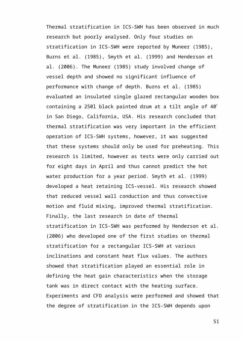
Fig. 3-25: Hot test installation

Observations:

Out of these tests corrective equations were developed by plotting reference British

Standard thermometer readings against thermocouple measured temperatures. Each

thermocouple had an associated equation. Comparison between linear and polynomial

trends were undertaken and showed that a linear regression was sufficiently accurate to

be applied. For each new value read by the thermocouple, the correct value was

determined by its equation.

Errors were quantified statistically by using the coefficient of determination, R2, mean

bias error, MBE, root mean square error, RMSE, as well as Skewness and Kurtosis of

the error histograms and showed acceptable margin of errors. These statistical factors

are further explained in Chapter 4.

Thermocouple positions in the collector

The calibrated thermocouples were used to monitor water temperature at different

positions in the collector. A good distribution of the thermocouples in an inclined ICS-

SWH is essential to determine the temperature profile inside the collector as

stratification causes a variable temperature distribution inside the water tank. Past

studies on ICS-SWH by Grassie et al (2006) suggested a positioning scheme of

thermocouples in ICS-SWH. Temperature profiles observed by Grassie et al (2006)

showed that further thermocouples should be added at the collector’s extremities to

evaluate accurately phenomenon occurring in these zones. A new thermocouple

distribution was therefore developed. Thermocouples were doubled at the top and

bottom part of the middle acrylic clear tube. Both distributions are represented in Figure

3-9 below.

61

Reference

Thermometer

Type K-single

Thermocouples

Data Loggers

Hot water

Constant

temperature

bath

Fig. 3-26: Thermocouple positions and volume control associated, a: Aluminium collector, b:

Stainless-steel Collector (Junaidi et al (2005)).

Control volumes, represented by dashed lines, were assigned to each of the

thermocouples in order to effectively evaluate an average temperature for the water

tank. The temperature profile in the SWH could then be developed using monitored

temperature data.

Thermocouple’s inserts and positions

Clear acrylic tube inserts were used in order to provide support for the thermocouples.

The high resistance to heat distortion and simplicity to insert thermocouples along

acrylic clear tubes made it the best option for this application. Thermocouples were

running through the acrylic plastic tube inserts with multiple slots to expose the

thermocouple tips to the water as shown in Figure 3-10. Tips were fixed in the slot by

silicone.

62

Fig. 3-27: Acrylic plastic tubes inserts with thermocouple slot

Acrylic plastic tubes were placed in the collector through three pipes previously

integrated in the collector design as shown in Figure 3-11.

Fig. 3-28: Acrylic plastic tube inserts in pipes

Positioning of thermocouple tips in the collector

The positioning of thermocouple tips might affect the readings if the thermocouples

appear to be in the flow regime as shown in Figure 3-12. Acrylic tube inserts were

turned to ensure that the tips of the thermocouples were positioned down the central

plane. This was identified as a potential error score when performing a critical review of

previous test regimes employed in ICS-SWH development.

63

Thermocouple tip

Fig. 3-29: Assumption of thermocouple position in the SWH

3.1.2.2 The electrically heated silicone rubber pad

An electrically heated silicone rubber pad was used to control power input simulating

the distribution of solar radiation on the top surface of the collector during laboratory

tests.

Energy distribution of the electrically heated silicone rubber pad

The heat distribution was assumed to be uniform on the collector surface, however, due

to the seasonal variance in sun elevation and positioning, the distribution of solar

radiation on the collector surface is non-uniform. All heat losses due to conduction were

ignored during laboratory experiments. Energy distribution of the electrically heated

silicone rubber pad is represented in Figure 3-13.

Fig. 3-30: Energy distribution of the electrically heated silicone rubber pad

64

Optimising the contact between the electrically heated silicone rubber pad and

collector surface

Aluminium has good heat absorption properties as well as heat transfer properties.

However, the contact between the electrically heated silicone rubber pad and the top

surface of the collector should have minimum air gaps in order to maximise heat

transfer. In order to compare with the methodology used by Grassie et al (2006), tests

reproducing the same conditions were conducted using silicone nodes to fix the

electrically heated silicone rubber pad to the collector’s top surface. Figures 3-14 and 3-

13 show the surface of the pad after the experiment.

Fig. 3-31: Absorber sheet of the ICS-SWH

Fig. 3-32: Silicon paste

The adherence between the electrically heated silicone rubber pad and the collector’s

surface was not optimal and therefore affected the heat transferred to the water.

InfraRed Thermographic images of the pad were taken before removing the silicone

node using a FLIR ThermaCAM thermal camera. Silicone and non-silicone surfaces

were pictured in order to evaluate the effect of silicone on heat distribution and are

represented in Figures 3-16a and b. While a uniform flux through the heating pad was

65

Silicone

Electrically heated

silicone rubber pad

Silicone nodes

expected on both sides, colder spots observed at various positions on the silicone side of

the pad indicated an uneven heating pattern and uniform heat distribution to the non-

silicone side of the pad.

a b

a

Fig. 3-33: Heating pad thermographic images: a. Silicone side (heating side), b. Front side, Scale: C

Figure 3-17a and b showed a more detailed picture of the uneven heating and cooling

pattern of the silicone sided pad. The silicone retains heat when cooled and acts as

insulation when heated.

Fig. 3-34: Heating pad thermographic images: Hot spots (a) and cool spots (b) represent the silicone

welds. Scale: C

In order to improve the initial heating methodology the silicone nodes were removed

and replaced by heat sink compound paste; improving the overall heat transfer between

the two surfaces by two means.

First, a uniform layer of the compound could be applied over the electrically heated

silicone rubber pad attached to the collector top surface, thus providing a more uniform

66

a b

a b

heat distribution and decreasing air interstices between the two surfaces. A second key

factor was the higher thermal conductivity of the heat sink compound of 0.9 W/m.K

compared to the silicone sealant (0.2W/m.K) resulting in a 77% improvement in heat

transferred to the collector.

The electrically heated silicone rubber pad can withstand exposure temperature of up to

230C and has a high emissivity of value 0.86. The fibreglass reinforced silicone rubber

layers sandwich a pre-formed heating element made from fine resistance wires. The

silicone rubber resistant heating pad dimensions were 1000 960mm.

3.1.2.3 Data Loggers

Grant Instrument Squirrel 2020 series, type 1F8, data loggers were used for recording

temperature. In the presence of a temperature difference between the junctions of the K

type thermocouple a small temperature dependent current flows around the circuit. The

measured voltage is converted to a temperature reading through the use of the digital

data loggers using a polynomial relationship for current conversion to temperature

defined by the British Standards (BS EN 60584.1). The 12 Bit data loggers have a

sensitivity specification of 0.1C.

Pyranometer

A Kipp and Zonen BF3 pyranometer was used during the field experiment to measure

hourly horizontal global solar radiation in W/m2, received by the ICS-SWH. It consists

of an array of photodiodes with a computer-generated shading pattern to measure

incident solar radiation mounted on a base covered by a hemispherical glass dome.

Incoming solar radiation lights the photodiodes converting it to a voltage proportional to

the irradiance on that surface which is then read by the computer. Based on Chapter 2, a

45 inclination of the ICS-SWH was used for field tests. The “solar radiation and

daylight Model” developed by Clarke and Muneer (2008) was used to get adjusted solar

radiation for the required inclination.

3.1.3 Experimental considerations

The aim of this section is the identification of the errors due to the assumptions and test

regime that have been made during the experimentation phase.

67

Heated surface

The heat distribution of the electrically heated silicone rubber pad was assumed to be

uniform on the top surface of the heater. All heat losses due to conduction were ignored

during the laboratory experimental tests, however the effects of the heat losses from the

electrically heated silicone rubber pad to the ambient air, the thermal capacitance of the

water storage unit, the glass reflectivity and all other associated losses were taken into

account.

Leakage and pressure inside the collector

The extremities of the pipes from which the acrylic plastic tubes with thermocouples

were inserted were sealed with silicone to avoid any leaks. This might have caused

minor problems due to the build up of pressure inside the collector and thus expansion

of the collector and/or drive the water at the top of the pipes. An expansion water tank

was installed on top of the inlet pipe to overcome such problems.

Departure temperature

Tests were carried out for different controlled heat fluxes provided by the electrically

heated silicone rubber pad. In order to achieve comparable results starting water

temperatures had to be the same for each experiment. Therefore, water in the collector

was purged and replaced by fresh water at approximately 14C after each experiment.

Wind data

Wind speeds were recorded hourly by an anemometer for field tests; however, only an

average wind speed for the location was utilised in calculations as directions were not

recorded. The location of the ICS-SWH was partly sheltered from wind, therefore

decreasing its effect on the glass cover.

3.2 Laboratory experiments

3.2.1 Experimental set up

The equipment set up for the laboratory tests attempted to replicate the previous

experimental schemes of Grassie et al (2006) in order to compare their respective

performance and is described in this section. A total of 22 thermocouples were used to

measure water temperature inside the collector as shown previously in Figure 3-11.

Ambient temperatures inside the laboratory were recorded by two thermocouples while

three others were placed on the glass cover. The electrically heated silicone rubber pad 68

was designed to simulate a constant and uniform heat flux over the flat plate collector

reproducing Edinburgh solar conditions. A variac transformer controlled the power

supply to obtain a measured amount of heat. Tests were carried out for heat fluxes from

100 to 400 W/m2 with increasing intervals of 50 W/m2 at different angles including 0 –

30 – 35 – 45 – 60. Temperatures were recorded at 10 minute intervals over 24 hours,

giving time to reach a state of quasi-equilibrium. The test rig is shown in Figure 3-18

with the circuit diagram of the electrical equipment for control and measurement of the

heat flux in Figure 3-19.

Fig. 3-35: Test rig with control and measurement equipment

Fig. 3-36: Circuit diagram for control and measurement of the heat flux

69

Load / Electrically

heated silicone

rubber pad

Wattmeter

Ammeter

Voltmeter

Variac

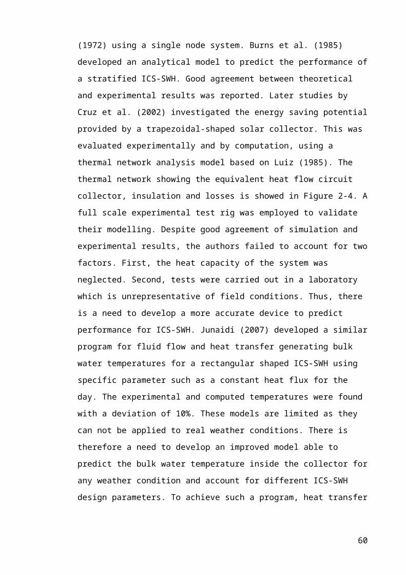
3.2.2 Experiment results

3.2.2.1 General findings

The experimental data obtained replicated and validated Grassie et al’s (2006) work on

stainless-steel ICS-SWH. Equilibrium was experienced after a period of 24 hours when

the peak value of mean water temperature was achieved and all the input heat flux

balanced with net losses. At this stage the water tank temperatures and collector

efficiency tended to a constant value resulting in an asymptotic shape in their profiles.

Every heat flux value has an associated water temperature when equilibrium is reached.

The higher the heat flux imposed, the higher the temperature reached by the collector

but the lower is the overall efficiency as this is the ratio of power output to power input.

In accordance with the results of Grassie et al (2006), an increase of the temperature

stratification with time was observed in the ICS-SWH. The system behaviour also

varied with the angle of inclination. Grassie et al (2006) showed that system

performance differs at various inclination angles and showed that thermal optima

increased by increasing angle of inclination. However, it was suggested that an angle of

45 gave the best overall results when analysing temperatures reached over time, thus

achieving high efficiencies. Results of the research confirmed that the suggestion of an

inclination angle of 45 for the ICS-SWH position was appropriate for Edinburgh.

Further experiments at this inclination showed that the ICS-SWH can work successfully

in a Scottish climate.

3.2.2.2 Aluminium ICS-SWH stratification

Stratification in a water tank is an essential factor for good performance of an ICS-

SWH. It refers to the degree of temperature difference between the top and the bottom

portions of the collector. In order to determine dimensionless stratification,

experimental temperature profiles were scaled and hence the ratio Th / Tbottom was

introduced where Th is the local and Tbottom is the minimum recorded temperature in the

water tank. Stratification profiles for different hours are plotted for a heat flux of

200W/m2 in Figure 3-20. The overall collector temperature increases with time until

reaching steady-state. The first three hours show a rapid increase in temperature

stratification, decreasing later with time until reaching equilibrium.

70

0.98

1.00

1.02

1.04

1.06

1.08

1.10

1.12

1.14

0.0 0.1 0.2 0.3 0.4 0.5 0.6 0.7

HSin, m

T h/T

botto

m

1hr 2hr3hr 4hr5hr 6hr7hr 8hr10hr 16hr

Fig. 3-37: Temperature stratification profile for a 200W/m2 heat flux

Water at a given temperature will settle down at an appropriate height in the ICS-SWH

in accordance with the prevalent density of the fluid. Hot water of low density will

naturally sit in the upper layers while cold water of high density will drop down to the

bottom layers. During the first three hours of the charging process, high temperature

stratification occurs in the ICS-SWH. With time, the temperature of the upper layers is

established and reaches an equilibrium which results in the lower layer achieving a

similar temperature. This therefore decreases the density gradient inside the ICS-SWH.

A temperature stratification profile is thus built up.

This variation in density results in differential buoyancy forces in the fluid causing

convection by gravity. Pressures increases with depth, therefore the pressure within the

collector will experience different pressures at the top and bottom, with the pressure on

the bottom being higher. This difference in pressure causes an upward buoyancy force.

The buoyancy force, , is thus the difference between the forces at the top and bottom

in the collector for one square meter and can be expressed as below:

(3.1)

Where is the density of the fluid at the bottom of the collector (kg/m3)

is the density of the fluid at the top of the collector (kg/m3)

is the vertical length from top to bottom of the collector (m)

is the standard gravity of 9.81N/kg

71

Resulting buoyancy forces within the collector were then calculated. During the

charging period forces increase within the cavity from 3.2N to 8.3N generating

buoyancy driven flows within the cavity. This resulted in an increase in thermal

stratification within the cavity from 2.6C to 3.6C. With time the temperature difference

between top and bottom decreases. This reduction can be associated with a decrease in

buoyancy forces operating within the cavity therefore reducing fluid motion and natural

convection occurring in the collector. After 16hrs, the temperature gradient decreased to

1.9C associated with a buoyancy force of 4.6N. These results are presented in Figure 3-

21.

0.0

1.0

2.0

3.0

4.0

5.0

6.0

7.0

8.0

9.0

1 2 3 4 5 6 7 8 9 10 11 12 13 14 15 16

Time, hrs

Buo

yanc

y fo

rce,

N

0.0

0.5

1.0

1.5

2.0

2.5

3.0

3.5

4.0

Tem

pera

ture

gra

dien

t, °C

Buoyancy forceTemperature gradient

Fig. 3-38: Buoyancy forces with time

The stratification profile was plotted for an average day length of eight hours of ICS-

SWH operation for different wattages. One such profile is shown in Figure 3-22. A

definite relationship between the temperature at any point of the collector and the

applied heat flux was observed. The higher the heat flux imposed the higher the water

temperature ratio Th / Tbottom.

72

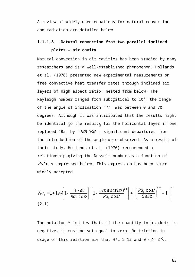
1.00

1.02

1.04

1.06

1.08

1.10

1.12

1.14

0.0 0.1 0.2 0.3 0.4 0.5 0.6 0.7

HSin , m

T h/T

botto

m

100W

200W

400W

Fig. 3-39: Temperature stratification profile after 8 hours of operation

Temperatures are thus dependent on the longitudinal position within the collector,

applied heat flux, and time. A polynomial function for the stratification profile for each

hour was then developed taking heat flux and longitudinal location in the collector as

the main parameters.

3.2.3 Comparison of past and current research

A comparative analysis between the stainless-steel ICS-SWHs previously developed by

Grassie et al (2006) alongside the newly developed aluminium ICS-SWH was

performed in order to validate experiments and to show the benefit of the new ICS-

SWH. The methodology adopted in both studies were first compared followed by

comparisons of experimental results.

3.2.3.1 Test setup comparison

Methodologies adopted in the research were compared with those used by Grassie et al

(2006) to give a viable comparison. The newer collectors were designed and

manufactured with 3mm thick aluminium sheets as compared to the 1.5mm thick

stainless-steel 304-2B ICS-SWH of the same overall dimensions. Grassie et al (2006)

developed two ICS-SWHs; one with and one without fins.

Twenty-two K-type thermocouples were calibrated and used to monitor the temperature

profile inside the aluminium collector compared to twelve thermocouples used in the

73

stainless-steel collectors. Information on the calibration of the thermocouples was not

available for the stainless-steel ICS-SWH experiments.

In order to demonstrate the influence of the number of thermocouples on the accuracy

of results, a first set of calculations using Grassie et al’s (2006) thermocouple positions

for the aluminium collector was implemented. Calculations were then repeated but

taking into account the 22 thermocouples. It was established that the number of

thermocouples did not influence the overall efficiency results.

The second comparison consisted of the methodology for calculating efficiencies. The

heat capacity (Cp) and density () of the water were assumed to be constant by Grassie

et al (2006) contrary to the more accurate method adopted in this research where Cp and

were calculated as a function of the water temperature in the collector. An accuracy

difference of 1% on the overall efficiencies was found by comparing the two methods.

Finally, materials used to attach the electrically heated silicone rubber pad to the

collector top surface were different. Silicone was used by Grassie et al (2006) rather

than a heat sink compound. Two tests were carried out using both materials in order to

compare the conductivity of the two materials resulting in a efficiency difference of 1%

between the two methods. Other parameters which might have affected the accuracy of

the results were the calibration of the thermocouples and data logging equipment.

Based on this methodology the thermal performances of the two finned ICS-SWHs and

benefits of using fins were assessed, compared and adjusted. Results are reported in the

next section.

3.2.3.2 Stratification analysis

The first comparison consisted of a stratification analysis. A dimensionless study of

water temperature according to the distance from bottom to top portions of the collector

was developed with the aim of comparing the thermal stratification of both ICS-SWHs.

Dimensionless temperature of ratio “ ” was plotted in Figure 3-23 against the

dimensionless distance ratio “ ” where is the water temperature at the local point

(K), is the water temperature at the top of the collector (K), is the local length in

the collector (m), is the total length of the collector (m).

74

Figure 3-23 a and b confirm findings from section 3.2.2.2 for the aluminium material

only. It validates that the higher the heat flux applied the higher the stratification in the

ICS-SWH and that the longer the exposure time is the lower is the stratification due to

the buoyancy. These findings are consistent with those of Grassie et al (2006).

0.84

0.86

0.88

0.90

0.92

0.94

0.96

0.98

1.00

0 0.2 0.4 0.6 0.8 1Dimensionless distance

Dim

ensi

onle

ss te

mpe

ratu

re

Stainless-steel -1hr

Stainless-steel -8hr

Aluminium -1hr

Aluminium -8hr

0.76

0.78

0.80

0.82

0.84

0.86

0.88

0.90

0.92

0.94

0.96

0.98

1.00

0 0.2 0.4 0.6 0.8 1Dimensionless distance

Dim

ensi

onle

ss te

mpe

ratu

re

Stainless-steel -1hr

Stainless-steel -8hr

Aluminium -1hr

Aluminium -8hr

Fig. 3-40: Dimensionless temperature “Th/TH” vs dimensionless distance “h/H” at 45 inclination, a: 100W/m2 heat flux input, b: 400W/m2 heat flux input

Another important finding from this figure is the effect of the collector material on

stratification. Steeper stratification curves were found in the stainless-steel ICS-SWH

compared with the aluminium profiles demonstrating a better mixing in the latest ICS-

SWH. This decrease in stratification is explained by the higher conductivity of 75

a

b

aluminium material allowing a more rapid transfer of heat from the top to bottom water

layers. Figure 3.-24 support this finding by depicting the rise in temperature registered

by the thermocouples placed at the top and bottom in the stainless-steel and aluminium

ICS-SWH.

10

20

30

40

50

60

70

80

0 1 2 3 4 5 6 7 8 9 10 11 12 13 14 15 16 17 18 19 20 21 22

Time, hr

Tem

pera

ture

, °C

Fig. 3-41: Water temperature profiles of finned aluminium and stainless-steel ICS-SWHs at 400W,

45 inclination.

Higher water stratification was achieved by the stainless-steel ICS-SWH compared to

aluminium with 9.0°C and 4.5°C difference respectively from the bottom to top of the

collector after an exposure time of eight hours. The aluminium temperature profile

clearly shows that the heat transferred to the water was improved and generated higher

overall water temperatures.

These results indicate that stratification depends upon the incident solar radiation (heat

flux applied to the collector surface), the exposure time and collector material for a

given angle of inclination of the collector.

3.2.3.3 Benefits of introduction of fins in the collector design

In order to quantify the benefit of integrating fins in the collector, a comparison of the

actual rise in temperature of the finned aluminium, finned and un-finned stainless-steel

ICS-SWHs was used. Figure 3-25 compares the results obtained from preliminary

76

Aluminium collector

bottom end

Aluminium collector

top end

Stainless-steel collector

bottom end

Stainless-steel collector

top end

experiments where . is the initial mean water temperature and

is the mean water temperature at any time t.

A rise in temperature of 19.2C, 16.8C and 13.8C was observed after eight hours of

exposure time at 200W/m2 for the finned aluminium, finned stainless-steel and un-

finned stainless steel ICS-SWHs respectively. This corresponded to an improvement of

18% by using fins in the stainless-steel ICS-SWH, and an additional 13% improvement

using the more conductive aluminium.

02468

101214161820

0 1 2 3 4 5 6 7 8

Time. hrs

DT m

, °C

Aluminium_FinnedStainless-steel_FinnedStainless-steel_Unfinned

Fig. 3-42: Water temperature profiles of finned aluminium, finned and un-finned stainless-steel

ICS-SWHs for eight hours of exposure time at 200W.

In order to support the results identified above the overall water temperature of the un-

finned stainless-steel collector was plotted as a function of the finned stainless-steel

ICS-SWH in Figure 3-26., and as a function of the finned aluminium ICS-SWH in

Figure 3-27. These scatter plots have the very specific purpose of demonstrating how

much the “fin” affects water temperature achieved in the collector. It is apparent from

Figure 3-26 and 3-27 that the finned heaters outperform the un-finned by achieving a

higher temperature rise illustrated in Figure 3-26 and 3-27 by the deviation from

the “one to one” straight line relationship. Figure 3-26 and 3-27 also shows that over

time, data points converge; approaching to the “one to one” straight line relationship.

Gradually, un-finned and finned water temperature in the collector tends to reach the

same value; approaching an equilibrium temperature observed for the 100W/m2 heat

flux profile.

77

0

10

20

30

40

50

0 10 20 30 40 50

Finned stainless-steel DTm, °C

Unf

inne

d st

ainl

ess-

stee

l D

T m, °

C

400W200W100W

Fig. 3-43: ICS-SWH water temperature increase: un-finned versus finned stainless-steel

0

10

20

30

40

50

0 10 20 30 40 50

Finned aluminium DTm, °C

Unf

inne

d st

ainl

ess-

stee

l D

T m, °

C

400W200W100W

Fig. 3-44: ICS-SWH water temperature increase: un-finned stainless-steel versus finned aluminium

78

These findings suggest that incorporating fins in the collector results in an increase in

heat transfer, and that using aluminium generates higher overall water temperatures as

shown in Figure 3-26 and 3-27. In a real world application water will be regularly

drawn from the ICS-SWH, not allowing enough time for the water to achieve

equilibrium temperature, early differences in temperature rise is critical for the good

performance of the ICS-SWH.

3.2.3.4 Efficiency improvement

Taking into account all the parameters discussed in section 3.2.3.1, efficiencies were

calculated by the following equation and then corrected. The collector efficiency is the

ratio of the bulk heat collected to the heat available as shown in equation 3.2.

(3.2)

Where is the heat collected at each control volume (W/m2)

is total irradiation from the heating pad (W/m2)

Also expressed as

With (3.3)

Overall efficiency: (3.4)

Where is the control volume associated of the thermocouple “i” (m3), is the heat

flux applied to the system (W), is the specific heat capacity of water associated

with thermocouple temperature (J/kg.K), is the water density associated with the

thermocouple temperature (kg/m3), is the temperature difference between t=j

and t=0s (K) and is the time step (s).

79

To assess the improvement in efficiency of the new aluminium ICS-SWH results of the

above calculations are shown in Figure 3-28.

0.3

0.4

0.5

0.6

0.7

0.8

0.9

0 1 2 3 4 5 6 7 8 9 10 11 12 13 14 15 16Time, hrs

Effic

ienc

y

Al-100WSt-100WAl-400WSt-400W

Fig. 3-45: Aluminium and stainless-steel ICS-SWH efficiency comparison at 45 degree inclination, 100W/400W

Figure 3-28 illustrates two phases in the efficiency curves. Phase one shows a fast

increase in efficiency followed by a regular decrease in phase two. This trend is due to

the thermal mass of the system. It corresponds to the heat stored in the collector material

and the water for a given power applied to the system. Figure 3-28 shows that a longer

period was needed for lower heat fluxes as it takes longer for the material to charge. The

charging stage, associated with the first phase is then dependent on the heat flux

applied. The same figure outlines that the thermal mass of the system is strongly

dependent on the type of material used for the collector. The aluminium collector has a

heat capacity of 17.2 kJ/K compared to 13.3kJ/K for the stainless-steel. The 23%

difference explains the fact that the aluminium collector needs more time to charge for

lower heat flux and vice-versa.

Overall efficiencies obtained from the preliminary analysis for aluminium and stainless-

steel ICS-SWH are presented in Table 3.3. Total efficiencies vary according to the heat

flux in a similar way to that described by Grassie et al (2006). The higher the heat flux

applied to the system, the lower the overall efficiency.

80

1 2

Table 3-6: Stainless-steel vs aluminium overall efficiencies for different heat flux: Note laboratory testsCollector type Heat flux applied Average overall

efficiency100W 200W 300W 400W

Aluminium 77% 77% 66% 63% 71%Stainless-steel 68% 68% 63% 62% 65%

It was also identified that global efficiencies for the aluminium collector were higher at

all heat input regimes compared to stainless-steel. A drop in efficiency was noted

between 200W/m2 and 300W/m2. Tests carried out for 250W/m2 showed an

intermediate value of efficiency.

3.2.4 Discussion of laboratory testing

The purpose of this section was to determine whether the performances of an ICS-SWH

using aluminium as a material were improved by comparison with a previous study by

Grassie et al (2006) utilising a stainless-steel construction device.

This chapter sets out adjustments in the methodology adopted by Grassie et al (2006) in

order to make an appropriate comparison between the two ICS-SWHs. Observations

showed that a generally more accurate and rigorous methodology was adopted in the

experiment of the aluminium ICS-SWH.

The experimental results clearly demonstrated that using aluminium generated higher

overall collector water temperatures and improved heat transfer to the water. The

stratification analysis indicated that this depends upon the incident solar radiation, the

exposure time and collector material, given a constant angle of inclination of the ICS-

SWH.

Findings suggested that incorporating fins in the collector resulted in an increase in heat

transfer of 18% in the stainless-steel ICS-SWH. Using a more conductive material such

as aluminium made an improvement of 13% in water temperature. An overall increase

in the aluminium ICS-SWH efficiency of 6% was found by comparing performances of

both ICS-SWH over an eight hour time period.

The benefit of selecting aluminium for the ICS-SWH was clearly supported by the

current findings showing it out-performing the stainless-steel ICS-SWH. Although the

81

collector was tested in a laboratory with calibrated instruments, the actual performance

of the ICS-SWH in real weather conditions would yield important results on assessing

the viability of the aluminium ICS-SWH. There was therefore a strong imperative for

conducting field tests with the aluminium ICS-SWH.

3.3 Field experiments

To investigate the influence of Scottish weather conditions on the performance of the

aluminium ICS-SWH, extensive field measurements were conducted in Edinburgh

during the summer of 2007.

3.3.1 Experimental test set up

The test rig was located on the roof of Napier University at 15.5m above ground-level

or 113m above sea-level. Due to technical constraints the ICS-SWH was placed facing

143 degrees from north. The electrically heated silicone rubber pad was replaced by a

black paint applied to the absorber plate to improve the solar radiation collection. Figure

3-29 shows the cross-sectional representation of the field tested ICS- SWH while an

illustration of the adopted tests rig is shown in Figure 3-30

Fig. 3-46: Cross-sectional representation of the field tested ICS-SWH

82

Fig. 3-47: Experimental test rig

A simulated roof-structure was used to insulate the sides and back of the ICS-SWH. It

protected the ICS-SWH from the effects of weather by creating a micro-environment

and by decreasing the heat losses from the back of the ICS-SWH. Kingspan insulation

closed-cell polyurethane material was used partially to insulate the bottom of the ICS-

SWH and the back side of the simulated roof-structure as shown in Figure 3-31.

Fig. 3-48: Back insulation of roof simulated box

83

Simulated

“Roof structure”

Cold water

tank

Mineral fibre wool was then placed inside the simulated roof-structure and rigid

insulation was sized and placed on the sides. Wood was then fixed on top of the

insulation as well as a flush system on top of the collector to avoid any water ingress.

Pipes were insulated in order to avoid possible freezing during cold days. Figure 3-32

shows the final installation.

Fig. 3-49: Experimental test rig side insulation

The same 22 K-type thermocouples used for laboratory experiments were connected to

a data-acquisition system to monitor the water temperature inside the aluminium

collector covering middle longitudinal and lateral lines. Other thermocouples were used

to record the absorber plate, the glass cover, the ambient, and the inlet and outlet water

temperatures. A calibrated Kipp and Zonen BF3 pyranometer was used to record solar

radiations at the location of the ICS-SWH while an average wind speed of 3.7 m/s was

recorded next to the location of the ICS-SWH using a WMS302 Vaisala anemometer.

This average data was taken as the reference wind speed in the study. A cold water tank

was placed above the ICS-SWH to feed the collector with fresh cold water and a valve

was used when draw-off of water occurred. A timer was placed to simulate water draw-

off profiles. The angle of inclination of the ICS-SWH was kept at 45, hourly radiation

and ten minutes interval temperatures were recorded for an initial period of three

months.

84

3.3.2 Experiment results

3.3.2.1 Without Draw-Off

Field tests started on 6th June 2007 for an initial period of three months. In order to

identify the performance of the ICS-SWH, data management and analysis were

performed for a typical month of July. Recorded data during the period of the 11th-26th

of July are represented in Figure 3-33 where Tw is the bulk water temperature, Ta is the

ambient temperature, Tp is the plate temperature and Tc is the cover temperature.

0

10

20

30

40

50

60

70

80

11 12 13 14 15 16 17 18 19 20 21 22 23 24 25 26

Dates

Tem

pera

ture

,°C

0

100

200

300

400

500

600

700

800

900

1000

Sola

r rad

iatio

n, W

/m2

TwTaTpTcGlobal solar radiation

Fig. 3-50: Field experiment data

Each day is characterised by a heating and a cooling profile which are dictated by solar

radiation. The higher the incident solar radiation received by the absorber plate, the

higher the water temperature achieved. The decrease in incident solar radiation results

in heat losses from the collector to the surroundings leading to a subsequent decrease in

water temperature. The gradual heating and cooling profiles seen are due to the thermal

mass of the system previously introduced during the efficiency study of laboratory

experiments. The thermal mass is the capacity of a material to store heat. It plays an

important role in the effectiveness of the heating charge and cooling discharge

operations of the collector and the amount of the stored thermal energy. The water

stored in the collector accounts for most of the thermal mass of the system. The high

specific heat 4.18kJ/kg.K and moderate density of 1000 kg/m3 of the water results in a

85

relatively high volumetric capacity of 4180 kJ/m3.K. This shows the ability of a given

water volume to store internal energy while undergoing a given temperature change. Its

low thermal conductivity of 0.58W/m.K also contributes to this effect by slowly storing

or releasing heat. The collector material also contributes to the thermal mass through its

moderate volumetric capacity of 2424 kJ/m3.K, assuming the density of aluminium at

2770 kg/m3 and a specific heat of 875J/kg.K. This results in a thermal mass of 224.7

kJ/K for the collector.

A more detailed picture of a typical day of July is illustrated in Figure 3-34.The

collector is warmed passively by the solar radiation during the day. Heat stored in the

mass is retained and gradually released back during the night illustrated by the cooling

discharge profile.

0

10

20

30

40

50

60

70

80

00 01 02 03 04 05 06 07 08 09 10 11 12 13 14 15 16 17 18 19 20 21 22 23

Time, hrs

Tem

pera

ture

,°C

0

100

200

300

400

500

600

700

800

900

1000

Sola

r rad

iatio

n, W

/m2

TwTaTpTcGlobal solar radiation

Fig. 3-51: One day field experiment data

Figure 3-34 demonstrates the close relationship between the absorber plate and water

temperatures and supports findings on the effect of thermal mass. The absorber plate

absorbs incident solar radiation during the charging operation resulting in an increase of

absorber plate temperature. The absorber plate transfers the heat to the water resulting in

similar temperature profiles. A decrease in incident solar radiation on the absorber plate,

due to shade, resulted in a decrease in absorber plate and water temperatures. However,

as the water volume retained more heat than the absorber plate, higher water

86

temperature occurred during discharge. It was also observed that a significant decrease

in incident solar radiation for a relatively long period of time during the day can lead to

significant losses. However, a short time period would not affect the system

considerably as shown Figure 3-34 between the hours of 12 and 16hrs.

Sky radiation effect on cover temperature

Further analysis of the cover and ambient temperatures in Figures 3-35 showed

significant outcomes. It can be seen that recorded cover temperatures were lower than

ambient temperatures during daytime of the 11th and 15th of July. A possible explanation

for this might be that the effective sky temperature can be about 10-20 degrees Celcius

below ambient temperature at ground level with clear sky conditions and close to or just

below the ambient temperature during cloudy conditions. In order to assess this possible

explanation the clear sky index for the location of the ICS-SWH for those dates were

taken from the BADC (British Atmospheric Data Centre) and plotted against both

temperatures in Figure 3-35.

0

5

10

15

20

25

30

11 12 13 14 15

Day

Tem

pera

ture

, °C

0.0

0.5

1.0

Hou

rly a

vera

ged

clea

r sky

inde

x, k

c

TaTckc

Fig. 3-52: Sky radiation effect on cover temperature with kc as the clear sky index

Both days were recorded as clear sky days from the BADC (2007). The sky acts as a

black body during night-time and during an early morning clear sky, resulting in a cover

temperature lower than the ambient temperature. The energy network illustrating the

87

exchanges between the cover “C” and the absorber plate “P” as well as the ambient air

“A” and the “Sky” node is shown in Figure 3-36.

Fig. 3-53: Energy network for clear sky conditions

Stratification and solar radiation

In order to identify the influence of incident solar radiation on stratification the rise in

temperature registered by thermocouples placed at different locations along the length

of the collector is illustrated in Figure 3-37. Strong evidence of the importance of the

shading effect was found for the hours 11, 12 and 13 where a decrease in stratification

rate was recorded, supporting previous findings. This is due to a sudden decrease in

incident solar radiation on the collector.

0

10

20

30

40

50

60

70

0 1 2 4 5 6 7 8 9 11 12 13 14 15 16 18 19 20 21 22 23

Time, hrs

Tem

pera

ture

, °C

0

100

200

300

400

500

600

700

800

900

Sola

r rad

iatio

n, W

/m2

T2 T5 T9 T12 T13 T16 Global solar radiation

Fig. 3-54: Stratification with time and solar radiation

88

In order to support these findings experimental temperature profiles were scaled to the

ratio Th / Tbottom where Th is the local and Tbottom is the minimum recorded temperature in

the water tank. Dimensionless stratification profiles for different hours are represented

in Figure 3-38 for the same typical day.

1.001.021.041.061.081.101.121.141.161.181.201.221.24

0.0 0.2 0.4 0.6 0.8 1.0Dimensionless distance

Dim

ensi

onle

ss te

mpe

ratu

re

0hr 2hr4hr 6hr7hr 8hr9hr 10hr11hr 12hr13hr 14hr15hr 17hr19hr

Fig. 3-55: Dimensionless longitudinal stratification: Th / Tbottom versus h/L

Temperature stratification decreases gradually over night until 6am, at which time

incident solar radiation starts being collected by the absorber plate. While the overall

collector temperature increases from 7am to 2pm, stratification increases from 7am to

9am then decreasing later with time. This is explained by the buoyancy effect already

discussed in section 3.2.2.2. From 7am high temperature stratification occurs in the

ICS-SWH. At 9am the temperature of the upper layers is established resulting in the

lower layer achieving a narrower temperature range, therefore decreasing the

stratification in the collector. A decrease in de-stratification rate was observed at the 11,

12 and 13hr suggesting that the collector was shaded. This is supported by a sudden

decrease in incident solar radiation on the collector for this period of time shown in

Figure 3-37.

Collection efficiency

It should be noted that the following procedure can be applied to ICS-SWH evaluation;

however it is not truly representative of actual system performance due to its transient or

dynamic nature.

89

The common standard procedure developed by the European Solar Collector and

Systems Testing Group, ESCSTG (1989) was used to measure the effectiveness of the

ICS-SWH. Assuming the collector is operating in a steady state condition, an energy

balance represented by equation 3.5 enables the calculation of the rate of useful energy

gain.

(3.5)

Where is the optical efficiency (transmission-absorption product) of the single

glazed float glass cover

Tw is the bulk water temperature (K)

Ta is ambient air temperature (K)

U is the combined collector heat loss coefficient (W/m2.K).

is the incident solar radiation (W/m2)

Based on equation 3.2 already described in section 3.2.3.4, the collector efficiency is the

ratio of the bulk heat collected to the heat available.

Using equations (3.2) and (3.5), an expression for efficiency was developed in equation

3.6 below.

(3.6)

To avoid negative values of efficiency occurring at early morning or late afternoon a

critical irradiance was introduced. Negative values can occur when incident solar

radiations are lower than the heat losses of the ICS-SWH. This method allowed setting

the heat collection to nil in order to sustain a net energy gain.

(3.7)

As discussed by ESCSTG (1989) equation (3.6) is useful because it can be used to plot

an informative efficiency curve, which predicts collector performance for any operating

point.

90

A constant heat loss coefficient would result in a straight line if efficiency is plotted

against the known operating point. Figure 3-39 illustrates the efficiency curve for the

ICS-SWH experiment data. Based on equation 3.6, the heat loss coefficient of the ICS-

SWH was found to be 4.5 W/m2.K.

0

0.1

0.2

0.3

0.4

0.5

0.6

0.7

0.8

0 0.02 0.04 0.06 0.08 0.1 0.12 0.14 0.16

(Tw-Ta) / I , K.m2/ W

h

Fig. 3-56: Efficiency line for the ICS-SWH studied

As the temperature difference between the bulk water and ambient air increases the

efficiency of collection falls. For any given operating point the efficiency could be

obtained from Figure 3-39 and used to predict the thermal performance of the ICS-

SWH. However, limitations occur by using this procedure for ICS-SWH as it applies

(only) to diurnal system performance. This performance method is applied to the flat

plate collector working in a steady state mode.

3.3.2.2 With Draw-Off

Field tests with draw-off were carried out for the month of August in order to identify

how the ICS-SWH would operate in a building. Based on the literature review,

developed in Chapter 2, McLennan (2006) water consumption for a typical day in

Scotland was taken as reference for an average household of 2.44 persons. The ICS-

SWH was designed as 50 litres or the consumption of one person. Therefore McLennan

(2006) draw-off profiles were adjusted for one person in order to make an appropriate

analysis. Due to experiment restriction caused by the low accuracy of the timer a

minimum flow rate of 0.008l/m2.s was established delivering an average daily hot water

91

consumption of 79l/day/person. McLennan (2006) and the experimental draw-off

pattern established are shown in Table 3-4 below.

Table 3-7: Daily hot water demand profile

Average hot water demand profile by McLennan for 2.44

person

Average draw-off profiles used in experiment

assuming 1m2/personHours Litres/hrs Litres/hrs

1 0 02 0 03 0 04 0 05 1 06 1 07 4 38 23 159 10 7

10 6 411 6 412 4 313 5 314 2 115 2 116 1 117 2 118 4 319 16 1120 13 921 7 522 9 623 5 324 1 0

Total water consumption: 122 Litres/day 79 Litres/day/pers

The flow rate achieved for the experiment of 0.008l/m2.s was found acceptable when

compared with previous research of Duffie and Beckman (1991) suggesting flow rates

of 0.015kg/m2.s or lower flow rates of 0.002 to 0.006 kg/m2.s recently used in Sweden.

Recorded data for two typical days of August are represented below in Figure 3-40.

92

0

10

20

30

40

50

60

70

80

0 3 6 9 12 15 18 21 0 3 6 9 12 15 18 21

Time, hrs

Tem

pera

ture

, °C

Tw ToutT2 T5T13 T16

Fig. 3-57: Stratification in the ICS-SWH and water temperature draw-off

The manufacturing error addressed in section 3.1.1.2 concerning the positioning of the

outlet pipe might affect the flow inside the ICS-SWH when cold water is introduced;

however no specific problems were observed. Results showed that the low flow rate

used for experiments maintained a high level of temperature stratification. A sudden

drop in temperature at the bottom of the tank is recorded at peak demand hours of 19:00

and 20:00. The hot water is tapped and replaced by cold inlet water at the bottom of the

collector therefore decreasing the lower tank water temperature. Strong evidence

suggesting that draw-off increases the overall stratification is shown in Figure 3-40. A

more detailed picture for day two encompassing an interesting set of results is shown in

Figure 3-41.

93

0

2

4

6

8

10

12

14

16

1 2 3 4 5 6 7 8 9 10 11 12 13 14 15 16 17 18 19 20 21 22 23 24

Time, hrs

Dra

w-o

ff, l

0

10

20

30

40

50

60

70

Tem

pera

ture

, °C

Draw off profileTwToutTin

Fig. 3-58: Draw-off profile and performance

It is noticed that the water collected is equal to or above the mean water temperature.

This is merely due to the stratification inside the tank. The lower mean water

temperature achieved after draw-off suggests once more an increase of the overall

stratification in the collector. The average temperatures of the water drawn-off were

recorded as 30.4C, 36.2C, 45.5C and finally 39.7C at peak demand hours of 8:00,

9:00, 19:00 and 20:00 respectively. In order to support the statement that “draw-off

increases the overall stratification” of the collector stratification analysis was carried out

at the two daily peak demand periods and is illustrated in Figure 3-42 and 3-43.

94

1.00

1.05

1.10

1.15

1.20

1.25

1.30

1.35

1.40

0.0 0.1 0.2 0.3 0.4 0.5 0.6 0.7 0.8 0.9 1.0

Dimensionless distance

Dim

ensi

onle

ss te

mpe

ratu

re

5:007:008:0009:0010:0011:00

Fig. 3-59: Ante Meridian dimensionless longitudinal stratification with draw-off: Th / Tbottom Vs h/H

Temperature stratification decreases gradually by night until 5am. The temperature

stratification then increases with time, from 6am to 11am while the overall collector

temperature increases until 2pm. This increase in stratification is due to cold water

being introduced at the bottom of the collector lowering bottom water temperature

therefore increasing the temperature stratification inside the collector. Stratification then

decreases from 12am to 4pm during which time there is no significant water draw-off.

Temperature of the upper layers then starts to be established resulting in the lower layer

achieving a closer equivalent temperature. The temperature stratification then increases

from 5pm to 7pm due to an increase in water being used. An interesting result comes

from the decrease in stratification at 8pm, despite the water being drained-off. This can

be explained by the combination of the large amount of water used at 7pm and the very

low or nil incident solar radiation received by the absorber plate at 8pm in August

resulting in a lower top collector temperature rise.

95

1.0

1.1

1.2

1.3

1.4

1.5

1.6

1.7

1.8

0.0 0.2 0.4 0.6 0.8 1.0

Dimensionless distance

Dim

ensi

onle

ss te

mpe

ratu

re 16:0019:0020:0022:00

Fig. 3-60: Post Meridian dimensionless longitudinal stratification with draw-off: Th / Tbottom Vs h/H

3.3.3 Discussion of field testing

3.3.3.1 Without draw-off

One anticipated finding showed that the higher the incident solar radiation received by

the absorber plate, the higher the water temperature achieved. It was demonstrated that

the thermal mass plays an important role in the effectiveness of the system as it affects

the heating charge and cooling discharge operations of the collector. It was also

observed that a significant decrease in incident solar radiation for a relatively long

period of time can lead to significant losses, therefore positioning of the ICS-SWH is of

primary importance to achieving good performances. It was assessed the cloud cover

should not be neglected as it affects the cover temperature and therefore the final water

temperature output of the ICS-SWH. Finally, the common standard procedure

developed by the ESCSTG (1989) applied to the ICS-SWH suggested that there was a

need for new methods to predict water temperatures achieved and performances of ICS-

SWH.

3.3.3.2 With draw-off

Results demonstrated that draw-off increases the overall thermal longitudinal

stratification in the collector. The manufacturing error of the positioning of the outlet

pipe showed no adverse effect on temperature stratification inside the collector. Average

96

draw-off temperatures recorded at peak demand hours suggest that the ICS-SWH could

cover 55%, 66%, 83% 72% of the hot water demand at 8:00, 9:00, 19:00 and 20:00

respectively based on a delivery temperature of 55°C. A strong relationship between

water drawn-off, water temperature stratification, solar radiation and outlet water

temperature achieved in the collector was reported. It was shown that the ICS-SWH

maintained temperature stratification when draw-off occurred and even improved it.

3.4 Uncertainties and errors associated with measurements

Investigating uncertainties and propagation of errors in experimental procedures is

essential to determine the quality of the data presented. Any likely sources of errors or

problems related to measurement may be categorised under the following two main

categories: equipment error and uncertainty and operation related problems and errors.

A brief analysis of both categories is detailed below.

3.4.1 Equipment error and uncertainty

With any measurement there exist errors, some of which are systematic and others

inherent to the equipment employed. The uncertainty in the resolution is often referred

to as the accuracy of the equipment. Equipment uncertainty and error were analysed and

are reported.

Temperatures in the collector were measured using K-type thermocouples. The

uncertainty in thermocouple measurement after calibration was found to be 0.5C.

Uncertainties associated with calibration were neglected as accurate methods were used

to define the temperature of each thermocouple. An additional uncertainty of 0.1C was

associated with data logger conversion due to its limitation in resolution.

The electrically heated silicone rubber pad and electrical equipment used in the

laboratory experiment for control and measurement of the heat flux had associated

uncertainties. The ammeter and voltmeter used in the laboratory were checked.

Uncertainty in measuring voltage and current were found to be 3% and 1% of

reading values. A wattmeter was used to check the heat flux already measured through

the ammeter and voltmeter. The uncertainty in the power output associated to the

wattmeter was found to be 4.5%. The uncertainty associated with the conversion

efficiency from electrical to heat is difficult to assess as no technical data were provided

by the electrically heated silicone rubber pad manufacturer. An overall uncertainty of

10% in applied heat flux was found acceptable.97

Field experiments equipment used for control and measurements have associated

uncertainties. The BF3 has an estimated uncertainty in global radiation measurement of

5W/m2 at 95% confidence limits. This suggests that 95% of individual readings will

be within the stated limits under normal climatic conditions. The accuracy of the

anemometer was suggested at 0.3m/s for a wind speed less than 10m/s, therefore

appropriate for the ICS-SWH location. The timer used for experiments showed

limitations associated with the draw off profiles. The shortest switch time was of 1

minute therefore restraining the draw-off profile able to be achieved and has an

accuracy of 4 minutes per year.

3.4.2 Operational errors

In addition to the above sources of equipment-related errors, care should be taken to

avoid operational errors highlighted below:

- Operation related problems and errors

- Complete or partial shade of the BF3 from direct sunlight by buildings

- Dust, snow, dew, water-droplets, bird droppings etc.

- Incorrect sensor levelling

Processing errors, human errors or calibration errors are amongst others.

3.5 Concluding remarks

A review of the methodology adopted during laboratory and field experiments was

presented herein. An account of the laboratory experimental set up with its results was

given. ICS-SWH performance was found to be enhanced by using aluminium material.

Determination of stratification dependent parameters, presentably of interest to this

research project was also discussed in order to model stratification for laboratory

conditions. A field experiment was advised and carried out to show the actual

performance of the ICS-SWH in real weather conditions. Parameters such as thermal

mass of the system, incident solar radiation, cloud cover and sky temperature were

found to influence significantly the ICS-SWH performance and are of high interest in

order to model performance of such ICS-SWH for field conditions. Current procedures

measuring the effectiveness of ICS-SWH emphasise a need to predict water

temperatures and performances achieved of ICS-SWH. It was also noted that the ICS-

SWH is able to maintain temperature stratification when draw-off occurred, a crucial

factor to maintain good performance of the ICS-SWH. It was also observed that draw-

off actually increased the overall stratification, thus improving the overall performance 98

of the ICS-SWH. Finally an account of uncertainties and propagation of errors through

both experimental set-ups were addressed.

The work demonstrated in this chapter shows the different parameters influencing the

ICS-SWH and accentuates the need for the development of a thermal program

predicting actual performance of such ICS-SWH.

CHAPTER 4 MODELLING

Modelling is very useful to represent the evolution of fluid flow, temperature and

stratification processes in ICS-SWHs. Micro and macro models were developed to

99

assess these parameters. The macro model assessing fluid flow and heat transfer was

developed using Visual Basic for Applications (VBA). The micro model assessed the

optimum fin spacing using CFD (Computational Fluid Dynamics) Fluent 6.2 software

while meshing was done using pre-processor Gambit 2.2. The macro and micro

models were both used through an iterative time step scheme. Numerical calculations

were developed for the macro model.

4.1 Macro model – Thermal model

As was previously stated in Chapter’s 2 and 3, the common criterion used to measure

the effectiveness of flat-plate SWH using the steady state test procedure proposed by the

ESCSTG (1989) cannot be applied to ICS-SWH as this involves a transient regime.

Direct comparison of measured system performances is relatively straight forward;

however, predicting the performance of an ICS-SWH at another location or with a

different installation configuration is more challenging.

4.1.1 Purpose and Language

A macro model assessing fluid flow and heat transfer in the ICS-SWH was developed

using Visual Basic for Applications (VBA). This macro model is a thermal energy

simulation model which analyses combined heat flux environmental networks within

the ICS-SWH. It was developed to compare the temperature variation in different ICS-

SWH materials, internal water temperature and external weather conditions for a given

aspect ratio. The model generates corresponding bulk water temperature in the collector

with a given hourly incident solar radiation, ambient temperature and inlet water

temperature; thus predicting ICS-SWH performances. Depending on the conditions

applied – laboratory or field – input data will differ.

4.1.2 Capabilities and Limitations

VBA is functionally rich and extremely flexible but it does have some major

limitations. It extends the capabilities of Microsoft Word or Excel through macro

programming language and is widely used by solar energy professionals and engineers.

It can also be used to control almost all functions of the host application (Excel, Word…

functions) and the graphic interface utilisation, like menus and toolbars. VBA is similar

to Visual Basic (VB). However VBA can only run via a host application making it

impossible to operate as a standalone executable. Excel combines a tabular data

acquisition with an inbuilt VBA. In addition to this, some functions in Excel are

100

particularly suited for engineering modelling as described by Liengme (2003) and are

available in VBA as stated by Jacobson (2001). However Excel has two major

limitations as it cannot tabulate more than 65,000 rows, nor graph more than 22,000

data points. Any function of the application or even of the whole operating system is

accessible to the user running a document containing VBA macros making

improvements of the program possible on a continual basis as the code is accessible.

This model was built from scratch hence knowledge based ownership is whole. The

short training time and the lack of special licensing requirements of this kind of

application make the model attractive.

4.1.3 Assumptions

A number of assumptions were made in developing the macro model for instance from

lack of data or in order to reduce computation. Assumptions applying to both laboratory

and field conditions are expressed below:

(a) Transient performance of the system was assumed to be steady state during the small

time steps chosen to solve the thermal network

(b) Thermophysical properties were taken at the film temperature based on Muneer et al

(2003) water and air properties.

(c) Heat loss through the absorber plate to the glass cover was assumed to be equal to

the heat loss from the cover to ambient conditions due to steady state time step.

(d) Heat flow was assumed to be one dimensional.

(e) The absorber plate and glass cover were assumed to be isothermal for the small time

steps chosen.

(f) The plate temperature was started at two degree Celsius above the water temperature

in order to initialise the simulation. This was later recalculated by the programme

through energy balance equations.

(g) The thermal analysis was undertaken for a 45 collector inclination

(h) Dust on the glass cover was assumed negligible

4.1.3.1 For laboratory conditions

Assumptions made to develop the laboratory macro model are given below:

(a) The thermal capacity of the transparent cover was neglected.

(b) Wind velocity was assumed to be 0.1m/s for laboratory conditions.

(c) The sky temperature was assumed equal to ambient temperature.

(d) Stratification inside the collector was first neglected and water temperature was

considered as uniform. Stratification was then modelled.101

Input parameters required for the system to predict ICS-SWH performance are:

(1) Heat flux

(2) Ambient air temperature

(3) Inlet water temperature

(4) Average wind velocity

(5) ICS-SWH characteristics (materials, dimensions, etc…)

(6) Inclination angle of the collector

4.1.3.2 For field conditions

Assumptions made to develop the field macro model are given below:

(a) The absorber plate was assumed to have a constant rate of heat flux for the small

time increments taken by the programme.

(b) An average wind velocity of 3.7m/s was used for the field experiment based on data

recorded on the roof where the ICS-SWH was previously tested.

(c) Radiative heat losses from the glass cover accounted the glass cover and sky

emissivities.

(d) The dry-bulb temperature for part-overcast conditions was assumed as the average

between the overcast and clear sky conditions.

(e) If overcast condition data were not available then the cloud cover was

assumed as part-overcast

(f) Stratification inside the collector was neglected for field experiments; it was thus

assumed that water temperature inside the collector was uniform.

Input required for the system to predict ICS-SWH performance are:

(1) Horizontal global and diffuse irradiation / Sloped global irradiation

(2) Ambient temperature

(3) Inlet water temperature

(4) Wind velocity

(5) ICS-SWH characteristics (materials, dimensions, etc…)

(6) Inclination angle of the collector

(7) Cloud cover

Clear, overcast and part-overcast conditions were differentiated. Sky conditions were set

as: Clear sky conditions:

102

Overcast sky conditions:

Part-overcast sky conditions:

The more detailed and complete the weather information inputs, the fewer error sources,

and thus confidence in the macro model results, might be achieved.

Effects of assumptions were carefully considered in order to ensure that the analysis

was appropriate. Taking these into account, a thermal network and fundamental heat

transfer analysis was developed and then coded through VBA.

4.1.4 Thermal network and fundamental heat transfer analysis

4.1.4.1 Thermal network

The model developed differentiates between unfinned and finned, collector materials

and dimensions of collectors, and was developed on a steady state approach as the water

temperature does not change significantly in very short time intervals. Laboratory and

field macro models have differences as they are subject to different assumptions and

methods of calculations. However, the global thermal network of the ICS-SWH system

will remain the same and is shown in Figure 4-1 below including the water body “W”,

the absorber plate “P”, the cover “C” , the ambient air “A” and the “Sky” nodes.

103

Fig. 4-61: Thermal network of the system

4.1.4.2 Fundamental heat transfer analysis

Transient performance of the system was predicted for a 360 second time interval by

solving the mathematical model consisting of energy balance equations. An iterative

process was developed to solve the thermal network.

The energy balance on the absorber plate at a given instant, assuming steady state

conditions, is given by:

(4.1)

at t=0 (4.2)

104

ccaUrcaU

rpcUcpcU

Sky A

C

P

W

A

mC

wC

pwU

waU

G

Top Cover

Air cavity

Water cavity

(4.3)

Where is the useful energy, G() is the rate of incident solar radiation

transmitted through the glass cover to the absorber plate, is the energy lost from

the absorber plate to the water, is the heat loss from the cover to the surroundings,

is the energy lost from the absorber plate to the glass cover, and is the energy

lost by conduction and convection from the water to the ambient. C is the overall

thermal capacitance of the system composed of , , , , which are the

water, the insulation, the wood, the glass cover, and collector material respectively and

varies for field and laboratory experiments. is the final water temperature at t=i+1

and is the initial water temperature at t=i.

A schematic diagram of heat flux exchanges occurring at the ICS-SWH is shown in

Figure 4-2 below.

Fig. 4-62: Heat flux exchanges occurring at the ICS-SWH

Heat loss from the plate to the cover

These can be expressed by:

105

Heat losses Heat gains

Tw

Air cavity

Water cavity

Ta

Qlosses

Tc

Tp

QUseful

Glass cover

Insulation

Absorber plate

(4.4)

where is the bulk emissivity defined by equation , is the

temperature of the absorber plate, is the temperature of the glass cover temperature,

is the overall U-value between the plate and the cover, is the Stefan-Boltzmann

constant and is the convective heat transfer coefficient between inclined parallel

plates with a slope from the absorber plate to the glass cover. Based on the work of

Hollands et al (1976) the following relationship of for inclined cavities was

developed:

(4.5)

Where is the thermal conductivity of air at film temperature and L is the

characteristic length. The notation * implies that, if the quantity in brackets is negative,

it must be set equal to zero.

Heat loss from the cover to the surroundings

Losses to surroundings will differ whether the models compute laboratory or field

conditions. Both are expressed below respectively:

Laboratory conditions:

(4.6)

Field conditions:

(4.7)

106

where is the external convection from the glass cover to ambient, is the sky

temperature, is the ambient temperature, is the glass cover emissivity and is

the bulk emissivity of equation where is the emissivity of the sky.

The following correlation was suggested by Duffie and Beckman (1974) for convection

occurring on a collector surface where is the wind speed.

(4.8)

According to CIBSE guide A (2006), a value of 0.1m/s of can be used to represent

convective velocity in a closed room adequate for laboratory tests. A value of 3.7m/s,

based on experimental observations, for field tests based in Edinburgh was assumed.

As stated in the literature, is the sky temperature and is assumed equal to for

laboratory conditions. However, for field tests the sky is acting as a black body during

night and during clear sky conditions in early morning.

The sky temperature was then determined by using the expression developed by Berdahl

and Martin (1984) in equation (4.9) below where the sky temperature is related to the

dew point temperature, , ambient temperature, , and time relative to midnight, .

(4.9)

The sky emissivity was calculated by integrating Cucumo et al’s (2006) equation (4.10)

of clear sky emissivity, , into Santamouris and Asimakopolous’s (1996) equation

(4.11) for sky emissivity in the transparency window, .

(4.10)

With

107

Where is the atmospheric emissivity in the transparency window for clear sky

condition and is the global emissivity.

The sky emissivity in the transparency window, , was then calculated by using the

final expression by Santamouris and Asimakopolous (1996) expressed below:

(4.11)

Where n is the total opaque cloud amount; 0 for clear sky and 1 for overcast sky.

A bulk emissivity, , taking into account the sky and glass cover emissivity of

equation was then introduced to calculate the radiative heat losses from the

glass cover to the surrounding for field experiments.

Dew-point and ambient temperatures relationship were developed for Edinburgh, based

on one year data from the British Atmospheric Data Centre (BADC). This data is

plotted in Figures 4-3 and 4-4 from which the following relationships were developed

for the different types of sky.

For clear days: (4.12)

For overcast days: (4.13)

It was assumed that part-overcast dew-point temperature was the average between clear

and overcast conditions resulting in a dew-point expression below:

(4.14)

108

y = 0.71x - 0.79R2 = 0.88

-10

-5

0

5

10

15

20

-10 -5 0 5 10 15 20 25

Ambient temperature, °C

Dew

-poi

nt te

mpe

ratu

re, °

C

Fig. 4-63: Dew-point and ambient temperatures relationship for clear days

y = 0.82x - 0.81R2 = 0.80

-10

-5

0

5

10

15

20

25

-10 -5 0 5 10 15 20 25

Ambient temperature, °C

Dew

-poi

nt te

mpe

ratu

re, °

C

Fig. 4-64: Dew-point and ambient temperatures relationship for overcast days

Heat loss from the absorber plate to the water

The heat transfer to the water is mainly a convective process thus conduction was

neglected. The heat loss from the absorber plate to the water is expressed below:

(4.15)

109

where is the temperature of the absorber plate, is the water temperature at t = i,

is the overall U-value between the absorber plate and the water. A Nusselt

expression for trapezoidal-shaped ICS-SWH based on Fuji and Imura (1972) and

adapted by Cruz et al (1999 & 2002) to evaluate expressed as:

(4.16)

Where and , for Edinburgh conditions, is the thermal

conductivity of water at film temperature and L is the characteristic length. A visual

description is shown in Figure 4-5 below.

Fig. 4-65: Geometric parameters of the ICS-SWH (blue nodes denote fluid temperature

measurements locations)

Heat loss from the water to the ambient

(4.17)

110

where is the water temperature at t = i, is the ambient temperature and is the

overall U-value between the water to the ambient through the box, developed as:

(4.18)

Where is the resistance of the insulation material which will vary between laboratory

and field installations, and is the resistance occurring at the box surface in contact

with the wind.

Heat loss from the fins to the water

The inclusion of extended heat transfer surfaces (fins) into the design resulted in an

increase in heat transfer to the water. Ideally the fin material should have a large thermal

conductivity to minimize temperature variations from its base to tip. Four fins of

straight, rectangular uniform cross sectional area were used for the design. Each fin was

attached to a base surface of temperature called plate temperature and extends

into fluid temperature as described in Figure 4-6.

Fig. 4-66: Straight rectangular fins of uniform cross section and energy balance for an extended

surface

Based on the work of Incropera and Dewitt (2001), a new model was developed using

an elemental strip method to determine the heat transferred from the fin to the water

assuming an adiabatic tip condition ( ): . The fin temperature

distribution along the length was determined by the following formula:

111

Tp

(4.19)

Where

= cross sectional area ( )

= perimeter

= strip position

d = depth of the fins

The fin heat transfer rate per strip can be expressed as:

(4.20)

Where fin area

number of fins

strip length taken equal to for modelling.

The heat transfer to the water is mainly a convective process. Muneer et al (2003) used

the equation of Churchill and Chu (1975) incorporating the following regression

assuming a uniform heat flux:

(4.21)

Where with as the inclination angle of the collector and d as the

depth of the fins.

The effective length of the fin was defined when 90 percent of the actual

was achieved - as only 90 percent of the heat was assumed to conduct through the fins

and is represented in Figure 4-7 below.

112

0.0

0.1

0.1

0.2

0.2

0.3

0.3

0.4

0.4

0.5

0.0 0.1 0.2 0.3 0.4 0.5 0.6 0.7 0.8 0.9 1.0

Dimensionless fin length, x /d

Dim

ensi

onle

ss fi

n te

mpe

ratu

re,

(Tp-

T f,x

)/(T p

-Tw)

Aluminium collector-3mmAluminium collector-1.5mm

Stainless-steel collector-1.5mm

Fig. 4-67: Dimensionless fin temperature versus fin length

The total heat transferred through the fins to the water was calculated using the

effective length of the fin. The quantity , expressed below was calculated by

adding up the fin heat transfer rate per strip until reaching the limit of effective

length.

(4.22)

An improvement factor (IF) was introduced representing the improvement achieved by

using fins in the ICS-SWH over an un-finned collector and is expressed in equation 4.23

below.

(4.23)

Calculation of the bulk water temperature

Using the equations developed above, an iterative computer program was developed

using VBA with initial conditions of and set as:

113

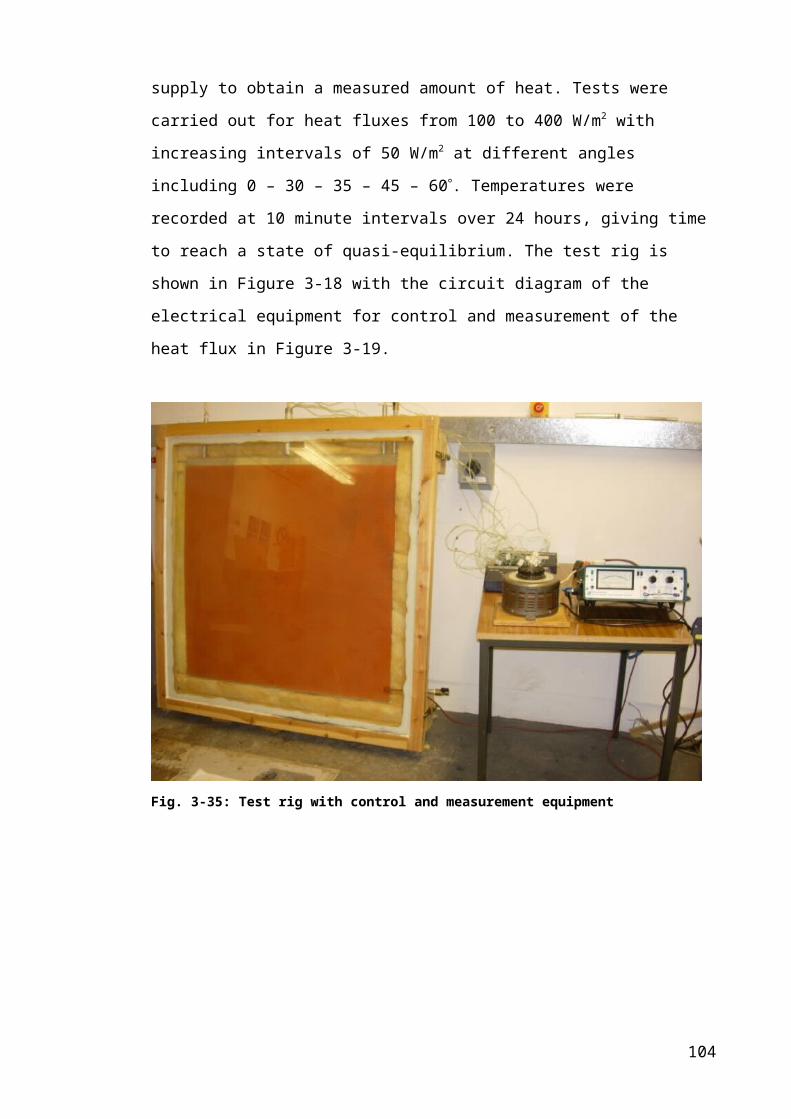
Using equations (4.2) and (4.3), expressions for and for t=0 were developed

below in equations (4.24) and (4.25). The glass cover temperature at t=0 is a function of

the assumed value of absorber plate temperature.

for laboratory conditions (4.24)

for field conditions

(4.25)

Iterations were made until a balance was obtained between heat losses. The program

finally output the glass cover temperature ‘ ’ and the absorber plate temperature ‘ ’.

Heat fluxes in the network are calculated in the macro and using equation (4.1) a

transformed equation (4.26) can be developed to calculate the water temperature rise:

(4.26)

An interval of one hour was taken to display results. After each interval the value of the

cover, absorber plate and water temperature were calculated and used as the input for

the next time step. The cycle was repeated for 24 hour time increments.

If the option “NO” fins is activated, then is automatically set to zero, then fins are

not taken into account into the calculations.

4.1.5 Modelling stratification for laboratory conditions

Stratification in a water tank is an essential factor for the good performance of an ICS-

SWH. This section explores the modelling of stratification inside an aluminium ICS-

SWH for laboratory conditions.

114

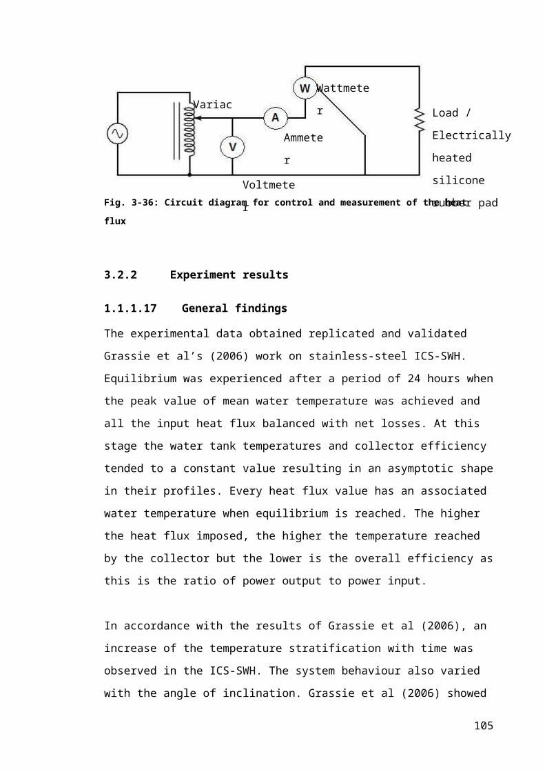
Water temperatures within the collector were observed, in Chapter 3, to be dependent

on the longitudinal position, imposed heat flux, and exposure time. Using experimental

data, a polynomial function for the stratification profile at each hour was developed

using heat flux and longitudinal position in the collector as the main parameters. In

order to obtain a generalised equation for any heat flux, dimensionless temperature, ,

and dimensionless length, , were calculated and plotted for each temperature

measurement location for the aluminium ICS-SWH on an hourly interval. This is shown

in Figure 4-8.

-0.08

-0.06

-0.04

-0.02

0.00

0.02

0.04

0.0 0.1 0.2 0.3 0.4 0.5 0.6 0.7 0.8 0.9 1.0

h*=h/H

=

(Th-

Twb)

/Tw

b

100W

200W

400W

Fig. 4-68: Dimensionless temperature stratification after 8 hours

Polynomial functions were developed from Figure 4-8 for each wattage as defined

below:

(4.27)

A single function was then developed incorporating the change of stratification with

position and heat flux. The following equations were developed to produce a

temperature stratification profile for an average eight hour day. Polynomial functions

for heat flux of 100, 200 and 400W/m2 are expressed below:

(4.28)

(4.29)

115

(4.30)

A final overall expression was then developed for each hour as a function of the heat

flux input and the longitudinal position in the collector. The expression for the stratified

temperature at the end of eight hours of operation is given as:

(4.31)

Where a, b and c are the variation of the polynomial coefficient with heat flux for each

hour. Coefficients were noted and modelled in a more generalised function and are

provided below:

(4.32)

(4.33)

(4.34)

The same approach was used for each hour.

Using the previously developed macro model for laboratory conditions; polynomial

functions were added to the macro model to compute water temperature stratification

with height. The initial laboratory macro model was able to generate corresponding bulk

water temperatures in the collector with a given hourly incident solar radiation, ambient

temperature and inlet water temperature.

The new model was able to compute the bulk water temperature variation in different

ICS-SWH collectors for a given aspect ratio and to evaluate temperatures at various

points in the collector (temperature stratification) based on the mean water temperature

given by the macro model and the total time of exposure.

Results comparing computed with experimental stratification are discussed in section

4.1.7.2.

116

4.1.6 Digital simulation flow chart

Input Heat Flux or Solar radiation, G()

Calculation of Tw from QUseful

Update time step, t: i = i + 1

i = 10*

END

Checki

Update Tp and Tc i = i + 1

Calculation of Uca and Upc

Inlet water temperature, Tw

Initialisation of Tp and Tc

Ambient temperature, Ta

Cloud cover, CC

Calculation of Tdp

Calculation of TSky and Sky

Air properties at film temperature, Tfa

Wind velocity Vw

Cover and plate emissivity, c, p

Water properties at film temperature Tfw

Calculation of QFins

Calculation of QUseful

Calculation of Tp and Tc (eq. 4.24 – 4.25)

Calculation of Upw

Calculation of Uwa

Checki = 10

i = 10

i < 10

i < 10*

117

4.1.7 Computational and experimental data comparison

4.1.7.1 Laboratory results

Results for finned collectors

Figures 4-9 and 4-10 show the simulated heat transfer rate through the fins and the fin

temperature through the fin length respectively. The fins were used to enhance heat

transfer between the material and the adjoining fluid. The heat transfer rate was

increased by employing different fins configuration as demonstrated in Figure 4-9. The

thermal conductivity of the fin material has a strong effect on the temperature

distribution along the fins (Figure 4-10) and therefore influences the degree to which the

heat transfer rate is enhanced as shown in Figure 4-9. Ideally the fin material should

have a large thermal conductivity to minimise temperature variations from its base to its

tip.

0.0

0.1

0.2

0.3

0.4

0.5

0.6

0.7

0.8

0 4 8 12 16 20 24 28 32 36 40 44 48

Fin length x, mm

Fin

heat

tran

sfer

rate

, W

Aluminium collector-3mmAluminium collector-1.5mmStainless-steel collector-1.5mm

Fig. 4-69: Simulated fin heat transfer rate

118

51.30

51.35

51.40

51.45

51.50

51.55

51.60

0 5 10 15 20 25 30 35 40 45 50

Fin length x, mm

Fin

tem

pera

ture

, °C

Aluminium collector-3mmAluminium collector-1.5mmStainless-steel collector-1.5mm

0.10,AL-3

0.10 , AL-1.5

0.10 ,ST-1.5

Fig. 4-70: Simulated fin temperature drop where is the excess

temperature achieved assuming 90% of heat is conducted through the fins.

Fin length effectiveness, and consequently heat transfer rate are enhanced by choosing a

material with high thermal conductivity; such as aluminium. It was also enhanced by

increasing the thickness of the fin, increasing at the same time the surface in contact

with water. The optimum effective length of the fin was defined earlier when 90 percent

of the actual was achieved. The optimum effective length for the

aluminium collector fin of 3mm and 1.5mm thickness, and stainless-steel of 1.5mm

thickness were found to be 33.67, 31.50 and 12.62mm respectively; equating to an

effective fin utilisation of 67.3%, 63% and 25.3%, based on their respective optimum

effective length.

Similarly, a higher fin heat transfer coefficient is achieved using the higher conductivity

material and greater material thickness. Indeed, by increasing the thickness a greater

amount of heat was transferred through the fins’ length to achieve improved rates of

heat transfer to the bottom of the collector as shown in Figure 4-11.

119

48.0

98.0

148.0

198.0

248.0

298.0

348.0

398.0

448.0

0 4 8 12 16 20 24 28 32 36 40 44 48Fin length x, mm

Fin

heat

tran

sfer

coe

ff., W

/m2 .K

Aluminium collector-3mmAluminium collector-1.5mmStainless-steel-collector 1.5mm

Fig. 4-71: Simulated fin heat transfer coefficient

Results showed that the higher the heat flux applied to the system, the higher the fin

heat transfer rate achieved. However, the fin heat transfer rate decreases along the

length until reaching an asymptotic value corresponding to the heat flux applied. Figure

4-12 reveals another typical trend showing that with time the fin heat transfer rate

decreases. This is because with time the collector water temperature increases thus

reducing heat transfer from the fins as the water approaches a temperature equilibrium

with the external heat flux applied to the system

0.0

0.5

1.0

1.5

2.0

2.5

0 4 8 12 16 20 24 28 32 36 40 44 48

Fin length x, mm

Fin

heat

tras

nfer

rate

, W

Fig. 4-72: Simulated fin heat transfer rate with time – Aluminium 3mm SWH

120

1 hr 5hrs 10hrs 15hrs 20hrs

A fin efficiency was then calculated to evaluate the fin performance. Referring to the

work of Incropera and Dewitt (2001), for a straight fin of uniform cross section and an

adiabatic tip condition the fin efficiency was defined by:

(4.35)

Where .

The fin efficiencies were plotted in Figure 4-13 for the three ICS-SWH aluminium and

stainless-steel fins to see the improvement in efficiency from using a higher

conductivity material and by increasing the fin thickness. Higher efficiencies were

achieved for the aluminium material with a 3mm fin thickness.

0

20

40

60

80

100

0 5 10 15 20 25 30 35 40 45 50

Fin length x, mm

hf, %

Aluminium collector-3mmAluminium collector-1.5mmStainless-steel collector-1.5mm

Fig. 4-73: Simulated fin efficiency

The improvement factor (IF) decreases with time while the water temperature increases.

Indeed decreases while increases with time and are related to the water

temperature and the IF. These results are interrelated. A comparison between different

types of fins was made for an input temperature of 22.1C and a heat flux of 100W/m2

applied to the system. Results are presented in Table 4.1 below.

121

Table 4-8: Overall improvement factor for given parameters

Material Fin thickness, mm Overall IF

Aluminium 3 1.14

Aluminium 1.5 1.10

Stainless-steel 1.5 1.04

Unfinned - 1.00

By increasing the thickness of the fins the overall IF improved by 3.5%, while by

changing the material to a more conductive material the IF improved by 5.5%. The

improvement factor measuring the fin performance showed that, overall, a higher

performance was achieved for the aluminium ICS-SWH with a 3mm fin thickness.

Comparison of the digital simulation and laboratory results

A comparison was undertaken between the computational results from the model and

the actual experimental data. Simulated and computed efficiency of the aluminium ICS-

SWH achieved with time for 400W/m2 was plotted in Figure 4-14 and show a good

empirical correlation.

The comparison of the water temperatures achieved experimentally and numerically

was plotted in Figure 4-15 for the three ICS-SWHs. Good correlations were observed

for all the ICS-SWH types.

01020304050607080

0 2 4 6 8 10 12 14 16 18 20 22Time, hrs

h, %

400W_Experimental400W_Simulation

Fig. 4-74: ICS-SWH efficiency with time for 400W/m2 heat flux applied

122

0

5

10

15

20

25

30

35

40

0 2 4 6 8 10 12 14 16

Time, hrs

DT m

, °C

Finned Auminiuml_ExperimentalFinned Aluminium_SimulationFinned Stainless-steel_ExperimentalFinned Stainless-steel_Simulation

Unfinned Stainless-steel_ExperimentalUnfinned Stainless-steel_Simulation

Fig. 4-75: Computational and experimental comparison for 250W/m2 heat flux

Computed data were plotted as a function of experimental data in Figure 4-16 to

examine the validity of the simulation. It was demonstrated that experimental and

computer simulation results are in good agreement as they follow a 1:1 relationship with

a 10% over prediction in the modelled value.

0

20

40

60

80

0 20 40 60 80

T measured, °C

T co

mpu

ted,

°C

Fig. 4-76: Computed vs Experimental water temperatures

123

However, a proper validation of the results by statistical methods and extreme range

tests was carried out in order to improve confidence in the findings.

Statistical measures used for evaluation of the model

In order to evaluate the performance of each set of models, the following statistical

indicators were employed:

- Slope of the best-fit line

- Coefficient of determination (R2)

- Mean bias error (MBE)

- Root mean square error (RMSE)

- Skewness

- Kurtosis

The slope of the best-fit line between the computed and measured variable is desirably

equal to one. Slope values exceeding one indicate over-estimation; while slope values

less than one indicate under-estimation of the computed variable.

The coefficient of determination, R2, is the ratio of explained variation to the total

variation. It lies between zero and one. A high value of R2 indicates a lower unexplained

variation and is desirable. R2 is often used to judge the adequacy of a regression model

but it should not be the only criterion for choosing a particular model.

(4.36)

Where = computed value

= mean value

= measured value

= number of points

The mean bias error, MBE, provides a measure of the trend of the model, whether it has

a tendency to under-predict or over-predict its modelled values. Positive values of MBE

indicate under estimation while negative values imply over estimation by the proposed

model. A MBE nearest to zero is desired. It is given by the following equation:124

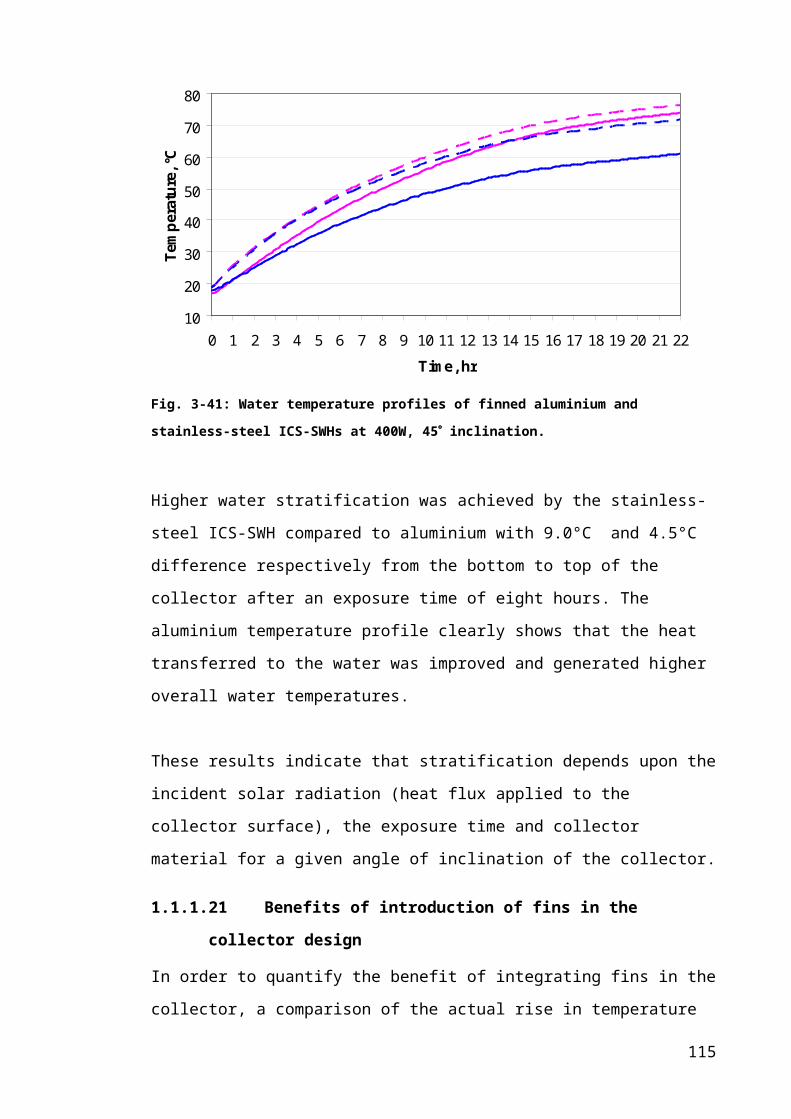
(4.37)

Where = number of points

The root mean square error, RMSE, gives a value of the level of scatter that the model

produces by providing a comparison of the actual deviation between the predicted and

the measured values. Since it is a measure of the absolute deviation, RMSE is always

positive. A lower absolute value of RMSE indicates a better model.

(4.38)

Skewness represents a measure of the lack of symmetry in a distribution.

A distribution is symmetric or normal if it looks the same to the left and right of the

centre point, resulting in skewness statistic of zero value for perfect symmetry. This

would indicate a robust model. A positively skewed distribution tails off to the high end

of the scale while negative skew tails off the low end of the scale.

Kurtosis is defined as a measure of the degree of peakedness in the distribution, relative

to its width. The kurtosis statistic will be zero for a normal distribution, positive for

peaked distributions and negative for flat distributions. A peaked distribution of the

errors is highly desirable. A high positive value of kurtosis suggests that there are fewer

outliers in the estimation.

The six statistical indicators detailed above were used in the research to quantitatively

evaluate the performance of the model. These were calculated using a macro within

VBA and are summarised in Table 4-2. Extreme range tests were also used to evaluate

the reliability of the laboratory macro model to predict bulk water temperature in the

ICS-SWH.

Table 4-9: Statistical indicators values – Total Data

Statistical indicator Values125

Slope 1.01

R2 0.996

MBE (C) -0.30

RMSE (C) 1.00

Skewness (C) -0.79

Kurtosis 3.21

The slope of the best fit line between computed and measured temperature was found to

be equal to 1.01 suggesting a slight over estimation of the computed variable. The high

value of R2 indicates a low unexplained variation showing a good capability of the

regression model. The MBE value of -0.30 shows that the model has a tendency to over

predict its computed values. The low RMSE value of 1.0 shows an acceptable actual

deviation. The low negative skewed distribution tends to the lower end of the scale.

However, its low value of - 0.79 indicates a robust model. The positive kurtosis of 3.21

indicates a peaked distribution of the errors suggesting that there are low outliers in the

estimation.

Finally extreme range tests were undertaken to show the credibility of the model. For a

period of eight hours at constant heat flux of 50 and 600W/m2 good close fitting curves

of computed and experimental data were achieved with very low MBE and RMSE

values of -0.43 and 0.53 respectively suggesting a robust model.

Statistical and extreme range results validated the accuracy of the model to compute

bulk water temperature.

4.1.7.2 Stratification - model results

Results

This section explores the validity of the model predicting stratification inside the ICS-

SWH by comparing computed results with experimental data. The simulation was

carried out for a wide range of heat inputs (50, 100, 150, 200, 250, 300, 350, 400 and

600W) for a period of eight hours simulating a typical day of operation. Computed

water temperatures at any given height were plotted as a function of experimental data

to examine the validity of the simulation. It was demonstrated that experimental and

126

computer simulation results were in good agreement as they followed a 1:1 relationship

shown in Figure 4-17.

0

10

20

30

40

50

60

70

80

0 10 20 30 40 50 60 70 80

T measured, °C

T co

mpu

ted,

°C

Fig. 4-77: Computed vs Experimental stratification after 8 hours of operation for all heat inputs

It is observed in Figure 4-18 that variation between experimental and computed results

data occurs during extended (22hr) model validation and experimental testing regime

displayed graphically by a deviation from the uniform 1:1 relationship. It suggests that

as temperatures increase towards boiling, bulk fluid movement is breaking down the

stratification. Based on the assumption that water temperatures to be achieved in a

Scottish climate are unlikely to exceed 70C and that a typical solar heating day would

be of eight hours or less make this model suitable for Scottish weather conditions.

127

0

10

20

30

40

50

60

70

80

90

100

0 10 20 30 40 50 60 70 80 90 100

T measured, °C

T co

mpu

ted,

°C

Fig. 4-78: Computed vs Experimental stratification after 22 hours for all heat inputs

The stratification model was developed using experimental data for 100, 200 and

400W/m2. A detailed picture of the stratification model results for a heat input of

200W/m2 applied to the system for up to eight hours is showed in Figure 4-19. Each

wattage followed a 1:1 relationship showing good agreement between experimental and

computed data.

128

0

10

20

30

40

50

0 10 20 30 40 50

T measured, °C

T co

mpu

ted,

°C

Fig. 4-79: 200W/m2 data - Computed vs Experimental stratification after 8 hours of operation

Statistical measures used for evaluation of the model

The previously detailed statistical indicators were used to evaluate the performance of

the model to predict temperature stratification in the ICS-SWH and are summarised in

Table 4-3.

Table 4-10: Statistical indicators values – Total Data

Statistical indicator Values

Slope 1.00

R2 0.99

MBE (C) -0.47

RMSE (C) 0.83

Skewness (C) -0.17

Kurtosis 3.39

The slope of the best fit line was found to be equal to one suggesting no over or under

estimation of the computed variable. The high value of the coefficient of determination

(R2) indicates a low unexplained variation and thus good correlation. The MBE value of

-0.47 shows that the model has a tendency to over predict its computed values by nearly

half of one degree Celsius. The low RMSE value of 0.83 suggests a satisfactory actual

deviation. The low skewness negative value of -0.17 is close enough to zero to indicate

129

a robust model. The positive kurtosis value of 3.39 indicates a peaked distribution of the

errors suggestive of fewer outliers in the estimation.

Different heat inputs outside the normal experimental range were then simulated in

order to validate the model. Results for 50, 150, 250, 350 and 600W/m2 were plotted for

a typical day of eight hours in Figure 4-20. The figure confirmed a good agreement

between experimental and computed data following a 1:1 relationship with an MBE and

RMSE of 1 and 1.4 respectively and a slope and coefficient of determination of 0.97

suggesting an under estimation of the computed variable, validating the stratification

method used.

0

10

20

30

40

50

60

70

0 10 20 30 40 50 60 70

T measured, °C

T co

mpu

ted,

°C

50W150W250W350W600W

Fig. 4-80: Validation of the model - Computed vs Experimental stratification after 8 hours of

operation

4.1.7.3 Field - model results

This section explores the validity of the model to generate and predict water bulk

temperature inside the ICS-SWH for field weather conditions. Simulations were

undertaken for an aluminium collector of 3mm thickness tilted at an inclination angle of

130

45 in order to compare computed results with experimental results undertaken on the

roof of Napier University as described in Chapter 3.

Results

In accordance with laboratory computed data, the role of extended heat transfer fins was

demonstrated and showed good improvement by achieving higher bulk water

temperatures.

A first analysis carried out for a period of five days (11th- 15th July 2007) explores the

validity of the model to predict bulk water temperature inside the ICS-SWH by

comparing computed results with experimental data. Results are plotted in Figure 4-21.

0

10

20

30

40

50

60

70

1 7 13 19 1 7 13 19 1 7 13 19 1 7 13 19 1 7 13 19Time, hrs

Tem

pera

ture

, °C

0

100

200

300

400

500

600

700

800

900

1000

Sola

r rad

iatio

n, W

/m2

Tw-Experimental Tw-ComputedTp-Experimental Tp-ComputedTa Solar radiation

Fig. 4-81: Computed and experimental data for a five day period in July 2007

Figure 4-21 shows that similar to experimental field results, computed results show that

each day is characterised by a heating and a cooling profile which are dictated by solar

radiation. The higher the incident solar radiation received by the absorber plate, the

higher the water temperature computed. It was observed that gradual heating and

cooling profiles due to the thermal mass of the system were experienced due to the

consideration of thermal mass in the macro model. However, a lower cooling rate of the

modelled values was observed each day. This could be explained by the propagation of

131

errors and uncertainty by the use of regression analysis and assumed weather data;

resulting in a decrease in accuracy of the model.

It was also observed in Figure 4-21 that experimental water temperature was followed

very closely by predicted water temperature although it showed a slight over-estimation

by the proposed model. In order to examine the validity of the simulation computed data

were plotted as a function of experimental data in Figure 4-22.

0

10

20

30

40

50

60

70

0 10 20 30 40 50 60 70

T measured, °C

T co

mpu

ted,

°C

Fig. 4-82: Computed vs Experimental for a five day period in July 2007

It was demonstrated that experimental and computer simulation results were in good

agreement as they followed a 1:1 relationship shown in Figure 4-22. Statistical

indicators were then used to evaluate the performance of the model for those five days

and are resumed in Table 4-4.

Table 4-11: Statistical indicators values

Statistical indicator Values

Slope 1.03

R2 0.97

MBE (C) -1.27

RMSE (C) 2.19

Skewness (C) 0.86

Kurtosis 0.42

132

The slope of the best fit line suggests a slight over estimation of the computed variable.

The high value of R2 indicates a low unexplained variation showing a satisfactory

accuracy for the regression model. The MBE value of -1.27 shows that the model has a

tendency to over predict its computed values. The RMSE value of 2.19 shows an

acceptable actual deviation. The low positive skewed distribution trends to the high end

of the scale and indicates a robust model. The positive low kurtosis indicates a peaked

distribution of the errors suggesting that there are low outliers in the estimation.

A study of the effect of wind velocity on the bulk water temperature was carried out and

is illustrated by Figure 4-23 where V0, V2, V4 and V6 represents the wind velocity

values of 0m/s, 2m/s, 4m/s and 6m/s respectively. The higher the wind velocity, the

higher the heat losses resulting in lower bulk water temperature showing the influence

of wind speed on overall performance. Thus, having accurate wind speeds would result

in more accurate bulk water temperatures. The more data input, the more accurate

becomes the model.

20

25

30

35

40

45

50

55

60

65

70

0 8 16 0 8 16 0 8 16 0 8 16 0 8 16Time, hrs

Bul

k w

ater

tem

pera

ture

, °C

V0 V2V4 V6

Fig. 4-83: Simulated effect of wind velocity on water temperature for a five day period in July 2007

where V0, V2, V4 and V6 represents the wind velocity values of 0m/s, 2m/s, 4m/s and 6m/s

respectively

A second simulation was carried out over a period of 50 days (7th June - 27th July 2007)

in order to determine the validity of the model to predict bulk water temperature for an

133

extended period. Total computed and experimental data are plotted in Figure 4-34 at the

end of the chapter.

Computed data were then plotted as a function of experimental data to examine the

validity of the simulation. It was demonstrated that experimental and computer

simulation results were in good agreement as shown in Figure 4-24.

0

10

20

30

40

50

60

70

0 10 20 30 40 50 60 70

T measured, °C

T co

mpu

ted,

°C

Fig. 4-84: Computed vs Experimental for a 50 day period in July

The same statistical indicators were then used to evaluate the performance of the model

to predict bulk water temperature in the ICS-SWH for the extended 50 day test and are

given in Table 4-5.

Table 4-12: Statistical indicators values

Statistical indicator Values

Slope 1.04

R2 0.97

MBE (C) -1.49

RMSE (C) 2.22

Skewness (C) 0.21

Kurtosis 0.16

134

The slope of the best fit line suggests an over estimation of the computed variable. The

high value of R2 indicates a low unexplained variation showing a good adequacy of the

regression model. The MBE value of -1.49 shows that the model has a tendency to over

predict its computed values by nearly 1.5°C. The RMSE value of 2.22 shows an

acceptable actual deviation. The low positive skewed distribution tails off to the high

end of the scale while the positive low kurtosis indicates a peaked distribution of the

errors suggesting that there are low outliers in the estimation.

Results validated the field macro model as a robust model to predict bulk water

temperature in the ICS-SWH under different weather conditions.

4.1.8 Error analysis

Investigating uncertainties and propagation of errors in the modelling procedure is

necessary to determine the quality of the data presented. Any sources of errors may be

categorised under the following two main categories: modelling uncertainties and

statistical disadvantages. A brief analysis of both categories is detailed below.

4.1.8.1 Modelling errors

The model was coded using numerous regressions that have a band of error. The use of

a series of regressions results in the propagation and intensification in uncertainty of the

final result.

Other uncertainties associated with assumptions made for the different type of model

and data used also intensify the uncertainty of the results. Assumption and data

uncertainties were analysed and are highlighted below:

- Uncertainties of weather data recorded for simulation

- Uncertainty in material properties for calculation

- Uncertainty associated with the solar model of Clarke et al (2007) used to incline

horizontal solar radiation

- Uncertainty of estimation of the total enthalpy of the water when highly stratified

- Uncertainties due to air leakage from the air cavity

- Uncertainty in calculation due to lateral stratification

135

4.1.8.2 Limitations of statistical error indices

Each statistical indicator has associated disadvantages which are important to address,

some of which are described below:

- Within a dataset overestimation of one observation can over-compensate for another

(underestimate), making it difficult for MBE to represent the true nature of the

accuracy of the model.

- RMSE fails to give a complete assessment of a model as only a few large errors can

increase its value substantially.

- R2 does not always measure the appropriateness of the model, since it can be

artificially inflated by adding another parameter or higher order polynomial terms in

the regression equation.

- Skewness does not account for the magnitude of errors; it only gives information on

the normality of their distribution.

- Kurtosis can be very sensitive to outliers, particularly if the data set involves

measured values. Thus, only a few errors in the tails of the distribution, resulting as a

deviation from erroneous or irrelevant observations, can affect its value.

4.1.9 Discussion of thermal models

4.1.9.1 Laboratory model

A macro-model for fluid flow and heat transfer was developed using Visual Basic for

Applications (VBA). The role of extended heat transfer fins was modelled and showed

good improvement by achieving higher bulk water temperatures. Effective fin heat

transfer rates were enhanced by the choice of a material of high conductivity such as

aluminium. The effective use of the fin was found to be 67.3% and 63% for the

aluminium of 3mm and 1.5mm thickness and 25.3% for the 1.5mm thick stainless-steel.

The fin efficiency was then calculated to measure the fin performance and showed a

similar results pattern; with an improvement in efficiency achieved by using higher

conductivity material. Another measure of the fin performance was introduced by using

an improvement factor (IF) representing the improvement achieved by using fins in the

ICS-SWH. Using a material of a high conductivity resulted in an overall improvement

of 9.6%. The computational results from the model were found to be in close agreement

with the experimental data. Satisfactory fitting curves were observed for the water

temperatures achieved experimentally and numerically for all the ICS-SWH types.

Testing of the results by statistical methods and extreme range tests validated the 136

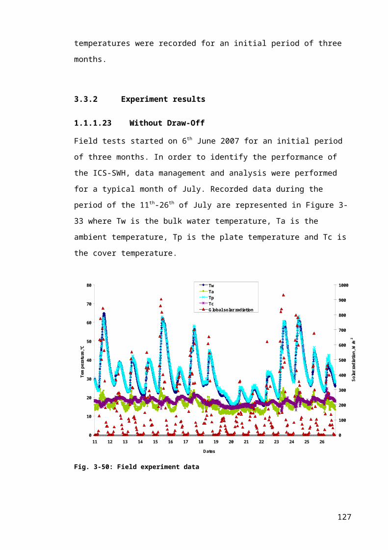
findings and the ability of the model to predict the water bulk temperature in the ICS-

SWH.

The laboratory macro-model was able to compare and predict the temperature variation

in diverse ICS-SWH configurations with different geometry, number of fins, internal

temperature and constant heat flux for a given aspect ratio.

4.1.9.2 Stratification model

The objective of this study was to model stratification profiles with time in an ICS-

SWH subjected to laboratory conditions. Three month full-scale experimental

laboratory tests were employed to validate the model.

The stratification profile changes with time and therefore needed to be modelled to

effectively predict the collector performance. Improvements to a previous laboratory

macro-model were incorporated. This allowed longitudinal stratification of temperature

within the solar collector to be determined based on the mean water temperature given

by the macro model, the given heat flux and the total time of exposure.

Computational results from the model were found to be in close agreement with the

experimental data with a tendency of the model to over-predict computed values by

nearly half of one degree Celsius at high heat fluxes. Results were validated by using

the model with wattages not used in the development phase of the program. Extreme

range simulations showed the suitability of the programme to display temperature

stratification.

4.1.9.3 Field model

Further work on the initial laboratory thermal model resulted in the development of a

thermal model suitable to predict bulk water temperature in real weather conditions.

Simulations for a 5 and 50 day period were undertaken. Both simulations showed that

computational results were found to be in close agreement with the experimental field

measurements. This statement was validated by statistical methods suggesting that the

field macro-model is a robust tool to compute bulk water temperature in the ICS-SWH

for any weather conditions.

137

This model was able to compare the temperature variation and predict the bulk water

temperature in diverse ICS-SWH configurations, with different geometry, number of

fins and external weather conditions for a given aspect ratio.

Although this model only gives mean values of water temperature, while in reality this

varies along the longitudinal height of the collector, it gives a good estimation of the

ICS-SWH performance. Results for the 50 day period also demonstrated that the

simulation can be extended which could result in a useful tool to estimate the yearly

performance of the ICS-SWH.

4.2 Micro model – CFD

A Computational Fluid Dynamic (CFD) study was undertaken to model flow and heat

transfer in the three-dimensional (3D) SWH geometry to provide useful information

about performance of the collector and evaluate design improvements. A first analysis

was undertaken for a four-fin collector designed as a mean of improving its

performance.

4.2.1 Purpose and fin optimisation

The CFD analysis of the ICS-SWH was undertaken in order to improve the four-fin

ICS-SWH performance by optimising the fin spacing. Prior to simulation, issues

regarding the parameters influencing fin optimisation need to be determined, constraints

stated, heat transfer parameters outlined, and the type of CFD analysis established.

Fin material, length, thickness, and the number of fins in the ICS-SWH are the four

main parameters to be defined when analysing fin optimisation. The material thermal

conductivity is an intrinsic parameter for an effective ICS-SWH. The low density, high

thermal conductivity and recyclable properties of aluminium highlighted the suitability

of this material as already discussed in section 3.1.1.

The fin length was fixed at a maximum of 800mm. Fins are used to increase the heat

transfer from the heated surface by increasing the effective surface area. The

effectiveness of the fin is enhanced by increasing the ratio of the perimeter to the cross-

sectional area ( ) as stated by Incropera and Dewitt (2001) therefore the use of thin,

but closely spaced fins is preferred, with the provision that the fin gap is not reduced to

a value where flow between the fins is severely impeded, thereby reducing the

138

convection coefficient. The study investigated the improvement in performance of the

ICS-SWH by increasing the number of fins.

Three main constraints were taken into consideration for design improvement and

included: cost, volume (50 litre tank size) and manufacturing ability.

Three main heat transfer parameters influence the ICS-SWH performance and can be

recapitulated as: the shape of fins, the angle of inclination of the heater, and time of

exposure to incident solar radiation. Due to manufacturing constraints, simple

rectangular shapes of fins were considered. A 45° inclination angle and a 300W/m2 heat

flux were taken as the reference conditions.

Finally, the type of CFD analysis, 2D or 3D, is an important parameter to consider. A

previous study of Muneer et al (2006a) outlined that 2D analysis was sufficient for a

satisfactory analysis of the system. However, 2D analysis would only suffice for a

horizontal inclination of the heater. For any angle above zero a gradient exists in the

longitudinal direction making a 2D analysis insufficient. Hence, based on a 45°

inclination of the collector, a 3D analysis was undertaken. As the quiescent fluid is

unavailable in CFD simulation, the process was assumed transient.

4.2.2 Capabilities and limitations

CFD in simple terms is the use of computer and numerical methods to solve and analyse

problems involving fluid flow. It is very often used in product concept, product

development and also virtual prototyping as it provides complementary information

about environmental performances and significantly reduces the amount of

experimental work needed. CFD-Fluent software, based on the finite volume method

offering a wide array of physical 2D and 3D models, was used for this study. Recent

studies indicate an increase in the use of CFD tools for analysing and optimising design

and performances of solar collector’s. This is despite some inaccurate predictions due to

the assumptions involved in modelling calculations stated by Groenhout et al (2002).

This model provided information about collector performance and was a useful tool for

design improvements providing detailed pictures of fluid movements and stratification

occurring in the collector.

Despite these advantages the CFD micro-model requires considerable skill to operate

thus requiring an extended training time and incurs high annual license and maintenance

costs. Regardless of an increased speed of computation available, CFD still cannot be

139

used for real time computation. Numerical analyses require considerable time to set up

and perform. Finally, software codes are locked which make them unavailable for

improvements

4.2.3 Model calibration

The modelling process was carried out for 3D analysis using CFD-Fluent 6.2 software.

Gambit 2.2 was used to mesh the model. The simple and regular geometry of the model

suggested the use of a quad structured mesh of size 1mm based on Henderson et al

(2007). Two different boundary condition types were applied on the absorber plate for

tests, depending on the purpose of the simulation. Optimisation simulations used a

constant heat flux of 300W/m2 as the boundary condition on the absorber plate. A

constant absorber plate temperature boundary condition was applied when comparing

the heat absorbed by the two ICS-SWH designs. According to these conditions the

program calculated the temperature field in the geometry and as a result values at the

nodes were displayed. Results are presented in section 4.2.4.

4.2.4 Modelling results

Stratification is essential for good performance of a solar collector and is significant

when trying to optimise the collector for draw-off as was observed in Chapter 3;

however, better mixing in the tank results in higher rates of heat transfer. Furthermore,

the addition of fins might give a differential of temperature – lower from the top to the

bottom of the ICS-SHW – but will optimise the transfer of energy into water. A CFD

stratification analysis was developed for the four-fin ICS-SWH design and then

undertaken for a second design using five fins to compare both water stratification and

velocity magnitude for a given time and heat transfer through time.

4.2.4.1 Fin heat transfer

A good understanding of the influence of extended surfaces is important when seeking

performance enhancement of the ICS-SWH. Figure 4-25 represents the temperature of

the fins after an elapsed time of 60 minutes and a simulated heat flux on the absorber

plate of 300 W/m2. Heat is transferred through the fins from the top of the collector to

the bottom where the water temperature is cooler. This results from gravity and

buoyancy effects. Water with different temperatures will settle at a height in the ICS-

SWH corresponding to the density of the fluid. Hot water of low density will naturally

settle in upper layers while cold water of high density will fall to the bottom layers.

During the first three hours of the charging process, high temperature stratification

140

occurs in the ICS-SWH. With time, temperatures in the upper layers become fully

established and reach an equilibrium causing the lower layer to increase in temperature

and therefore decrease the density gradient of water inside the ICS-SWH.

Fig. 4-85: Temperature stratification of fins and middle line of water collector

In order to ease the comprehension of the analysis process a discussion of the initial four-fin collector design is discussed below.

4.2.4.2 Four-fin collector design

The display of the water velocity profile was completed in Figure 4-26. Velocity was

observed to increase with the longitudinal length and then decrease as it gets closer to

the top of the collector. This can be explained by the accumulation of hot water at the

top of the collector reducing the velocity boundary layer and promoting diffusion of

heat with time. It is observed in Figure 4-26 that an increase, followed by a decrease,

pursued by an increase in velocity occurs between the fins. This decline in velocity

between the fins suggests that additional fins could be incorporated in the design to

increase the velocity magnitude.

141

Fig. 4-86: Velocity profile – 4 fins, top view, after 20 min

The horizontal plane view of velocity profile in Figure 4-27 supports this observation

and shows that high velocities occur at the absorber plate where higher temperatures are

experienced.

Fig. 4-87: Velocity profile – 4 fins, side view, after 20 min

142

Higher velocities

Higher

velocities

Results showed that the overall velocity increased with time until it reached a peak

value from which velocity magnitude declines with the passage of time. The increase is

due to a high heat flux through the fins to the water occurring after the initial

capacitance effect of the system. With time, hot water builds up at the top of the

collector as shown in Figure 4-28 resulting in a decline of heat transfer and therefore

heat is diffused from the system.

Fig. 4-88: Longitudinal water temperature stratification – 4 fins, front view, after 20min

Figures 4-28 and 4-29 represent the longitudinal temperature stratification in the

collector inclined at 45. As predicted, higher temperatures occur in the top of the

collector. Stratification occurs for a maximum water temperature of 295.9K at the top

of the collector to a minimum temperature of 293.3K at the bottom; a 2.6K

temperature gradient.

143

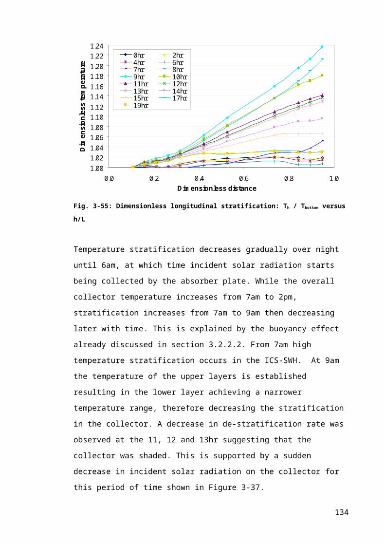
Fig. 4-89: Longitudinal water temperature stratification – 4 fins, side view, after 20min

In an attempt to improve the heat transfer one fin was added to the original ICS-SWH

design. New 3D velocity and stratification analysis were undertaken for the five-fin

ICS-SWH configuration.

4.2.4.3 Five-fin collector design

Figures 4-30 and 4-31 display the velocity profile of the new ICS-SWH. An increase in

velocity, compared to the four-fin design was observed resulting in an increase of 2% in

the maximum velocity. The main velocity pattern occurs between 1.90mm/s to 3.8mm/s

for the five-fin collector compared with a 1.86mm/s to 3.72mm/s for four-fin design.

144

Fig. 4-90: Velocity profile – 5 fins, top view, after 20 min

Fig. 4-91: Velocity profile – 5 fins, side view, after 20 min

The longitudinal temperature stratification of the five fin collector is shown in Figure 4-

32. Stratification occurs from a maximum water temperature of 295.9K at the top to a

145

minimum temperature of 293.8K at the bottom of the collector, resulting in a 2.1K

temperature difference. This corresponds to a 19% decrease in stratification.

Fig. 4-92: Longitudinal water temperature stratification - 5 fins, side view, after 20min

4.2.4.4 Improvements

Previous observation showed that the five-fin collector achieved an increase in velocity

of 2% compared to the four-fin design, while longitudinal water temperature

stratification decreased by 19%. This could be explained by the addition of the fins

responsible for an increased transfer of heat inside the collector, thus increasing velocity

and overall temperature in the collector.

In order to demonstrate that five fins is a more suitable geometry arrangement for

optimal collector design, a 3D CFD analysis was carried out assuming a constant

temperature boundary condition on the absorber plate set at 313K. The fluid departure

temperature was set at 293K. Despite the fact that the system is under a constant heat

flux, using a constant input temperature allowed the heat absorbed by both collectors to

be derived as shown in Figure 4-33.

146

294

296

298

300

302

304

306

308

310

312

314

0 10 20 30 40 50 60Time, mn

Ave

rage

d w

ater

tem

pera

ture

, °C

0

500

1000

1500

2000

2500

3000

3500

4000

4500

Wat

tage

tran

smitt

ed, W

/m2

4 fins - average Tw5 fins - average Tw4 fins - heat transmittance5 fins - heat transmittance

Fig. 4-93: Heat transfer and water temperature profiles in the ICS-SWH

Assuming a constant temperature boundary condition on the absorber plate resulted in

high rates of heat transmittance. This figure allows a comparison of the rate heat is

absorbed by both collectors. Initially, for the first ten minutes, more heat was absorbed

by the five-fin collector compared to the four-fin. This is linked to a frenzy of heat

transfer activity as the fins are surrounded by cooler water. After ten minutes the five

fins are surrounded with warmer water than the four fin design. The difference in

temperature between the four fins and the water is higher resulting in a higher heat flux.

Both profiles reach a peak value at the equilibrium temperature 313K set as the

boundary condition.

4.2.5 Discussion on CFD

This section reported the implementation of a four-fin ICS-SWH concept utilising CFD-

Fluent software through Gambit in order to optimise its design performance. Initial

results of the four-fin ICS-SWH indicated that one fin could be added to the original

design to improve the heat transfer. A 3D CFD simulation was then undertaken for a

five-fin ICS-SWH. Two boundary conditions were applied to the systems in order to

compare the water temperature stratification achieved and the heat transferred to the

water body by each collector.

The first boundary condition applied to the systems consisted of a constant heat flux on

the absorber plate. This method was used to characterise the temperature stratification

147

and the velocity magnitude within both collectors. Despite a minor decrease in

temperature gradient between the top to bottom in the five-fin ICS-SWH, it was clearly

observed that stratification remained. It is important to state that the addition of fins

should not impede the flow between the fins (as was experienced when trialling a multi-

fin design in an earlier study), thereby reducing the convection coefficient as stated by

Incropera and Dewitt (2001). Results showed that the addition of one fin in the collector

increased the velocity in the collector which has a corresponding increase on the Nusselt

number; raising the heat transfer coefficient in a predictable manner as stated by Ozoe

(1974a). The velocity magnitude was also observed to decrease with time for both

collectors with the water becoming warmer.

A second boundary condition applied to the systems consisted of a constant temperature

on the absorber plate which was used to characterise the heat absorbed by each

collector. Results revealed that the addition of one fin accounts for the increased transfer

of heat inside the collector. It was observed that the five fins supplied more energy to

the collector than four at the beginning of the charging process. The intermittent

availability of incident solar radiation in Scotland shows high potential for this type of

improvement as it is advantageous to have a rapid heating process.

In light of the results presented in this paper, the five-fin collector performed generally

better than the original four-fin collector. Therefore, this new design could be suggested

as a new arrangement of the collector assuming that the cost associated with this

improvement is negligible.

4.3 Concluding remarks

This chapter explored the modelling of ICS-SWH’s in order to assess their performance.

To start with, two macro-models for fluid flow and heat transfer were developed using

Visual Basic for Applications (VBA). Both generated corresponding bulk water

temperature’s in the collector with given hourly incident solar radiation (W/m2),

ambient temperature and inlet water temperature and therefore predictable ICS-SWH

performances. The first model was developed for laboratory conditions and modelled

bulk water temperature and stratification profiles over time in an ICS-SWH while the

second model predicted the bulk water temperature in the ICS-SWH for field weather

conditions.

Statistical methods and extreme range tests suggested that both models were robust and

could predict the performance of an ICS-SWH at any location and with different

148

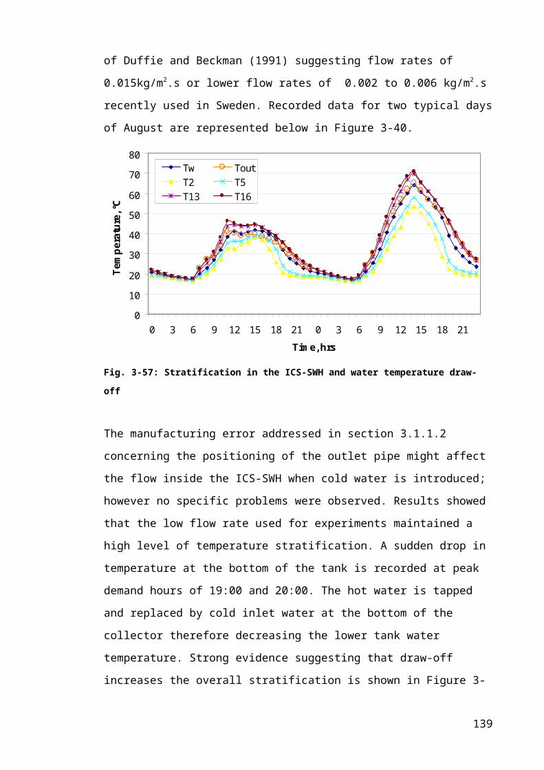
installation configurations. The field macro-model also demonstrated that a simulation

could be extended which could result in a useful tool to estimate the perennial

performance of the ICS-SWH. A life cycle assessment (LCA) based on this statement

was then carried out and is presented in Chapter 5. An account of uncertainties and

propagation of errors associated with modelling and the accuracy of statistical methods

used was addressed.

A CFD-Fluent analysis of the four-fin ICS-SWH concept was simulated in order to

optimise the design performance of the original concept and resulted in a new

simulation for a five-fin ICS-SWH. The new design showed high potential for Scottish

applications due to its rapid heating process which is advantageous in locations where

availability of incident solar radiation is intermittent. Therefore, this design could be

suggested as a new arrangement of the collector assuming that the cost associated with

this improvement is negligible.

In conclusion, this section of the thesis opens an avenue for future ICS-SWH design

optimisation but also widens the utilisation of the field macro-model developed by

showing its potential to provide data for a full year’s performance and therefore provide

an effective life cycle assessment of the ICS-SWH.

149

0

10

20

30

40

50

60

70

Time

Tem

pera

ture

, °C

Tw_ExperimentalTw_Computed

Fig. 4-94: Total data - measured and computed for a 50 day period: 7th June – 27th July 2007

150

CHAPTER 5 LIFE CYCLE ASSESSMENT (LCA)

Industries apply Life Cycle Assessment (LCA) as a technique to identify significant

environmental impacts of their products in order to improve their environmental

performance during their whole life cycle. This chapter performs a streamlined LCA of

different types of ICS-SWH designed for use in a Scottish environment. Firstly, the goal

and scope of the LCA were described. A material inventory providing general

information regarding material production processes used in the ICS-SWHs was

provided. An energy analysis of the ICS-SWHs using embodied energy of materials,

complemented by their associated environmental impacts were then dealt with. Finally,

a monetary analysis (MA) was provided enabling a cost comparison of the different

ICS-SWH alternatives identifying their value per pound Sterling spent.

5.1 Goal and Scope

The first step is to define the reference metric used in this study to quantify performance

of the ICS-SWH. International Organization for Standardization - ISO (2006)

demonstrates that a reference unit in any LCA needs to be determined in order to

compare collected data from different studies of the same product category. This study

is carried out to determine the best ICS-SWH alternative between three ICS-SWHs

presented for analysis. Based on the work of Ardente et al (2003), a reference unit (or

Functional Unit) equal to the entire equipment was used to benchmark this analysis.

The three ICS-SWHs systems assessed in this study correspond to two aluminium

construction of 1.5 and 3mm thickness (AL-1.5 and AL-3) and one of stainless-steel of

1.5mm (ST-1.5) incorporating extended heat transfer surfaces. Each ICS-SWH is

composed of three main components identified below and shown in Figure 5-1:

1. The collector (including the absorber plate and the water tank)

2. The glass wool insulation

3. The glass cover

4. The wooden box

151

Fig. 5-95: Sectional view of the aluminium ICS SWH. Note: a dimension drawing is shown in

Figure 3-1

The collector was categorised as a passive ICS-SWH. The water tank and absorber plate

are integrated into one unit. This type of collector is recommended for medium to low

temperature domestic water heating applications. The ICS-SWHs were assumed to be

directly installed on sloping roofs of 45 angle of inclination. Impacts associated with

each collector component were analysed in order to identify the main life cycle issues

affecting each component of the ICS-SWHs.

The LCA of each ICS-SWH type will provide an analysis of the environmental benefit

of operating these heaters in Scottish weather conditions in order to appreciate if this

tool can identify a best ICS-SWHs alternative. A material inventory introducing the

main component production processes was first carried out to understand their potential

harms to the environment and their energy requirements during production. An energy

and environmental impact analysis for each component was then performed.

Interpretation of results by introducing energy savings and carbon emission reduction

followed by a monetary saving analysis were determined. Assumptions for the analysis

included a typical water inlet temperature of 12C for Scotland and a domestic hot water

(DHW) demand temperature of 55C, assuming a daily draw-off regime of water at

4pm. On days of poor insolation either electric or hydrocarbon back-up sources elevate

the water temperature to 55°C, this is accounted in the LCA and cost analysis. The DTI

(2002) stated that the average population of a UK home is approximately three people,

with each consuming 50 litres of hot water per day as identified in a later survey carried

on behalf of DTI (2005) and DEFRA. Given that the capacity of the ICS-SWHs is 50

litres with 1m2 of collector plate, all interpretations were based on the installation of 3m2

of collector plate or 150 litres to meet typical domestic demand from an installation.

5.2 Material inventory

The following section discusses the processes involved in production of the main

materials used in the construction of the ICS-SWHs.

Glass Cover

Glass wool insulation Collector

Wooden box

152

5.2.1 Stainless-steel

There are a number of stages involved in producing stainless-steel for commercial use.

Stainless-steel is produced from ore and scrap metal. The principal ore used is hematite

which contains almost 70% iron. Scrap iron and stainless-steel and various alloys of

chromium (and nickel, molybdenum etc. depending on the stainless type) are used in

stainless-steel making today. The main process used at present for refining stainless-

steel is the electric arc furnace used to produce carbon and alloy steels. A current is

passed through an electrode resulting in a temperature increase to a point where the

scrap and alloys melt. The molten material is then transferred into an Argon Oxygen

Decarbonisation container, where the carbon levels are reduced and the final alloy

additions are made to make the composition chemistry depending on the type of

stainless-steel.

Stainless-steels are a group of high alloy steels that are designed to provide high

corrosion resistance. This is provided by the thin oxide film which forms due to the

chromium element in the stainless-steel reacting with oxygen in the atmosphere. The

stainless-steel 304 used in this study is classified as an austenitic steel with an alloy

containing 18-20% of chromium and 8-10% of nickel resulting in a very ductile

material and a good corrosion resistance as stated by Groover (2006).

5.2.2 Aluminium

In a similar fashion, aluminium is produced from ore (Bauxite) and scrap metal. Bauxite

is mined and refined in order to extract aluminium for use. The ore is first washed and

crushed into a fine powder. The aluminium is then extracted from the bauxite as

aluminium oxide (alumina) which is subsequently broken down and separated into

aluminium and oxygen gas using an electrolysis process also called smelting. The

aluminium is then alloyed with other materials and is then processed through casting,

rolling or extrusion for further fabrication of aluminium products.

Aluminium is one of the newer materials among the principal metals on the market. Its

low density made it an attractive choice use in engineering. Aluminium also has high

electrical and thermal conductivity and an excellent corrosion resistance due to the thin

layer of aluminium oxide that forms on its surface when exposed to oxygen. It is a very

ductile material and although it is known to be relatively low in strength it can be

alloyed and heat treated to allow it to compete with steels.

153

5.2.3 Glass wool insulation

Glass-wool is produced from raw materials such as sand, recycled glass, soda ash,

limestone and glass-wool scrap from the production process. Reusing of waste off-cuts

into the production process reduces raw material input and therefore energy

requirements.

Recycled glass from building windows, car glass and bottle glass is increasingly used in

the manufacturing of glass wool accounting for 30% to 60% of the raw material input.

The raw material mix is then melted at high temperature ranging from 1300°C to

1500°C in an electric or gas furnace while fumes and dusts are cleaned by filters to

minimise environmental impact.

The melted glass is then converted into fibres with its passage through a spinner drilled

with holes and through a fibre attenuation using high temperature gas jet streams. Small

quantities of binding agents are then added to the fibres in order to give the desired

structure and density required for its end-use application. The glass wool mat finally

goes to a curing oven heated at around 200°C where it gets its final shape, strength and

stability, and where it is laminated and polymerised. The glass wool is then cut in width

and length at the required dimensions according to its final usage. The product is then

tightly compressed in order to reduce the product volume in the packaging resulting in

an easier and cheaper storage and transport of the product. Figure 5-2 represents the

glass wool production process illustrated by the European Insulation Manufacturers

Association - ERIMA (2007).

154

Fig. 5-96: Glass wool production process, Source: ERIMA (2007)

5.2.4 Window glass

The window glass is produced using the float glass method. Raw materials such as soda

lime glass which principally contains silica sand, soda ash and limestone are mixed and

weighed and then flow into a furnace heated to 1500°C. Melting, refining and

homogenising take place simultaneously in the furnace and determine the glass quality.

Compositions of the glass can be modified during this process to change the properties

of the finished product such as adding magnesia to help reduce devitrification as stated

by Groover (2006).

The molten glass is then fed onto a float bath where it is floated on top of a bath of

molten tin in a continuous ribbon and starts to cool slowly. The ribbon then goes

through a coating stage through chemical vapour deposition laying down a variety of

coatings to vary the optical properties of float glass depending on the final application.

The ribbon then passes through an annealing process where glass is slowly cooled in a

Lehr oven to prevent build up of stress. The glass is cooled under controlled conditions

155

until it reaches room temperature and is then cut to the desired shape and size. Figure 5-

3 represents the window glass production process illustrated by Made How (2007).

Fig. 5-97: Window glasss production process, Source: Made How (2007)

5.2.5 Timber

The timber frame was produced from UK grown mixed conifer logs through a sawmill

process. In the first stage the grading process pre-sorts conifer logs into size and end

use, before input to the sawmill. The logs then go through a debarker prior to sawing to

remove bark from logs. The bark waste is then reused as raw material for horticulture.

Subsequently debarked logs go through the sawmill to produce dimensional lumber.

The cut products are then sorted through infra-red scanning equipment ensuring that

only product of the required grade is included in the finished pack. The timber is then

cut to the desired lengths by multiple cross cut machinery for the packaging process.

Finally, preservative treatment is applied to timber products to ensure long term

protection and service life of the timber.

5.3 Energy analysis

The energy analysis concerns energy flows occurring during the life cycle of the

product. The energy consumption can be split in two phases: Direct energy and

Embodied energy. Direct energy corresponds to the energy used during a life cycle step

including electricity or heat energy employed during the production of the collector or

156

fuel for transport. Embodied energy corresponds to the energy consumed by all the

processes associated with the production of the individual materials employed.

The total energy consumption is obtained by summing embodied and direct energy

contributions. However, Ardente et al (2005a) showed that direct energy consumption

only account for 10% of the overall energy consumption. Therefore, the streamlined

LCA only accounts for embodied energy involved in the production processes of the

ICS-SWHs materials.

Embodied energy assesses the total primary energy consumed over the whole life time

of a product with the boundaries ideally being set from the extraction of raw materials

to the end of the product’s lifetime; a boundary condition which is known as “cradle to

grave”. Data regarding the embodied energy of materials refers to the Inventory of

Carbon and Energy report issued by Hammond and Jones (2006). Embodied energy of

each material presented in Table 5-1 is based on average UK market data.

Table 5-13: Embodied energy of materials

Material Embodied energy (MJ/kg)

Stainless-steel 51.5

Aluminium 150.2

Glass 13.5

Timber 8.7

Glass wool 28.0

The aluminium embodied energy production was found to be 150.2 MJ/kg

corresponding to an average of 33% recycled and 67% raw aluminium material. Future

scenarios could be imagined of 85% recycled and 15% raw aluminium material which

would reduce the embodied energy of aluminium production process to 53.7J/kg.

A breakdown of the materials used to produce the final ICS-SWHs was quantified in

order to calculate their respective overall embodied energy. Table 5-2 reports the mass

balance of a 1m2 collector summarising the quantity of materials required for each ICS-

SWH.

157

Table 5-14: Mass balance of the collectors

Collector type Material Mass (kg)

Stainless-steel Stainless-steel (1.5mm sheet) 28.0

1.5mm Glass 12.6

Timber 30.7

Glass wool 3.5

Aluminium Aluminium (1.5mm sheet) 9.8

1.5mm Glass 12.6

Timber 30.7

Glass wool 3.5

Aluminium Aluminium (3mm sheet) 19.6

3mm Glass 12.6

Timber 30.7

Glass wool 3.5

The embodied energy and effect on the energy balance of materials involved in the

construction of the ICS-SWHs were then calculated; hence the overall embodied energy

of the ICS-SWHs was determined. Table 5-3 provides information gathered on each

ICS-SWH.

Table 5-15: Embodied energy and incidence of materials on the energy balance

Collector type Material Embodied energy (MJ) Incidence (%)

Stainless-steel Stainless-steel (1.5mm sheet) 1442.0 73.01.5mm Timber 265.7 13.5

Glass 169.7 8.6Glass wool 97.2 4.9

  Total 1974.6 100.0

Aluminium Aluminium (1.5mm sheet) 1472.0 73.41.5mm Timber 265.7 13.3

Glass 169.7 8.5Glass wool 97.2 4.8

  Total 2004.6 100.0

Aluminium Aluminium (3mm sheet) 2943.9 84.73mm Timber 265.7 7.6

Glass 169.7 4.9Glass wool 97.2 2.8

  Total 3476.5 100.0

Based on the earlier discussed DTI (2002) study in section 5.1, results have to be

translated to 3m2 of collector plate or 150 litres, to reproduce an appropriate study for

158

UK homes. Primary energy consumption, measured in kWh, for the production of 3m2

ICS-SWHs during the complete life cycle phase, , is represented in Table 5-4.

Table 5-16: Energy analysis for a 3m2 installation

Collector type Material Embodied energy (kWh)

Stainless-steel 1.5mm

Stainless-steel (1.5mm sheet) 1645.5

Aluminium1.5mm

Aluminium (1.5mm sheet) 1670.4

Aluminium3mm

Aluminium (3mm sheet) 2897.1

The energy analysis provided the total energy and material consumption for the

production of each ICS-SWH. This analysis enables the evaluation of comparative

environmental impacts and potential improvements which are provided in the following

sections.

5.4 Environmental impacts

This section aims to provide an understanding and evaluation of the magnitude and

significance of the potential environmental impacts of each ICS-SWH. Resource

consumption, air emissions, water emissions, waste and solid pollutants are the main

environmental impacts. However, the streamlined LCA only accounted for the

environmental impact of air emissions in order to ease the system analysis.

This environmental impact can be classified as either a direct or indirect emission.

Based on Ardente et al’s (2005a) study, direct emissions were neglected as they

generally represent an overall incidence of 10%. Therefore, only indirect emissions

were considered. Indirect emissions are mainly related to the raw materials production

process.

Based on the IPCC (2007) report, increased industrial activity and other human

activities have increased CO2 concentrations in the atmosphere. CO2 being a greenhouse

gas, this could result in an increase in mean global temperature. Based on this statement

CO2 was chosen as the indicator of this category and embodied CO2 associated with the

raw material production process of each ICS-SWHs was determined. Embodied CO2

refers to the amount of carbon dioxide emissions that result from the processes required

159

to produce the finished product. Data regarding the embodied carbon of materials refers

to the Inventory of Carbon and Energy report issued by Hammond and Jones (2006).

Embodied CO2 emissions of each material are presented in Table 5-4 and refer to UK

average market data.

Table 5-17: Embodied carbon dioxide of materials

Material Embodied CO2 (kgCO2/kg)

Stainless-steel 6.2

Virgin aluminium 8.4

Glass 0.8

Timber 0.5

Glass wool 1.4

The embodied carbon UK average data of aluminium production was found to be 8.35

kgCO2/kg. Future scenarios having 85% recycled and 15% raw aluminium material

would bring the embodied carbon down to 3.17 kgCO2/kg.

Based on the figures from Table 5-2 the embodied carbon and effect on the energy

balance of materials involved in construction of the ICS-SWHs was then calculated;

hence the overall embodied carbon of the ICS-SWHs was determined. Table 5-5

provides information gathered on each collector.

Table 5-18: Embodied energy and impacts of materials on the energy balance

Collector type Material Embodied CO2 (kgCO2) Impacts (%)

Stainless-steel Stainless-steel 172.2 85.61.5mm Timber 14.6 7.3

Glass 9.7 4.8Glass wool 4.7 2.3

  Total 201.2 100Aluminium Aluminium 81.8 73.81.5mm Timber 14.6 13.2

Glass 9.7 8.8Glass wool 4.7 4.2

  Total 110.8 100Aluminium Aluminium 163.7 85.03mm Timber 14.6 7.6

Glass 9.7 5.0Glass wool 4.7 2.4

  Total 192.7 100

160

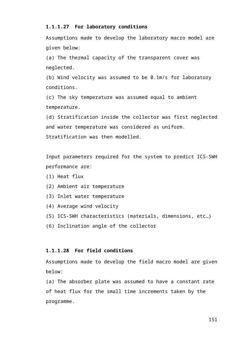
Based on the DTI (2002) study the environmental impacts were considered for 3m2 of

collector plate or 150 litres. Total CO2 emissions, , related to the production of

3m2 ICS-SWHs are represented in Table 5-7.

Table 5-19: Total CO2 emissions for a 3m2 installation

Collector type Material Embodied CO2 (kgCO2)

Stainless-steel1.5mm

Stainless-steel (1.5mm sheet) 603.6

Aluminium1.5mm

Aluminium (1.5mm sheet) 332.4

Aluminium3mm

Aluminium (3mm sheet) 577.9

5.5 Interpretation

5.5.1 Identification of Energy and Environmental issues

An analysis of the energy and environmental impacts developed in sections 5.3 and 5.4

was performed in order to identify and evaluate the significant issues based on the

above results. It is a valuable step in order to compare the different production

alternatives and which material input has the most impact on ICS-SWH construction.

5.5.1.1 Energy issues

The embodied energy related to the collector production depends on the material type

and mass and is the main contributor to the ICS-SWHs overall embodied energy. The

embodied energy associated with each material depends on the quantity needed and the

energy intensity of the material’s production.

Although the embodied energy per kilogram of aluminium is 66% higher than stainless-

steel, the overall embodied energy of the collector, for an identical material thickness, is

of the same magnitude as shown in Table 5-3. This is explained by the 65% lower

aluminium density of 2770kg/m3 compared with 7900kg/m3 for stainless-steel.

It was also observed from Table 5-1 and 5-3 that from the three remaining materials

(glass, timber and glass-wool), glass wool has the highest embodied energy per

kilogram but has the smallest effect on the overall ICS-SWH embodied energy due to

its low mass. Vice versa the overall embodied energy of timber was found much higher

than glass-wool. This is explained by the timber mass being nine times that of glass-161

wool. Similar observations were made for the glass compared with timber and glass-

wool materials.

5.5.1.2 Environmental issues

The embodied carbon emissions associated with each material depends on the CO2

released during their production; depending essentially on the type of fossil fuels used

and the amount of material needed.

Although the embodied carbon emissions per kilogram of aluminium are 26% higher

than the stainless-steel; as shown in Table 5-5, the overall embodied carbon emissions

of each collector, for an identical material thickness, is 45% lower by using aluminium

as shown in Table 5-6. It was also noted that even by doubling the thickness of the

aluminium (AL-3), the embodied carbon emissions are still 4% lower than the ST-1.5.

This can be explained by the recyclable property of aluminium. This verifies the

statement made in the above section 5.5.1.1, showing that despite the higher embodied

carbon emissions per kilogram of aluminium, the lower mass of aluminium needed to

produce an identical collector resulted in lower overall embodied carbon emissions.

Each material was then weighed to calculate their contribution to the overall carbon

emissions of each ICS-SWH. Again, it was observed from Table 5-5 and 5-6 that from

the three remaining materials (glass, timber and glass-wool), glass wool had the highest

embodied carbon emissions per kilogram but resulted in the smallest effect on the

overall ICS-SWH embodied carbon emissions due to its low mass. Vice versa timber

had the lowest embodied carbon emissions per kilogram despite having the biggest

effect on the overall ICS-SWH embodied carbon emissions due to its higher mass.

5.5.2 ICS-SWHs energy and carbon dioxide savings

A cost-benefit analysis of the energy and environmental parameters of each ICS-SWH

was performed in this section. For this analysis the useful energy saved annually, ,

and CO2 emission savings, , need to be determined.

5.5.2.1 System output

The macro-model developed in Chapter 4 for field weather conditions was used to

generate corresponding bulk water temperature in the collector for each ICS-SWH. Data

regarding the hourly solar radiation and other climatic parameters necessary for the 162

simulation come from the European Commission Joint Research Centre, Institute for

Environment and Sustainability (IES) (2007) for Edinburgh location. The daily,

monthly and annual energy savings and CO2 emission savings were then determined

assuming a typical inlet water temperature of 12C for Scotland and a required

temperature of 55C supposing a draw-off of water at 4pm daily.

The daily potential energy outputs from using the ICS-SWHs were calculated using

equation 5.1.

(5.1)

Where is the inlet/outlet temperature difference of the water (C)

is the assumed inlet temperature of the water of 12C (C)

is the modelled output water temperature at 4pm (C)

is the daily water flow rate assumed at 150l/day for 3m2 collector area

is the specific heat capacity of the water (J/kg.C)

The variation of the specific heat capacity of water over this temperature range is

negligible with a maximum variation of about 0.4% and was therefore assumed constant

at 4.2kJ/kg.C.

Monthly and useful energy saved annually, , were then calculated for each ICS-

SWH. Figure 5-4 presents useful energy saved annually by each ICS-SWH. This figure

was based on a 3m2 collector area installation heating 150 litres of water per day from a

starting temperature of 12°C to the required temperature of 55°C in Edinburgh weather

conditions.

163

1109

1107

1041

0 200 400 600 800 1000 1200

E s, kWh

Aluminiumcollector - 3mm

Aluminiumcollector - 1.5mm

Stainless-steelcollector - 1.5mm

Fig. 5-98: Useful energy saved annually for each ICS-SWH

The annual energy saving from using AL-3, AL-1.5 and ST-1.5 ICS-SWHs were found

to be 1109kWh, 1107kWh, 1041kWh respectively. Based on the previous assumption,

2747kWh is annually required to raise the daily 150 litres of water from 12°C to 55°C.

The ICS-SWHs did not raise the water by the required amount but partially fulfil the

daily domestic hot water needs. AL-3, AL-1.5 and ST-1.5 ICS-SWHs could save up to

40.4%, 40.3% and 37.9% of the required energy. Using a more conductive material

resulted in a 2.4% annual increase of energy savings while increasing the material

thickness resulted in only 0.1% annual increase.

A detailed picture of the monthly energy coverage (EC) of each ICS-SWH is provided

in Figure 5-5. The energy coverage represents the percentage ratio of the energy saved

and energy required to raise the 150 litres of water from 12°C to 55°C.

164

0

10

20

30

40

50

60

70

80

Jan Feb Mar Apr May Jun Jul Aug Sep Oct Nov Dec

Month

Sola

r fra

ctio

n, %

Aluminium collector - 3mmAluminium collector - 1.5mmStaniless-steel collector -1.5mm

Fig. 5-99: Solar fraction of AL-3, AL-1.5 and ST-1.5. Note: solar fraction is the amount of energy

provided by the ICS-SWH divided by the energy required to raise water temperature to 55oC

For each month it is evident that the ST-1.5 is under-performing compared with

aluminium ICS-SWHs. The AL-1.5 is slightly out-performed by the AL-3 ICS-SWH,

however AL-1.5 uses half the amount of material therefore suggesting AL-1.5 as the

best alternative. Each annual energy saving has an associated annual CO2 emission

saving presented in the next section.

5.5.2.2 CO2 savings

Domestic water heating is primarily accomplished using natural gas or electricity with

natural gas accounting for 60% of the UK water heating systems. In order to quantify

the annual CO2 emission savings, , detailed fuel conversion factors were

introduced. Such factors provide CO2 emissions expressed per unit activity such as fuel

or electricity consumed or distance travelled. Electricity and natural gas conversion

factors represents the fuel mix used for electricity generation, quality of coal consumed,

composition of the vehicle fleet and journey taken in that year. Based on data from the

UK inventory of Greenhouse Gas emissions produced for Department for Environment,

Food and Rural Affairs – DEFRA (2005), electricity and natural gas conversion factors

were taken as 0.43kgCO2/kWh and 0.19kgCO2/kWh respectively. The annual CO2

emission savings of each ICS-SWHs were then calculated depending on the fuel used in

the household and are presented in Figure 5-6.

165

211 210198

477 476448

0

50

100

150

200

250

300

350

400

450

500

Electricity Gas

Fuel

Ann

ual C

O 2 s

avin

gs, k

g

Aluminium collector - 3mmAluminium collector - 1.5mmStainless-steel collector - 1.5mm

Fig. 5-100: Annual CO2 savings by fuel type using ICS-SWHs

Depending on the type of ICS-SWH installed there is a potential for saving of 198-211

kgCO2 per year if assisting a gas water heating system. While this may seem an

insignificant figure in terms of the overall targets set under the Kyoto protocol, if half of

the 25 million homes in the UK had an ICS-SWH system installed to assist their daily

hot water needs, around 2.6 MtCO2 per year could be saved.

These results show that installation of ICS-SWHs in UK homes can contribute to

significant carbon dioxide reduction. In order to determine which of the three ICS-

SWHs would be the most viable solution, an energy payback time (EPBT) and carbon

dioxide emission payback time (ECPBT) were carried out in the next sections.

5.5.3 Energy payback time – EPBT

The energy payback time (EPBT) is defined by Ardente et al (2005b) as the time

necessary for an ICS-SWH to collect the energy equivalent to that used to produce it.

Therefore the EPBT can be expressed in equation 5.2.

166

(5.2)

Where is the energy input during the ICS-SWH life cycle (kWh), is the annual

useful energy saved by using the ICS-SWH (kWh/year) and is the annual energy

employed during the use of the ICS-SWH (kWh/year).

The use of a passive collector system or a solar driven pump was therefore assumed for

to be null. Hence EPBT were calculated for AL-3, AL-1.5 and ST-1.5. Results are

presented in Table 5-8.

Table 5-20: EPBT

Collector type (kWh) (kWh/year) EPBT (years)

ST-1.5 1646 1041 1.6AL-1.5 1670 1107 1.5AL-3 2897 1109 2.6

The energy payback times related to the studied ICS-SWHs were found to be lower than

three years. This value shows the great energy potential of such technology. A common

thought would be that the aluminium payback period should be significantly longer

because of its more intensive production process resulting in embodied energy value per

kilogram of material being three times the stainless-steel one. However, the recycling

property of aluminium decreases its embodied energy, bringing down the energy

payback time considerably. Future scenario of 85% recycled and 15% raw aluminium

material would lower the embodied energy of aluminium production therefore reducing

the EPBT of AL-1.5 to 10 months.

5.5.4 Carbon dioxide emission payback time – ECPBT

The ECPBT was calculated based on the previously calculated annual emission savings

of CO2, , in section 5.5.2.2. The ECPBT can be defined as the time necessary for an

ICS-SWH to equal the CO2 emissions released during the production and use of the

installation itself as stated by Ardente et al (2005b). It summarises the total impacts

during the life cycle and the emission savings. The ECPBT is expressed in equation 5.3.

167

(5.3)

Where is the total CO2 emissions related to the production of a 3m2 ICS-SWH

during its life cycle (kgCO2) represented in Table 5-7, is the annual CO2 emission

saving (kgCO2/year) represented in Figure 5-6 and is the annual CO2 emissions

related to the ICS-SWH use (kgCO2/year). represents the emissions saved by using

the ICS-SWH compared to the auxiliary system used in the household to deliver hot

water and therefore depends on the type of auxiliary heater employed.

The use of a passive collector system or a solar driven pump was assumed therefore

was set to null. ECPBT for AL-3, AL-1.5 and ST-1.5 were calculated and results

are presented in Table 5-9 and Figure 5-7.

Table 5-21: ECPBT

Collector type (kgCO2) (kgCO2/year) ECPBT (years)

Gas Electricity Gas ElectricityST-1.5 604 198 448 3.1 1.3AL-1.5 332 210 476 1.6 0.7AL-3 578 211 477 2.7 1.2

1.2

0.7

1.3

2.7

1.6

3.1

0.0

0.5

1.0

1.5

2.0

2.5

3.0

3.5

Gas Electricity

Fuel

ECPB

T, y

ears

Aluminium collector - 3mmAluminium collector - 1.5mmStainless-steel collector - 1.5mm

Fig. 5-101: ICS-SWH ECPBT: Categorisation with respect to fuel type

168

The carbon dioxide payback period depends on the auxiliary system used by the

household. Like the energy payback-time, the CO2 payback-time results were generally

lower than three years.

The per unit CO2 evolution of electricity is much higher than natural gas resulting in

shorter environmental payback period for households using electricity as an auxiliary

heating system. This is due to electricity having a high environmental impact due to the

fuel mix used in its generation. ECPBT ranges from 1.6, 2.7 to 3.1 years for the AL-1.5,

AL-3 to ST-1.5 respectively using gas while using electricity would result in a decrease

of ECPBT to 8 months, 1.2 and 1.3 years respectively; corresponding to a 56%

difference in ECPBT depending on the fuel type.

A considerable variation in the payback time of collectors of identical dimensions, Al-

1.5 and ST-1.5, was observed. This is explained by the recyclable property of

aluminium diminishing its embodied carbon and by its higher thermal conductivity

resulting in higher energy gain. A payback period based on future scenarios of 85%

recycled and 15% raw aluminium material would result in lowering the ECPBT to 10

and 5 months when gas and electricity auxiliary heating systems are used.

5.5.5 Conclusions and recommendations

An LCA was carried out for each ICS-SWH type in order to establish the ICS-SWH

with the smallest carbon footprint. It was found that despite the high amount of energy

to produce aluminium, the “light” and recyclable properties of the material resulted in

similar embodied energy when compared with stainless-steel. This resulted in a smaller

environmental impact due to lower carbon emissions released to the atmosphere during

the production process.

Energy and carbon dioxide savings associated by using those ICS-SWHs were modelled

and showed that although the AL-1.5 ICS-SWH was out-performed by 0.1% by the AL-

3 ICS-SWH, the fact that it only uses half the amount of material in producion makes it

more viable. The carbon dioxide savings showed that depending on the ICS-SWH

installed there is a potential for saving 6% more kgCO2 per year by using an Al-1.5

compare with a ST-1.5 and only 0.5% by increasing the thickness of a same ICS-SWH

material.

169

The EPBT of the ICS-SWHs was found to be consistently lower than three years for all

ICS-SWHs with the lowest EPBT value of 1 year 7 months achieved by the AL-1.5

ICS-SWH. This value shows the great energy potential of such a ICS-SWH design. The

calculations of the carbon dioxide emission payback times confirm the higher potential

of using an AL-1.5 ICS-SWH by decreasing the ECPBT by 42% and 48% when

compared with AL-3 and ST-1.5 ICS-SWHs respectively.

All results point to the AL-1.5 ICS-SWH as the best alternative to operate in Scottish

weather conditions. It would therefore be recommended to use an AL-1.5 ICS-SWH for

further investigations due to its energy and environmental benefits. Increasing the

recyclable percentage in the AL-1.5 could significantly reduce the environmental

impact of the collector. Copper and brass could be realistic alternatives to use in the

manufacture of the ICS-SWH in terms of embodied energy, malleability and thermal

conductivity. However, the cost of these materials being so much higher than that of

stainless-steel or aluminium would not make them economically viable. Economics

plays a central role in any decision to purchase a solar water heater system. The

customer is unlikely to buy an ICS-SWH if they know that its only benefits are to the

environment. Therefore, a monetary analysis was developed to consider the economics

of each system to ensure that such ICS-SWHs will be profitable.

5.6 Monetary analysis (MA)

The monetary analysis (MA) can be defined as an economic evaluation technique to

determine the total cost of owning and operating a product with time. The value of a

MA lies in the ability to compare the cost of product alternatives and to determine

which one provides the best value per Sterling pound spent. In order to achieve an

appropriate MA, an insight of the collector material costs is provided, followed by the

actual cost of the ICS-SWHs and a monetary payback time (MPBT) assessment.

5.6.1 Collector material costs

It is difficult to find a definite figure for the price of aluminium and stainless-steel as

they commonly fluctuate. Average figures obtained for the last year from May 2007 to

May 2008 would be £2900 per tonne of stainless-steel and £1445 per tonne of

aluminium. The large price difference can have several possible explanations. The main

factor of the cost difference between the two metals is the added cost of machining

stainless-steel compared with aluminium; which is ductile and more easily machined. 170

Wholesale metal suppliers MEPS and LME could guarantee costs up to three to four

months but not further than that period which reflects the frequency with which prices

vary. A comparison of the price trend of aluminium and stainless-steel over the last

three years is shown in Figure 5-8.

1000

2000

3000

4000

5000

6000

Mar

-05

Jun-

05

Sep

-05

Dec

-05

Mar

-06

Jun-

06

Sep

-06

Dec

-06

Mar

-07

Jun-

07

Sep

-07

Dec

-07

Mar

-08

Date

Alu

min

ium

Pric

e, $

US/

tonn

e Aluminium Stainless-steel

Fig. 5-102: Cost comparison

Stainless-steel has been the more expensive of the two materials but both materials have

been increasing at the same rate until recently. Over the course of the last three years the

price of stainless-steel has risen beyond levels that anyone inside or outside the

stainless-steel industry could have forecasted. There are a number of contributing

factors that have lead to these increased costs.

1 - Chinese stainless-steel consumption

There has been a recent and important increase in Chinese consumption of stainless-

steel which has caused a global price increase in spite of a consistent consumption for

the rest of the world. China has experienced phenomenal growth in the last five years

resulting in being the world’s largest stainless-steel consumer and has not yet reached

its peak.

2 - Raw material shortage

171

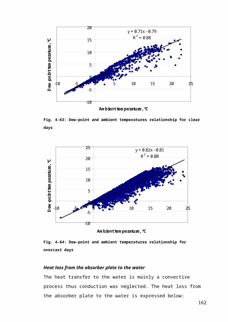
Scrap metal comes from waste stainless-steel items. Moll (2006) announced a decline

from 34.8% in 2004 to 32% by 2010 of the worldwide share of scrap in stainless-steel

production suggesting that scrap is being consumed at a far greater rate than it is being

created. This current scrap shortage results in a notable increase in scrap prices. Iron ore

is another material which is currently in short supply due to the significant lack of

investment in iron ore mines anywhere in the world except for China and South

America. Another main reason is the shortage of nickel ore supply, a major raw material

for stainless-steel production resulting in a high nickel price. These raw material

shortages result in rising stainless-steel production costs.

2 - Stainless-steel production

According to the International Stainless-steel Forum - ISSF (2007) global stainless-steel

production decreased by 2.9% in 2007. This happened across most regions and

countries except for China and the Asian region accounting for 60% of the world's

stainless-steel production. A strong increase in stainless-steel production occurred in the

first half of 2007 followed by a collapsed in the second half of the year after nickel

prices dropped resulting in stainless-steel being withdrawn from the first half of 2007

stocks.

3 - Shipping

Another item influencing stainless-steel prices is a shortage of shipping capacity. One of

the factors behind the growth in international trade over the past decade is a reduced

shipping cost but now the trade has grown to such an extent that there is a shortage of

shipping available. The higher cost of shipping is hampering the movement of raw

materials around the globe.

4 - Energy costs

Energy costs are another factor increasing stainless-steel production costs. Production

cost increases due to higher energy input costs (i.e. Electricity is an output from many

energy resources and is used to power most equipment and facilities). Energy markets

are experiencing high demand and limited supplies, resulting in volatile market and high

prices. Since energy is a key input in the production process, sharp increases per unit in

goods occur as stated by Velazquez (2006). Stainless-steel being an energy intensive

process uses significant energy input for their production resulting in higher costs.

172

5.6.2 ICS-SWHs costs

The price of installing a domestic flat plate collector solar water heating system in

the UK today is anywhere from £2,000 to £3,000 which would include delivery,

installation and associated equipments costs as stated by EST (2007). The majority of

solar water heating systems installed would come with a 5 to10 year warranty and

require very little maintenance. The costs of the materials used in the ICS-SWHs

investigated for this project are detailed in Table 5-10. Prices were updated to most

recent material cost data collected in May 2008.

Table 5-22: Raw material costs per square meter of collector

Collector type Collector cost (£) Material cost (£) ICS-SWH cost (£)

Stainless-steel1.5mm

352 105 457

Aluminium1.5mm

81 105 186

Aluminium3mm

161 105 266

The difference in price of the two materials is a reflection of the recent surge in

global stainless-steel prices. Aluminium prices were taken from London Metal

Exchange (LME) while stainless-steel 304b prices were taken from MEPS International

Ltd. While the cost of materials may not be very high, the additional labour and

delivery costs, along with other required parts such as a pump, controller, valves and

piping would raise the price of parts up to the region of £1,000.

To encourage the public to become involved in the effort to reduce carbon emissions,

government grants for homes that install these heating systems are made available. The

UK government Low Carbon Buildings Programme (LCBP) offers a £400 grant for

every professionally installed solar water heating system as stated by the DTI (2007).

Another grant available in Scotland from the Scottish Community Householder

Renewables Initiative (SCHRI) provides 30% of the installed cost up to a value of

£4,000 as stated by the Energy Saving Trusts (2007).

173

5.6.3 Monetary payback time (MPBT) analysis

The monetary payback time (MPBT) can be defined as the time necessary for the ICS-

SWH to achieve the monetary equivalent to its capital cost and is expressed in equation

5.4.

(5.4)

is the capital cost associated with the ICS-SWH life cycle (£), is the annual

monetary saved by using the ICS-SWH (£/year) and is the annual associated cost

of using ICS-SWHs such as operational and maintenance costs (£/year).

Gull Industries (2008) also suggested that ICS-SWHs are virtually maintenance free

although the glazing needs to be cleaned and the unit to be drained once a year, as is

recommended for auxiliary water heaters. It was then assumed for this study that annual

associated costs could be neglected, therefore setting to null.

The potential annual monetary savings, , of a 3m2 ICS-SWHs installation vary

considerably between homes using auxiliary gas fuelled or electric heating systems. The

roller-coaster profile of energy prices in the UK will have a recognised impact on the

study findings. Data of 12.1p/kWh for electricity and 3.6p/kWh including VAT for gas

prices refers to domestic standard prices of Scottish Power and British Gas prices

respectively in September 2008. Based on this reference prices, savings achieved by

using each ICS-SWHs were calculated. Annual savings, , were calculated from

equation 5.5.

(5.5)

Where is the useful annual energy saved by using the ICS-SWH (kWh/year) and

is the price of the fuel replaced in the household (£/kWh).

Hence MPBT were calculated for AL-3, AL-1.5 and ST-1.5 collectors. Case 1 presented

in Table 5-11 only accounts for the collectors capital cost, assuming that the ICS-SWH

was mounted directly into the roof structure.

174

Table 5-23: Case 1 - Collectors MPBT depending on auxiliary heating system for a 3m2 system

Collector type Aluminium3mm

Aluminium1.5mm

Stainless-steel 1.5mm

Collector cost (£) 483 243 1056

Auxiliary heating: GasAnnual savings (£) 40 40 37MPBT(years) 12.2 6.1 28.4

Auxiliary heating: ElectricityAnnual savings (£) 134 134 126MPBT (years) 3.6 1.8 8.4

Partially replacing a gas heating system with an ICS-SWH would result in a maximum

annual saving of £40, while replacing an electric heating system would result in savings

up to £134 as shown in Table 5-11 above. As expressed earlier, the MPBT depends on

the auxiliary heating system replaced by the ICS-SWH. Replacing an electric, compared

to a gas heating system, would be more profitable; increasing the MPBT by 70% for

each ICS-SWH.

However, assuming ICS-SWH capital costs including all the components for

installation, suggested in Case 2, resulted in increasing MPBT of 23, 39 and 57% for the

ST-1.5, AL-3 and AL-1.5 respectively as shown in Table 5-12.

Table 5-24: Case 2 – Overall ICS-SWHs MPBT

Collector type Aluminium3mm

Aluminium1.5mm

Stainless-steel 1.5mm

Collector price (£) 798 558 1371

Auxiliary heating: GasAnnual savings (£) 40 40 37MPBT (years) 20.1 14.1 36.8

Auxiliary heating: ElectricityAnnual savings (£) 134 134 126MPBT (years) 5.9 4.2 10.9

It was observed that the lower the collector capital cost; the higher becomes the impact

on the MPBT by adding further costs for each ICS-SWH. Replacing an electric

175

compared to a gas heating system suggested the same MPBT improvement of 70% for

each ICS-SWH.

In both MPBT studies the AL-1.5 ICS-SWH was found as the most viable solution

reducing MPBT by 50% and 79% compared to an AL-3 or a ST-1.5 system respectively

for Case 1 and 30% and 62% for Case 2. An estimated 20 years life time would make

the ST-1.5 ICS-SWH a less attractive or viable alternative with an gas heating system;

as the customer would not see a monetary payback until after 36.8 years.

The payback time detailed in Tables 5-11 and 5-12 only accounted for capital costs.

Some ICS-SWHs may experience operational and maintenance costs associated with

certain component failures over the 20 year period, such as deficient valves and

problems related to the ICS-SWH itself such as glazing breakage, seal failure, insulation

degradation or connection failure. The MPBT when these costs are included would be in

the range of 15 to 30 years depending on the aluminium ICS-SWH installed and the fuel

being replaced.

5.7 Comparison with other systems and limitations of the study

Many authors have investigated the benefits of LCA of solar collectors and comparative

analysis of different collectors types by Asif et al (2006), Tsilingiridis et al (2004),

Mirasgedis et al (1996), Crawford et al (2004), Ardente et al (2003) and Ardente et al

(2005a & 2005b). However, assumptions and data references are often unclearly stated

such as Battisti and Corrado (2005) making comparison between studies difficult.

Furthermore, this is compounded by use of aggregated indices such as Tsilingiridis et al

(2004).

In addition, the same collector used in this study would have a different eco-profile

depending on its location. Scotland having a specific solar climate, a location with

greater solar radiation potential would result in a better eco-profile of the ICS-SWH by

achieving more energy savings and therefore further reducing carbon emissions.

5.8 Concluding remarks

A comparative study between a stainless-steel and two aluminium ICS-SWH

using LCA techniques and a monetary analysis were undertaken in this study. Of the

two identical collector units (ST-1.5 & AL-1.5) investigated during this study the 176

aluminium ICS-SWH was found to be more efficient at transferring heat to the water.

Of the two materials, aluminium was the better option mainly because of its high

thermal conductivity resulting in higher energy savings but also because of its lower

environmental impact due to its lightness and the spiralling price of stainless-steel. The

potential energy savings associated with using these ICS-SWHs are quite substantial

and could reduce annual energy consumption in the home by up to 40% in a Scottish

climate by using aluminium ICS-SWHs. The monetary analysis demonstrated that the

ST-1.5 ICS-SWH was not a viable alternative as the customer would not have any

significant economic benefit over its estimated life time of 20 years. However, it

confirmed that the AL-1.5 ICS-SWH was the most financially viable alternative. It

should also be noted that prototype prices are always more expensive than large scale

manufacturing costs. Another advantage of recommending the AL-1.5 as the best

alternative would be its low weight of 10kg apt to fulfil the UK manual handling limits

of 25kr/person under the Health and Safety. Issues about the durability of aluminium

compared with stainless-steel might arise. However, based on the ICS-SWH estimated

life time of 20 years, aluminium can satisfactorily last this time period.

It can be seen that AL-1.5 ICS-SWH definitively offers a significant potential for

energy savings and CO2 mitigation. Although the energy and the CO2 payback times for

present-day systems are still relatively high, it is generally lower than their expected life

time. Future work could be carried through CFD analysis for a multi-fin aluminium

ICS-SWH of 1.5mm thickness based on results from Chapter’s 4 and 5 to further

improve performance.

Finally, the ICS-SWH studied being at its prototype stage, it would be of interest to

research how it could be integrated into recent advances in roof structures in Scotland.

177

CHAPTER 6 INTEGRATION INTO HOUSING DESIGN

In order to understand how to best integrate the ICS-SWH prototype into dwellings, an

insight of government incentives towards the incorporation of LZCT and their

development into legislative provision and zero-carbon houses is given. Best

construction practice of such dwellings is also presented to show how technology such

as SWH can help in achieving zero-carbon homes. The integration of SWH’s depends

on the type of application. Typical SWH installations into domestic hot water systems

are described in order to suggest the most suitable installation practice. Finally, the

integration of the ICS-SWH into roof structures is discussed in order to give an

overview of the potential integration of the system with modern modular methods of

construction (MMC).

6.1 Towards zero-carbon homes

This section will focus on the different government initiatives and legislative provision

towards the development of zero-carbon houses.

6.1.1 UK Government Initiatives

6.1.1.1 Energy Performance of Building Directive - EU

The Energy Performance of Buildings Directive (EPBD) came into force on January

2003 with the objective to improve the energy efficiency of buildings within the EU

through cost-effective measures and has therefore important implications for the

owners, operators and developers of all buildings in the UK.

The EPBD required all EU members to take measures to ensure that minimum energy

performance requirements were set for new buildings and for large existing buildings

when they are refurbished. This influenced UK Building Regulations limiting the

overall annual CO2 emissions of new buildings to a maximum target level; established

by reference to the calculated emissions from a notional gas-heated building of the same

size and shape as the proposed building.

The most visible impact of the EPBD results in the implementation of energy

performance certificates, which need to be prepared when buildings are constructed,

sold or rented since October 2008. The certificates classify buildings on a scale from A

(best) to G (worst) based on annual CO2 emissions per unit floor area therefore

providing an indicator of energy performance of the building.

178

Another aspect of the EPBD would be the provisions for regular maintenance

inspections of heating and cooling plant in order to provide adequate advice for the

operation of the plant.

Incorporation of LZCT is not compulsory for compliance with the regulations, however

the target being expressed in terms of CO2 emissions, the choice of fuel is significant as

different fuels give rise to different CO2 emissions for a given quantity of heat produced.

This would results in encouraging the development of LZCT for buildings to reduce the

building’s net demand for fuel.

The Energy Performance of Buildings Directive (EPBD) is thus a driving legislation

with an objective to reduce building energy use and encouraging the development of LZCT

for buildings.

6.1.1.2 Code for sustainable homes

The “Code for Sustainable Homes” is the legislative backbone in the construction of

new homes in the UK which was implemented in May 2008 in England and Wales and

will form the framework for Scottish building standards. Prior to this an EcoHomes

Building Research Establishment Environmental Assessment Method (BREEAM) was

in use although with no legislative mandate. Both tools are used to assess the

environmental performance of new buildings over their entire service life while only

EcoHomes BREEAM assess existing buildings.

The Code measures the overall sustainability performance of a new home using a 1 – 6

star rating system based on the Communities and Local Government (CLG) (2006)

publication. The code divides the house into nine different categories such as

Energy/CO2, Water, Materials, Surface Water Run-off, Waste, Pollution, Health &

Wellbeing, Management, and Ecology; each category has points awarded. The higher

the score in the rating system, the higher the sustainability rating of the house.

The step-by-step approach of the Code makes it an effective tool towards sustainable

housing. Level 1 is set just above the current 2006 building regulations while level 6

would have very high mandatory heat loss parameter standards resulting in an increased

demand on the building envelope such as insulation, glazing and shading and how these

operate with the technological systems of the house to achieve zero carbon. Level 3

standard of the code will become mandatory at the beginning of 2010, while level 4 and

level 6 will be phased-in in 2013 and 2016 respectively.

179

Long term government objectives for this Code are to make it the single national

standard for the design and construction of homes and for it to drive a step-change in

sustainable home building practice. The Government has also indicated its intention to

use the Code as the basis of future Building Regulations as stated by CLG (2006). The

Code became mandatory in May 2008 for all new private sector homes and will be a

major help in trying to achieve the government’s objective of zero-carbon dwellings by

the year 2016.

6.1.1.3 Stamp Duty Land Tax (SDLT) relief

Following the government’s objective of achieving zero-carbon homes by the year

2016, last year’s Budget Report published by HMRC (2007) announced that all new

zero-carbon homes would be exempt from stamp duty land tax on the house. The SDLT

is a transaction tax payable on the purchase of land and property to be paid by the buyer

at a rate which depends on the purchase price of the property. The zero-carbon home

standard is measured by use of the Government’s Standard Assessment Procedure for

the energy rating of dwellings (SAP). The relief is only available to the first newly built

zero-carbon home sale and does not apply to the second or subsequent property sales. It

is only valid for private residential individuals and not for commercial businesses and

has a time limit of five years, after which time the scheme will be reviewed. The relief

provides exemption from the SDLT tax when a house costs less than £500,000, and

provides a £15,000 reduction to all homes worth more than £500,000.

The main objectives of introducing stamp duty relief on zero-carbon homes is to help

launch their concept and create a market for them, to support micro-generation

technologies and enhance public awareness of the benefits associated with such homes.

It also provides an incentive for developers to build zero-carbon homes through

stimulating consumer demand by advertising them as free of stamp duty land tax. This

incentive would also help the UK to achieve a 60% cut in carbon emissions by 2050 as

stated by HMRC (2007).

The SDLT relief therefore enhances and encourages the construction of homes

incorporating specific energy efficiency standards in the fabric of the building and

micro-generation technology’s at the design stage.

180

6.1.2 Zero-carbon housing for UK

Government initiatives and incentives offer developers the possibility to integrate

sustainable construction and renewable energies into new developments. A zero-carbon

home is defined by HMRC (2007) as:

“One that does not consume fossil fuels for heat and power. It is highly

insulated and uses renewable energy to power its needs over a year through

micro generation. It will draw from the grid when the micro generation is

insufficient but could sell excess generation back to the grid.”

Good and best practice examples of low and zero-carbon developments were identified

and are introduced. An organisation, Zero Energy Development (ZED) factories

recently introduced their innovative housing system Rural ZED to the zero-carbon

housing sector at Ecobuild (2008). Rural ZED is designed as a three bed detached

dwelling that catches fresh air, rain and sunlight allowing a full integration of renewable

micro-generation technologies which brings it to a Zero Energy Development.

Electricity is generated from solar photovoltaic (PV) panels on the roof, and where the

site is suitable, a roof wind turbine. Water heating is generated from roof mounted

SWH, backed-up in winter by a biomass boiler. Rural ZED achieves Code level 4, but

provides an upgrade path to level 6, depending on the budget available. The higher code

levels will necessarily be achieved at a higher cost.

BRE Innovation Park OFFSITE (2007) demonstrated various types of near zero and

zero-carbon homes designed and built by various companies including Kingspan,

Stewart Milne and Hanson. The Lighthouse, created by Kingspan Offsite was the UK’s

first zero-carbon house to meet Code level 6. Like the Rural ZED, the Kingspan

Lighthouse was designed as a two or three bed detached dwelling using efficient

construction methods, energy use to achieve low CO2 emissions and carbon footprint.

The pitched roof at 40˚ possess an inbuilt wind catcher/light funnel and accommodates

solar PV generating most of the electricity needs while a SWH generates hot water. The

building fabric and building envelope delivers a thermally insulated and air tight home

that will only need heating during winter months. The Sigma House of Stewart Milne

Group and Hanson Ecohouse were designed as a four and three bed detached dwellings

and met Code level 5 and level 4 respectively. They incorporate a roof light and micro-

181

generation technologies similar to other zero-carbon homes. Figure 6-1 show the

different low and zero-carbon developments described above.

c dFig. 6-103: Towards zero carbon homes: a. RuralZED, b. Ecohouse, c. Lighthouse, d. Sigma

Efforts have been made by developers to integrate sustainable construction and micro-

renewable energies into new developments. Micro-renewable technologies have a

strong role to play in the development of zero carbon housing. Solar water heaters have

been installed in all best practice examples of low and zero-carbon developments shown

above; suggesting that there is a strong potential for this type of technology to

participate towards zero-carbon homes. An insight into this technology, and particularly

that of flat-plate collectors is provided in the next section.

a b

182

6.2 Flat-plate collectors for low carbon construction

In order to understand the principles of operation and integration of this technology the

predominant types of installation of flat-plate collectors are presented.

6.2.1 Existing flat-plate collectors

Six recognised companies, AES Solar Ltd, Amplifaire, Energy limited, Solar Power

Scotland, Renewable Devices Energy Solutions Ltd and Solar Energy systems, were

approached to provide typical installation details for SWH in the UK, however only

three gave an insight of the type of installation in use. Their installation systems are

described below.

6.2.1.1 Solar Energy Systems

A frequently adopted alternative used by Solar Energy Systems is to use a solar pre-heat

tank which has no input from the back-up heat source (boiler). The system uses an

open-vented system resulting in an un-pressurised installation. Cold water from the

main enters the water reservoir in which a ball valve controls the level of water. Cold

water is then fed to the bottom of the solar pre-heat tank each time hot water is drawn-

off by the household. The water is pre-heated by the indirect SWH primary circuit in

which the heat transfer fluid passes and circulates to the heat exchanger and back. The

pre-heated water then feeds the downstream hot water tank connected to the boiler to

achieve the desired hot water temperature supply as shown in Figure 6-2.

183

Fig. 6-104: Separate solar tank pre-heating the dwelling hot water tank

The SWH primary circuit used for pre-heating is isolated from the consumed water

hence allowing the use of anti-freeze. This system is more expensive; requiring two

tanks, has a high space requirement and takes a longer to install.

6.2.1.2 AES

AES is one of Scotland’s most recognised solar system manufacturers and provides a

number of different SWH installation types. All their systems use an indirect sealed

primary circuit in which the heat transfer fluid that passes through the SWH is isolated

from the consumed water by a form of heat exchanger and hence allows the use of anti-

freeze. A sealed primary system results in a significant rise in static pressure by the

filling process, typically for solar DHW between 1 and 3 Bar over atmospheric pressure

as stated by CIBSE (2007).

The first proposed installation consists of a double-coil installation or combined solar-

dwelling hot water tank. A schematic of the system is shown in Figure 6-3. Cold water

from the mains enters the bottom of the water tank which is fitted with two indirect

184

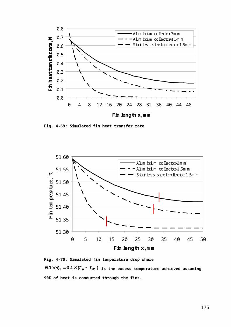
coils both working as heat-echangers, one heated by the SWH, the other heated by a

boiler. Outputs of the back-up (boiler) and the SWH systems are both into one water

tank. This type of installation is another frequently adopted alternative in the UK.

Fig. 6-105: Combined solar dwelling hot water tank.

Another method would be to use an external heat exchanger. As previously, cold water

from mains enters the bottom of the water tank but also goes to a secondary pre-heated

circuit. The secondary circuit goes into an external heat-exchanger in transferring the

heat from the primary SWH to the secondary circuit going back to the water tank. The

water uses a back-up circuit to deliver the hot water supply. Each circuit requires a

pump resulting in higher final costs. A schematic of the system is shown in Figure 6-4.

185

Fig. 6-106: External heat exchanger

Another installation proposed by AES consists of a combi-boiler solar compatible

installation shown in Figure 6-5. Cold water from the mains enters the bottom of the

water tank to be pre-heated by the SWH primary circuit used as a heat-exchanger. Each

time hot water is drawn from the household the pre-heated water goes to an

instantaneous heating appliance such as a combi-boiler which uses a thermostatic

blending valve to protect the cold supply of the combi-boiler.

186

Fig. 6-107: Combi-boiler solar compatible installation

6.2.1.3 Solartwin systems

The Solartwin system is a more recently adopted alternative using a direct solar system

installation. The SWH system shares the same open-vented safety system and cold

water reservoir with the water tank.

The SWH system employs a flexible pipe in the absorber plate resisting the volumetric

expansion due to freezing. The SWH system is therefore freeze-tolerant and can use

mains water as a heat transfer fluid. The collector and circulation system can therefore

be plumbed directly into the existing hot water system. The use of a small pump

powered by a photovoltaic module provides a low and variable flow enhancing storage

tank stratification as stated by Grassie et al (2001) and results in a net zero carbon

system. A schematic of the system is provided in Figure 6-6.

187

Fig. 6-108: Solartwin system

This system reduces costs as it requires minimal plumbing and additional components

required to prevent frost damage in the above systems are no longer necessary. It is also

easier and quicker to install and has an additional thermal benefit through heating the

domestic hot water directly.

6.2.2 Suggested installation for the ICS-SWH

Based on the typical commercial SWH installation detailed above, constraints for the

installation of the ICS-SWH under study were considerated and an optimised

installation proposed.

6.2.2.1 Installation considerations

The solar water heater under study stores the solar heat directly in its integrated tank

allowing the heat to build-up slowly during the day. Using the ICS-SWH as both the

collector and storage tank significantly reduces the space requirements and costs

associated with typical SWH installation as it would use main water. 188

The primary issues concerning the ICS-SWH installation would be the potential

freezing problems and pressurisation of the system. The system uses mains water as the

heat transfer fluid and could potentially freeze during winter months. Using a sealed

system would result in a significant increase static pressure between 1 - 3 Bar over

atmospheric pressure.

In extreme weather conditions, freezing could damage the ICS-SWH. Grassie (2001)

suggested the use of flexible ethylene propylene diene M-class rubber or EPDM rubber

instead of the more commonly used copper pipes. Using this material allows pipes to

expand during freezing periods therefore reducing potential damage. The ICS-SWH

could be designed to use EPDM rubber inlet and outlet pipes where the greatest

potential for freezing occurs. An additional benefit in using EPDM rubber inlet and

outlet pipes would be the avoidance of galvanic corrosion occurring between aluminium

and commonly used materials for water heating pipes such as copper, brass and

stainless-steel.

Using a sealed direct system would result in pressures of up to 3 Bar that the ICS-SWH

may not withstand. A pressure regulation valve and a pressure relief valve could then be

integrated in the installation to regulate the water pressure on entry to the ICS-SWH and

relieve excess pressure due to expansion.

6.2.2.2 Proposed ICS-SWH installation

The system would consist of a direct sealed installation using mains water as a heat

transfer fluid that passes through the SWH incorporating a back-up heat source to

provide required domestic hot water final delivery temperatures. A combi-boiler solar

compatible installation or direct electric heater, such as Titan 66 tankless hot water

heater, would be then integrated into the system as a back-up heat source. Smyth et al.

(2001) suggested that most ICS-SWHs have large thermal masses and simple compact

structures which give good general resistance to freezing climates. Further studies in

order to integrate tolerance to freezing are required for this system. Initial discussion

suggest a flow regime induced within the ICS-SWH and the use of flexible inlet and

outlet pipes capable of resisting the volumetric expansion due to freezing and reducing

the risk of galvanic corrosion.

189

Water quality is of primary importance if the water is being used directly from the ICS-

SWH. Limescale is a common phenomenon occurring in hot water storage systems

indirectly or directly connected to the solar water heater. The main component of

limescale deposited in water heaters consists of calcium carbonate which is soluble in

water. However, at temperatures above 70C the soluble bicarbonate is converted to

poorly soluble carbonate leading to deposits in the water heater usually resulting in a

life and performance reduction of the system. There are many ways to prevent

limescale. Products such as “Ecoflow” are reported to prevent limescale at the source. It

consists of a magnetic water conditioner fitted on the rising main where water comes

into the home providing a constant supply of magnetically treated water. The

sterilisation of bacteria such as the legionella bacteria in hot water systems is also of

primary importance for Health and Safety approval of the ICS-SWH. Temperatures of

consumable water are generally between 20C and 46C according to CIBSE (2002)

when storing heat, thus providing adequate conditions for the multiplication of bacteria.

The treatment of the pre-heated water from the ICS-SWH therefore cannot be

considered suitable for distribution as domestic hot water until fully treated. At 60C,

bacteria can survive for only minutes whereas at 70C the bacteria in the water are killed

instantaneously. A flow limiter would be required in the case of an instantaneous

heating appliance such as the ICS-SWH in order to maintain the target treating

temperature. A thermostat interlocked to the instantaneous heating appliance will also

ensure that all water draw-off reached the target temperature. A schematic of the system

is shown in Figure 6-7 including the components below:

1. Pressure regulator valve

2. ICS-SWH

3. Pressure relief valve / Air vent

4. Thermostatic mixing valve

5. Instantaneous heating appliance

6. Thermocouple

190

Fig. 6-109: ICS-SWH installation

When hot water is drawn off from the ICS-SWH, mains cold water controlled by a

pressure regulated valve is fed to the bottom of the ICS-SWH flushing out the hot water

from the top of the collector passing through a pressure relief valve. The hot water then

goes to an instantaneous heating appliance such as a combi-boiler or electric heater to

deliver the desired temperature of hot water supply.

This system would reduce costs as it requires minimal plumbing; it is of simple

construction and heats the domestic hot water directly using no separate water tank.

Supposing that the ICS-SWH was integrated in a zero-carbon house, the electric

instantaneous heating device could be powered by micro-renewable technologies;

therefore resulting in a zero-carbon system.

6.3 Integration of the ICS-SWH into roof structure

Integrating solar water heaters into roofs depends considerably on the roof type and the

design of the solar water heater installed. Most solar water heaters in UK are mounted

above the roof covering using brackets to hold the collector to the roof structure. The

roof is therefore altered from its original design loading which might cause structural

and durability issues. Solar water heaters can also be vertically mounted or integrated

directly into the roof covering but this would require specialist structural advice.

Penetrations for bracketry and water connection also compromise the roof integrity.

1

2

3

4

5

6

191

Current estimates from the Parliamentary Office of Science and Technology – POST

(2003) assert that there will be three million new UK households by 2016. The UK

government is encouraging a modern modular method of construction (MMC), which it

says can achieve “a step change in the construction industry to produce the quantity and

quality of housing we need” as stated by POST (2003).

In order to provide the best practice to integrate the ICS-SWH in future households, an

overall insight of MMC and more specificallyan example of this, the structural

insulated roofing system (SIRS) developed by a Scottish based company Donaldson

Timber Engineering (2007) is presented to demonstrate its integration.

6.3.1 Modern Method of Construction (MMC)

The recent interest in MMC for housing construction is driven by a growth in the

number of households in the UK. MMC, also known as prefabrication, consists of the

manufacturing of house parts off-site in factories. While issues have arisen regarding

the quality of houses, recent technical improvements in prefabrication including

innovative site-based methods and the wide range of material used, suggests that MMC

has many advantages with potential benefits described by POST (2003) such as:

- faster construction

- fewer housing defects

- energy efficient houses

- reductions in energy use (less transport)

- less waste production

- safer working conditions

- lower impact on local residents during construction

The two main products of MMC consist of modules and panels. Modules, also known

as pods, consists of ready-made rooms, usually bathrooms or kitchens where all the

fittings and services are added in the factory. Ready-made rooms are then assembled

together to produce a whole dwelling. Panels consist of ready made walls, floors or

roofs. These are transported to the site and can often be assembled within a day as

stated by English Partnership (2007).

192

6.3.2 SIRS Roofs

The SIRS roof (Structural Insulated Roof System), manufactured by Donaldson Timber

Engineering (DTE) is an example of modular offsite roof design, employing modern

methods of construction MMC. The SIRS roof is a roofing system that has been

developed to provide a safe and cost effective solution in delivering additional space

such as room in the roof in a domestic dwelling.

The SIRS roof design parameters exceed current building regulations in terms of

insulation, and comply with government directives on modern methods of construction.

The SIRS system suits a variety of roof shapes and is manufactured using timber from sustainable sources. It also contributes to Low Carbon Build and has been approved by the NHBC (National House-Building Council) last July 2007. The SIRS roof assembly is shown in Figures 6-

8 and 6-9.

Fig. 6-110: Structural Insulated Roof System - SIRS, Wood (2006)

193

Fig. 6-111: Structural Insulated Roof System, James Johns roof trial.

The design flexibility of the SIRS roof would allow the direct integration of the ICS-

SWH on the roof panel. This would result in a faster and safer integration of renewable

technology through off-site construction and high insulation of the ICS-SWH due to the

excellent insulation performance of SIRS.

6.3.3 Structural issues

There are many structural issues when considering the installation of a SWH system.

The additional load of the mounted ICS-SWH requires specialist structural advice.

However, directly integrating the ICS-SWH into the roof covering replaces tiles thereby

reducing weight issues. For instance, the Sandtoft company (2008) provides a range of

clay tiles weighing between 34-72kg for a 1m2 area resulting in an average weight of

53kg/m2. When integrated into the roof covering the filled 1m2 AL-1.5 ICS-SWHs

weighs 41.3kg which would result in a 22.1% weight reduction over clay tiles.

A structural engineer would normally be responsible for calculating such loads. As a

result of high wind speed, steeper pitched roofs are generally installed in Scotland to

diminish the potential for tiles lifting.

194

Whether the installation is mounted above the roof or directly integrated into the roof

covering, a flashing system would be required to make the installation weatherproof. An

overview of VELUX (2005) flashing systems is given as suitable method for the ICS-

SWH integration in roofs. VELUX flashings ensure weathertight installation of all

VELUX roof windows by ensuring safe water drainage from the roof above the

window. VELUX (2005) uses prefabricated flashing systems which overlap with the

roof covering to provide a weathertight finish around roof windows. VELUX flashing

systems are compatible with most types of roofing material and allow a discrete

installation as the roofing material covers the top and side flashing components.

Flashing materials are weather-resistant. A collar ensures a tight connection between the

roof window and the membrane and weather tight joints are created by overlapping the

flashing components whilst the foam gasket creates a seal between the flashing and the

roofing materials. Another feature of VELUX flashings is the incorporation of tile

support ensuring that the roofing material remains in the right inclination above the roof

window. A pleated apron is then dressed to form a tight seal underneath the window in a

profiled roof. Figure 6-10 shows a VELUX installation.

Fig. 6-112: Installation schematic and final installation of VELUX windows, VELUX (2005)

The general good practice introduced by CIBSE (2007) in respects of pitched roof guidance is:

- To maintain access to the roof covering below the solar water heater

- To report loads onto the roof covering195

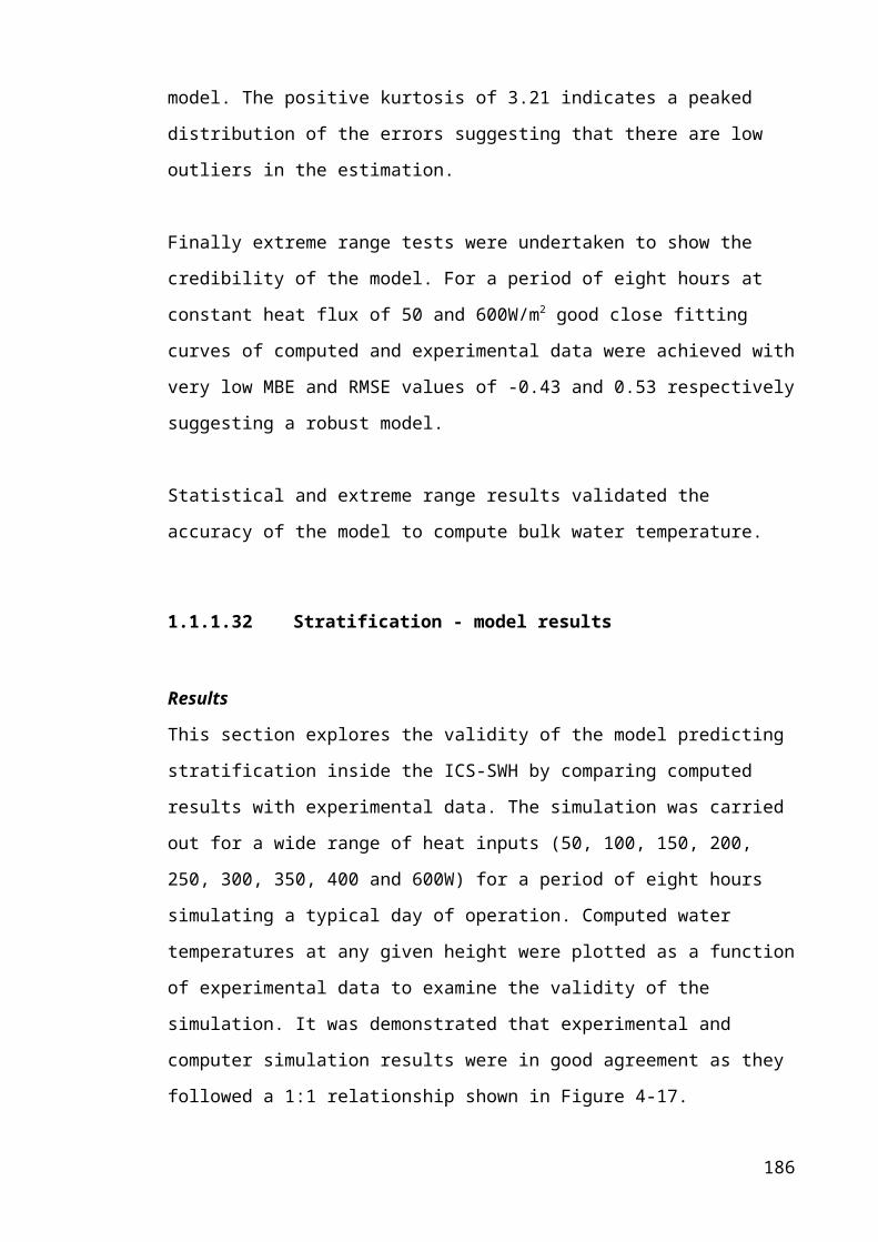
- To design the loads onto substantial roof structures such as trusses

- To provide sufficient lap of flashing where tiles are cut or raised- To consider negative pressure lifting adjacent components such

as tiles Based on these parameters, the integration of the ICS-SWH was considered and simulated.

6.3.4 Integration of the ICS-SWH

The integration of any SWH has a direct impact on a building including its performance

and aesthetics. Integrating an ICS-SWH should not devalue the property and should

comply with building regulations and planning.

Using VELUX methods for weatherproofing the ICS-SWH in a SIRS roof structure

could ensure a good integration of the ICS-SWH in a roof covering. However there are

issues concerning the direct integration of the ICS-SWH into the roof covering. The

viability of such integration should be studied further in order to ensure its feasibility.

6.4 Concluding remarks

This chapter explored the potential installation and integration of the ICS-SWH under

study into recent advances in constructions practice. Recent governmental initiatives

towards the expansion of zero-carbon development enhanced the integration of micro-

generation technologies into buildings. The best practice examples of low and zero-

carbon developments such as the Kingspan Lighthouse or RuralZED identified the

potential for roof mounted SWHs to generate a dwellings water heating with a heating

back up and their contribution towards such zero-carbon developments. Best SWH

installation practices of three Scottish companies were studied in order to provide an

optimum practice for the ICS-SWH installation. The suggested installation consisted of

a direct sealed system using mains water as a heat transfer fluid and an instantaneous

heating back-up source such as a Titan 66 tankless hot water heater.

The integration of the ICS-SWH in future potential Scottish household is a final

milestone of the research project. Integrating an ICS-SWH should not devalue the

property and should contribute to complying with housing codes and legislations.

196

Modern methods of construction and more precisely of structural insulated roofing

system (SIRS) were recently introduced as contributing to Low Carbon Build. The design flexibility of the SIRS roof could allow the simulated direct integration of the ICS-SWH inside the roof panel. Such installation results not only in faster and safer integration through off-site construction, but also in higher performance of the ICS-SWH due to the high insulation performance of SIRS. Such installation would also provide a

substantial value to developers proposing such pre-integrated micro-renewable systems

to customers resulting in achieving higher levels of the Code for Sustainable Homes.

In conclusion, this section of the thesis opens an avenue for future work on ICS-SWH

integration but also shows the potential of ICS-SWH in the solar water heating and

zero-carbon home markets.

197

CHAPTER 7 CONCLUSIONS

Energy plays an essential role in society and human life, driving economic development

and the wellbeing of society. Modern societies use more energy every year for industry,

services, homes and transport resulting in increased environmental concerns associated

with fossil fuel consumption and production. Ensuring a secure, clean and affordable

supply of energy is essential towards the sustainable development of a modern society.

The domestic sector is the largest consumer of energy in the UK with 80% accounting

for space and water heating. Hence, there is good potential scope for addressing

domestic energy requirements, particularly for hot water, from renewable sources. Solar

water heating systems have real potential in Scotland due to the higher annual heating

loads allowing longer and greater savings using solar thermal energy. A review of many

years of research on solar water heating systems has outlined the promising approach of

integrated collector storage solar water heaters (ICS-SWH) in northern hemisphere

applications due to their good overall performance in overcast sky conditions. ICS-

SWHs are one of the simplest types of SWH on the market incorporating the solar

collector and thermal storage tank in a single unit making them relatively affordable

with low costs. There was therefore a need to estimate the potential of ICS-SWH for the

northern climates.

This research was conducted with the primary goals of developing an affordable,

optimised and feasible ICS-SWH prototype for Scottish weather conditions and to

develop a new tool to model ICS-SWH performance. The approach involved laboratory

and field tests of the ICS-SWH, performance modelling for laboratory and field

conditions, performance optimisation through CFD modelling, life cycle assessment and

monetary analysis of the ICS-SWH and finally the analysis of potential benefits and

integration into buildings of this ICS-SWH prototype.

7.1 Summary of conclusions

Significant points that can be drawn from the research analyses are as follows:

Laboratory and field experiments

- The methodology adopted in this study was generally more accurate and rigorous than

previous studies.198

- The incorporation of extended surfaces in the ICS-SWH was analysed and suggested

an increase in heat transfer and water stratification in the ICS-SWH as well as providing

structural strength to the collector. Incorporating fins in the collector resulted in an

increase in heat transfer of 18% in the stainless-steel ICW-SWH. Using a more

conductive material, such as aluminium, resulted in a 13% increase in water

temperature.

- Analysis suggested that the temperature stratification profile results in differential

buoyancy forces in the fluid causing convection by gravity. It also indicated that this

depends upon the incident solar radiation, the exposure time and collector material,

given a constant angle of inclination of the ICS-SWH. A polynomial function for the

stratification profile for each hour could then be developed taking heat flux and

longitudinal location in the collector as the main parameters.

- The benefit of selecting aluminium for the ICS-SWH was clearly supported by the

current laboratory findings; showing it out-performing the stainless-steel ICS-SWH

with an overall increase in the aluminium ICS-SWH efficiency of 6% over an eight

hour time period.

Although the collector was tested in a laboratory with calibrated instruments, the actual

performance of the ICS-SWH under real weather conditions yielded important results

on assessing the viability of the aluminium ICS-SWH and are summarised below.

- Parameters such as thermal mass of the system, orientation, cloud cover and sky

temperature were found to significantly influence the ICS-SWH performance in field

weather conditions, and should not be neglected.

The thermal mass was found to play an important role in the effectiveness of the system

as it affected the heating charge and cooling discharge operations of the collector and

the amount of stored thermal energy. The water stored in the collector chiefly

contributed towards the thermal mass of the system with a value of 208.3kJ/K compared

with the aluminium and stainless-steel material of heat capacities of 17.2 kJ/K and

13.3kJ/K respectively. This shows the ability of a given water volume to store internal

energy while undergoing a given temperature change.

199

It was also observed that a decrease in incident solar radiation for a relatively long

period of time can lead to significant losses and decrease in stratification rate, therefore

positioning of the ICS-SWH is of primary importance to achieving good performances.

The effective sky temperature can be about 10-20 degrees Celsius below ambient

temperature at ground level with clear sky conditions and close to, or just below, the

ambient temperature during cloudy conditions. It was therefore concluded that cloud

cover should not be neglected as it affects the cover temperature through radiation

losses and therefore the final water temperature output of the ICS-SWH.

- The draw-off study showed that the ICS-SWH was able to maintain temperature

stratification when draw-off occurs, a crucial factor in maintaining good performance of

the ICS-SWH. It was also observed that draw-off actually increased the overall thermal

longitudinal stratification, thus improving the overall performance of the ICS-SWH.

Average draw-off temperatures recorded at peak demand hours suggest that the ICS-

SWH could cover 55%, 66%, 83% 72% of the hot water demand at 8:00, 9:00, 19:00

and 20:00 respectively based on a delivery temperature of 55°C. A strong relationship

between water drawn-off, water temperature stratification, solar radiation and outlet

water temperature achieved in the collector was reported.

- In addition to the relative importance of different parameters influencing the ICS-

SWH performance developed in this study, the current conventional standard procedure

used by the ESCSTG (1989) for predicting the effectiveness of ICS-SWH was found

not to be representative of the actual system performance as thse assume steady state

conditions. This emphasised a need for new methods to predict water temperatures and

performance of ICS-SWH.

Modelling ICS-SWH performances

- Two macro models - laboratory and field - were developed in this study to predict the

performance of ICS-SWHs at any location and with different installation configurations.

Each macro model resulted in a thermal energy simulation model which analysed

combined heat flux environmental networks within the ICS-SWH.

- The laboratory macro-model was able to predict the bulk water temperature in

different ICS-SWH configurations using different construction materials for a given

200

heat flux, ambient temperature, inlet water temperature and resultant stratification

profile over time.

The role of extended heat transfer surfaces (fins) were modelled and showed good

improvement by achieving higher bulk water temperatures. Effective fin heat transfer

rates were enhanced by the choice of a material e.g. aluminium over stainless steel. The

improvement was found to be 67.3% and 63% for aluminium fins of 3mm and 1.5mm

thickness and 25.3% for 1.5mm thick stainless-steel.

An improvement factor (IF) measuring the improvement achieved by using fins in the

ICS-SWH was developed. By increasing the thickness of the fins the overall IF

improved by 3.5%, while changing to a more conductive material the IF improved by

5.5%. The greatest improvement factor was achieved for the aluminium ICS-SWH with

a 3mm fin thickness.

The computational results from the model were found to be in close agreement with the

experimental data. Satisfactory curve fits were obtained for the water temperatures,

achieved experimentally and numerically for all the ICS-SWH types. Testing the results

using statistical methods resulted in very low MBE and RMSE values; validating the

ability of the model to predict the water bulk temperature in the ICS-SWH.

Longitudinal stratification of temperature within the solar collector was modelled using

the mean bulk water temperature computed by the macro model, the given heat flux and

the total time of exposure. The stratification model was developed using polynomial

functions previously developed via experimental data for 100, 200 and 400W/m2.

Different heat inputs outside the normal experimental range were then simulated in

order to validate the model. Results for 50, 150, 250, 350 and 600W/m2 over a period of

eight hours (simulating a typical day of operation) demonstrated that experimental and

computer simulation results were in good agreement. The MBE value of 1 Celsius

showed that the model had a tendency to slightly under predict its computed value.

Statistical results validated the accuracy of the model to compute bulk water

temperature.

- The field macro thermal model developed was found to be suitable for predicting bulk

water temperatures under real weather conditions and therefore more predictable ICS-

SWH performance.

Analysis carried out using data for five and fifty day testing periods between the month

of June and July validated the model to predict bulk water temperature inside the ICS-

SWH by comparing computed results with experimental data.

201

It was observed that gradual heating and cooling profiles due to the thermal mass of the

system were experienced in the macro model. However, a lower cooling rate of the

modelled values was observed for each day. This could be explained by the propagation

of errors and uncertainty by the use of regression analysis and assumed weather data;

resulting in a decrease in the accuracy of the model.

Experimental water temperature was followed very closely by predicted water

temperature although it showed a slight over-estimation of 1.3 and 1.5 Celsius of its

computed values by the proposed model for five and fifty day periods respectively. The

study also demonstrated the effect of wind velocity on the bulk water temperature and

the importance of having accurate wind speeds. Increasing the velocity from 0m/s to

6m/s resulted in an average decrease of 5% of the bulk water temperature.

Although this model only gives mean values of water temperature which, in reality,

varies along the longitudinal height of the collector, it gave a good estimation of the

ICS-SWH performance. The simulation could be extended resulting in a useful tool to

estimate the yearly performance of the ICS-SWH.

- Both simulation models showed that computational results were found to be in close

agreement with the experimental field measurements. Statistical methods suggested that

both models were robust and could compute bulk water temperature in the ICS-SWH

and predict the performance of an ICS-SWH at any location and with different

installation configurations.

Optimisation through CFD modelling

- A Computational Fluid Dynamic (CFD) study was undertaken to model flow and heat

transfer in the three-dimensional (3D) SWH geometry to provide information about

performance of the collector and evaluate design improvements. It was found that 2D

analysis was insufficient for any angle of inclination of the ICS-SWH above horizontal

as a gradient exists in the longitudinal direction. Hence, based on a 45° inclination of

the collector, a 3D analysis was undertaken to estimate an optimum fin spacing to make

further improvements on the original four-fin ICS-SWH.

- It was found that one further fin added to the original four-fin ICS-SWH design would

improve the heat transfer by 2.3%. It was observed that the five fins supplied more

energy to the collector than four at the beginning of the charging process. The

202

intermittent availability of incident solar radiation in Scotland shows high potential for

this type of improvement as it is advantageous to have a rapid heating process.

- It was also observed that while the five fins supplied more energy to the collector than

four at the beginning of the charging process, additional fins seriously impeded the

water flow with a decrease of the velocity in the SWH. This decrease in velocity has a

corresponding reduction on the Nusselt number with a consequence that the heat

transfer coefficient falls in a predictable manner as outlined by Churchill (1974).

Life cycle assessment and monetary payback

- A LCA and monetary analysis of two aluminium ICS-SWHs of 1.5 and 3mm

thickness (AL-1.5 and AL-3) and one stainless-steel ICS-SWH of 1.5mm (ST-1.5)

incorporating extended heat transfer surfaces were carried out in order to establish the

most commercially viable ICS-SWH with the smallest environmental footprint.

- It was found that despite the high amount of energy to produce aluminium, the “light”

and recyclable properties of the material resulted in similar embodied energy when

compared with stainless-steel. This resulted in a smaller environmental impact due to

lower carbon emissions released to the atmosphere during the production process.

Energy and carbon dioxide savings associated by using those ICS-SWHs were modelled

and showed that although the AL-1.5 ICS-SWH was marginally out-performed (0.1%)

by the AL-3 ICS-SWH, the fact that it only uses half the volume of material in

producion makes it more viable. The carbon dioxide savings showed that, depending on

the ICS-SWH installed, there is a potential for saving 6% more kgCO2 per year by using

an Al-1.5 compared with a ST-1.5, and only 0.5% by increasing the thickness of a

similar ICS-SWH material.

The energy payback times (EPBT) of the ICS-SWHs were found to be consistently

lower than three years for all ICS-SWHs with the lowest EPBT value of 1 year 7

months achieved by the AL-1.5 ICS-SWH. This value shows the great energy potential

of such an ICS-SWH design. A calculation of the carbon dioxide emission payback

times confirms the higher potential of using an AL-1.5 ICS-SWH by decreasing the

ECPBT by 42% and 48% when compared with AL-3 and ST-1.5 ICS-SWHs

respectively.

203

The potential annual monetary savings of a 3m2 ICS-SWHs installation vary

considerably between homes using fossil fuelled or electric heating systems.

Partially replacing a gas heating system with an ICS-SWH would result in a maximum

monetary payback period (MPBP) of 28.4, 12.2 and 6.1 years for the ST-1.5, AL-3 and

AL-1.5 respectively considering the collectors’ capital cost only. Assuming ICS-SWH

capital costs including all the components for installation resulted in increasing MPBT

of 23, 39 and 57% for the ST-1.5, AL-3 and AL-1.5 respectively. In both MPBT studies

the AL-1.5 ICS-SWH was found as the most viable solution. The ST-1.5 ICS-SWH was

a less attractive or viable alternative when installed in conjunction with a gas central

heating system as the customer would not realise any significant economic benefit over

its estimated life time of 20 years.

- All results point to the AL-1.5 ICS-SWH as the most viable alternative to operate in

Scottish weather conditions. It would therefore be recommended to use an AL-1.5 ICS-

SWH for further investigations due to its energy and environmental benefits.

Integration and potential benefits

This section explored the potential installation and integration of the ICS-SWH under

study into recent advances in constructions practice and its potential benefits for

builders and households.

- It was found that recent government initiatives in the UK help support developers

towards the expansion of zero-carbon development and enhanced the integration of

micro-generation technologies into buildings. Roof mounted SWHs were found to be

installed in many best practice examples of low and zero-carbon developments such as

the Kingspan Lighthouse or RuralZED suggesting that there is a strong potential for this

type of technology to participate towards zero-carbon homes.

- Based on the predominantly installed commercial types of flat-plate collector in

Scotland, best practice for installing the ICS-SWH appeared to be a direct sealed

installation. This installation would use mains water supply as the heat transfer fluid

backed-up by an ‘instantaneous’ in-line heat source for periods of low insolation or as

top-up heating provision.

204

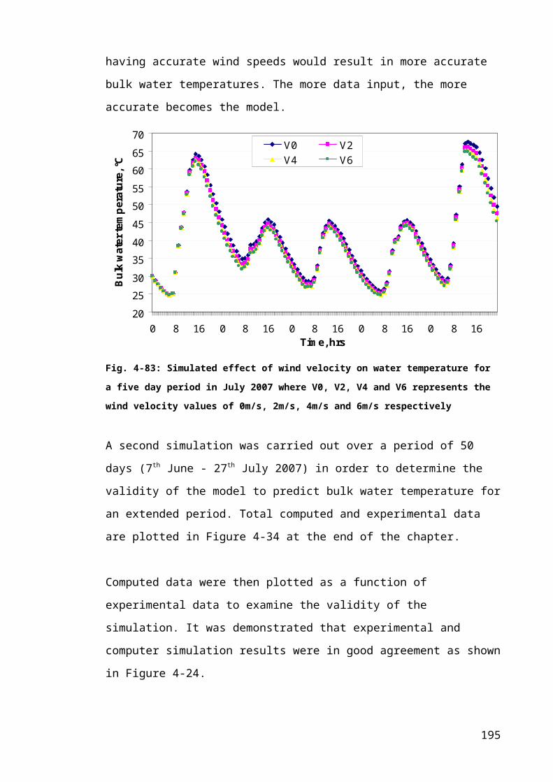
- Potential for integrating the ICS-SWH in future Scottish dwelling design was a final

milestone of this research project. It was found that modern methods of construction

and, more specifically, examples of structural insulated roofing system (SIRS) or

Structural Insulated Panels (SIPS) were recently introduced as contributing to Low Carbon Build and could allow the direct integration of the ICS-SWH inside the roof panel. Thus contributing to complyiance with planning and

building regulations. Such installation would result not only in faster and safer integration, through off-site construction, but also in higher performance of the ICS-SWH due to the high insulation performance of

such roof systems. This would also provide a substantial value to developers

proposing such pre-integrated micro-renewable systems to customers resulting in

achieving higher levels of the Code for Sustainable Homes.

7.2 Contribution to knowledge

Original contribution within the context of the presented research can be identified in

the following sub-sections:

Innovation:

The collector investigated is a new prototype enhancing the thermal efficiency of the

ICS-SWH through the use of more efficient materials while lowering the capital costs

down to the order of £300 compared to commercially available collectors priced at over

£2500.

Methodology and feasibility:

Laboratory and field experiments provided detailed information of the ICS-SWH

behaviour in different situations. The field experiments showed the feasibility of such

heaters in Scottish weather conditions. Typical annual savings of 1106 kWh can be

achieved for a 3m2 domestic system corresponding to a maximum annual saving of £40

while partially replacing a gas heating system with an ICS-SWH, and up to £134 while

replacing an electric heating system.

New predicting tool:

The innovative modelling tool developed can predict the bulk water temperature of the

ICS-SWH for any location in the world and therefore predict the ICS-SWH

205

performance. ICS-SWH design parameters can be changed by the user for their own

research resulting in an evolving programme.

Design improvement & Costs:

Improvements of the ICS-SWH design were suggested through the CFD analysis while

keeping the costs to a minimum.

Viable prototype:

The ICS-SWH prototype showed a high commercial potential due to its environmental

and monetary benefits resulting in a viable commercialisation of the prototype.

Improvements to the ICS-SWH design were also suggested through the LCA while

lowering the capital cost of the final unit.

Viable installation:

The ICS-SWH prototype showed potential for integration into commonly used solar

water heating installations which could result in a viable installation. This type of

installation could use an electric instantaneous hot water heater as an instantaneous

back-up heater.

Market value:

The ICS-SWH was shown to have a real market value. To date, there is no commercial

ICS-SWH on the solar thermal market resulting in a niche product. The confidence in

the design resulted in patenting the ICS-SWH. The ICS-SWH could also have a high

market value when integrated into modern methods of construction such as roof panels.

7.3 Potential future work: Looking back, looking ahead

The avenues for possible future research can be classified as follows:

Thermal macro model potential improvements

The thermal macro model developed could be implemented in the Visual Basic program

and could provide a better user interface. Further improvements of the thermal model

could be incorporated. The thermal stratification model could be developed for real

weather conditions. Other improvements such as the modelling of water draw-off could

be integrated.

206

Further CFD modelling

In light of the CFD modelling results presented, the five-fin collector performed

generally better than the original four-fin collector. Therefore, this design could be

suggested as a new arrangement for the collector assuming that the addition of one fin

has a very low additional cost. The LCA study also recommended the use of an

aluminium ICS-SWHs of 1.5 thickness incorporating extended heat transfer surfaces for

further investigations due to its energy and environmental benefits. Future work could

then be carried out through CFD analysis for a five fin aluminium ICS-SWH of 1.5mm

thickness. Further study assessing the structural integrity of the aluminium ICS-SWHs

of 1.5 thickness should also be undertaken.

Life cycle assessment – going further

The eco-profile of an ICS-SWH would be different for any given location in the world.

Scotland being a marginal weather location, somewhere with greater solar radiation

potential would result in a better eco-profile of the ICS-SWH by achieving greater

energy savings and therefore further reducing carbon emissions. This ICS-SWH would

therefore have better applications in a sunnier climate.

The variability between LCA studies makes the comparison between studies difficult.

However, it would be interesting to aggregated indices such as Tsilingiridis et al (2004)

in future LCA research in order to compare with other studies.

Potential integration – going further

Health and safety issues should be addressed in order to show the actual potential of the

ICS-SWH integration into dwellings and the fulfilment of the health and safety

constraints towards such systems. Other issues such as planning permissions constraints

could be assessed.

The integration of any SWH has a direct impact on a building including its performance

and aesthetics. Integrating an ICS-SWH should not devalue the property and should

contribute to achieve planning and regulatory requirements. Therefore further study on

integration of such heaters in SIRS roof structure would be recommended.

The integration of the ICS-SWH into a trial house would be a good step in order to

conduct seasonal performance with draw-off. Such a study of the ICS-SWH could be

conducted in Scotland to assess the actual potential of the collector throughout the year.

207

REFERENCES

APPENDICES

208

APPENDIX A: GLOSSARY OF TERMS

APPENDIX B: LIST OF PUBLICATIONS

APPENDIX C: THERMAL MODELS

209

APPENDIX A

GLOSSARY OF TERMS

Energy mix: The combination of sources used to provide energy at any given time and

place.

Traditional biomass: It represents unprocessed biomass including forest product waste,

collected fuel wood, agricultural waste and animal dung that are burned in stoves or

furnaces to provide heat energy for cooking, heating and agricultural and industrial

processing, typically in rural areas.

Degree-days: The rate of heat loss from a building, (related to the building fabric) and

the temperature difference between the inside and outside of a building - the greater the

temperature difference the more heat will be lost.

Atmospheric transparency window: The atmosphere behaves like a black body

throughout the infrared spectrum with the exception of the wavelength interval between

8 -14m. The so-called Atmospheric Transparency Window is located between these

two extremes and is characterised by a high transparency to infrared thermal radiation

and therefore by low energy emission.

Environment: The term environment represents the external conditions including

temperature, wind speed, irradiation, cloud cover etc with which the SWH interacts.

Clear sky index: Corresponding to the ratio of the global horizontal irradiance to the

global horizontal irradiance under clear sky conditions.

Solar fraction: The solar fraction is the amount of energy provided by the solar

technology divided by the total energy required.

210

APPENDIX B

LIST OF PUBLICATIONS

Currie, J.I., Garnier, C., Muneer, T., Henderson, D., Grassie, T. (2007) Comparison of

Finned Aluminium and Steel Integrated Collector Storage Solar Water Heater,

SOLARIS 2007, 3rd International Conference on Solar Radiation and Day Lighting,

New Delhi.

Currie, J.I., Garnier, C., Muneer, T., Grassie, T., Henderson, D. (2008) Modelling bulk

water temperature in integrated collector storage systems. Building Services

Engineering Research and Technology (Published)

Garnier, C., Currie, J.I., Muneer, T. and Girard, A. (2008) Computational study of an

integrated collector storage solar water heater, EUROSUN 2008, International

Conference on Solar Heating, Cooling and Buildings, Lisbon.

Garnier, C., Currie, J.I. and Muneer, T. (2008) Integrated collector storage solar water

heater: Temperature stratification. Applied Energy (Accepted for publication)

Garnier, C., Currie, J.I. and Muneer, T. (2008) Integrated collector storage solar water

heater: Life Cycle Assessment. Journal of Cleaner Production (Communicated for

publication)

Garnier, C., Muneer, T. and Currie, J.I. (2008) Mathematical modelling of integrated

collector storage systems under real weather conditions. American Society of

Mechanical Engineers (Communicated for publication)

211

APPENDIX C

SOLAR THERMAL ENERGY SYSTEM FOR HOUSING (STESH)

FIELD THERMAL MODELS

STESH – Field model program

Fig. C1: Caption of STESH programme welcome page

Sub compute01()

Collsize = Sheets("Site-System Input").Range("G22").Value

Depth = Sheets("Site-System Input").Range("G23").Value

Thickness = Sheets("Site-System Input").Range("G24").Value

Longueur = Sheets("Site-System Input").Range("G25").Value

Volume = Collsize * Depth

Ac = Longueur * Thickness

Peri = 2 * (Thickness + Longueur)

finarea = 0

' Depends on choice

If Sheets("Site-System Input").Range("G27").Value = "No" Then finarea = 0

212

If Sheets("Site-System Input").Range("G27").Value = "Yes" Then finarea = 4 * 0.002 *

Longueur

InTw = Sheets("Site-System Input").Cells(19, 7).Value + 273.15

Sheets("Site-System Input").Cells(20, 7).Value = InTw

Tw = Sheets("Meteorological Input").Cells(8, 21).Value 'Site-System Input water temp.

For x = 8 To 127

Tam = Sheets("Meteorological Input").Cells(x, 6).Value

Vel = Sheets("Meteorological Input").Cells(x, 7).Value

CloudCover = Sheets("Meteorological Input").Cells(x, 8).Value

RefMidnight = Sheets("Meteorological Input").Cells(x, 3).Value

Ep = 0.95

Aw = 1 'm2

Angle = Sheets("Site-System Input").Range("H14").Value

Gin = 0.8 * Sheets("Meteorological Input").Cells(x, 20).Value

mcp = Sheets("Site-System Input").Cells(29, 7).Value

kmaterial = Sheets("Site-System Input").Cells(30, 7).Value

mcwater = 208.323 'kJ/K

mcinsul = 2.897 'kJ/K

mcwood = 37.32 'kJ/K

mcglazing = 10.56 'kJ/K

mcin = 3.37637 'kJ/K

Ta = Tam + 273.15

'Tsky = Ta

hwind = 8.55 + 2.56 * Vel

Eg = 0.88

' Initialisation of Tp & Tc

Tp = Tw + 0.5

Tc = Tp - ((Tp - Ta) / 3)

deltime = 360

For iminute = 1 To 10

'Start iterative loop

For i = 1 To 10

213

Tdpclear = (0.7105 * (Ta - 273.15) - 0.7864)

Tdpovercast = (0.8231 * (Ta - 273.15) - 0.8119)

If 0 <= CloudCover < 3 Then

Tdp = Tdpclear

EmisS = 0.747 + 0.594 * (Tdp / 100) - 0.551 * ((Tdp / 100) ^ 2)

If 3 <= CloudCover <= 5 Then

Tdp = (Tdpclear + Tdpovercast) / 2

EmisS = (0.747 + 0.594 * (Tdp / 100) - 0.551 * ((Tdp / 100) ^ 2)) * (1 + 0.0224 * 0.5

- 0.0035 * (0.5 ^ 2) + 0.00028 * (0.5 ^ 3))

If 5 < CloudCover Then

Tdp = Tdpovercast

EmisS = (0.747 + 0.594 * (Tdp / 100) - 0.551 * ((Tdp / 100) ^ 2)) * (1 + 0.0224 -

0.0035 + 0.00028)

End If

End If

End If

Esky = 1 + ((107952 * (1 - EmisS)) / ((Ta ^ 2) - 680.8 * Ta + 73594.9)

Fsky = 1 / ((1 / Eg) + (1 / Esky) - 1)

CoordoA = 15 * RefMidnight

CoordoB = 0.711 + 0.0056 * Tdp + 0.000073 * Tdp ^ 2

CoordoC = Cos((CoordoA) ^ (1 / 4))

Tsky = Ta * (CoordoB + 0.013 * CoordoC)

Ucar = (Fsky * 0.0000000567 * (Tc ^ 4 - Tsky ^ 4)) / (Tc - Tsky)

Ucac = hwind

Uca = Ucac + Ucar

BEmm = (1 / Eg) + (1 / Ep) - 1

Upcr = (0.0000000567 * (Tp + Tc) * (Tp ^ 2 + Tc ^ 2)) / BEmm

'Calculation of Rayliegh number for air cavity

Tfag = (Tp + Tc) / 2

214

Sheets("AirProp").Range("J13").Value = Tfag

visair = Sheets("AirProp").Range("Q18").Value

kfag = Sheets("AirProp").Range("R18").Value

visair = visair * 0.000001

Raag = (9.81 * (1 / Tfag) * (Tp - Tc) * 1 ^ 3) / (visair)

'Calculation of Nu for air cavity by Holland Regression

term1 = 1.44 * (1 - (1708 / Raag * Cos(Angle)))

term2 = 1 - ((1708 * Sin(1.8 * Angle) ^ 1.6) / (Raag * Cos(Angle)))

term3 = ((Raag * Cos(Angle) / 5830) ^ (1 / 3)) - 1

term4 = Application.Max(term1, 0)

term5 = Application.Max(0, term3)

Nuag = 1 + term2 * term4 + term5

'calculation of total conductance form plate to glass cover

Upcc = Nuag * kfag * 0.001 / (0.025)

Upc = Upcc + Upcr

'Calculation of Rayleigh Number for Water

Sheets("WaterProp").Range("Q24").Value = 0.5 * (Tw + Tp)

Speheatw = Sheets("WaterProp").Range("AA29").Value

Betaw = Sheets("WaterProp").Range("AJ29").Value

Prw = Sheets("WaterProp").Range("AK29").Value

Visw = 0.000001 * Sheets("WaterProp").Range("AC29").Value

denw = Sheets("WaterProp").Range("W29").Value

kw = 0.001 * Sheets("WaterProp").Range("AE29").Value

Raw = Prw * 9.81 * Betaw * 0.000001 * (1 ^ 3) * (Tp - Tw) / ((Visw / denw) ^ 2)

If (Raw <= 0) Then Raw = Sqr((Raw) ^ 2)

'Calcuating water conductance

Nuw = 0.56 * ((Raw * Cos(Angle)) ^ 0.25) * ((1 / 0.05) ^ (1 / 6))

hw = Nuw * kw / 1

Uw = hw

'Back losses

UAbloss = 0.35

215

' Iterations for Tp & Tc

Tp = (Gin + Upc * Tc + Uw * Tw) / (Upc + Uw)

Tc = (Upc * Tp + Ucac * Ta + Ucar * Tsky) / (Upc + Ucac + Ucar)

Next i

Qpw = Uw * (Tp - Tw)

Qpc = Upc * (Tp - Tc)

'Fin lengh calculation and improvement factor

smallm = 335 * 2 * (Longueur + Thickness) / (kmaterial * Longueur * Thickness)

smallm = Sqr(smallm)

ml = smallm * Depth

BigM = Sqr(335 * Peri * kmaterial * Ac * (Tp - Tw))

'Af = 2 * (Depth * Thickness) + 2 * (Depth * Longueur) + (Longueur * Thickness)

For j = 7 To 32

Length = Sheets("Fin Effect").Cells(j, 1).Value

tetab = Application.Cosh(ml)

teta = Application.Cosh(smallm * (Depth - (Length * 0.001)))

tetax = (teta / tetab) * Abs(Tp - Tw)

Tfin = tetax + Tw

Rafin = Prw * 9.81 * Betaw * 0.000001 * ((Depth / Cos(Angle)) ^ 3) * (Tfin - Tw) /

((Visw / denw) ^ 2)

Nufin = 0.68 + (0.67 * Rafin ^ 0.28) / (1 + (0.492 / Prw) ^ (9 / 16)) ^ (4 / 9)

hfin = Nufin * kw / (Depth / Cos(Angle))

Qxfin = hfin * (Tfin - Tw) * finarea

Sheets("Fin Effect").Cells(j, 2).Value = tetax

Sheets("Fin Effect").Cells(j, 3).Value = Tfin - 273.15

Sheets("Fin Effect").Cells(j, 4).Value = hfin

Sheets("Fin Effect").Cells(j, 5).Value = Qxfin

tetao = Sheets("Fin Effect").Cells(7, 3).Value - Sheets("Fin Effect").Cells(32, 3).Value

limittetao = 0.1 * tetao

Sheets("Fin Effect").Cells(7, 6).Value = tetao

Sheets("Fin Effect").Cells(7, 7).Value = limittetao

216

'Fin Effeciency

Lc = (Length * 0.001)

mLc = smallm * Lc

Ap = Lc * Thickness

Fineffi = Application.Tanh(mLc) / (mLc)

Sheets("Fin Effect").Cells(j, 15).Value = Fineffi

Next j

Dim D(25)

Dim E(25)

D(0) = Sheets("Fin Effect").Cells(7, 1).Value

D(1) = Sheets("Fin Effect").Cells(8, 1).Value

D(2) = Sheets("Fin Effect").Cells(9, 1).Value

D(3) = Sheets("Fin Effect").Cells(10, 1).Value

D(4) = Sheets("Fin Effect").Cells(11, 1).Value

D(5) = Sheets("Fin Effect").Cells(12, 1).Value

D(6) = Sheets("Fin Effect").Cells(13, 1).Value

D(7) = Sheets("Fin Effect").Cells(14, 1).Value

D(8) = Sheets("Fin Effect").Cells(15, 1).Value

D(9) = Sheets("Fin Effect").Cells(16, 1).Value

D(10) = Sheets("Fin Effect").Cells(17, 1).Value

D(11) = Sheets("Fin Effect").Cells(18, 1).Value

D(12) = Sheets("Fin Effect").Cells(19, 1).Value

D(13) = Sheets("Fin Effect").Cells(20, 1).Value

D(14) = Sheets("Fin Effect").Cells(21, 1).Value

D(15) = Sheets("Fin Effect").Cells(22, 1).Value

D(16) = Sheets("Fin Effect").Cells(23, 1).Value

D(17) = Sheets("Fin Effect").Cells(24, 1).Value

D(18) = Sheets("Fin Effect").Cells(25, 1).Value

D(19) = Sheets("Fin Effect").Cells(26, 1).Value

D(20) = Sheets("Fin Effect").Cells(27, 1).Value

D(21) = Sheets("Fin Effect").Cells(28, 1).Value

217

D(22) = Sheets("Fin Effect").Cells(29, 1).Value

D(23) = Sheets("Fin Effect").Cells(30, 1).Value

D(24) = Sheets("Fin Effect").Cells(31, 1).Value

D(25) = Sheets("Fin Effect").Cells(32, 1).Value

E(0) = Sheets("Fin Effect").Cells(7, 5).Value

E(1) = Sheets("Fin Effect").Cells(8, 5).Value

E(2) = Sheets("Fin Effect").Cells(9, 5).Value

E(3) = Sheets("Fin Effect").Cells(10, 5).Value

E(4) = Sheets("Fin Effect").Cells(11, 5).Value

E(5) = Sheets("Fin Effect").Cells(12, 5).Value

E(6) = Sheets("Fin Effect").Cells(13, 5).Value

E(7) = Sheets("Fin Effect").Cells(14, 5).Value

E(8) = Sheets("Fin Effect").Cells(15, 5).Value

E(9) = Sheets("Fin Effect").Cells(16, 5).Value

E(10) = Sheets("Fin Effect").Cells(17, 5).Value

E(11) = Sheets("Fin Effect").Cells(18, 5).Value

E(12) = Sheets("Fin Effect").Cells(19, 5).Value

E(13) = Sheets("Fin Effect").Cells(20, 5).Value

E(14) = Sheets("Fin Effect").Cells(21, 5).Value

E(15) = Sheets("Fin Effect").Cells(22, 5).Value

E(16) = Sheets("Fin Effect").Cells(23, 5).Value

E(17) = Sheets("Fin Effect").Cells(24, 5).Value

E(18) = Sheets("Fin Effect").Cells(25, 5).Value

E(19) = Sheets("Fin Effect").Cells(26, 5).Value

E(20) = Sheets("Fin Effect").Cells(27, 5).Value

E(21) = Sheets("Fin Effect").Cells(28, 5).Value

E(22) = Sheets("Fin Effect").Cells(29, 5).Value

E(23) = Sheets("Fin Effect").Cells(30, 5).Value

E(24) = Sheets("Fin Effect").Cells(31, 5).Value

E(25) = Sheets("Fin Effect").Cells(32, 5).Value

limdist = Sheets("Fin Effect").Cells(7, 8).Value

Total = E(0)

distance = D(0)

Cnt = 0

Do While (distance < limdist)

218

Cnt = Cnt + 1

distance = D(Cnt)

Total = Total + E(Cnt)

Loop

Total = Total - E(Cnt)

Qfin = Total

Improvfactor = 1 + (Qfin / Qpw)

FinT = Sheets("Fin Effect").Cells(34, 3).Value

Quseful = 0.001 * deltime * (Uw * Aw * (Tp - Tw) + Qfin - UAbloss * (Tw - Ta))

Tw = Tw + Quseful / (mcwater + mcp + mcinsul + mcwood + mcglazing + mcin)

Next iminute

Sheets("Meteorological Input").Cells(x, 22).Value = Uca

Sheets("Meteorological Input").Cells(x, 23).Value = Upc

Sheets("Meteorological Input").Cells(x, 24).Value = Uw

Sheets("Meteorological Input").Cells(x, 25).Value = Tp

Sheets("Meteorological Input").Cells(x, 26).Value = Tc

Sheets("Meteorological Input").Cells(x, 27).Value = Qpw

Sheets("Meteorological Input").Cells(x, 28).Value = Qpc

Sheets("Meteorological Input").Cells(x, 29).Value = Qfin

Sheets("Meteorological Input").Cells(x, 30).Value = Quseful

Sheets("Meteorological Input").Cells(x, 31).Value = Improvfactor

Sheets("Meteorological Input").Cells(x + 1, 21).Value = Tw

Next x

End Sub

219