CEE DP 102

What Makes a Test Score? The Respective

Contributions of Pupils, Schools and Peers in

Achievement in English Primary Education

Francis Kramarz

Stephen Machin

Amine Ouazad

January 2009

ISSN 2045-6557

Published by

Centre for the Economics of Education

London School of Economics

Houghton Street

London WC2A 2AE

© Francis Kramarz, Stephen Machin and Amine Ouazad, submitted September 2008

January 2009

The Centre for the Economics of Education is an independent research centre funded by the

Department for Children, Schools and Families. The views expressed in this work are those of

the author and do not reflect the views of the DCSF. All errors and omissions remain the

authors.

ExecutiveSummary

Whatmakesatestscore?Thereisagreatdealofuncertaintysurroundingthe

exactcontributionofschoolquality,pupilbackground,andpeersineducational

achievement.Ifpeersmakemostofthedifference,thendiversityand

heterogeneousclassroomsmaynarrowthegapbetweenhigh‐andlow‐

performingstudents.Ifpupilbackgroundisthefirstdeterminantof

achievement,thentargetingpupilsandfamiliesmayreduceinequalities.If

schoolsmakemostofthedifference,thenschoolqualityshouldbeapolicy

priority.

TheeducationalliteratureintheU.K.andintheU.S.haslongarguedthatschools

makelessdifferencethanindividualdeterminantsorpeers.However,mostof

theseanalysesreliedonfairlybasicmeasuresofschoolquality,suchasschools’

financialresources.

Inthispaper,weestimatetherespectivecontributionsofpupils,schoolsand

peerswithoutrelyingonproxiesforschoolquality.Weestimatethecontribution

ofeachschoolandpupiltoKeyStage1andKeyStage2testscores.Wealso

estimatepeereffects,thatis,theeffectofethnicgroups,ofspecialneeds

students,offreeschoolmealstudents,andboysonindividualachievement.

Thepapersuggeststhatmostofeducationalinequalitiesarepupil‐specific

inequalities.Thevarianceoftestscoresismostlyexplainedbythepupileffect.

Schoolqualityistheseconddeterminantofeducationalachievement.Finally,

peereffectsaresignificantbutexplainasmallshareofoverallinequalitiesat

ages7and11.

Thepaperalsoshowsthattestscoresandvalue‐addedaspublishedintheleague

tablesarenotanaccuratemeasureofschoolquality.Value‐addedatKeyStage2

cannotbeentirelyattributedtoschoolquality.Ourpaperprovidesmethodsthat

mayleadtobetterandmorepreciseestimatesofschoolquality.

What Makes a Test Score? The Respective

Contributions of Pupils, Schools and Peers in

Achievement in English Primary Education

Francis Kramarz

Stephen Machin

Amine Ouazad

1. Introduction 2

2. The Econometric Framework 5

Specifications 5

Identification hypotheses 6

Identification of peer effects 8

Decomposing inequalities 9

Other identification methods used in the associated literature 10

Estimation method 12

3. Dataset and Estimation Method 12

The English educational context 12

The National Pupil Database 13

4. Main Results 14

Pupil, school and school-grade-year effects 14

Pupil effects: disentangling individual effects from peer effects and school quality 15

Effects of social composition on school quality 15

School quality and school structures 17

Longer run effects of school quality and peers 17

Pupil mobility 18

5. Robustness Checks and Further Discussion 19

Do children move enough to generate identification of the model? 19

Is mobility endogeneous 19

The identification of peer effects: are year-to-year variations in grade

composition exogenous? 21

What can league tables tell us? 22

Matching pupils to schools 24

6. Conclusion 25

References 31

Appendices 30

Tables & Figures 34

Acknowledgments

Francis Kramarz is Director of CREST-INSEE, and Associate Professor at Ecole Polytechnique.

Stephen Machin is Director of the Centre for the Economics of Education (CEE), Director of Research

at the Centre for Economic Performance, London School of Economics and a Professor at the

Department of Economics, University College London. Amine Ouazad is Assistant Professor of

Economics at INSEAD, an Associate Researcher at the Centre for Economic Performance, London

School of Economics and an Associate of the Centre for the Economics of Education.

1 Introduction

A key question for education policy is which of the many educational inputs - including socialbackground, schools, peers and teachers - really make a difference? Accurately determing an answeris crucial to good decision-making in education. Indeed, in the real world context of limited fundingthere is a trade-off between a range of education policies like targeting pupils, targeting schools,promoting desegregation, implementing tracking, hiring and promoting good teachers. Choosingbetween alternative policy strategies very clearly requires some knowledge on the relative impact ofschools, pupil abilities, family background and peers on educational achievement. If schools make adifference then changing school inputs, management and teaching practices can enhance educationalperformance. If, on the other hand, peers are more important, segregation may be the number oneissue to tackle. Finally, if pupils’ ability or background - more generally pupil-specific issues - arethe principal determinants of achievement, policies targeting low achieving pupils may have thehighest potential to narrow achievement gaps between children.

However, there remains no real consensus on what really makes a difference despite these issuesbeing hotly debated for a long time (Summers and Wolfe, 1977). This is partly because the questionsof how to identify these different effects are very challenging from an empirical viewpoint. Thissaid, there are some stylised facts that emerge from different strands of the literature. For example,scholars in the sociology of education have long argued that, apart from students’ ability andbackground, peers are the most important determinant of test scores. This dates back at least asfar as the Coleman (1966). In The Concept of Equality of Educational Opportunity (1969), Colemanasserts that:

[...] those inputs characteristics of schools that are most alike for Negroes and whiteshave least effect on their achievement. The magnitudes of differences between schoolsattended by Negroes and those attented by whites were as follows: least, facilities andcurriculum; next, teacher quality; and greatest, educational backgrounds of fellow stu-dents. The order of importance of these inputs on the achievement of Negro students isprecisely the same: facilities and curriculum least, teacher quality next, and backgroundsof fellow students, most.

Following the Coleman report, a series of desegregation programs were initiated – notably busingprograms. Furthermore the report sparked a significant research venture on the effects of peers,school quality and pupil backgrounds on achievement (Coleman, 1975; Clotfelter, 1999; Guryan,2001).

However, a number of papers by economists have challenged some of the key findings from thereport and the research literature it stimulated. A seminal paper (Manski, 1993) highlighted themain problems of the baseline specification used by James Coleman. Selection bias is the mostimportant one: if we observe good pupils together, are they good because they are together or arethey together because they are good? Students may be partly selected on unobservable character-istics. Moreover, Manski (1993) and Manski (2000) pointed out that it is hard to disentangle the

2

effect of peers’ behaviour from the effect of peers’ characteristics. The other significant observationis that the econometrician needs to address the issue of simultaneity bias since students influenceeach other simultaneously. Hoxby (2000a) has estimated the overall effect of race and gender com-position on Texas primary school pupils. She finds significant and large peer-effects. In the contextof the Boston METCO desegregation program, Angrist and Lang (2002) estimate the effect of mi-nority students on test scores. Their estimated effects are modest and short-lived. Gould, Lavy andPaserman (2004) assess the impact of immigrants on Israeli pupils. Even though the average effectsreport are not statistically significant, they do find that low-achieving pupils are more sensitive totheir peers.

Another strand of the literature has focused on the relationship between school quality andachievement. Typically school quality has been proxied by various observable indicators like theteacher-pupil ratio, teacher education, teacher experience, teacher salary or expenditures per pupil.Overall, despite it being a controversial and contested issue, the link between school resources andtest scores appears to be relatively weak (Hanushek, 1986; Hanushek, 2003; Krueger, 2003). The‘school effectiveness’ research, carried out mostly by educationalists, comes to a similar conclusion:schools matter, but not by anywhere near as much as non-school factors like the home environment(Mortimore, Sammons, Stoll, Lewis and Ecob, 1988; Stiefel, Schwartz, Rubenstein and Zabel, 2005;Teddlie and Reynolds, 1999; West and Pennell, 2003). In the British context, Levacic and Vignoles(2002) mention that the impact of school resources is small and very sensitive to misspecification.Dearden, Ferri and Meghir (2002) suggest that, while the pupil-teacher ratio has no significantimpact, attending selective schools improves both attainment and wages.

In this area Hanushek (1986) has stated

‘Schools differ dramatically in quality, but not for the rudimentary factors that manyresearchers (and policy makers) have looked to for explanation of these differences.’(Hanushek, 1986)

In a recent paper, Rivkin, Hanushek and Kain (2005) indeed argue that test scores are the sum ofstudent, school and teacher effects. Since these are potentially unobservable, they strongly arguethat analysis should therefore not solely rely on observable characteristics for the estimation ofschool and teacher effectiveness. However, they do not try to identify all the different componentsof their favored specification.

Like the innovative Hanushek, Rivkin and Kain work, the focus of our paper is rather differentto the peer group and school quality work that tends to focus on a single issue. Rather we attemptto measure the relative contributions of pupils, schools and peers without restricting our analysisto observable proxies for peers’ characteristics or school quality. To do so we set up an empiricalframework which enables us to jointly estimate time-varying school fixed effects (school-grade-yeareffects) and pupil fixed effects. The former are then decomposed into an observable time-varyingpart (the social composition) and an unobservable school effect.

Our estimation strategy combines ideas from the literature using matched worker-firm data(Abowd, Kramarz and Margolis, 1999) and from work in the economics of education (e.g. Hoxby,

3

2000a). Our data has pupils matched to the schools they attend over time. Therefore, followingAbowd et al. (1999), pupil and school effects are identified using school switchers, assuming inparticular that mobility decisions are not motivated by time-varying pupil-specific shocks. FollowingHoxby (2000a), we argue that variations in the average quality of pupils within a school acrossconsecutive years are essentially idiosyncratic, because demographics change randomly from year toyear around a central tendency. From a methodological standpoint, our paper goes further than theprevious literature in at least two important dimensions: (i) it assesses the relative contribution ofpeers, school quality and pupils’ ability and background using a single equation; and (ii) it estimatesthe overall effect of peers without relying on specific peer characteristics.

We implement the empirical framework using an extremely rich administrative database onEnglish pupils in state schools. We use three cohorts of English pupils in state schools.1 The datasetfollows all pupils from primary to secondary education. England also has a national curriculum withan associated national testing schedule. The outcomes we consider are national test scores (KeyStage 1, taken in Year 2 at age 6/7, and Key Stage 2, taken at the end of primary school in Year6 at age 10/11). The grades achieved at the end of these Key Stages are particularly importantinstruments for both parents and the English education authorities. In particular, government usesthem to set targets and parents can freely read about them in performance league tables, publishedon the web or in the popular press.

Our estimation results show pupil heterogeneity to be a more important determinant of achieve-ment than school quality, even though both inputs are statistically significant. Peer effects aremostly small, but also significant. We assess the robustness of our assumptions in a number of waysand examine the mobility patterns in the data, with particular care placed on the reasons for pupilmobility (importantly distiguishing between compulsory moves due to the structure of the Englishschool system and non-compulsory moves). These robustness tests largely confirm that conditioningon person effects and on school-grade-year effects is a reasonable strategy.

The finding that pupil effects matter most is, of course, important in the light of research arguingthat early interventions (often pre-school) yield higher educational achievement returns (Heckmanand Masterov, 2007). If such policies aimed at dampening down achievement gaps on entry (orearly on) in primary school do indeed work best then our findings suggest that this is likely to havean important impact on subsequent gaps and inequalities in educational achievement that occurthroughout the compulsory school years. But our findings also show there to be important, albeitsmaller, contributions of peers and schools to the variance of pupil achievement and therefore thateducational differences do evolve during children’s school careers. Evidently this matters for thedesign of education policies at different stages of compulsory schooling.

The outline of the rest of the paper is as follows. Section 2 presents the various specificationswe consider, as well as the estimation strategy we implement for each specification. In each case,discussion of the specification is related to relevant papers in the associated literature. Section

1The data are census data on pupils in state schools - this comprises the vast majority of English school children.Only around 7 percent receive their education outside of the state sector in private schools (and the percentage iseven lower in the primary schooling stage we study).

4

3 introduces the reader to the specific English policy context and describes the dataset. Section4 analyzes the regression results. Section 5 discusses the robustness of the estimation, examinesmobility patterns and gives some public policy implications of the results. Section 6 concludes.

2 The Econometric Framework

2.1 Specifications

In this section we introduce the various econometric models from which we extract estimates of therelative importance of different educational inputs. The plan is to empirically implement them inthe context of primary school children in England, although of course our approach would (broadly)carry over to other institutional settings.

The compulsory school careers of English children are organised into four Key Stages: KeyStages 1 and 2 which take place in primary school; and Key Stages 3 and 4 in secondary school.Our focus is on primary schools where Key Stage 1 examinations are taken at age 6/7 (grade 2)and Key Stage 2 examinations at the end of primary school at age 10/11 (grade 6).2

To begin note that, as inter alia Rivkin et al. (2005) and Todd and Wolpin (2003) point out,academic achievement at any point in a pupil’s education is a cumulative function of endowments(ability and family background), of school quality, and of the environment (community, in particu-lar). This implies that: (i) test scores are a function of these educational inputs; (ii) these inputscan vary over time; and (iii) educational production functions should include the whole history ofinputs that shaped each pupil’s experience. The current section presents four different specificationsthat incorporate some or all of these features, as depicted below:

yi,f,t = xi,f ,tβ + θi + ψJ(i,t) + εi,f,t (SE)

yi,f,t = xi,f ,tβ + θi + ϕJ(i,t),g(i,t),t + εi,f,t (SGYE)

yi,f,t = xi,f ,tβ + θi + ϕJ(i,t),g(i,t),t + λϕJ(i,t−1),g(i,t−1),t−1 + εi,f,t (PSGYE)

And the last specification,

yi,f,t = xi,f ,tβ + (1 + λ(t− 1)) · θi + ϕJ(i,t),g(i,t),t + λϕJ(i,t−1),g(i,t−1),t−1 + εi,f,t (PIE)

In each of these specifications, there are two Key Stage periods t = 1, 2, i denotes the N pupilswith i = 1, . . . , N ; j denotes the J schools with j = 1, . . . , J . yi,f,t is the test score of pupil i at timet in examination topic f . J(i, t) denotes the school pupil i attended at time t and g(i, t) denotesthe grade in which pupil i attends in year t.

2Ideally, we would like to estimate the model up to key stage 4, but we would need to follow at least two cohortsfrom key stage 1 to key stage 4 and currently the dataset follows only one cohort all the way through school careers.Future releases of the National Pupil Database will include multiple cohorts from key stage 1 to key stage 3 and above.

5

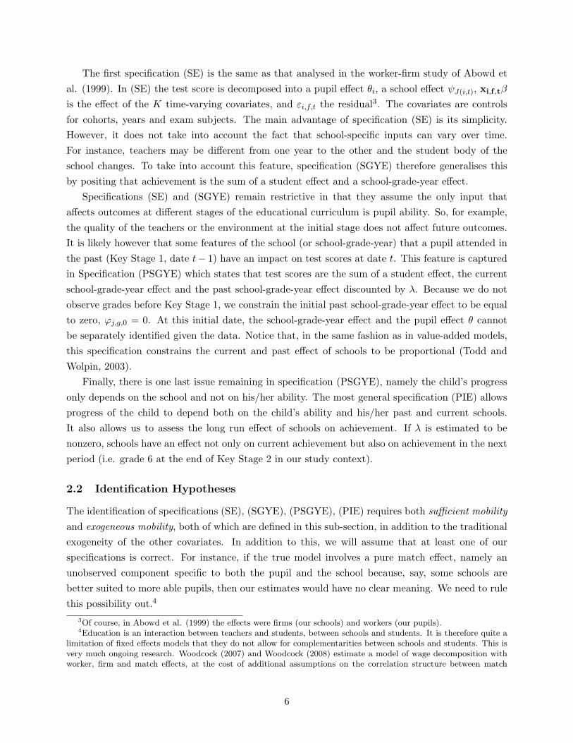
The first specification (SE) is the same as that analysed in the worker-firm study of Abowd etal. (1999). In (SE) the test score is decomposed into a pupil effect θi, a school effect ψJ(i,t), xi,f ,tβ

is the effect of the K time-varying covariates, and εi,f,t the residual3. The covariates are controlsfor cohorts, years and exam subjects. The main advantage of specification (SE) is its simplicity.However, it does not take into account the fact that school-specific inputs can vary over time.For instance, teachers may be different from one year to the other and the student body of theschool changes. To take into account this feature, specification (SGYE) therefore generalises thisby positing that achievement is the sum of a student effect and a school-grade-year effect.

Specifications (SE) and (SGYE) remain restrictive in that they assume the only input thataffects outcomes at different stages of the educational curriculum is pupil ability. So, for example,the quality of the teachers or the environment at the initial stage does not affect future outcomes.It is likely however that some features of the school (or school-grade-year) that a pupil attended inthe past (Key Stage 1, date t− 1) have an impact on test scores at date t. This feature is capturedin Specification (PSGYE) which states that test scores are the sum of a student effect, the currentschool-grade-year effect and the past school-grade-year effect discounted by λ. Because we do notobserve grades before Key Stage 1, we constrain the initial past school-grade-year effect to be equalto zero, ϕj,g,0 = 0. At this initial date, the school-grade-year effect and the pupil effect θ cannotbe separately identified given the data. Notice that, in the same fashion as in value-added models,this specification constrains the current and past effect of schools to be proportional (Todd andWolpin, 2003).

Finally, there is one last issue remaining in specification (PSGYE), namely the child’s progressonly depends on the school and not on his/her ability. The most general specification (PIE) allowsprogress of the child to depend both on the child’s ability and his/her past and current schools.It also allows us to assess the long run effect of schools on achievement. If λ is estimated to benonzero, schools have an effect not only on current achievement but also on achievement in the nextperiod (i.e. grade 6 at the end of Key Stage 2 in our study context).

2.2 Identification Hypotheses

The identification of specifications (SE), (SGYE), (PSGYE), (PIE) requires both sufficient mobilityand exogeneous mobility, both of which are defined in this sub-section, in addition to the traditionalexogeneity of the other covariates. In addition to this, we will assume that at least one of ourspecifications is correct. For instance, if the true model involves a pure match effect, namely anunobserved component specific to both the pupil and the school because, say, some schools arebetter suited to more able pupils, then our estimates would have no clear meaning. We need to rulethis possibility out.4

3Of course, in Abowd et al. (1999) the effects were firms (our schools) and workers (our pupils).4Education is an interaction between teachers and students, between schools and students. It is therefore quite a

limitation of fixed effects models that they do not allow for complementarities between schools and students. This isvery much ongoing research. Woodcock (2007) and Woodcock (2008) estimate a model of wage decomposition withworker, firm and match effects, at the cost of additional assumptions on the correlation structure between match

6

Notations: i, i′, i′′ are pupils. j, j′, j′′, j′′′ are schools or school-grade-years. Reading: i connects school j andschool j′ because i attends school j in the first period, and i attends school j′ in the second period.

Figure 1: (a) Sufficient mobility – The mobility graph has only one connex component. (b) Mobilityis not sufficient – The mobility graph has two connex components, {j, j′} and {j′′, j′′′}.

Mobility is defined as sufficient when the mobility graph for pupils and schools is connected(Abowd et al., 1999; Abowd, Creecy and Kramarz, 2002). Two schools are connected if and only ifat least one pupil has attended both schools in different years. The set of all these connections isthe mobility graph, and we say that it is connected when it has only one connex component. Thisis illustrated in figure 1.

Moreover, exogeneity assumptions specific to our model with pupil and school effects are re-quired (Abowd et al., 1999; Abowd et al., 2002). A threat to identification arises if, for instance,unmeasured unemployment shocks affect mobility and have an effect (e.g. through reduced income)on outcomes (Hanushek and Rivkin, 2003). For this example, assume those families who experiencean unemployment shock between the two periods are more likely (i) to make their child move toa bad school and (ii) to experience lower test scores due to their parents’ joblessness, then thedifference between bad and good schools might be underestimated.

To better understand why sufficient and exogenous mobility are jointly needed, consider the setof pupils who attend school j in period 1 and school j′ in period 2. This mobility is clearly necessarysince these movements allow the identification of the relative effectiveness of school j with respectto school j′. Ignoring the effect of covariates for the sake of clarity, this gives:

E[∆yi,f |i, J(i, 2) = j′, J(i, 1) = j] = ψj′ − ψj+ E[∆εi,f |i, J(i, 2) = j′, J(i, 1) = j] (1)

with ∆yi,f = yi,f,2 − yi,f,1 and ∆εi,f = εi,f,2 − εi,f,1. With exogenous mobility, E[∆εi,f |i, J(i, 2) =

effects and other fixed effects.

7

j′, J(i, 1) = j] = 0, the last term of the sum drops. This is potentially where unemployment shocks,divorce, etc. could make trouble. Exogenous mobility rules this possibility out. Now, given thisassumption, if ψj is identified then ψ′j is identified.

It is then easy to see that when the mobility graph has only one connex component, choosingone arbitrary school and one arbitrary pupil ı and setting their effects ψ and θı to zero identifiesall school and pupil effects. A formal definition of the mobility graph and the identification of themodel are detailed in appendix A.

So far our intuition has been built on the simplest specification SE. Introducing school-grade-year effects in specifications (SGYE) and (PSGYE) not only allows more flexibility in the measure-ment of school effectiveness, it also introduces more pupil mobility, since pupils necessarily changeyear-group between the two periods. In addition, because school-grade-year effects time-vary, theexogeneity assumptions are weaker than before. Model (SGYE) is a particular case of (PSGYE) inwhich the discounting factor is set to 0. Again, identification conditions are identical.

2.3 Identification of Peer Effects

Once we have estimated school-grade-year effects, we would also like to disentangle the effect ofthe social composition of the school-grade-year from the other inputs under plausible identifyingconditions. Identification of such peer effects is challenging. The main issues are described in Manski(1993). First, students may be sorted partly based on unobservable characteristics – for instance,teachers and students may not be randomly matched. Second, students influence each other whichmeans it is hard to disentangle the effect of one on the other; in other words, there is a simultaneitybias. And third, it is hard to identify the effect of peers’ characteristics from the effect of peers’behaviour.

We assume, as in Hoxby (2000a) and Gould et al. (2004), that the year-to-year variations inschool-grade-year composition are exogenous, essentially because of the randomness of the demo-graphics. For instance, in the case of ethnic peer effects, plus or minus one black caribbean studentin a given year is probably an idiosyncratic variation. We therefore regress the school-grade-yeareffect on a school identifier and the composition of the school-grade-year.

ϕj,g,t = ψj + E(z|j, g, t)γ + νj,g,t (2)

For each school-grade-year j, g, t, E(z|j, g, t) denotes the vector of average student characteristics,for instance the fraction of boys, the fraction of blacks, the fraction of free school meal students. Thisstrategy is likely to capture most of the bias due to non-random sorting of students between schools,essentially assuming that there is no correlation between changes in school-grade-year compositionand unobservable school inputs.

Formally, year-to-year variations in school-grade-year student composition should be exogenousconditional on the school-by-grade fixed effect. Variations in school-grade-year composition should

8

not be correlated with unobserved time-varying school characteristics.

E[νj,g,t=2 − νj,g,t=1|E(z|j, g, t = 2)− E(z|j, g, t = 1)] = 0 (3)

E(z|j, g, t = 2) − E(z|j, g, t = 1) is the year-to-year variation in school-grade-year composition.νj,g,t=2 − νj,g,t=1 represents unobserved time-varying shocks in school quality.

This hypothesis adresses the issue of the selection bias. The simultaneity bias is adressed throughthe use of a common school-grade-year effect for all students. Students “share” the same local publicgood, which includes peer-effects.

However we are not able to separately identify the effect of peers’ characteristics and the effectof peers’ behaviour. Thus the vector of social interactions γ captures both of these peer-effects.Thus in (6) γ is the reduced form peer-effect.

2.4 Decomposing Inequalities

The models we have specified allow us to decompose inequalities of test scores and test score gapsinto components attributed to schools, peers and pupils’ ability and background. We can do thissince test scores are the sum of the pupil effect, the year-group effect and the past year-group effect.In our KS2 and KS1 models, these can be written:

y2 = θ + ϕ2 + λϕ1 + ε2

y1 = θ + ϕ1 + ε1

where indices have been dropped for the sake of clarity. Moreover, school-grade-year effects can bedecomposed into a permanent school effect and the effect of school composition:

ϕ = ψ + zγ + ν

Inequalities of educational achievement can therefore be decomposed into inequalities of schoolquality, inequalities of pupil ability and background, and inequalities due to different social contexts,for instance stemming from varying patterns of segregation. In the first period:

V ar(y1) = Cov(y, θ) + Cov(y, ϕ1) + V ar(ε1)

The first term is the component due to pupils’ differences in ability and background. It is thesum of the heterogeneity in pupil ability and background, and the matching between pupil abilityand school-grade-year quality, i.e. Cov(y, θ) = V ar(θ) +Cov(θ, ϕ). The same decompositon appliesto school-grade-years, Cov(y, ϕ) = V ar(ϕ)+Cov(θ, ϕ). Hence, school-grade-year quality can wideninequalities in test scores if (i) school-grade-years are heterogeneous (ii) good pupils – high-θ pupils– are matched with good school-grade-years. Matching good school-grade-years to low-θ pupilsshould reduce inequalities.

9

This match between good school-grade-years and low-θ pupils can take two routes: (i) by fos-tering desegregation, i.e. decreasing Cov(γz, θ); and/or (ii) by matching high-ψ schools with low-θpupils.

2.5 Other Identification Methods Used in the Associated Literature

This section compares the identification strategy of this paper with the identification strategies thathave been introduced in past literature. We first compare our models to the value-added modelsthat are used in many papers on the measurement of school effectiveness. A seminal paper (Rivkinet al., 2005) uses this model to emphasize the importance of teacher effects on academic achievement.Finally, we compare the identification strategy of our paper to hierarchical linear models that haveflourished in the educational literature.

i) Value Added Models

In value added models, the outcome variable is the progress of the pupil rather than the absolutetest score. This basically corresponds to a dynamic panel data model in which the coefficient onthe lagged outcome is constrained to be equal to 1, i.e. λ = 1 in specification PIE. The results ofour estimations and of value added models are comparable.

A value added model would decompose the progress of the child into a child fixed effect, aschool-grade-year effect and a residual.

∆yi,f,t = xi,f ,t · β + θi + ϕJ(i,t),g(i,t),t + ui,f,t (4)

where ∆yi,f,t = yi,f,t − yi,f,t−1 is the progress of the child between two subsequent periods. Othernotations are as before. xi,f ,t is a vector of time-varying controls. There are two differences betweenthis model and specification PIE: (i) the value added model is more restrictive as it constrains theeffect of past achievement on current achievement so that λ = 1, and (ii) the error structure inthe value-added model is such that time varying unobservables can have long-term consequences onachievement. Indeed, the value-added specification can be rewritten as:

yi,f,t = xi,f ,tβ + xi,f ,t−1β + 2 · θi + ϕJ(i,t),g(i,t),t + ϕJ(i,t−1),g(i,t−1),t−1 + ui,f,t + ui,f,t−1 (5)

This model is equivalent to specification PIE when λ = 1 and ui,f,t + ui,f,t−1 = εi,f,t. Thus value-added models are equivalent to our model with a decay rate of 1, up to the error structure. Pointestimates should therefore be equal in both models. Our results reported below suggest that teachereffects are robust to a range of decay rates λ. Thus estimated effects from the value added modeland our full model should be similar.

10

ii) Teacher Effects: Rivkin et al. (2005)

Rivkin et al. (2005) specify an educational production function in which student value-added isdecomposed into a student effect, a school effect and a teacher effect. In our notation,

∆yi,f,t = θi + ψJ(i,t) + τT (i,f,t) + εi,f,t (6)

where ∆yi,f,t is the gain in student achievement of student i, in field f in year t. This specificationadds a teacher effect τT (i,f,t) where T (i, f, t) is the teacher of student i in field f in year t. In theirpaper, Rivkin et al do not identify all the effects, but rather use this specification as a blueprintand then estimate bounds for the variance of the teacher effects.

Specification (6) is remarkable in a number of ways. First, it does not include school-grade-yeareffects. Second, it includes teacher effects, which is an addition to specification (SE) of our paper.School effects ψJ(i,t) will not capture year-to-year variations of the student body, and the teachereffect τT (i,f,t) is likely to include both time-varying teacher quality and year-to-year variations ofthe student body that are correlated with changes in teacher quality.

iii) Metropolitan Area Fixed Effects: Hanushek and Rivkin (2003)

In Hanushek and Rivkin (2003), educational progress is decomposed into a family effect and ametropolitan area fixed effect.

∆yi,f,t = θi + θi,t +MSAM(i,t) + εi,f,t (7)

where ∆yi,f,t is the gain in student achievement of student i in topic f in year t. MSAM(i,t)

is a metropolitan area fixed effect, where M(i, t) is the metropolitan area of student i in year t.Estimation is carried out on Texas data, which contains 27 MSAs.

Three features of specification (7) are noticeable: first, student effects can vary over time;second, school effects nor school-grade-year effects are present; and last, metropolitan area fixedeffects do not vary over time. These elements have the following consequences. Student time-varying fixed effects are likely to capture other time varying inputs such as the metropolitan areasocial composition. Metropolitan area fixed effects are likely to capture public good quality andaverage school quality in the area, but not year-to-year variations of the social composition of thearea.

iv) Hierarchical Models for the Analysis of School Effects

Empirical work in education has used hierarchical linear models in several papers, notably in Rau-denbush and Bryk (1986), Bryk and Raudenbush (1992), Goldstein (2002) or Rao and Sinharay(2006). These models identify individual effects, school effects and potentially teacher effects usingonly cross-sectional data. Despite its light data requirements, an important limitation of multilevelmodelling is that they nest individual effects, school effects and other determinants of educational

11

achievement. Our model does not, since it uses pupil mobility to identify the effects. Multilevelmodels are written as a set of specifications at multiple levels, e.g. a student level equation and aschool level equation. Equations are then combined to lead to a single specification.

Another drawback is that Raudenbush and Bryk (1986) and Bryk and Raudenbush (1992) specifyrandom effects and not fixed effects. The identification of random effects require the assumption ofstrict exogeneity, which implies that, for instance, school effects are orthogonal to covariates and toother random and/or fixed effects (Wooldridge, 2002, p257). It is likely that, for instance studentswith a high or a low effect go to particular schools, or that schools with a good intake are particularschools. Thus it is unlikely that the orthogonality between the effects and covariates is a realisticassumption.

2.6 Estimation Method

The estimation of the model presented in this section cannot proceed in the same way as usualOrdinary Least Squares estimation techniques. The number of right-hand side variables is the sumJ − 1 +N +K of the number of school effects, pupil effects and the number of covariates.5 Usualpackages try to invert the matrix of covariates which is time consuming and numerically unstable.Abowd et al. (2002) have therefore developed an iterative estimation technique to estimate thebaseline fixed effects model of equation SE. However, specifications with past and current schoolor school-grade-year effects required new identification proofs and estimation techniques.

The estimation proceeds in the following way: first, it starts by computing the variance-covariance matrix of the model with dummies and covariates. This a large and sparse matrix.Second, starting with a first guess for fixed effects and coefficients – usually zero –, the procedureiterates by updating the approximate solution. The sequence of approximate solutions is obtainedby the conjugate gradient algorithm, that converges to the true solution if and only if the variancecovariance matrix is invertible; this requires that the mobility graph has one connex componentand that the covariates are linearly independent. More about the conjugate gradient can be foundin Dongarra, Duff, Sorensen and van der Vorst (1991). Details of the computation of the variance-covariance matrix are given in Appendix B and these computation techniques have given birth toa set of programs developed by the authors and are freely available on the website of the CornellInstitute for Social and Economic Research.

3 Dataset and Estimation Method

3.1 The English Educational Context

The English educational system currently combines market mechanisms (many of which were in-troduced in the Education Act of 1988) in different types of schools with a centralized assessmentoperating through a National Curriculum (Machin and Vignoles, 2005). Therefore it has the ad-

5One school or school-grade-year effect is set to zero, one pupil effect is set to zero, and we add a constant.

12

vantage of providing us with fairly different management and funding structures and, at the sametime, national exam results for all students.

The assessment system features a National Curriculum which sets out a sequence of Key Stagesthrough the years of compulsory schooling: in primary school Key Stage 1 (from ages 5 to 7) andKey Stage 2 (from ages 7 to 11); and in secondary school Key Stage 3 (from ages 11 to 14) andKey Stage 4 (from ages 14 to 16). At the end of each Key Stage, pupils are assessed in the coredisciplines: Mathematics, English and Science (not for Key Stage 1). These tests are nationally setand anonymously marked by external graders.

The English primary schooling system is also characterised by a variety of different managementstructures and funding sources. Community schools and voluntarily controlled schools, which caterfor more than half of the student body, are controlled by the Local Education Authority (LEA),of which there are 150 in England. In the case of community and voluntarily controlled schools,the LEA owns the buildings and employs the staff. On the other hand, in voluntary aided andfoundation schools, teachers are employed by the school governing body and the LEA has no legalright to attend proceedings concerning the dismissal or appointment of staff.6 Funding also variesacross school types. While most state schools are funded by the government, voluntary aided schoolscontribute around 10% of the total capital expenditure. These management and funding differencesare likely to generate various kinds of incentives, and thus different educational outcomes for pupils.

3.2 The National Pupil Database

The National Pupil Database (NPD) is a comprehensive administrative register of all English pupilsin state schools. Data is collected by the Department for Children, Schools and Families and it ismandatory for all state schools to provide accurate data on pupils, who are followed from year toyear through a Pupil Matching Reference. Thus panel data can be built by stacking consecutiveyears of the National Pupil Database.

The dataset provides rich information on pupils’ characteristics: gender, free school meal status,special educational needs, and the ethnicity group. Pupils who receive free meals are the 15 to20% poorest pupils. The ethnicity variable of our sample encodes the main ethnic groups: White,Black Caribbean, Other Black, Pakistani, African Black, Mixed background, Bangladeshi, Indian,Chinese, Other Background.7 It also provides some information on school structures and types (i.e.whether they are community schools, foundation schools, voluntary aided or voluntary controlledschools, and so forth).

Test scores in English, Maths and Science are available - the latter Science test only for KeyStage 2. These tests are externally set and marked. We have standardized test scores to a mean of50 and a standard deviation of 10 to make results comparable from one level to the other and fromyear to year.

The structure of the panel data we have built from the NPD is shown in Table 1.6Code of Practice on LEA Schools Relationships, DfES 20017Coding of the ethnicity variable has changed in the period we consider. It was therefore necessary to recode it in

a time-consistent manner.

13

4 Main Results

We now come to the policy questions of the introduction: do schools matter? do peers matter? aredifferent schooling structures important?

4.1 Pupil, School and School-Grade-Year Effects

Do schools matter? Over the years, this question has been extensively discussed in the sociologicaland educational literature as well as in recent papers in the economics of education (Rivkin et al.,2005). Our new method of estimating school-grade-year effects and individual effects specificationsgives us a new opportunity to re-assess this important question, based upon the extremely richEnglish data we study.

The estimation of specifications SE to PIE yields pupil fixed effects, school-grade-year effectsand school effects. School-grade-year effects are not available for the simple school effects model(specification SE). Some very clear stylized facts come out from considering the correlations andvariances/covariances reported in Tables 4 and 5: (i) first of all, pupils are much more heterogenousthan either school or school-grade-years effects (ii) individual effects explain a much larger share ofthe variance of test scores than school or school-grade-year effects.

The first key finding is of a higher variation of pupil fixed effects as compared to school-grade-yeareffects and school effects can be seen from the Tables, where the standard deviation of pupil effectsis between 3.8 and 4.8 times larger than the standard deviation of school effects. Thus, perhapsnot surprisingly, suggests that pupils are more heterogeneous than schools. The same finding, ofa higher variation, is also true when comparing the standard deviation of pupil effects and thestandard deviation of school-grade-year effects. Nevertheless, pupil fixed effects are less preciselyestimated than school-grade-year effects or school effects. Indeed, at most five observations perchild are available whereas on average 250 observations per school-grade-year are available. Toaddress this potential issue, we look at the correlation between test scores and the school or school-grade-year effects. Individual effects are imprecisely estimated but this should actually lower thecorrelation between individual effects and test scores.8

The correlation between test scores and individual effects is seen to be between 0.79 and 0.83.This is between 5 and 6.7 times larger than the correlation between school effects and test scores.Indeed, the covariance Table 5 confirms the explanatory power of pupil effects to be much largerthan the explanatory power of school effects. This is no surprise given the high correlation, the lowvariance of school effects and the much higher pupil heterogeneity.

Therefore these baseline results strongly suggest that pupil effects are a more important de-terminant of test scores than school effects. How can one interpret these pupil effects? From ourperspective, it seems reasonable to think of them as picking up the whole range of educational ex-periences before age 7: this includes parental background, childcare and kindergarten. Consideredin this way, the fact that pupil effects explain most of the variance of test scores is in line with some

8This, of course, holds provided measurement error is classical.

14

of the important contributions to the recent economics of education research area (including, interalia, Heckman and Masterov (2007), Currie (2001) and Garces, Thomas and Currie (2002)).

4.2 Pupil Effects: Disentangling Individual Effects From Peer Effects and School

Quality

Of course, pupil effects can be correlated with a range of individual characteristics (like ethnicity,gender, free school meal status, special needs and the child’s month of birth) and so an importantresearch challenge is to try to disentangle them from other factors like peer effects and school quality.Doing so differs from an analysis of raw test scores since, under maintained assumptions, it looksat pupil effects free of peer effects and free of the correlation between school quality and observablecharacteristics.

From our analysis it is evident that pupil effects are reasonably well explained by observablecharacteristics. For example, the R-Squared from regressions of the fixed effects on observable char-acteristics is around 40% (Table 6). In these regressions, the estimated coefficients are remarkablyrobust to different specifications. Moreover, the results are in line with descriptive statistics on testscores. The pupil fixed effects of free school meal children are 40 to 41% of a standard deviationlower. Family disadvantage is important, with free school meal pupils being the 10 to 20% poorestchildren in England. Chinese pupils are the best performing pupils, with a fixed effect 16% of astandard deviation higher than white pupils. Interestingly, Indian pupils have a lower fixed effectthan white pupils (6.4 to 7.8% of a standard deviation lower), whereas the test scores of Indianpupils are higher than the test scores of whites. This suggests that basic descriptive statistics donot disentangle the effect of ethnicity from the effect of peers and the effect of school quality. Finally,male pupils have a higher fixed effect, by 2.5 to 2.6% of a standard deviation. This is certainly due tothe fact that regressions were carried out by pooling all subjects together. Boys in primary schoolare better at mathematics and science, whereas girls are better at English. There are thereforearound three observations for which boys are better – maths in grades 2 and 6, science in grade 6– and 2 observations for which girls are better – English in grades 2 and 69.

Table 6 confirms that pupil effects are well explained by observable characteristics, even if oneis unable to offer a causal interpretation to the reported findings. The coefficients in Table 6 proveto be very consistent with basic descriptive statistics and, at the margin, this analysis allows us todisentangle pure individual effects from the social context working through peers and school quality.

4.3 Effects of Social Composition on School Quality

As discussed in Section 2.3, the effect of the gender, ethnic and social composition of the school on itsquality can be identified under the assumption that year-to-year variations in school composition areexogenous(Hoxby, 2000a; Hoxby, 2000b; Lavy and Schlosser, 2007). Two stylized facts emerge fromthe covariances in Table 5 and from regressions of school-grade-year effects on school composition

9Another version of the tables, available upon request, discarded science test scores. Male fixed effects are thennot significantly higher.

15

and school effects reported in Table 7: (i) the covariance between school-grade-year effects and testscores is comparable to the covariance between school effects and test scores; and (ii) some of thepeer effects are significant but small – effect of the fraction of boys, free meals and special needs.Overall, results suggest peer effects to be statistically significant, but relatively small in magnitude.

Looking at the covariances in Table 5 shows the covariance between test scores and schooleffects to be very similar to the covariance between test scores and school-grade-year effects; 5.6 vs.7.7 for the school-grade-year specification, 4.6 vs. 4.2 for the past and current school-grade-yearspecification, and 4.7 vs. 4.0 for the full-fledged specification. Since school-grade-year effects canbe decomposed into the school effect and the effect of social composition, these figures imply thatpeer effects are likely to be less important than school quality.

Table 7 shows estimates of the effect of the fraction of different social groups on school-grade-yeareffects, separately for grade 2 and grade 6. In grade 2, in the full-fledged specification, increasingthe fraction of male students by 10% makes school-grade-year effects fall by 0.4% of a standarddeviation10 (Table 7, column 3). This effect is robust to different specifications. In grade 6, theeffect of the fraction of boys is positive, i.e. increasing the fraction of boys by 10 percentage pointsincreases test scores by 0.9% of a standard deviation (Table 7, column 6). The difference betweengrade 2 and grade 6 gender composition effects is likely to be due to the fact that grade 2 examsare in English and Maths, whereas grade 6 exams are in English, Maths and Sciences. Boys arebetter than girls in both science and maths, but not better in English. This effect is robust to theinclusion of past school-grade-year effects and past individual effects in the baseline specification.Most papers in the literature find a negative effect of boys on achievement both in English and inMaths, e.g. Hoxby (2000a).

The fraction of free meal children has a detrimental effect on school-grade-year effects in grade6; increasing the fraction of free meal children by 10 percentage points lowers school-grade-yeareffects by 0.7% of a standard deviation (Table 7, column 6).

In grade 6, ethnic composition has an effect on school quality. Chinese and Indian children exerta positive contextual effect, black caribbean children exert a negative contextual effect. The effectsare large: increasing the fraction of chinese students by 10 percentage points increases fixed effectsby 4.6% of a standard deviation (table 7, column 6). These results are in line with the intuitionthat being surrounded by high performing peers is good for your test scores; chinese children are atthe top of the test score distribution, and black caribbean children are at the lower tail.

Special needs pupils have a negative impact on achievement under the identification assumption.Indeed, increasing the fraction of special needs students by 10% decreases school-grade-year effectsby 6% of a standard deviation. Other effects are not significant in grade 2. The contextual effect ofspecial needs students includes both the direct effect of interacting with special needs students andthe effect that goes through teachers’ and principals’ behaviour (Todd and Wolpin, 2003). Section5 will look more closely at probing the identification assumptions.

10The standard deviation of test scores is 10.

16

4.4 School Quality and School Structures

Are some schools better than other schools? Are schools that are organised under particular struc-tures better than others? This is an important question, even if school quality explains a smallshare of the variance of test scores, since there may be scope for improvement in the way schools arestructured. As has already been noted, English schools can have a variety of different organizationalstructures. Some schools are able to hire and dismiss their staff, while in other schools the staff isrecruited and dismissed by the Local Education Authority (table 3).

The regressions shown in Table 8 do indeed show significant differences by school type. Thereis evidence of beneficial effects of local recruitment of staff coupled with external control of theschool board. Indeed, in both grade 2 and grade 6, voluntary controlled schools perform worse thancommunity schools; like community schools, they cannot locally manage their human resources anddo not own their assets. The main difference with community schools is that they are mostly Churchof England schools.

Table 8 shows that voluntary aided schools, who can hire and dismiss staff locally, have a higherschool fixed effect in grade 6, by 3 to 4 % of a standard deviation. The effect is not significant ingrade 2 (table 8). Other types of schools can hire locally, e.g. foundation schools. These schools donot have a significantly higher school effect in grade 2 and grade 6. But the board of foundationschools is controlled by the Local Education Authority, whereas the board of voluntary controlledschools is mostly controlled by the foundation. Broadly speaking, schools with a high fixed effectrecruit locally and the majority of their board is externally controlled by their foundation.

School management structures are not the whole story, though. The R-Squared of the regressionsof school effects on school type dummies is small, being not more than 1%, a finding in line withthe school effectiveness literature we cited earlier. There are therefore many other determinants ofschool quality that, unfortunately, are not observed in the dataset we utilise.

4.5 Longer Run Effects of School Quality and Peers

Specifications PSGYE and PIE allow for some persistence of the effect of school quality, since pastschool-grade-year effects are included in the determinants of test scores. In specification PIE, weallow for a potential effect of the pupil’s background on the progress of the child. The discountingfactor therefore measures the long term effect of school quality and of pupil background on progress.These two features matter as long as λ is nonzero.

λ is estimated by minimizing the sum of squared residuals. In specification PSGYE, whichinclude past school-grade-year effects, the decay rate λ is imprecisely estimated. Table 9 showsthe sum of squared residuals for a range of λs, from 0 to 0.9. For the 1998-2002 cohort and the2000-2004 cohort, the optimal discounting factor is zero.11 For the cohort in-between, the optimaldiscounting factor is 0.1. But a likelihood ratio test and its associated χ2 statistic reveal that it isnot possible to reject the hypothesis that λ is different from any value between 0 and 0.912. The

11Due to the large number of computations, we decided to estimate λ at a precision greater than 1/10.12Under the null hypothesis that λ is equal to the optimal lambda, e.g. λ∗ = 0, the statistic 2 · ln(L(λ)/L(λ∗))

17

good news though is that the school-grade-year effects and the pupil effects are robust to smallvariations of λ around zero.13

The discounting factor is much more precisely estimated in the last specification (table 9). Theoptimal discounting factor is 0 for the 1998-1999 cohort, 0.1 for the 1999-2000 cohort and 0 for the2000-2004 cohort. Results indicate that on the whole the school-grade-year effect and individualeffect specification (equation PSGYE) is not rejected and fits the data as well as the last twospecifications. This is evidence that school quality and peer effects may have little long run effects.This is consistent with Hanushek (2003) and with the notion that, for instance, reductions of classsize have small long term effects (Prais, 1996; Krueger, 1999). Similarly, Angrist and Lang (2002)suggest that peer effects in the Boston METCO program were short-lived.

4.6 Pupil Mobility

Table 10 offers an analysis of patterns of pupil mobility. At this stage, it does not aim at checkingwhether the identification assumptions required in our analysis are supported by the data. Rather,that analysis is deferred to the next section of the paper. Instead, at this juncture, we wish toprovide some stylized facts about pupil mobility in English schools using the estimates of schooland pupil effects.

The table shows two main patterns worthy of discussion. First of all, pupil mobility in primaryschool seems on the whole to be a feature of low performing pupils from low quality schools. Pupileffects are negatively correlated with next period school effects and school-grade-year effects. In-creasing the pupil effect by 10% of a standard deviation reduces the probability of moving by 0.3%.And increasing the pupil effect by 10% of a standard deviation is correlated with a 0.5 % fall of thenext period school-grade-year and a 0.2% fall of the next period school effect. Free school mealsare more likely to move (line 5 of table 10). They also move to particular schools, i.e. other schoolsthan most pupils from their school. They move to lower quality school-grade-years (column 3). Onthe other hand, they move to schools with a higher school fixed effect. This means that they tendto go to schools with a worst peer group but better school quality.

The second main result is that disadvantaged ethnic backgrounds tend to move less than whitechildren and movers from these ethnic backgrounds tend to go to better schools than white chil-dren. Bangladeshi pupils are 11.4% less likely to move than white children. Pakistani pupils are6.8% less likely to move than white children and black caribbean children are 5.4% less likely tomove. Bangladeshi especially tend to go to better schools, next period school-grade-year effects arehigher by 15% of a standard deviation, school effects are higher by 12% of a standard deviation,conditionally on the school effect and school-grade-year effect of grade 2.

converges to a χ2 statistic (Hoel, 1962).13Results available on request.

18

5 Robustness Checks and Further Discussion

In this section, we check present a number of robustness checks of our main finding, in particularfocussing on whether our identification assumptions are supported by the data. The identificationof school quality assumes at least sufficient mobility and exogenous mobility. The identification ofpeer effects moreover assumes that year-to-year variations in cohort composition are exogenous. Wediscuss these assumptions in the following subsections.

5.1 Do Children Move Enough to Generate Identification of the Model?

To separately identify pupil effects from school or school-grade-year effects, pupils have to movebetween schools. More precisely the mobility graph as defined in section 2.2 should have oneconnex component. Table 11 presents some basic statistics on mobility. Most pupils are followedfrom Key Stage 1 to Key Stage 2. A sizeable proportion (42%) of pupils also change school betweengrade 2 and grade 6. This is sufficient to generate only one mobility graph. The empirical questionof importance of whether students who move are actually different from pupils who do not move isaddressed in the following section.

5.2 Is Mobility Endogenous?

School quality and the effect of pupil background on achievement are estimated by comparing pupils’test scores in different schools. It therefore requires that pupil mobility is not driven by unobservedshocks that affect test scores, such as divorce, unemployment, and other family events. We arguein this section that there is a credibly exogenous source of mobility. Indeed, some primary schoolsonly cater for key stage 1 pupils. Mobility is compulsory in this case. It proves important thatwhen the model is estimated on compulsory movers only, this paper’s results are not significantlyaffected.

i) Why Endogenous Mobility may be a Problem

We design a small, simple model to understand why endogenous mobility may be a problem. In thismodel, households experience unemployment shocks that are unobserved by the econometrician.When a household experiences an unemployment shock, children change school and their test scoresare likely be lower.

The model is set up as follows. There are two periods. In each period, pupils’ parents can eitherbe unemployed ui,t = 1, or employed ui,t = 0. Test scores are determined by the following equation:

yi,t = θi + ψJ(i,t) − δui,t + ηi,t (8)

(8) is a school effect model. We restrict ourselves to a model with school effects for expositionalease. yi,t is the test score of pupil i in year t. ψj is the school effect of school j. δ is the adverse

19

effect of unemployment on test scores, and ui,t is a dummy for unemployment. ηi,t is a residual.Unemployment shocks ui,t, i = 1, 2, t = 1, 2, are unobserved and the econometrician estimates

the following specification:

yi,t = θi + ψJ(i,t) + εi,t (9)

Assuming exogenous mobility, the estimated school effects ψj are estimated by OLS. To under-stand the relationship between the structural effects and the least squares estimates, let us writethe specification in matrix form.

Y = Dθ + Fψ − δU + ε

with Y the vector of test scores, D the design matrix for pupil effects, θ the vector of pupil effects,F the design matrix for school effects, ψ the vector of school effects, U the vector of unemploymentshocks and ε the residual.

The estimates are as follows:

θ = θ − δ(D′MFD)−1D′MFU (10)

ψ = ψ − δ(F ′MDF )−1F ′MDU (11)

where MD is the matrix that projects a vector on the vector space that is orthogonal to D. Thesame logic applies to MF .

Thus the estimates of the individual effects and the school effects are biased whenever thecorrelation between unemployment shocks and design matrices F or D is nonzero, that is, whenevermobility is endogenous. When unobserved unemployment shocks (i) drive pupils to particularschools and (ii) affect their test scores, the estimates of school effects and pupil effects are biased.

ii) Compulsory Moves as an Exogenous Driving Force of Mobility

Compulsory movers are children who move between grade 2 and grade 6 because their key stage 1school does not cater for key stage 2 children. This mobility is likely to be more exogenous thanvoluntary moves. However, there are three important conditions: (i) compulsory movers should notbe significantly different from non compulsory movers; (ii) as compulsory mobility is expected byparents, we need to get evidence that key stage 1 only schools are not particular schools – eitherbetter or worse schools; (iii) compulsory mobility provides us with a exogenous reason to move, butit does not per se give an exogenous direction of mobility; children may still sort endogenously intoschools.

Table 12 shows descriptive statistics for compulsory movers, noncompulsory movers and stayers.Genders, months of birth, languages and ethnicities are very similar between compulsory movers,noncompulsory movers and stayers. Differences between the three categories appear in the fraction

20

of special needs students and free school meals. The fraction of free school meal students is higheramong noncompuslory movers than among compulsory movers, but it very similar between com-pulsory movers and stayers. On the whole, there are slight differences between the three categoriesof mobility.

We therefore performed the estimation of specifications SE and PSGYE on compulsory moversonly14. Correlation tables (table 14) reveal that stylized facts are robust to the exclusion of noncom-pulsory movers: (i) pupil heterogeneity is bigger than school heterogeneity and school-grade-yearheterogeneity (ii) the correlation between test scores and individual effects is bigger than the corre-lation between test scores and either school effects or school-grade-year effects.

Pupil heterogeneity is similar in table 4 and in table 14. School-grade-year or school hetero-geneity, while still smaller than pupil heterogeneity, is bigger in the school effects specification withcompulsory movers only (6.938 vs 1.941). This might be due to the smaller number of observa-tions in the estimation with compulsory movers only. School effects heterogeneity is comparable inthe school-grade-year specification with and without noncompulsory movers. Stylized facts do notchange when estimating regressions with compulsory movers only.

The last issue we need to address is whether the direction of mobility is likely to be an iden-tification issue. We define the most frequent school pupils go to. For each school j, the numberof pupils who move from school j to school j′ is computed. The most frequent school pupils fromschool j go to in the next period is noted M(j). Among pupils who move, 63% move to the mostfrequent school (table 11). This is mainly made up of compulsory movers. Therefore compulsorymovers mainly tend to go to the ’usual’ school, and the direction of their mobility is not likely tobe mainly explained by individual unobserved time varying variables.

5.3 The Identification of Peer Effects: Are Year-to-Year Variations in Grade

Composition Exogenous?

The effect of grade composition on school quality is estimated by looking at how year-to-yearvariations affect school-grade-year effects. This actually requires that year-to-year variations ingrade composition are not correlated with other changes in school inputs, such as changes in teacherquality and school funding. One way of addressing this identification issue is to compare year-to-yearvariations to truly random variations around school average composition.

Formally, if changes in grade composition are truly exogenous, they must be some random fluc-tuation around the average school composition. In a way identification relies on the idea that gradecomposition in a given year is a finite size approximation of the school’s equilibrium composition.

E(z|j, g, t) = E(z|j, g) + uj,g,t (12)

Notations as before. E(z|j, g, t) is the empirical school-grade-year composition in school j, grade gand year t. This is a vector containing the percentage of each ethnicity, the percentage of boys, free

14We also performed the estimations of the two other specifications, yielding similar results.

21

meals and special needs. E(z|j, g) is average school composition across the three cohorts. The sizeof the noise is approximately normal with variance around V ar E(z|j, g)/√nj,g,t.

The dataset only contains the empirical composition of grades. Therefore school average com-position is just an estimate of the true composition.

E(z|j, g) = E(z|j, g) + vj,g,t (13)

with the size of the error term approximately V ar E(z|j, g)/√nj,g. Therefore, finally, E(z|j, g, t) =E(z|j, g) + uj,g,t − vj,g,t.

Figure 2 compares the results of simulations to actual year-to-year variations in school-grade-yearcompositions. For boys, free meals and three important ethnic groups year-to-year variations areremarkably similar to random variations, as in Lavy and Schlosser (2007). This suggest that trendsin school-grade-year composition are not likely to explain the results of peer effects regression. Onthe other hand, year-to-year varations in the fraction of special needs is bigger in the dataset thanwhat would be expected if it were purely random. There may be trends in the fraction of specialneeds students in schools, which is likely to be due to evolving support for special needs studentsin English elementary schools. Broadly speaking, apart from special needs students, variations ingender and ethnic compositions are similar to random variations around average school composition.

5.4 What Can League Tables Tell Us?

The Education Reform Act 1988 set up the National Curriculum, which follows pupils through keystages, as we pointed out in section 3.1. Since the early 1990s league tables have been publiclyavailable in England - for example, measures of performance at the end of each key stage arenow disclosed on the BBC’s website and through local newspapers. This is a crucial element oftransparency that is coupled with some leeway for school choice. Parents typically submit theirfirst three choices to Local Education Authorities in the fall of the academic year before enrollment;most faith schools require a special application form.

Measures of performance are published in league tables. These league tables have becomeincreasingly more sophisticated over time. They currently reveal three pieces of information: (i) theaverage test score at key stage examinations; (ii) the average value added of pupils in the school;value added is the difference between the pupil’s test score in the previous key stage and his currenttest score; finally, (iii) the average test score and value added in the local authority.

Are these elements informative about school effectiveness? The answer depends on the shape ofthe education production function. It turns out that, using our models, neither absolute test scoresnor value added measures are good estimates of school effectiveness ϕ or ψ. In the full-fledgedmodel with non-zero decay rate and past inputs, the average test score of a school is a mixture ofschool effectiveness, the average individual effect in the school and the average effectiveness of pastschools. Indeed,

22

E[yi,f,t|j, g = 6, t] = (1 + λ) · E[θi|j, g = 6, t] + ϕj,g=6,t + λ · E[ϕj,g=2,t−4|j, g = 2, t− 4] (14)

where notations are as before. t is the year, g = 6 says that we are considering test scores ingrade 6. E[yi,f,2|j, g = 6, t] is the average test score in school j, grade g in grade 6. In two of thethree cohorts, the estimated decay rate is not different from zero. In this case, average past schooleffectiveness disappears but the average individual effect remains. Therefore, unless two schoolshave the same intake, the average test score is not informative about ϕ. Presumably this mattersfor issues of school accountability.

How important is the contribution of individual fixed effects to school average test scores? Table15 shows the decomposition of the between-school variance of test scores into its components. Mostof the variance of pupil effects is within schools (76%). There is however substantial between-schoolvariance of the pupil effects (24% of the variance of pupil effects). More troubling, the between-school variance of individual effects is very close to the between-school variance of test scores.This suggests that average test scores are a flawed measure of school effectiveness, provided ourspecification is correct.

Value added measures are a means to get rid of these confounding effects. Average value addedis:

E[∆yi,f |j, g = 6, t] = λ · E[θi|j, g = 6, t] + ϕj,g=6,t + (λ− 1) · E[ϕj,g=2,t−4|j, g = 2, t− 4] (15)

where ∆yi,f = yi,f,2 − yi,f,1. E[∆yi,f |j, t] is average value added in school j, in a given year t.Again, λ is close to zero in most cohorts, so that average value added is free of the individualeffects. However, average past school quality still enters the equation. It is a priori a problem sincethe variance of school effects in grade 2 is comparable to the variance of school effects in grade 6.

Overall, neither average test scores nor average value added measures are a good proxy for schooleffectiveness. It seems that more elaborate statistics are needed to truly help parents in accuratelydetermining their school choice decisions. The findings of our paper suggest that an index whichdoes not conflate pupil, school and peer effects and one that does not relate on value added couldbe superior. Of course, there is a trade-off between the complexity of our approach to generatemeasures and the ’simpler’ measures currently reported, but the estimates of school effects fromour approach can be calibrated into the information set of those with an interest in which schoolsgenerate better performance for children.

Moreover, school effects are precisely estimated: the difference between the 60th percentileschool effect and the 40th percentile school effect is significant in all specifications, with a standarderror suggesting that our estimates could be used to differentiate school quality up to a percentilepoint.15 This is in stark contrast with Chay, McEwan and Urquiola (2005) and Bird, Cox, Farewell,

15Bootstrap was performed to compute the standard error of the statistic ψP60 − ψP40. Block bootstrapping was

23

Goldstein, Holt and Smith (2005), which find that average test scores and value-added are essentiallynoisy measures.

5.5 Matching of Pupils to Schools

Results have shown that the most relevant specification is equation PSGYE. In this specification,schools are equally effective for all students, that is, there is no complementarity between pupilsand schools. If the educational production function is truly specified as in specification PSGYE, themodel does not predict any particular matching of pupil effects and school effects at equilibrium.Matching patterns are indeed determined by the complementarity between pupil effects and schooleffects, following Becker (1973)16. In such a world, the model predicts zero correlation betweenpupil effects and school-grade-year fixed effects.

However, some of the correlations between child effects and school effects in table 4 are negative.Does it mean that pupils with a high pupil effect are structurally matched with low school-grade-year effects? The correlation between estimated pupil effects and estimated school effects is actuallydownward biased and we perform simulations to estimate the magnitude of the bias, suggesting thatthe correlation is likely to be close to zero.

The correlation between estimated effects is downward biased. This has been pointed out in thecontext of worker-firm matched panel datasets (Abowd and Kramarz, 2004). To make this clear, letus decompose the correlation between child and school effects. This correlation can be written asthe sum of the correlation between measurement errors and the true covariance between the effects.

Cov(θ, ϕ) = Cov(θ − θ, ϕ− ϕ) + Cov(θ − θ, ϕ) + Cov(ϕ− ϕ, θ) + Cov(θ, ϕ)

where θ is the individual effect, ϕ is the school-grade-year effect, θ is the estimated individual effect,ϕ is the estimated school-grade-year effect.

The estimation of Cov(θ, ϕ) therefore requires the estimation of Cov(θ − θ, ϕ), Cov(ϕ, θ − θ),Cov(θ − θ, ϕ − ϕ). In general, the measurement errors of child and school effects are negativelycorrelated (Abowd and Kramarz, 2004). The intuition behind this result is that (i) pupils whochange school get a better estimated effect but school effects are less precisely estimated (ii) pupilswho do not change school have a less well estimated effect but their associated school effect is moreprecisely estimated.

Simulations can assess the order of magnitude of the downward bias of the correlation. Wegenerate pupil effects who have a normal distribution with the same variance as the estimated pupileffects. We also generate school effects the same way. The point here is that pupil effects and schooleffects are uncorrelated. We then generate simulated test scores using the specification with pastand current school-grade-year and individual effects.

used, with little difference on the size of standard errors. The difference ψP60 − ψP40 was 1.12 with a standard errorof 0.057 in specification SGYE.

16This of course, assumes a particular form of preferences and special market conditions. The housing market shouldbe perfect, parents should know the educational production function as specified in equation PSGYE and the onlyreason for location decisions should be the level of test scores.

24

Results are presented in table 16. Simulated pupil effects and school-grade-year effects weregenerated using the variances of the last table of table 4. The results of simulations suggest thateven in the absence of a true correlation between pupil effects and school effects, the correlationbetween estimated effects is negative. The correlation is −0.033. The empirical correlation is stableacross the three simulations. The correlation between school-grade-year and individual effects istherefore likely to be close to −0.1, with school-grade-year effects explaining little of the varianceof test scores.

Generally speaking, estimating the correlation between pupil effects and school effects remainsa difficult challenge in pupil-school or worker-firm fixed effects specifications. Most papers find azero or negative correlation (Abowd and Kramarz, 2004; Abowd et al., 1999). But these papers donot include a match effect that could account for the complementarity between pupil and school-grade-year effects or worker and firm effect. The identification proofs of appendix A are not validin this case and more stringent identification assumptions are needed (Woodcock, 2007).

6 Conclusion

In this paper we consider a detailed econometric model which evaluates the importance of pupiland school factors in determining children’s educational achievement. There are some parallels withthe by now large literature that estimates worker and firm effects from data matching workers tofirms. Here we match pupils to schools, using very rich adminstrative data on English primaryschool children. We develop a set of econometric techniques that allow us to decompose childrens’test scores into the effect of the background, the effect of the peers and the effect of the schools.This is identified under general conditions of sufficient and exogenous mobility.

The main finding from this detailed econometric model is that pupil ability and background isprobably the most important educational input in that it explains a large fraction of the overallvariance. This suggests that either inherited ability, early educational experiences (acquired beforethe age of seven) and family background play a very important part in the educational process.School time-invariant inputs are the second most important input, but prove to be far less importantthan pupil effects, provided the identification and specification of our models is correct. Peereffects may be the least important input, most effects being small. The analysis of mobility revealsthat a substantial fraction of mobility is due to the structure of the English schools system wherecompulsory mobility occurs at certain stages. This provides us with a reasonably exogenous sourceof mobility. Results reveal that high achieving pupils either tend to stay in the same school, or togo to the most usual school which students go to.

The findings of this paper should be useful to a number of audiences and research areas. First ofall, they do have clear implications for education policy and design. It is evident that pupil-specificfactors matter most, a conclusion also reached in other areas of the social sciences, through verydifferent modelling approaches (e.g. the ’school effectiveness’ literature in education research). Thisthrows doubt on the relevance of many simple measures of school effectiveness published on the

25

internet and in local newspapers in many countries. Second, this paper applies and refines methodsfrom the literature on matched worker-firm data to pupils in schools. We think this is important,providing strong evidence showing how economic agents (in this case pupils) behave and adapt inthe environment (in this case schools) in which they spend a considerable amount of their time.It is very clear from our analysis (and from related ones like Rivkin et al. (2005)) that one gainsa lot from observing pupils in the schools they attend and we can say a lot more than a studyof educational achievement based only on pupils or only on schools is able to. Thirdly, and moregenerally speaking, this paper estimates a full-blown specification with semi-parametric estimatesof pupil background effects, peer effects and school effects. It is the first paper of this kind toinclude peer-effects and to include the effect of past schools(-grade-year) as current inputs. Theseconclusions may be of substantial interest to policy makers seeking to spend public funding into theright inputs either to increase efficiency or to narrow educational inequalities.

References

Abowd, J., Creecy, R. and Kramarz, F. (2002), Computing person and firm effects using linkedlongitudinal employer-employee dataset, Technical report, US Census Bureau.

Abowd, J. M. and Kramarz, F. (2004), Are good workers employed by good firms? A simple testof positive assortative matching models, Econometric Society 2004 North American WinterMeetings 385, Econometric Society.

Abowd, J. M., Kramarz, F. and Margolis, D. N. (1999), ‘High wage workers and high wage firms’,Econometrica 67(2), 251–334.

Angrist, J. D. and Lang, K. (2002), How important are classroom peer effects? Evidence fromBoston’s METCO program, NBER Working Papers 9263, National Bureau of Economic Re-search, Inc.

Becker, G. S. (1973), ‘A theory of marriage: Part I’, Journal of Political Economy 81(4), 813–46.

Bird, S. M., Cox, D., Farewell, V. T., Goldstein, H., Holt, T. and Smith, P. C. (2005), ‘Performanceindicators: Good, bad, and ugly’, Journal of the Royal Statistical Society 168(1), 1–27.

Blundell, R. and Robin, J. M. (1999), ‘Estimation in large and disaggregated demand systems: anestimator for conditionally linear systems’, Journal of Applied Econometrics 14(3), 209–32.

Bryk, A. and Raudenbush, S. (1992), Hierarchical Linear Models: Applications and Data AnalysisMethods, Sage, Newbury Park.

Chay, K. Y., McEwan, P. J. and Urquiola, M. (2005), ‘The central role of noise in evaluatinginterventions that use test scores to rank schools’, American Economic Review 95(4), 1237–1258.

26

Clotfelter, C. (1999), Are whites still ‘fleeing’? Racial patterns and enrollment shifts in urban publicschools, 1987-1996, Technical Report 7290, NBER Working Paper.

Coleman, J. (1966), Equality of Educational Opportunity, U.S. GPO, Washington, D.C.

Coleman, J. S. (1975), Trends in school segregation: 1968-1973, Technical Report No. 722-03-01,Urban Institute Paper, Washington, D.C.

Currie, J. (2001), ‘Early childhood education programs’, Journal of Economic Perspectives15(2), 213–238.

Dearden, L., Ferri, J. and Meghir, C. (2002), ‘The effect of school quality on educational attainmentand wages’, The Review of Economics and Statistics 84(1), 1–20.

Dongarra, J., Duff, I., Sorensen, D. and van der Vorst, H. (1991), Solving Linear Systems on Vectorand Shared Memory Computers, Society for Industrial and Applied Mathematics, Philadelphia,Pennsylvania, United States.

Garces, E., Thomas, D. and Currie, J. (2002), ‘Longer-term effects of Head Start’, American Eco-nomic Review 92(4), 999–1012.

Gibbons, S., Machin, S. and Silva, O. (2008), ‘Choice, competition and pupil achievement’, Journalof the European Economic Association 6, 912–947.

Goldstein, H. (2002), Multilevel Statistical Models, Hodder Arnold.

Gould, E. D., Lavy, V. and Paserman, M. D. (2004), Does immigration affect the long-term ed-ucational outcomes of natives? Quasi-experimental evidence, NBER Working Papers 10844,National Bureau of Economic Research, Inc.

Guryan, J. (2001), Desegregation and black dropout rates, Technical Report 8345, NBER WorkingPaper.

Hanushek, E. A. (1986), ‘The economics of schooling: Production and efficiency in public schools’,Journal of Economic Literature XXIV, 1141–1177.

Hanushek, E. A. (2003), ‘The failure of input-based schooling policies’, Economic Journal113(485), F64–F98.

Hanushek, E. A. and Rivkin, S. G. (2003), Does public school competition affect teacher quality?, inC. M. Hoxby, ed., ‘The Economics of School Choice’, National Bureau of Economic Research,chapter 1.

Heckman, J. and Masterov, D. V. (2007), ‘The productivity argument for investing in young chil-dren’, Review of Agricultural Economics 29(3), 446–493.

Hoel, P. (1962), Introduction to Mathematical Statistics, 3rd edn, Wiley.

27

Hoxby, C. (2000a), Peer effects in the classroom: Learning from gender and race variation, NBERWorking Papers 7867, National Bureau of Economic Research, Inc.

Hoxby, C. M. (2000b), ‘The effects of class size on student achievement: New evidence from popu-lation variation’, The Quarterly Journal of Economics 115(4), 1239–1285.

Krueger, A. B. (1999), ‘Experimental estimates of education production functions’, The QuarterlyJournal of Economics 114(2), 497–532.

Krueger, A. B. (2003), ‘Economic considerations and class size’, Economic Journal 113(485), F34–F63.

Lavy, V. and Schlosser, A. (2007), Mechanisms and impacts of gender peer effects at school, NBERWorking Papers 13292, National Bureau of Economic Research, Inc.

Levacic, R. and Vignoles, A. (2002), ‘Researching the links between school resources and studentoutcomes in the U.K.: A review of issues and evidence’, Education Economics 10(3), 313–331.

Machin, S. and Vignoles, A. (2005), What’s the Good of Education? The Economics of Educationin the United Kingdom, Princeton University Press, Princeton, New Jersey, United States.

Manski, C. F. (1993), ‘Identification of endogenous social effects: The reflection problem’, Reviewof Economic Studies 60(3), 531–42.

Manski, C. F. (2000), ‘Economic analysis of social interactions’, Journal of Economic Perspectives14(3), 115–136.

Mortimore, P., Sammons, P., Stoll, L., Lewis, D. and Ecob, R. (1988), School Matters: The JuniorYears, Paul Chapman.

Prais, S. (1996), ‘Class-size and learning: the Tennessee experiment – what follows?’, Oxford Reviewof Education 22(4), 399–414.

Rao, C. and Sinharay, S. (2006), Handbook of Statistics: Psychometrics, Elsevier, Amsterdam.

Raudenbush, S. and Bryk, A. S. (1986), ‘A hierarchical model for studying school effects’, Sociologyof Education 59(1), 1–17.

Rivkin, S. G., Hanushek, E. A. and Kain, J. F. (2005), ‘Teachers, schools, and academic achieve-ment’, Econometrica 73(2), 417–458.

Stiefel, L., Schwartz, A., Rubenstein, R. and Zabel, J. (2005), Measuring School Performance andEfficiency: Implications for Practice and Research, Eye on Education.

Summers, A. A. and Wolfe, B. L. (1977), ‘Do schools make a difference?’, American EconomicReview 67(4), 639–52.

28

Teddlie, C. and Reynolds, D. (1999), The International Handbook of School Effectiveness Research,Routledge Falmer.

Todd, P. E. and Wolpin, K. I. (2003), ‘On the specification and estimation of the production functionfor cognitive achievement’, Economic Journal 113(485), F3–F33.

West, A. and Pennell (2003), Underachievement in schools, Routledge Falmer.

Woodcock, S. (2007), Match effects. unpublished manuscript.

Woodcock, S. (2008), ‘Wage differentials in the presence of unobserved worker, firm, and matchheterogeneity’, Labour Economics 15(3), 492–514.

Wooldridge, J. (2002), Econometric Analysis of Cross Section and Panel Data, MIT Press, Cam-bridge, Mass.

29

A Appendix: Identification of The Current and Past School Ef-

fects Model

This section gives sufficient conditions for the identification of the student effects, school effects andpast school effects. The identification condition is an extension of Abowd et al. (2002).

We will start with the identification of the model and we will consider a continuous distributionof students with a finite number of schools. A random mobility graph describes the movement ofindividuals between schools. Schools are edges, individual mobility is represented by vertices. Atransition probability between two schools is defined as the probability that an individual belongsto the two schools in two subsequent time periods.

A.1 Notations

There are T time periods t = 1, . . . , T . There is a continuum of individuals of density N , indexedby i ∈ [0, N ]. There are J schools indexed by j ∈ J = {1, . . . , J}. We write that i ∈ j if student ihas attended school j in one of the periods t = 1, . . . , T .

We build a graph connecting schools in the following way. There is a connection between schoolj and school j′ if the probability that a pupil belonged to both school j and school j′ is strictlypositive. Formally, (J , G) is called a mobility graph with J the set of schools and G the set ofvertices defined as follows:

{j, j′} ∈ G ⇔ P ({i ∈ [0, N ], i ∈ j, i ∈ j′}) > 0

j and j′ are connected if the probability that a student has attended both schools is strictlypositive.

A.2 Identification of the fixed effects conditionally on λ

We prove the following sufficient condition for the identification of school fixed effects. Let ∈ Jbe an arbitrary school and ı an individual who belonged to school . By convention, we set ψ = 0and θı = 0.

Theorem 1 The school effects ψk of the connex component of (J , G) containing unit are jointlyidentifiable. The pupil effects of the individuals of the vertices of this connex component are alljointly identifiable.

Proof It is sufficient to show that, for any pair of schools j and j′, if ψj is identified, and j andj′ are connected, then ψj′ is identified.

If j and j′ are connected, one of the following equalities is satisfied:

Ei[(yi,t+1 − λyi,t)− (yi,t − λyi,t−1)|J(i, t+ 1) = j, J(i, t) = j′] = λ(ψj − ψj′) (A-16)

or

30

Ei[(yi,t+1 − λyi,t)− (yi,t − λyi,t−1)|J(i, t+ 1) = j′, J(i, t) = j] = λ(ψj′ − ψj) (A-17)

Setting yi,0 = 0 by convention. It is clear from this relationship that when λ 6= 0, ψj′ is identifiedimplies that ψj is identified.

Since ψ is identified, and, for all j, j′ whenever ψj is identified and j and j′ are connected, ψj′

is identified, then by recursion the connex component containing ψ is identified.We now turn to the identification of individual fixed effects. When a student connects two

schools whose school effects are identifiable, then the corresponding student effect is identifiable.This shows that all student effects of the vertices of the connex component of ψ are identified. �

A.3 The identification of λ

Previous sections have given the conditions for the identification of the fixed effects when λ is given.In this section, we assume that the mobility graph (J , G) of the dataset has one connex component,and we put forward an iterated estimator for λ. Let β(λ), θ(λ), ψ(λ) be the estimates of the fixedeffects conditionally on λ. y can be written as:

yi,f,t = xi,f ,tβ(λ) +t∑

k=0

λkθi(λ) +t∑

k=0

λkψJ(i,t−k)(λ) + εi,f,t(λ)

A potential estimator for λ is given by maximizing the likelihood of the model conditionally onthe estimates. This assumes that errors are normally distributed and orthogonal across observations.The proof of identification for λ can be found in Blundell and Robin (1999).

B Appendix: Estimation of the Model with Current and Past

School and Pupil Effects (Specification 4)

B.1 Matrix formulation of the Model

We write the specification in matrix form to get the normal form equations and proceed to theestimation by conjugate gradient. The number of students is N . The number of schools is J . Thenumber of covariates is K. The number of observations in the ith period is ni, and n is the totalnumber of observations, n =

∑Tt=1 nt.

Y = Xβ +Dλθ + Φλψ + U (B-18)

with Φλ = F + λF−1 + · · ·+ λTF−T

Observations are ordered such that the vector of observations Y contains observations of thefirst period, then the observations of the second period.

31

Y = (Y ′1 |Y ′2 | · · · |Y ′T )′ Y ∈ Rn

Yi is a column vector with ni elements. The design matrix of individuals D is a matrix of n×Nelements. Again, I decompose the design matrix into a first period matrix and a second periodmatrix.

Dλ = (D′1|(1 + λ)D′2| · · · |T∑k=0

λkD′k)′ D ∈Mn,N (R)

The design matrices for units are linked. Indeed, if

F = (G′1|G′2| · · · |G′T )′ F ∈Mn,J(R)

Then

F−1 = (0|G−1′

1 |G−1′

2 | · · · |G−1′

T−1)′

F−2 = (0|0|G−2′

1 |G−2′

2 | · · · |G−2′

T−2)′

With these notations the identification hypothesis – namely that no unobserved time-varyingshock should be correlated with the covariates, student and/or school effects – can be translated inmatrix form, ie:

E(U |Dλ,Φλ, X) = 0 (B-19)

The normal equations follow:

X ′(Y −Xβ −Dλθ − Φλψ) = 0 (B-20)

D′λ(Y −Xβ −Dλθ − Φλψ) = 0 (B-21)

Φ′λ(Y −Xβ −Dλθ − Φλψ) = 0 (B-22)

Which can be written:

Aλb =

X ′X X ′Dλ X ′Φλ

D′λX D′λDλ D′λΦλ

Φ′λX Φ′λDλ Φ′λΦλ

β

θ

ψ

=

X ′Y

D′λY

Φ′λY

(B-23)

b is the parameter vector. Aλ is non-singular under conditions exposed in section 2. MoreoverAλ is a symmetric, positive definite matrix, and therefore the problem of finding b can be solved bythe conjugate gradient algorithm.

Let us denote by ni,j,t the number of observations of student i in school j in year t.

32

D′λDλ = Diag(n1,·,· + λn1,·,1, n2,·,· + λn2,·,1, . . . , nN,·,· + λnN,·,1)

F ′F = Diag(n·,1,·, n·,2,·, . . . , n·,J,·)

F ′−1F−1 = Diag(n·,1,1, n·,2,1, . . . , n·,J,1)

And,

Φ′λΦλ = F ′F + λF ′F−1 + λF ′−1F + λ2F ′−1F−1

D′F = [ni,j,·]i,j D′F−1 = [ni,j,1]i=1,...,N,j=1,...,J

F ′F−1 = (0|G′2G1) G′2G1 = [mj,j′ ]j,j′=1,...,J

Where mj,j′ is the number of observations that move from unit j to unit j′ between period 1and 2.

The estimation of the normal form equations uses a conjugate gradient estimator. Recursivesequence b′n = (β′n θ′n ψ′n) is defined such that b0 = 0, and bn is built from bn−1 by the conjugategradient algorithm described in Dongarra et al. (1991).17

B.2 Estimating the discounting factor λ

The estimation of λ proceeds in the following way. Conditionally on the discounting factor λ,previous sections have shown that we get estimates of the effects (θi(λ), i = 1 . . . N, ψj(λ), j =1 . . . J, β(λ)) by OLS. Two methods are feasible. Firstly, the model is linear conditionally on λ, andtherefore the identification method described in Blundell and Robin (1999) applies. Secondly, it ispossible estimate the parameter by minimizing the sum of squared residuals. This is justified in amaximum likelihood framework with i.i.d. residuals.

17The conjugate gradient is mathematically an exact method. Due to rounding errors in the computational process,it is practically an approximation of the true solution. The speed of convergence depends on the condition number ofmatrix Aλ, ie the ratio of its highest eigenvalue and its lowest eigenvalue. Reducing the condition number increasesthe convergence speed. This is the purpose of preconditioning. There are potentially many ways to precondition. Inthe estimation, the Aλ matrix is multiplied by a diagonal matrix so that the diagonal is filled with ones.

33

Key Stage 1 2

Age 7 11

Grade 2 6

Examination results in Maths MathsEnglish English

Science

School types Infant JuniorFirst or lower Middle

Primary Junior HighInfant & JuniorFirst & Middle

Primary

Cohorts 2000 20041999 20031998 2002

Table 1: The Dataset

Number Percentage

Male 4,413,066 ( 0.51)

Free School Meal 1,486,517 ( 0.17)

Special Needs 1,966,563 ( 0.23)

English spoken at home 7,893,062 ( 0.91)

Table 2: Descriptive Statistics

34

Typ

eF

ait

hG

over

nors

Adm

issi

ons

Ass

ets

Ow

ned

By

Em

plo

yer

Auth

ori

ty

Non-M

ajo

rity

Controlled

Sch

ools

Com

munit

ySch

ools

Sec

ula

rP

are

nts>

30

%L

EA

LE

AL

EA

LE

A20%

Sta

ff<

30%

Com

munit

y20%

Volu

nta

ryC

ontr

olled

Most

lyC

hurc

hof

Engla

nd,

Foundati

on<

25%

LE

AL

EA

LE

ASom

eoth

erfa

iths

Pare

nts>

30%

Som

ese

cula

rL

EA<

20%

Sta

ff<

30%

Com

munit

y10%

Foundati

on

Most

lyse

cula

rF

oundati

on<

25%

Gov

ernors

Curc

hor

chari

tyG

over

nors

som

eC

hurc

hof

Engla

nd

Pare

nts>

30%

LE

A<

20%

Sta

ff<

30%

Com

munit

y10%

Majo

rity

Controlled

Sch

ools

Volu

nta

ryA

ided

Most

lyC

hurc

hof

Engla

nd

Foundati

on>

50

%G

over

nors

Churc

hor

Chari

tyG

over

nors

Cath

olic,

som

ese

cula

rP

are

nts>

30%

LE

A<

10%

Sta

ff<

30%

This

table

ista

ken

from

Gib

bons,

Mach

inand

Silva

(2008)

Tab

le3:

Pri

mar

ySc

hool

Cat

egor

ies

inE

ngla

nd

35

Sch

ool

Eff

ect

and

Indiv

idual

Eff

ect

(SE

)P

ast

and

Curr

ent

Sch

ool-

Gra

de-

Yea

rE

ffec

t,In

div

idual

Eff

ect

(PSG

YE

)

Mea

nStd

.D

ev.

yθ

θ∗

θ⊥

ϕψ

Mea

nStd

.D

ev.

yθ

θ∗

θ⊥

ϕψ

y,Sta

ndard

ized

gra

de

49.8

93

9.9

58

1.0

00

49.8

93

9.9

58

1.0

00

θ,

Pupil

Eff

ect

-0.0

00

9.3

00

0.8

14

1.0

00

0.0

00

8.9

22

0.8

33

1.0

00

θ∗,

Obse

rved

Pupil

Eff

ect

-0.0

00

6.3

33

0.4

81

0.6

81

1.0

00

0.0

00

5.4

42

0.5

47

0.6

10

1.0

00

θ⊥

,U

nobse

rved

Pupil

Eff

ect

0.0

00

6.8

10

0.6

64

0.7

32

0.0

00

1.0

00

0.0

00

7.0

71

0.6

31

0.7

93

-0.0

00

1.0

00

ϕ,

Sch

ool-

Gra

de-

Yea

rE

ffec

t-

--

--

--

1.4

27

3.9

32

0.1

17

-0.1

53

0.0

04

-0.1

96

1.0

00

ψ,

Sch

ool

Eff

ect

0.0

45

1.9

41

0.1

21

-0.0

76

-0.0

01

-0.1

03

-1.0

00

0.0

00

2.3

09

0.1

31

-0.1

14

-0.0

15

-0.1

33

0.5

84

1.0

00

ε,R

esid

ual

0.0

00

4.6

34

0.4

65

0.0

00

-0.0

00

0.0

00

-0.0

00

-0.0

00

4.4

35

0.4

45

0.0

00

-0.0

00

0.0

00

-0.0

00

-0.0

00

Sch

ool-

Gra

de-

Yea

rE

ffec

tand

Indiv

idual

Eff

ect

(SG

YE

)P

ast

Sch

ool-

Gra

de-

Yea

rE

ffec

tand

Past

Indiv

idual

Eff

ect

(PIE

)

Mea

nStd

.D

ev.

yθ

θ∗

θ⊥

ϕψ

Mea

nStd

.D

ev.

yθ

θ∗

θ⊥

ϕψ

y,Sta

ndard

ized

gra

de

49.8

93

9.9

58

1.0

00

49.8

93

9.9

58

1.0

00

θ,

Pupil

Eff

ect

-0.0

00

9.4

73

0.7

91

1.0

00

-0.0

00

8.7

37

72.4

74

1.0

00

θ∗,

Obse

rved

Pupil

Eff

ect

-0.0

00

6.4

71

0.4

71

0.6

83

1.0

00

-0.0

00

5.3

31

29.0

17

28.4

24

1.0

00

θ⊥

,U

nobse

rved

Pupil

Eff

ect

-0.0

00

6.9

18

0.6

42

0.7

30

0.0

00

1.0

00

-0.0

00

6.9

22

43.4

57

47.9

13

-0.0

00

1.0

00

ϕ,

Sch

ool-

Gra

de-

Yea

rE

ffec

t13.8

11

7.4

46

0.0

74

0.1

53

0.2

98

-0.0

70

1.0

00

1.1

54

4.4

45

4.7

41

-5.3

68

0.0

71

-5.4

39

1.0

00

ψ,

Sch

ool

Eff

ect

-0.0

00

2.1

76

0.1

57

-0.0

62

0.0

02

-0.0

87

0.2

93

1.0

00

-0.0

00

3.0

14

3.9

61

-5.0

31

0.1

19

-5.1

50

8.9

93

1.0

00

ε,R

esid

ual

0.0

00

4.4

70

0.4

49

0.0

00

-0.0

00

0.0

00

0.0

00

0.0

00

0.0

00

4.4

37

19.6

82

0.0

04

0.0

18

-0.0

14

0.0

00

0.0

10

Est

imate

dw

ith

a2gro

up,

a2re

g,

xtl

reg

and

xtl

reg2.

Ava

ilable

thro

ugh

the

corr

esp

ondin

gauth

or

Am

ine

Ouaza

d.

Rea

din

g:

Tes

tSco

res

hav

ea

standard

dev

iati

on

of

10

and

am

ean

of

50.

Sourc

e:N

ati

onal

Pupils

Data

base

,D

epart

men

tfo

rE

duca

tion

and

Skills

. Tab

le4:

Cor

rela

tion

Tab

les

36

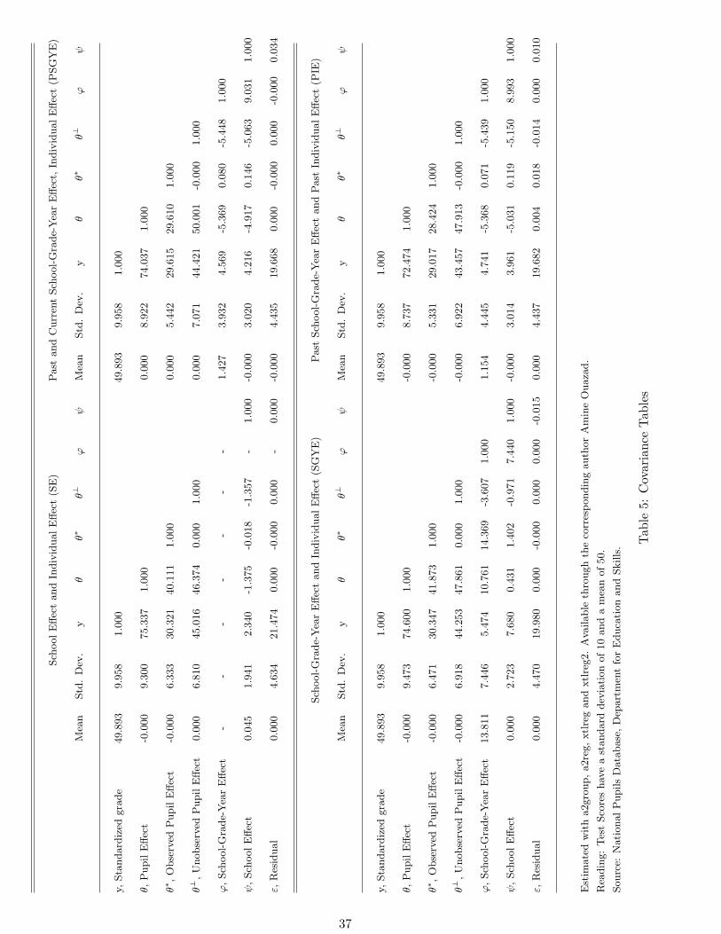
Sch

ool

Eff

ect

and

Indiv

idual

Eff

ect

(SE

)P

ast

and

Curr

ent

Sch

ool-

Gra

de-

Yea

rE

ffec

t,In

div

idual

Eff

ect

(PSG

YE

)

Mea

nStd

.D

ev.

yθ

θ∗

θ⊥

ϕψ

Mea

nStd

.D

ev.

yθ

θ∗

θ⊥

ϕψ

y,Sta

ndard

ized

gra

de

49.8

93

9.9

58

1.0

00

49.8

93

9.9

58

1.0

00

θ,

Pupil

Eff

ect

-0.0

00

9.3

00

75.3

37

1.0

00

0.0

00

8.9

22

74.0

37

1.0

00

θ∗,

Obse

rved

Pupil

Eff

ect

-0.0

00

6.3

33

30.3

21

40.1

11

1.0

00

0.0

00

5.4

42

29.6

15

29.6

10

1.0

00

θ⊥

,U

nobse

rved

Pupil

Eff

ect

0.0

00

6.8

10

45.0

16

46.3

74

0.0

00

1.0

00

0.0

00

7.0

71

44.4

21

50.0

01

-0.0

00

1.0

00

ϕ,

Sch

ool-

Gra

de-

Yea

rE

ffec

t-

--

--

--

1.4

27

3.9

32

4.5

69

-5.3

69

0.0

80

-5.4

48

1.0

00

ψ,

Sch

ool

Eff

ect

0.0

45

1.9

41

2.3

40

-1.3

75

-0.0

18

-1.3

57

-1.0

00

-0.0

00

3.0

20

4.2

16

-4.9

17

0.1

46

-5.0

63

9.0

31

1.0

00

ε,R

esid

ual

0.0

00

4.6

34

21.4

74

0.0

00

-0.0

00

0.0

00

-0.0

00

-0.0

00

4.4

35

19.6

68

0.0

00

-0.0

00

0.0

00

-0.0

00

0.0

34

Sch

ool-

Gra

de-

Yea

rE

ffec

tand

Indiv

idual

Eff

ect

(SG

YE

)P

ast

Sch

ool-

Gra

de-

Yea

rE

ffec

tand

Past

Indiv

idual

Eff

ect

(PIE

)

Mea

nStd

.D

ev.

yθ

θ∗

θ⊥

ϕψ

Mea

nStd

.D

ev.

yθ

θ∗

θ⊥

ϕψ

y,Sta

ndard

ized

gra

de

49.8

93

9.9

58

1.0

00

49.8

93

9.9

58

1.0

00

θ,

Pupil

Eff

ect

-0.0

00

9.4

73

74.6

00

1.0

00

-0.0

00

8.7

37

72.4

74

1.0

00

θ∗,

Obse

rved

Pupil

Eff

ect

-0.0

00

6.4

71

30.3

47

41.8

73

1.0

00

-0.0

00

5.3

31

29.0

17

28.4

24

1.0

00

θ⊥

,U

nobse

rved

Pupil

Eff

ect

-0.0

00

6.9

18

44.2

53

47.8

61

0.0

00

1.0

00

-0.0

00

6.9

22

43.4

57

47.9

13

-0.0

00

1.0

00

ϕ,

Sch

ool-

Gra

de-

Yea

rE

ffec

t13.8

11

7.4

46

5.4

74

10.7

61

14.3

69

-3.6

07

1.0

00

1.1

54

4.4

45

4.7

41

-5.3

68

0.0

71

-5.4

39

1.0

00

ψ,

Sch

ool

Eff

ect

0.0

00

2.7

23

7.6

80

0.4

31

1.4

02

-0.9

71

7.4

40

1.0

00

-0.0

00

3.0

14

3.9

61

-5.0

31

0.1

19

-5.1

50

8.9

93

1.0

00

ε,R

esid

ual

0.0

00

4.4

70

19.9

80

0.0

00

-0.0

00

0.0

00

0.0

00

-0.0

15

0.0

00

4.4

37

19.6

82

0.0

04

0.0

18

-0.0

14

0.0

00

0.0

10

Est

imate

dw

ith

a2gro

up,

a2re

g,

xtl

reg

and

xtl

reg2.

Ava

ilable

thro

ugh

the

corr

esp

ondin

gauth

or

Am

ine

Ouaza

d.

Rea

din

g:

Tes

tSco

res

hav

ea

standard

dev

iati

on

of

10

and

am

ean

of

50.

Sourc

e:N

ati

onal

Pupils

Data

base

,D

epart

men

tfo

rE

duca

tion

and

Skills

.

Tab

le5:

Cov

aria

nce

Tab

les

37

Dependent variable: Pupil Fixed EffectSample: Key Stage 1 and Key Stage 2

Specification

(SE) (SGYE) (PSGYE) (PIE)

Male 0.259** 0.256** 0.254** 0.255**( 0.010 ) ( 0.010 ) ( 0.011 ) ( 0.010 )

Free School Meal -4.097** -4.080** -4.067** -3.987**( 0.015 ) ( 0.015 ) ( 0.015 ) ( 0.015 )

Special Needs -11.268** -11.238** -11.287** -11.064**( 0.014 ) ( 0.014 ) ( 0.014 ) ( 0.014 )

Month Of Birth -0.274** -0.276** -0.276** -0.268**( 0.001 ) ( 0.001 ) ( 0.001 ) ( 0.001 )

Chinese 1.633** 1.567** 1.644** 1.622**( 0.094 ) ( 0.096 ) ( 0.097 ) ( 0.095 )

Mixed 0.449** 0.395** 0.426** 0.415**( 0.039 ) ( 0.040 ) ( 0.041 ) ( 0.039 )

Indian -0.643** -0.777** -0.755** -0.733**( 0.034 ) ( 0.035 ) ( 0.035 ) ( 0.034 )

White Ref. Ref. Ref. Ref.

Bangladeshi -3.124** -3.456** -3.429** -3.350**( 0.058 ) ( 0.059 ) ( 0.059 ) ( 0.058 )

Black African -1.794** -2.004** -1.930** -1.882**( 0.048 ) ( 0.048 ) ( 0.049 ) ( 0.047 )

Pakistani -4.028** -3.993** -3.970** -3.874**( 0.036 ) ( 0.036 ) ( 0.036 ) ( 0.035 )

Black, Other -0.855** -1.018** -0.965** -0.957**( 0.073 ) ( 0.074 ) ( 0.075 ) ( 0.073 )

Other ethnicity -0.525** -0.587** -0.556** -0.529**( 0.027 ) ( 0.027 ) ( 0.028 ) ( 0.027 )

Black Carribean -1.540** -1.631** -1.571** -1.548**( 0.045 ) ( 0.045 ) ( 0.045 ) ( 0.044 )

R Squared 0.46 0.47 0.37 0.37

F Statistic 72,860.81 74,926.46 49,801.00 49,851.24

Number of Pupils 1,783,255 1,783,255 1,783,255 1,783,255

Source: National Pupils Database, Department for Education and Skills.

**: Significant at 1%. *: Significant at 5%.

Reading: Test Scores have a standard deviation of 10 and a mean of 50.

Table 6: Analysis of Pupil Fixed Effects

38

Dependent variable: ϕj,g,t School-Grade-Year Effect

Grade 2 Grade 6

Specification (SGYE) (PSGYE) (PIE) (SGYE) (PSGYE) (PIE)

Fraction in GradeMale -0.445** -0.395* -0.390* 0.777** 0.867** 0.906**

( 0.157 ) ( 0.181 ) ( 0.178 ) ( 0.162 ) ( 0.182 ) ( 0.185 )

Free School Meal 0.678** 0.536* 0.458 -0.465* -0.712** -0.660**( 0.236 ) ( 0.257 ) ( 0.252 ) ( 0.230 ) ( 0.242 ) ( 0.246 )

Special Needs -0.171 -0.329 -0.586** -0.206 -0.290 -0.061( 0.175 ) ( 0.198 ) ( 0.195 ) ( 0.163 ) ( 0.180 ) ( 0.182 )

White Ref. Ref. Ref. Ref. Ref. Ref.

Chinese -2.063 -3.412 -3.233 5.128** 4.436** 4.577**( 1.685 ) ( 1.790 ) ( 1.766 ) ( 1.645 ) ( 1.689 ) ( 1.712 )

Mixed -0.873 -0.954 -1.066 0.222 0.143 0.239( 0.541 ) ( 0.586 ) ( 0.577 ) ( 0.526 ) ( 0.553 ) ( 0.562 )

Indian -0.490 -0.715 -0.619 1.965* 1.866* 1.816*( 0.801 ) ( 0.857 ) ( 0.849 ) ( 0.787 ) ( 0.816 ) ( 0.832 )

Bangladeshi -1.802 -1.624 -1.481 0.223 0.387 0.463( 1.763 ) ( 1.781 ) ( 1.773 ) ( 1.292 ) ( 1.275 ) ( 1.341 )

Black African -1.205 -0.830 -0.733 0.933 0.935 0.850( 0.886 ) ( 0.934 ) ( 0.927 ) ( 0.744 ) ( 0.755 ) ( 0.762 )

Pakistani 0.521 0.350 0.470 1.314 1.242 1.347( 0.818 ) ( 0.860 ) ( 0.844 ) ( 0.711 ) ( 0.717 ) ( 0.726 )

Black, Other 1.903 1.637 1.750 -0.020 -0.173 -0.390( 1.020 ) ( 1.085 ) ( 1.070 ) ( 0.958 ) ( 1.002 ) ( 1.011 )

Black Carribean 0.649 0.467 0.593 -3.030** -3.195** -3.192**( 0.841 ) ( 0.882 ) ( 0.875 ) ( 0.781 ) ( 0.798 ) ( 0.808 )

School Fixed Effects Yes Yes Yes Yes Yes Yes

R Squared 0.87 0.75 0.79 0.92 0.62 0.69

F Statistic 10,814.15 3,956.89 5,686.27 18,246.64 845.84 2,250.07

Number of observations 8,660,468 8,660,468 8,660,468 8,660,468 8,660,468 8,660,468

Number of school-grade-years 96,154 96,154 96,154 96,154 96,154 96,154

Number of schools 20,705 20,705 20,705 20,705 20,705 20,705

Source: National Pupils Database, Department for Education and Skills.

**: Significant at 1%. *: Significant at 5%.

Reading: Test Scores have a standard deviation of 10 and a mean of 50.

Table 7: Peer Effects in Schools – Analysis of School-Grade-Year Effects

39

Dep

enden

tva

riable

:ψj

Sch

ool

Eff

ect

Gra

de

2G

rade

6

Sp

ecifi

cati

on

(SE

)(S

GY

E)

(PSG

YE

)(P

IE)

(SE

)(S

GY

E)

(PSG

YE

)(P

IE)

Sch

oolSta

tus

Com

munit

yR

ef.

Ref

.R

ef.

Ref

.R

ef.

Ref

.R

ef.

Ref

.

Volu

nta

ryA

ided

0.0

02

-0.0

31

0.0

49

0.0

61

0.2

77**

0.4

26**

0.3

98**

0.3

68**

(0.0

47

)(

0.0

54

)(

0.0

61

)(

0.0

60

)(

0.0

52

)(

0.0

56

)(

0.0

68

)(

0.0

69

)

Volu

nta

ryC

ontr

olled

-0.4

30**

-0.3

72**

-0.2

15**

-0.1

94**

-0.2

70**

-0.2

93**

-0.2

30**

-0.2

48**

(0.0

55

)(

0.0

62

)(

0.0

71

)(

0.0

70

)(

0.0

61

)(

0.0

67

)(

0.0

80

)(

0.0

81

)

Foundati

on

0.0

93

0.0

84

0.0

74

0.0

89

0.2

01

0.1

46

0.0

12

-0.0

21

(0.1

49

)(

0.1

69

)(

0.1

93

)(

0.1

91

)(

0.1

49

)(

0.1

62

)(

0.1

95

)(

0.1

97

)

Com

munit

ySp

ecia

l-3

.367**

-4.8

75**

0.8

76**

0.8

76**

-3.4

04**

-4.3

15**

-1.6

43**

-0.8

77**

(0.1

04

)(

0.1

17

)(

0.1

33

)(

0.1

32

)(

0.1

02

)(

0.1

12

)(

0.1

34

)(

0.1

36

)

Non-M

ain

tain

edSp

ecia

l-2

.496*

3.6

59**

4.6

79**

4.8

14**

-5.0

62**

-4.7

73**

-4.6

51**

-3.9

31**

(0.9

93

)(

1.1

31

)(

1.2

92

)(

1.2

78

)(

0.4

60

)(

0.5

02

)(

0.6

05

)(

0.6

12

)

Foundati

on

Sp

ecia

l-4

.442**

-6.5

71**

-2.7

78**

-2.7

37**

-4.6

86**

-5.3

12**

-3.5

47**

-2.8

70**

(0.7

69

)(

0.8

76

)(

1.0

01

)(

0.9

90

)(

0.8

22

)(

0.8

97

)(

1.0

80

)(

1.0

93

)

RSquare

d0.0

70.1

00.0

00.0

00.0

80.1

00.0

20.0

1

FSta

tist

ic159.8

3229.8

710.4

610.0

2182.4

5228.1

436.3

418.1

7

Num

ber

of

obse

rvati

ons

17,4

82

17,4

82

17,4

82

17,4

82

16,1

97

16,1

97

16,1

97

16,1

97

Sourc

e:N

ati

onal

Pupils

Data

base

,D

epart

men

tfo

rE

duca

tion

and

Skills

.

**:

Sig

nifi

cant

at

1%

.*:

Sig

nifi

cant

at

5%

.

Rea

din

g:

Tes

tSco

res

hav

ea

standard

dev

iati

on

of

10

and

am

ean

of

50.

Tab

le8:

The

Ana

lysi

sof

Scho

olE

ffect

s

40

Pas

tan

dC

urre

ntSc

hool

-Gra

de-Y

ear

Effe

cts

(PSG

YE

)19

98-2

002

Coh

ort

1999

-200

3C

ohor

t20

00-2

004

Coh

ort

λσ

χ2

Stat

isti

cp-v

alue

σχ

2St

atis

tic

p-v

alue

σχ

2St

atis

tic

p-v

alue

0.0

Ref

.R

ef.

Ref

.+

0.00

90.

004

0.95

0R

ef.

Ref

.R

ef.

0.1

+0.

022

<0.

000

>0.

999

Ref

.R

ef.

Ref

.+

0.00

1<

0.00

00.

983

0.2

+0.

022

<0.

000

>0.

999

+0.

001

<0.

000

0.98

4+

0.00

9<

0.00

00.

984

0.3

+0.

022

<0.

000

>0.

999

+0.

018

0.00

80.

929

+0.

010

<0.

000

0.98

30.

4+

0.02

2<

0.00

0>

0.99

9+

0.01

40.

006

0.93

8+

0.00

1<

0.00

00.

983

0.5

+0.

022

<0.

000

>0.

999

+0.

014

0.00

60.

938

+0.

001

<0.

000

0.98

30.

6+

0.02

2<

0.00

0>

0.99

9+

0.00

90.

004

0.95

0+

0.00

2<

0.00

00.

983

0.7

+0.

022

<0.

000

>0.

999

+0.

024

0.01

00.

919

+0.

029

0.01

30.

909

0.8

+51

.700

5.01

40.

025

+3.

777

3.26

30.

071

+0.

134

0.06

00.

806

0.9

+11

3.13

76.

547

0.01

0+

61.7

605.

304

0.02

1+

7.94

82.

074

0.15

0

Pas

tan

dC

urre

ntSc

hool

-Gra

de-Y

ear

Effe

cts

(PIE

)19

98-2

002

Coh

ort

1999

-200

3C

ohor

t20

00-2

004

Coh

ort

λσ

χ2

Stat

isti

cp-v

alue

σχ

2St

atis

tic

p-v

alue

σχ

2St

atis

tic

p-v

alue

0.0

Ref

.R

ef.

Ref

.+

261,

013.

403

21.8

60<

0.00

0R

ef.

Ref

.R

ef.

0.1

+75

0118

.678

24.0

76<

0.00

0R

ef.

Ref

.R

ef.

+21

4,66

1.45

721

.601

<0.

000

0.2

+1,

839,

323.

563

25.8

60<

0.00

0+

323,

750.

729

22.2

90<

0.00

0+

917,

322.

339

24.3

72<

0.00

00.

3+

3,14

3,21

9.04

226

.942

<0.

000

+1,

052,

877.

902

24.6

50<

0.00

0+

1,94

8,03

5.81

525

.879

<0.

000

0.4

+4,

572,

608.

331

27.6

91<

0.00

0+

2,05

5,04

2.30

225

.987

<0.

000

+3,

190,

195.

853

26.8

67<

0.00

00.

5+

6,06

4,57

5.91

828

.256

<0.

000

+3,

233,

857.

100

26.8

90<

0.00

0+

4,55

9,96

8.80

427

.580

<0.

000

0.6

+7,

575,

442.

735

28.7

01<

0.00

0+

4,51

9,81

7.45

427

.524

<0.

000

+5,

997,

791.

130

28.1

30<

0.00

00.

7+

9,07

5,42

5.54

129

.063

<0.

000

+5,

863,

248.

922

28.0

82<

0.00

0+

7,46

1,83

9.45

028

.566

<0.

000

0.8

+10

,544

,684

.720

29.3

63<

0.00

0+

7,22

8,98

2.82

233

.107

<0.

000

+8,

923,

139.

887

28.9

23<

0.00

00.

9+

11,9

70,4

44.4

9029

.616

<0.

000

+8,

592,

403.

857

28.8

50<

0.00

0+

10,3

61,9

76.8

7029

.222

<0.

000

Est

imate

dw

ith

a2gro

up,

a2re

g,

xtl

reg

and

xtl

reg2.

Ava

ilable

thro

ugh

the

corr

esp

ondin

gauth

or

Am

ine

Ouaza

d.

See

app

endix

Bfo

rth

ees

tim

ati

on

tech

niq

ue

forλ

.

Sourc

e:N

ati

onal

Pupils

Data

base

,D

epart

men

tfo

rE

duca

tion

and

Skills

.

Under

the

hyp

oth

esis

thatλ

iseq

ual

toit

sopti

mal

valu

eλ∗

(0fo

r1998-2

002

and

2000-2

004,

0.1

for

1999-2

003),

the

stati

stic

2·ln

(L(λ∗)/L

(λ))

conver

ges

toaχ

2st

ati

stic

.T

he

stati

stic

isre

port

edin

colu

mn

3and

the

p-v

alu

eof

the

test

inco

lum

n4.

Tab

le9:

Pas

tan

dC

urre

ntSc

hool

-Gra

de-Y

ear

Effe

cts

-R

esid

ual

Sum

ofSq

uare

san

dth

eD

isco

unti

ngFa

ctorλ

41

Dependent variableMover Moving to School-Grade-Year School

the most frequent school effects effects

Past School-Grade-Year Effect -0.003** 0.001** 0.563** 0.007**( 0.000 ) ( 0.000 ) ( 0.002 ) ( 0.001 )

Past School Effect 0.020** 0.018** -0.214** 0.341**( 0.000 ) ( 0.000 ) ( 0.002 ) ( 0.002 )

Past Pupil Effect -0.003** 0.001** -0.051** -0.023**( 0.000 ) ( 0.000 ) ( 0.000 ) ( 0.000 )

Male 0.000 0.001 0.034** -0.007*( 0.001 ) ( 0.001 ) ( 0.004 ) ( 0.003 )

Free School Meal 0.032** -0.031** -0.148** 0.074**( 0.001 ) ( 0.001 ) ( 0.006 ) ( 0.005 )

Special Needs -0.015** -0.002 -0.613** -0.319**( 0.001 ) ( 0.001 ) ( 0.006 ) ( 0.005 )

Month Of Birth 0.000 0.001** -0.005** -0.004**( 0.000 ) ( 0.000 ) ( 0.001 ) ( 0.000 )

Chinese 0.014 -0.026** 0.492** 0.236**( 0.007 ) ( 0.006 ) ( 0.037 ) ( 0.031 )

Mixed 0.007* -0.027** 0.320** 0.281**( 0.003 ) ( 0.002 ) ( 0.016 ) ( 0.013 )

Indian 0.017** 0.039** 0.529** 0.009( 0.003 ) ( 0.002 ) ( 0.014 ) ( 0.011 )

Bangladeshi -0.114** -0.047** 1.509** 1.213**( 0.004 ) ( 0.003 ) ( 0.027 ) ( 0.022 )

Black African -0.038** -0.087** 0.823** 0.939**( 0.004 ) ( 0.003 ) ( 0.022 ) ( 0.018 )

Pakistani -0.068** -0.010** 0.473** 0.136**( 0.002 ) ( 0.002 ) ( 0.014 ) ( 0.012 )

Black, Other 0.011* -0.037** 0.295** 0.548**( 0.006 ) ( 0.005 ) ( 0.031 ) ( 0.026 )

Black Carribean -0.054** -0.057** 0.390** 0.803**( 0.003 ) ( 0.003 ) ( 0.019 ) ( 0.016 )

Number of observations 3,335,640 3,335,640 3,335,640 3,335,640

R Squared 0.01 0.01 0.52 0.16

F Statistic 1,019.03 1,289.69 71,912.88 8,117.50

Source: National Pupils Database, Department for Education and Skills.

**: Significant at 1%. *: Significant at 5%.

Reading: Test Scores have a standard deviation of 10 and a mean of 50.

Table 10: An Analysis of Mobility and the Direction of Mobility– Between Grade 2 and Grade 6

42

Number of Pupils 1,783,255 pupils (100.00 %). . . with 2 years of observation 1,674,286 pupils ( 93.89 %)

. . . changing school 750,022 pupils ( 42.06 %)

Percentage of moving pupils

Compulsory move 546,800 pupils ( 72.90 %)Non-compulsory move 203,222 pupils ( 27.10 %)

Changing School Type 199,868 pupils ( 26.65 %)Changing LEA 112,592 pupils ( 15.01 %)Moving to the most frequent school 473,231 pupils ( 63.10 %). . . among compulsory movers 423,995 pupils ( 56.53 %). . . among non-compulsory movers 49,236 pupils ( 6.56 %)

Compulsory movers: the pupil had to move, for his Key Stage 1 does not cater for Key Stage 2 pupils. Noncompulsory

movers: the pupil could have staid in the same school for both Key Stage 1 and 2.

Source: National Pupils Database, Department for Education and Skills.

Table 11: Descriptive Statistics on Mobility

43

Cannot stay Can Stay in the Same Schoolin the same school Movers Stayers

Moving to the most frequent school 0.776 0.151 -( 0.417 ) ( 0.358 ) -

Male 0.508 0.509 0.507( 0.500 ) ( 0.500 ) ( 0.500 )

Month Of Birth 6.532 6.546 6.481( 3.557 ) ( 3.574 ) ( 3.589 )

Special Needs 0.213 0.267 0.214( 0.409 ) ( 0.442 ) ( 0.410 )

Free School Meal 0.156 0.244 0.156( 0.363 ) ( 0.429 ) ( 0.362 )

English spoken at home 0.928 0.920 0.915( 0.259 ) ( 0.272 ) ( 0.279 )

White 0.868 0.837 0.856( 0.338 ) ( 0.370 ) ( 0.352 )

Black Carribean 0.010 0.017 0.014( 0.101 ) ( 0.131 ) ( 0.118 )

Black, Other 0.004 0.007 0.004( 0.064 ) ( 0.085 ) ( 0.067 )

Pakistani 0.022 0.021 0.026( 0.146 ) ( 0.144 ) ( 0.160 )

Black African 0.008 0.019 0.012( 0.087 ) ( 0.137 ) ( 0.107 )

Mixed 0.017 0.024 0.018( 0.128 ) ( 0.154 ) ( 0.133 )

Bangladeshi 0.007 0.008 0.010( 0.084 ) ( 0.089 ) ( 0.099 )

Indian 0.023 0.018 0.020( 0.151 ) ( 0.132 ) ( 0.141 )

Chinese 0.003 0.003 0.003( 0.050 ) ( 0.057 ) ( 0.051 )

Compulsory movers: the pupil had to move, for his Key Stage 1 does not cater for Key Stage 2 pupils. Noncompulsory

movers: the pupil could have staid in the same school for both Key Stage 1 and 2.

Source: National Pupils Database, Department for Education and Skills.

Table 12: The characteristics of compulsory movers, noncompulsory movers and nonmovers

44

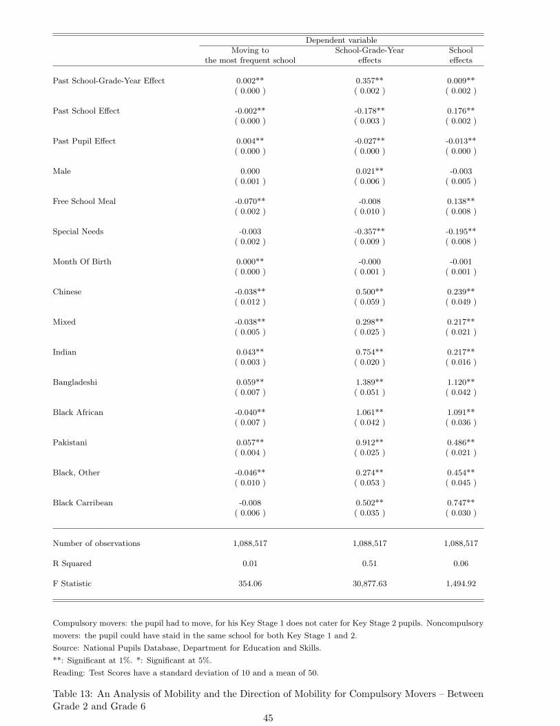
Dependent variableMoving to School-Grade-Year School

the most frequent school effects effects

Past School-Grade-Year Effect 0.002** 0.357** 0.009**( 0.000 ) ( 0.002 ) ( 0.002 )

Past School Effect -0.002** -0.178** 0.176**( 0.000 ) ( 0.003 ) ( 0.002 )

Past Pupil Effect 0.004** -0.027** -0.013**( 0.000 ) ( 0.000 ) ( 0.000 )

Male 0.000 0.021** -0.003( 0.001 ) ( 0.006 ) ( 0.005 )

Free School Meal -0.070** -0.008 0.138**( 0.002 ) ( 0.010 ) ( 0.008 )

Special Needs -0.003 -0.357** -0.195**( 0.002 ) ( 0.009 ) ( 0.008 )

Month Of Birth 0.000** -0.000 -0.001( 0.000 ) ( 0.001 ) ( 0.001 )

Chinese -0.038** 0.500** 0.239**( 0.012 ) ( 0.059 ) ( 0.049 )

Mixed -0.038** 0.298** 0.217**( 0.005 ) ( 0.025 ) ( 0.021 )

Indian 0.043** 0.754** 0.217**( 0.003 ) ( 0.020 ) ( 0.016 )

Bangladeshi 0.059** 1.389** 1.120**( 0.007 ) ( 0.051 ) ( 0.042 )

Black African -0.040** 1.061** 1.091**( 0.007 ) ( 0.042 ) ( 0.036 )

Pakistani 0.057** 0.912** 0.486**( 0.004 ) ( 0.025 ) ( 0.021 )

Black, Other -0.046** 0.274** 0.454**( 0.010 ) ( 0.053 ) ( 0.045 )

Black Carribean -0.008 0.502** 0.747**( 0.006 ) ( 0.035 ) ( 0.030 )

Number of observations 1,088,517 1,088,517 1,088,517

R Squared 0.01 0.51 0.06

F Statistic 354.06 30,877.63 1,494.92

Compulsory movers: the pupil had to move, for his Key Stage 1 does not cater for Key Stage 2 pupils. Noncompulsory

movers: the pupil could have staid in the same school for both Key Stage 1 and 2.

Source: National Pupils Database, Department for Education and Skills.

**: Significant at 1%. *: Significant at 5%.

Reading: Test Scores have a standard deviation of 10 and a mean of 50.

Table 13: An Analysis of Mobility and the Direction of Mobility for Compulsory Movers – BetweenGrade 2 and Grade 6

45

Sch

ool

Eff

ect

and

Indiv

idual

Eff

ect

(SE

)P

ast

and

Curr

ent

Sch

ool-

Gra

de-

Yea

rE

ffec

t,In

div

idual

Eff

ect

(PSG

YE

)

Mea

nStd

.D

ev.

yθ

θ∗

θ⊥

ϕψ

Mea

nStd

.D

ev.

yθ

θ∗

θ⊥

ϕψ

y,Sta

ndard

ized

gra

de

50.0

66

9.7

73

1.0

00

50.0

66

9.7

73

1.0

00

θ,

Pupil

Eff

ect

-0.0

00

9.1

91

0.8

12

1.0

00

-0.0

00

9.3

60

0.7

91

1.0

00

θ∗,

Obse

rved

Pupil

Eff

ect

-0.0

00

6.2

52

0.4

75

0.6

80

1.0

00

-0.0

00

6.3

26

0.4

68

0.6

76

1.0

00

θ⊥

,U

nobse

rved

Pupil

Eff

ect

-0.0

00

6.7

37

0.6

67

0.7

33

-0.0

00

1.0

00

-0.0

00

6.8

98

0.6

44

0.7

37

-0.0

00

1.0

00

ϕ,

Sch

ool-

Gra

de-

Yea

rE

ffec

t-

--

--

--

13.4

24

5.8

75

0.1

13

0.0

14

0.1

32

-0.1

02

1.0

00

ψ,

Sch

ool

Eff

ect

8.2

41

6.9

38

0.0

74

-0.0

34

-0.0

17

-0.0

31

-1.0

00

-0.0

00

2.1

45

0.1

24

-0.0

92

-0.0

04

-0.1

21

0.3

55

1.0

00

ε,R

esid

ual

0.0

00

4.3

64

0.4

47

-0.0

00

-0.0

00

0.0

00

-0.0

00

-0.0

00

4.2

77

0.4

38

-0.0

00

-0.0

00

0.0

00

-0.0

00

0.0

00

Est

imate

dw

ith

a2gro

up,

a2re

g,

xtl

reg

and

xtl

reg2.

Ava

ilable

thro

ugh

the

corr

esp

ondin

gauth

or

Am

ine

Ouaza

d.

Sourc

e:N

ati

onal

Pupils

Data

base

,D

epart

men

tfo

rE

duca

tion

and

Skills

.

Tab

le14

:C

orre

lati

onT

able

s–

Com

puls

ory

mov

ers

only

46

(a) Fraction Male (b) Fraction on Free School Meals

(c) Fraction of Special Needs (d) Fraction Chinese

(e) Fraction Indian (f) Fraction Black African

See section 5.3 for the description of the simulation procedure. Inspired by Lavy and Schlosser (2007).

Figure 2: Year to year variations in grade composition - Realized vs simulated deviations

47

Overall Variance Between Schools Between LEAs Between School Types

Key Stage 1Test Scores 99.006 16.172 1.094 3.475

( 100.0 %) ( 16.3 %) ( 1.1 %) ( 3.5 %)Individual Effects 76.607 17.278 1.755 2.922

( 100.0 %) ( 22.6 %) ( 2.3 %) ( 3.8 %)School-Grade-Year Effects 23.110 23.110 0.390 0.052

( 100.0 %) ( 100.0 %) ( 1.7 %) ( 0.2 %)School Effects 5.560 5.560 0.406 0.039

( 100.0 %) ( 100.0 %) ( 7.3 %) ( 0.7 %)Key Stage 2Test Scores 99.259 19.339 1.080 5.195

( 100.0 %) ( 19.5 %) ( 1.1 %) ( 5.2 %)Individual Effects 76.162 18.336 1.739 4.371

( 100.0 %) ( 24.1 %) ( 2.3 %) ( 5.7 %)School-Grade-Year Effects 13.924 13.924 0.390 0.057

( 100.0 %) ( 100.0 %) ( 2.8 %) ( 0.4 %)School Effects 5.160 5.160 0.406 0.044

( 100.0 %) ( 100.0 %) ( 7.9 %) ( 0.9 %)

Source: National Pupils Database, Department for Education and Skills.

**: Significant at 1%. *: Significant at 5%.

Reading: Test Scores have a standard deviation of 10 and a mean of 50.

Table 15: Decomposition of Variance

48

– First Simulation –

Mean Std. Dev. y θ ϕ

y, Standardized grade 49.893 9.958 1.000

θ, Pupil Effect 0.000 9.271 -0.001 1.000

ϕ, School-Grade-Year Effect 2.187 6.008 0.012 -0.033 1.000

ε, Residual 17.198 26.010 0.113 0.000 -0.000

– Second Simulation –

Mean Std. Dev. y θ ϕ

y, Standardized grade 49.893 9.958 1.000

θ, Pupil Effect 0.000 9.277 0.000 1.000

ϕ, School-Grade-Year Effect 4.002 6.354 -0.011 -0.033 1.000

ε, Residual 17.201 26.010 0.113 -0.000 -0.000

– Third Simulation –

Mean Std. Dev. y θ ϕ

y, Standardized grade 49.893 9.958 1.000

θ, Pupil Effect -0.000 9.271 0.001 1.000

ϕ, School-Grade-Year Effect -2.960 6.664 0.020 -0.032 1.000

ε, Residual 17.216 26.027 0.112 -0.000 0.000

Source: National Pupils Database, Department for Education and Skills.

Estimated with a2group, a2reg, xtlreg and xtlreg2. Available through the corresponding author Amine Ouazad.

Reading: Test Scores have a standard deviation of 10 and a mean of 50.

Table 16: Correlation Tables – Simulations

49