CDS 101/110: Lecture 2.3Stability (Continue), MATLAB

7 October 2016

Goals:• Review stability of linear systems• A little more detail on Lyapunov Functions• Start of Tutorial on MATLAB functions for control system analysis

Reading: • Åström and Murray, Feedback Systems 2e, Sections 5.1-5.4

The equilibria of system �̇�𝑥 = 𝑓𝑓(𝑥𝑥) are the points xe such that f(xe) = 0.

They represent stationary conditions for the dynamics- Nonlinear systems may have multiple equilibria- Linear systems have only one equilibria (unless characteristic

equation has zero eigenvalues)

2

Equilibrium Points

⇒

An Equilibrium Point is:Stable if initial conditions that start near the equilibrium point, stay near the equilibrium point• Also called “stable in the sense of Lyapunov”• Technical:

- For all 𝜀𝜀 > 0, there exists 𝛿𝛿 > 0 𝑠𝑠. 𝑡𝑡.

𝑥𝑥 0 − 𝑥𝑥𝑒𝑒 < 𝛿𝛿 → 𝑥𝑥 𝑡𝑡 − 𝑥𝑥𝑒𝑒 < 𝜀𝜀 ∀𝑡𝑡 ≥ 0

Asymptotically stable if all initial conditions near equilibrium converge to the equilibrium• Stable + converging• Technical:

- 𝑥𝑥𝑒𝑒 is locally attractive if ∃𝛿𝛿 > 0 s.t. x(0 − xe | < 𝛿𝛿 and lim𝑡𝑡→∞

𝑥𝑥(𝑡𝑡) = 𝑥𝑥𝑒𝑒- 𝑥𝑥𝑒𝑒 is locally asymptotically stable if it is locally stable & locally

attractive

Exponentially stable if it is asymptotically stable and ∃ 𝛼𝛼,𝛽𝛽 > 0 s.t.x(𝑡𝑡 − xe | ≤ α x 0 − xe e−βt t ≥ 0

3

Linear Systems

4

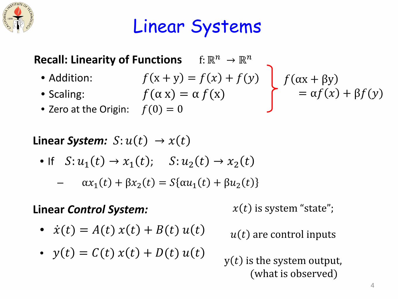
Recall: Linearity of Functions f:ℝ𝑛𝑛 → ℝ𝑛𝑛

• Addition: 𝑓𝑓 x + y = 𝑓𝑓 𝑥𝑥 + 𝑓𝑓(𝑦𝑦)• Scaling: 𝑓𝑓(α x) = α 𝑓𝑓(x)• Zero at the Origin: 𝑓𝑓(0) = 0

𝑓𝑓 αx + βy= α𝑓𝑓 𝑥𝑥 + β𝑓𝑓(𝑦𝑦)

Linear System: 𝑆𝑆:𝑢𝑢 𝑡𝑡 → 𝑥𝑥 𝑡𝑡• If 𝑆𝑆:𝑢𝑢1 𝑡𝑡 → 𝑥𝑥1 𝑡𝑡 ; 𝑆𝑆:𝑢𝑢2 𝑡𝑡 → 𝑥𝑥2 𝑡𝑡

– α𝑥𝑥1 𝑡𝑡 + β𝑥𝑥2 𝑡𝑡 = 𝑆𝑆 α𝑢𝑢1 𝑡𝑡 + β𝑢𝑢2 𝑡𝑡

Linear Control System:

• �̇�𝑥(𝑡𝑡) = 𝐴𝐴(𝑡𝑡) 𝑥𝑥 𝑡𝑡 + 𝐵𝐵(𝑡𝑡) 𝑢𝑢 𝑡𝑡

• 𝑦𝑦 𝑡𝑡 = 𝐶𝐶(𝑡𝑡) 𝑥𝑥 𝑡𝑡 + 𝐷𝐷(𝑡𝑡) 𝑢𝑢 𝑡𝑡

𝑥𝑥 𝑡𝑡 is system “state”;

𝑢𝑢 𝑡𝑡 are control inputs

y 𝑡𝑡 is the system output, (what is observed)

Linear Time Invariant Systems

Linear Time Invariant (LTI) System:

• Given that input 𝑢𝑢(𝑡𝑡) leads to output 𝑦𝑦 𝑡𝑡 , if input 𝑢𝑢(𝑡𝑡 + 𝑇𝑇) leads to output 𝑦𝑦(𝑡𝑡

5

0

0

�̇�𝑥(𝑡𝑡) = 𝐴𝐴𝑥𝑥 𝑡𝑡 + 𝐵𝐵𝑢𝑢(𝑡𝑡)𝑦𝑦 𝑡𝑡 = 𝐶𝐶𝑥𝑥 𝑡𝑡 + 𝐷𝐷𝑢𝑢(𝑡𝑡)

Diagonalized case: Eigenvectors are unique: A is diagonalizable (real, distinct eigenvalues)

Block diagonal case (distinct complex eigenvalues)

Stability of Linear Systems

6

⇒• Stable if λ𝑖𝑖 ≤ 0• Asy stable if λ𝑖𝑖 < 0• Unstable if λ𝑖𝑖 > 0

Coordinate (similarity) Transform: 𝑧𝑧 = 𝑇𝑇𝑥𝑥, where 𝑇𝑇 is invertible• �̇�𝑧 = 𝑇𝑇�̇�𝑥 = 𝑇𝑇𝐴𝐴𝑥𝑥 = 𝑇𝑇𝐴𝐴𝑇𝑇−1𝑧𝑧• If system has equilibrium x = 0, then z = 0 is also an equilibrium• If system is stable in x-coordinates, it is stable in 𝑧𝑧-coordinates• If 𝑇𝑇 is invertible, 𝑒𝑒𝑇𝑇𝑇𝑇𝑇𝑇−1 = 𝑇𝑇𝑒𝑒𝑇𝑇T−1

• System is asy stable if 𝑅𝑅𝑒𝑒 𝜆𝜆𝑖𝑖 = 𝜎𝜎𝑖𝑖 < 0

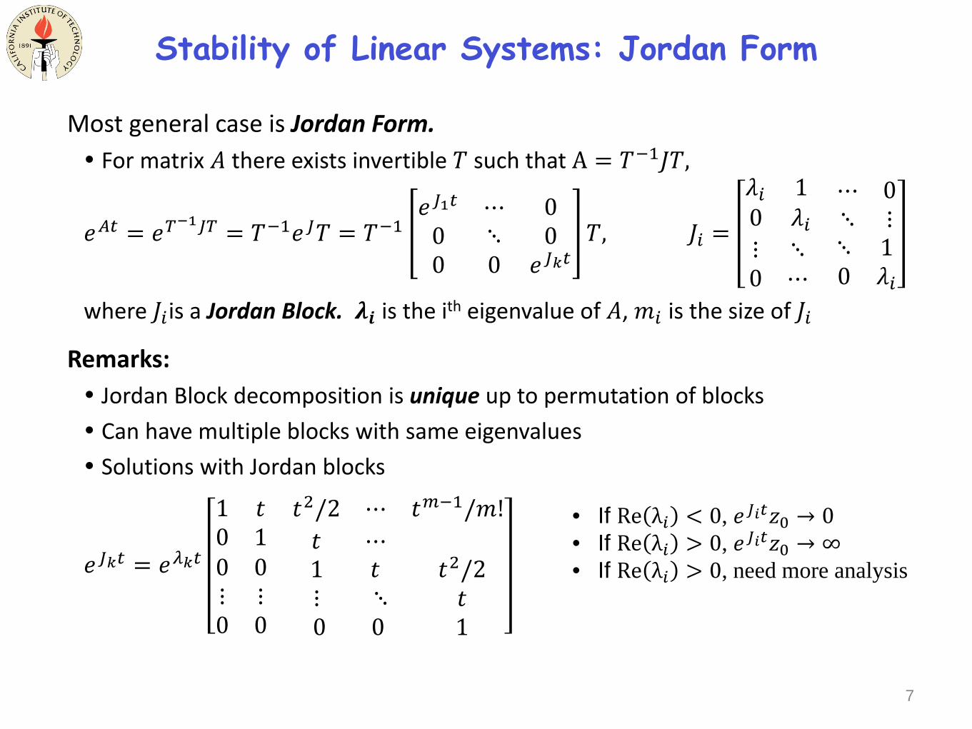
Most general case is Jordan Form. For matrix 𝐴𝐴 there exists invertible 𝑇𝑇 such that A = 𝑇𝑇−1𝐽𝐽𝑇𝑇,

𝑒𝑒𝑇𝑇𝑡𝑡 = 𝑒𝑒𝑇𝑇−1𝐽𝐽𝑇𝑇 = 𝑇𝑇−1𝑒𝑒𝐽𝐽𝑇𝑇 = 𝑇𝑇−1𝑒𝑒𝐽𝐽1𝑡𝑡 ⋯ 0

0 ⋱ 00 0 𝑒𝑒𝐽𝐽𝑘𝑘𝑡𝑡

𝑇𝑇, 𝐽𝐽𝑖𝑖 =

𝜆𝜆𝑖𝑖 10 𝜆𝜆𝑖𝑖

⋯ 0⋱ ⋮

⋮ ⋱0 ⋯

⋱ 10 𝜆𝜆𝑖𝑖

where 𝐽𝐽𝑖𝑖is a Jordan Block. 𝝀𝝀𝒊𝒊 is the ith eigenvalue of 𝐴𝐴, 𝑚𝑚𝑖𝑖 is the size of 𝐽𝐽𝑖𝑖

Remarks: Jordan Block decomposition is unique up to permutation of blocks Can have multiple blocks with same eigenvalues Solutions with Jordan blocks

𝑒𝑒𝐽𝐽𝑘𝑘𝑡𝑡 = 𝑒𝑒𝜆𝜆𝑘𝑘𝑡𝑡

1 𝑡𝑡0 1

𝑡𝑡2/2 ⋯ 𝑡𝑡𝑚𝑚−1/𝑚𝑚!𝑡𝑡 ⋯

0 0⋮ ⋮0 0

1 𝑡𝑡 𝑡𝑡2/2⋮ ⋱ 𝑡𝑡0 0 1

7

Stability of Linear Systems: Jordan Form

• If Re λ𝑖𝑖 < 0, 𝑒𝑒𝐽𝐽𝑖𝑖𝑡𝑡𝑧𝑧0 → 0• If Re λ𝑖𝑖 > 0, 𝑒𝑒𝐽𝐽𝑖𝑖𝑡𝑡𝑧𝑧0 → ∞• If Re λ𝑖𝑖 > 0, need more analysis

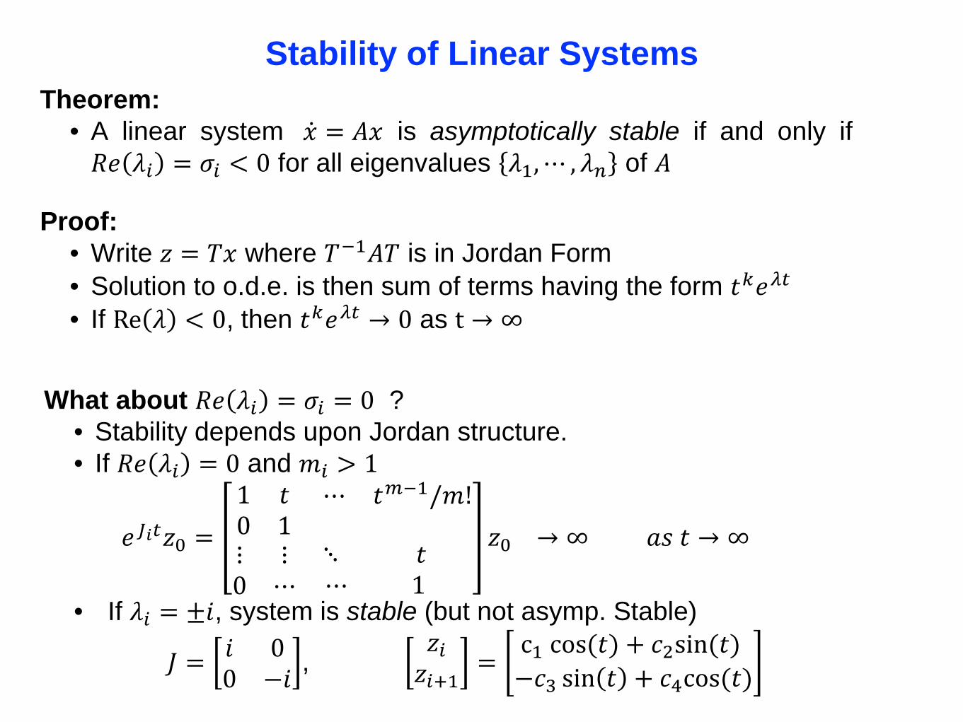
Stability of Linear SystemsTheorem:

• A linear system �̇�𝑥 = 𝐴𝐴𝑥𝑥 is asymptotically stable if and only if𝑅𝑅𝑒𝑒 𝜆𝜆𝑖𝑖 = 𝜎𝜎𝑖𝑖 < 0 for all eigenvalues 𝜆𝜆1,⋯ , 𝜆𝜆𝑛𝑛 of 𝐴𝐴

Proof:• Write 𝑧𝑧 = 𝑇𝑇𝑥𝑥 where 𝑇𝑇−1𝐴𝐴𝑇𝑇 is in Jordan Form• Solution to o.d.e. is then sum of terms having the form 𝑡𝑡𝑘𝑘𝑒𝑒𝜆𝜆𝑡𝑡• If Re 𝜆𝜆 < 0, then 𝑡𝑡𝑘𝑘𝑒𝑒𝜆𝜆𝑡𝑡 → 0 as t → ∞

What about 𝑅𝑅𝑒𝑒 𝜆𝜆𝑖𝑖 = 𝜎𝜎𝑖𝑖 = 0 ?• Stability depends upon Jordan structure.• If 𝑅𝑅𝑒𝑒 𝜆𝜆𝑖𝑖 = 0 and 𝑚𝑚𝑖𝑖 > 1

𝑒𝑒𝐽𝐽𝑖𝑖𝑡𝑡𝑧𝑧0 =1 𝑡𝑡0 1

⋯ 𝑡𝑡𝑚𝑚−1/𝑚𝑚!

⋮ ⋮0 ⋯

⋱ 𝑡𝑡⋯ 1

𝑧𝑧0 → ∞ 𝑎𝑎𝑠𝑠 𝑡𝑡 → ∞

• If 𝜆𝜆𝑖𝑖 = ±𝑖𝑖, system is stable (but not asymp. Stable)

𝐽𝐽 = 𝑖𝑖 00 −𝑖𝑖 ,

𝑧𝑧𝑖𝑖𝑧𝑧𝑖𝑖+1 =

c1 cos(𝑡𝑡) + 𝑐𝑐2sin(𝑡𝑡)−𝑐𝑐3 sin 𝑡𝑡 + 𝑐𝑐4cos(𝑡𝑡)

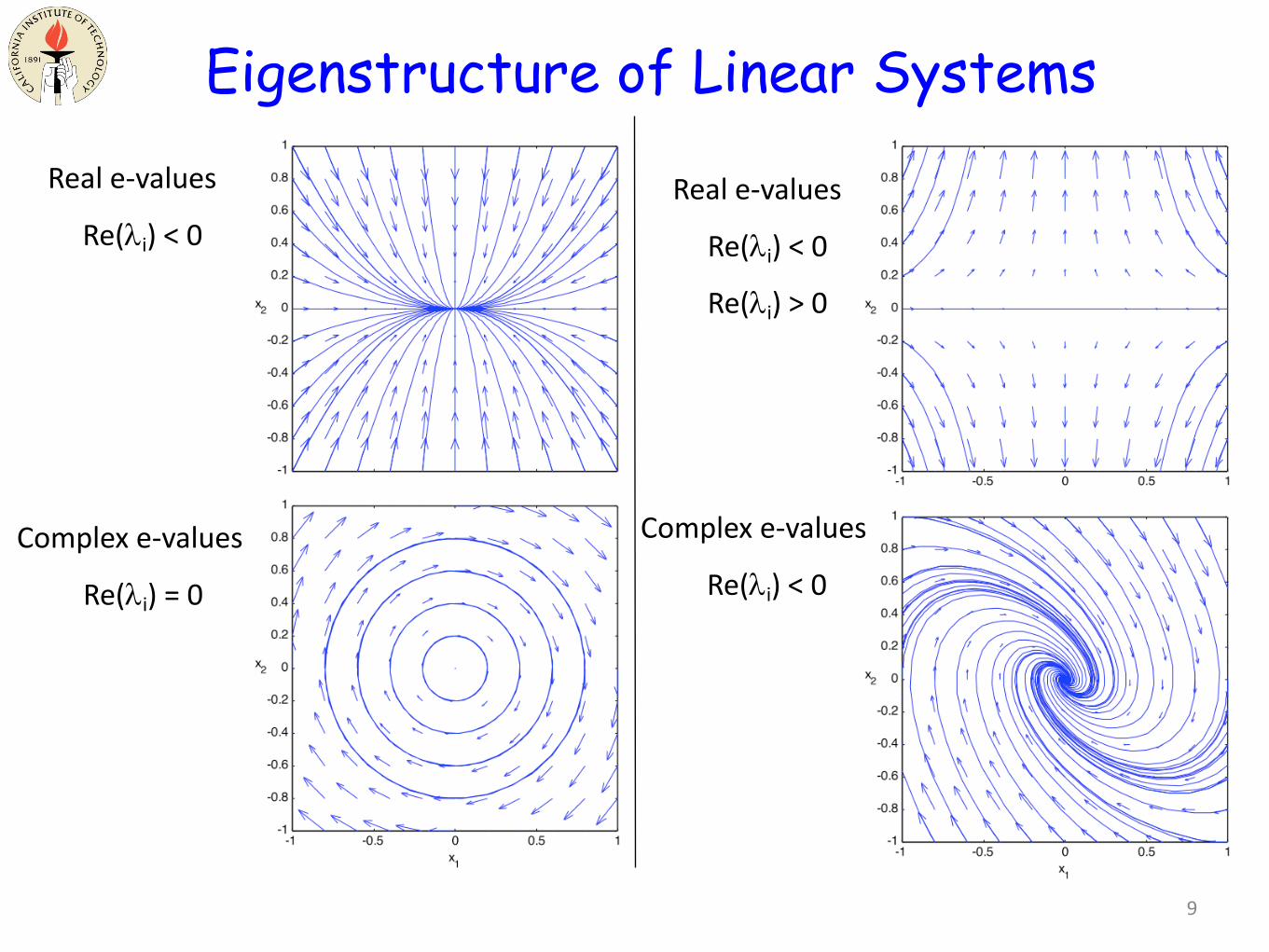
Eigenstructure of Linear Systems

9

Real e-values

Re(λi) < 0Real e-values

Re(λi) < 0

Re(λi) > 0

Complex e-values

Re(λi) = 0

Complex e-values

Re(λi) < 0

10

Linearization Around an Equilibrium Point

Remarks In examples, this is often

equivalent to small angle approximations, etc Only works near to equili-

brium point

-2� 0 2�-2

0

2

x1

x2

Full nonlinear model Linear model (honest!)

“Linearize” around x=xe

11

Local versus Global BehaviorStability is a local concept• Equilibrium points define the local behavior of the dynamical system• Single dynamical system can have stable and unstable equilibrium points

Region of attraction• Set of initial conditions that converge to a given equilibrium point

Basic idea: capture system behavior by tracking its “energy”• Find a single function that captures distance of system from equilibrium• Try to reason about the long term behavior of all solutions, without explicit solution!

Technical: A function 𝑉𝑉:ℝ𝑛𝑛 → ℝ is a Lyapunov function for �̇�𝑥 = 𝑓𝑓(𝑥𝑥)- 𝑉𝑉 0 = 0, 𝑉𝑉 𝑥𝑥 > 0 ∀𝑥𝑥 𝜖𝜖 𝐵𝐵𝑟𝑟\ 0 for 𝐵𝐵𝑟𝑟 a neighborhood of 0 - Note that coordinates can be chosen so that xe = 0

- �̇�𝑉 𝑥𝑥 = 𝑑𝑑𝑑𝑑𝑡𝑡𝑉𝑉 𝑥𝑥 𝑡𝑡 = 𝜕𝜕𝜕𝜕

𝜕𝜕𝜕𝜕� 𝑑𝑑𝜕𝜕𝑑𝑑𝑡𝑡

= 𝜕𝜕𝜕𝜕𝜕𝜕𝜕𝜕� 𝑓𝑓(𝑥𝑥)

- The equilibrium is locally stable if �̇�𝑉 𝑥𝑥 ≤ 0 ∀𝑥𝑥 𝜖𝜖 𝐵𝐵𝑟𝑟\ 0- The equilibrium is locally asymptotically stable if �̇�𝑉 𝑥𝑥 < 0 ∀𝑥𝑥 𝜖𝜖 𝐵𝐵𝑟𝑟\ 0- Artstein’s Thm: if system is stable, a Lyapunov function exists.

Linear Systems: �̇�𝑥 = 𝐴𝐴𝑥𝑥- Consider 𝑉𝑉 𝑥𝑥 = 𝑥𝑥𝑇𝑇𝑃𝑃𝑥𝑥, where 𝑃𝑃𝑇𝑇 = 𝑃𝑃 > 0 (positive definite)

- �̇�𝑉 𝑥𝑥 = 𝜕𝜕𝜕𝜕𝜕𝜕𝜕𝜕� 𝑑𝑑𝜕𝜕𝑑𝑑𝑡𝑡

= 𝑥𝑥𝑇𝑇 𝐴𝐴𝑇𝑇𝑃𝑃 + 𝑃𝑃𝐴𝐴 𝑥𝑥 = −𝑥𝑥𝑇𝑇𝑄𝑄𝑥𝑥

- Lyapunov Equation: 𝐴𝐴𝑇𝑇𝑃𝑃 + 𝑃𝑃𝐴𝐴 = −𝑄𝑄- Can show that solution 𝑃𝑃 exists if 𝐴𝐴 has eigenvalues in left-half plane.

12

Reasoning about Stability using Lyapunov Functions

Lasalle’s Invariance Principle (Barbashin-Krasvoskii-Lasalle)- Gives a way to show asymp. Stability when �̇�𝑉 𝑥𝑥 ≤ 0- Only for time-invariant or periodic systems

Technical:- 𝜔𝜔-limit set of a trajectory 𝑥𝑥 𝑡𝑡, 𝑥𝑥0 is the set of points 𝑝𝑝 such that 𝑥𝑥 𝑡𝑡, 𝑥𝑥0 → 𝑝𝑝 as

t→ ∞ for �̇�𝑥 = 𝑓𝑓(𝑥𝑥).- A set M is said to be invariant if for all 𝑥𝑥0 ∈ 𝑀𝑀, 𝑥𝑥(𝑡𝑡, 𝑥𝑥0) ∈ 𝑀𝑀 for all 𝑡𝑡 ≥ 0- Theorem (5.4, page 5-25): Let 𝑉𝑉:ℝ𝑛𝑛 → ℝ be a locally positive definite function

such that on the compact set Ω𝑟𝑟 = 𝑥𝑥 𝜖𝜖ℝ𝑛𝑛 | 𝑉𝑉(𝑥𝑥) ≤ 𝑟𝑟 , Define𝑆𝑆 = 𝑥𝑥 𝜖𝜖ℝ𝑛𝑛 | �̇�𝑉 𝑥𝑥 = 0 .

as t→ ∞, the trajectory tends to the largest invariant set in S. If S contains noinvariant set except other than x=0, then x=0 is asymptotically stable.

13

Reasoning about Stability using Lyapunov Functions

�̇�𝑉 = −𝑐𝑐𝑥𝑥22.

Continuous time (ODE) version of predator prey dynamics:

Equilibrium points (2)• ~(20.5, 29.5): unstable • (0, 0): unstable

Limit cycle• Population of each species

oscillates over time• Limit cycle is stable (nearby

solutions converge to limit cycle)• This is a global feature of the

dynamics (not local to an equilibrium point)

14

Example #2: Predator Prey (ODE version)

Continuous time (ODE) model MATLAB: predprey.m (from web page)

unstable

stable

Dynamics: • Note that limit cycle is an invariant set• From simulation, x(t+T) = x(t)

Stability of invariant set

Simpler Example of a Limit Cycle

15

16

Summary: Stability and PerformanceKey topics for this lecture• Stability of equilibrium points

• Eigenvalues determine stability for linear systems

• Local versus global behavior