cdot strategic plan for data collection and evaluation … · cdot strategic plan for data...
TRANSCRIPT

Report No. CDOT-2011-11 Final Report
CDOT STRATEGIC PLAN FOR DATA COLLECTION AND EVALUATION OF GRADE 50 H-PILES INTO BEDROCK Nien-Yin Chang Robert Vinopal Cuong Vu Hien Nghiem
August 2011 COLORADO DEPARTMENT OF TRANSPORTATION DTD APPLIED RESEARCH AND INNOVATION BRANCH

The contents of this report reflect the views of the
authors, who are responsible for the facts and accuracy
of the data presented herein. The contents do not
necessarily reflect the official views of the Colorado
Department of Transportation or the Federal Highway
Administration. This report does not constitute a
standard, specification, or regulation. The preliminary
design recommendations should be considered for only
conditions very close to those encountered at the load
test sites and per the qualifications described in Chapter
6. Use of the information contained in the report is at
the sole discretion of the designer.

Technical Report Documentation Page
1. Report No.
CDOT-2011-11 2. Government Accession No.
3. Recipient's Catalog No.
4. Title and Subtitle CDOT STRATEGIC PLAN FOR DATA COLLECTION AND EVALUATION OF GRADE 50 H-PILES INTO BEDROCK
5. Report Date
August 2011
6. Performing Organization Code
UCD-CGES-2010-01 7. Author(s)
Nien-Yin Chang, Ph.D., P.E., Robert Vinopal, Ph.D., Hien Nghiem, Ph.D., and Cuong Vu, PE., Doctoral Candidate
8. Performing Organization Report No.
CDOT-2011-11
9. Performing Organization Name and Address University of Colorado Denver Campus Box 113 P. O. Box 173364 Denver, Colorado 80217
10. Work Unit No. (TRAIS) 11. Contract or Grant No.
12. Sponsoring Agency Name and Address
Colorado Department of Transportation - Research 4201 E. Arkansas Ave. Denver, CO 80222
13. Type of Report and Period Covered
14. Sponsoring Agency Code
80.50
15. Supplementary Notes
Prepared in cooperation with the US Department of Transportation, Federal Highway Administration
16. Abstract This report presents Phase I of CDOT’s effort to address the issues associated with Colorado-specific resistance factors for driven pile designs. As proven during the process of this research, resistance factors vary with geomaterial types and geological locations. Procedures for the driven piles performance data collection for the evaluation of resistance factors for Grade 50 Steel H-piles penetrating into bedrocks are recommended.
The data collection of driven pile performance is planned to continue in Phase II and the benefits of Grade 50 steel piles beyond those of Grade 36 steel piles will be investigated. The research will be expanded to investigate the benefit of using steel driven H-piles with sizes larger than the sizes currently adopted by CDOT, including 18-inch and 24-inch steel H-piles. The benefits in terms of capacity enhancement, pile number reduction in pile group for bridge support, and the associated time and cost savings will be assessed. Different methods for nominal capacity assessment will be used to evaluate the nominal capacities of 18-inch and 24-inch piles. Pile performances will be monitored using pile driving analyzer (PDA), and, if budget permits, load tests will be performed to check the pile capacity calculation. Implementation Successful implementation of geotechnical load and resistance factor design (LRFD) procedures in bridge foundation designs requires Colorado-specific resistance factors. When completed at the end of Phase II, this research is expected to provide Colorado-specific geotechnical resistance factors for steel driven pile designs. 17. Keywords load and resistance factor design (LRFD), driven piles, Grade 36 steel piles, Grade 50 steel piles, GRLWEAP, CAPWAP, standard penetration tests (SPT), O-cell tests, pile driving analyzers (PDA)
18. Distribution Statement
No restrictions. This document is available to the public through the National Technical Information Service www.ntis.gov or CDOT’s Research Report website http://www.coloradodot.info/programs/research/pdfs
19. Security Classif. (of this report)
Unclassified 20. Security Classif. (of this page)
Unclassified 21. No. of Pages
146 22. Price
Form DOT F 1700.7 (8-72) Reproduction of completed page authorized

ii
CDOT STRATEGIC PLAN FOR DATA COLLECTION AND
EVALUATION OF GRADE 50 H-PILES INTO BEDROCK
by
Nien-Yin Chang, Ph.D., P.E., Professor of Civil Engineering Robert Vinopal, Ph.D., Postdoctoral Research Associate
Cuong Vu, Doctoral Candidate and Graduate Research Assistant University of Colorado, Denver
and Hien Nghiem, Ph. D., Lecturer, Hanoi Architectural University, Vietnam
Report No. CDOT-2011-1
Sponsored by the Colorado Department of Transportation
In Cooperation with the U.S. Department of Transportation Federal Highway Administration
August 2011
Colorado Department of Transportation DTD Applied Research and Innovation Branch
4201 E Arkansas Ave Denver, CO 80222

iii
ACKNOWLEDGEMENTS
The opportunity to lead the study on the very important issue of implementation of geotechnical load and resistance factor design is highly appreciated; it presented a great challenge to the Principal Investigator and his research colleagues at the University of Colorado, Denver. A great deal was learned about the strategic plan for the implementation of geotechnical LRFD at CDOT. Discussions with the following study panelists from CDOT were critical in shaping the direction of this research and their efforts are greatly appreciated: Nural Alam, Staff Bridge Alan Hotchkiss, Soils-Rockfall Program Hsing-Cheng Liu, Geotechnical Program Richard Osmun, Staff Bridge C.K. Su, Soils-Rockfall Program Trever Wang, Staff Bridge Aziz Khan, DTD Applied Research and Innovation Branch The contributions and collaboration from Dr. Frank Raushe were particularly invaluable to the implementation of GRLWEAP and CAPWAP in this study and the future adoption of the software for driven pile capacity estimates at CDOT before and after pile installation.

iv
EXECUTIVE SUMMARY
Evidence is clear that the values of geotechnical resistance factors depend on geomaterial and pile material types, design methodologies, and field and/or laboratory evaluation methods for soil parameters. Resistance factors of geomaterials are found to be location dependent, because of the geographical dependency of geomaterial distributions and associated properties. Implementation of geotechnical LRFD foundation design procedures in Colorado requires Colorado-specific resistance factors and procedures for their evaluation. This Phase I study investigated the effect of the shift from Grade 36 to Grade 50 steel on the design and methods for using driven steel piles with tips in rocks. The Phase II study is planned to focus on providing Colorado-specific resistance factors and identify the design methods appropriate for the Colorado Department of Transportation (CDOT).
In this Phase I study, all available CDOT data of driven piles with PDA (pile driving analyzer) monitor and subsurface profiles were collected and analyzed. The following analyses were performed:
� DRIVEN analyses were performed to evaluate the bearing capacity of all piles with both side shear and end bearing components. Three piles were also analyzed using VSPILE program developed independently at UC Denver. The results compared well with those from DRIVEN. DRIVEN output can be used as the input data for pre-installation wave equation analysis, briefed as WEAP analysis.
� WEAP analysis results, including dynamic pile driving stresses, driving resistance (blows per foot of penetration), and energy transfer were used in judging pile drivability and the selection of pile type, hammer, and hammer stroke. For a selected pile type, the pile side shear and end bearing capacities were also evaluated.
� During driving, CDOT monitored the pile performance by pile driving analyzer (PDA). PDA provides strain and acceleration measurements for use in evaluating ultimate pile cap load, velocity, and settlement via signal matching techniques using CAPWAP and the load-settlement curve is generated.
The available data show that CAPWAP capacities provide good estimates for the static ultimate capacities of driven piles. It is recommended that PDA be used in a selected number of piles in each driven pile project and, whenever PDA is used, CAPWAP be performed to assess the ultimate static capacity of driven piles in all Colorado geological conditions.

v
The research shows that Grade 50 steel piles can provide significantly higher capacities than Grade 36 piles, because they can be driven deeper without exceeding their yield stress. The high yield strength also allows the use of a heavier hammer to facilitate pile driving. This means potential cost savings for a bridge project with less required piles.
Implementation Statement Successful implementation of the geotechnical LRFD procedures in bridge foundation designs requires Colorado-specific resistance factors because of their dependency on geomaterial types, design methods, and methods of geomaterials testing. This report presents the results of investigation on the effect of the shift from Grade 36 to Grade 50 steel on the capacity of driven piles and associated potential cost savings. All CDOT driven pile data were collected for those with PDA monitoring. Analyses included static capacity analysis using DRIVEN and VSPILE for comparison, GRLWEAP analyses performed by feeding DRIVEN output or by other parameter input, and signal matching analyses using the CAPWAP program. Various subsurface conditions prevailing in Colorado were involved and all cases were analyzed and results summarized in this report. The procedures were found to be effective for the evaluation of the static pile capacity and beneficial to CDOT driven pile designs, and were recommended for implementation. In driven pile design, it is recommended to:
1. Perform DRIVEN (or VSPile) analysis for the evaluation of the static capacity. The analysis gives both side shear and end bearing resistances.
2. Perform GRLWEAP wave equation analysis, before pile installation, for the evaluation of:
� side shear and end bearing components of pile capacity, � pile driving-induced stresses for judging the feasibility of different hammer
types and hammer strokes to avoid pile damage during driving, and � pile driving resistance in terms of blows per foot of penetration for judging
the feasibility of adopting a hammer type and stroke. 3. Always install PDA during pile driving to monitor pile performance. 4. Provide PDA data for pile capacity calculation using CASE method. 5. Use PDA data in CAPWAP signal matching analysis to further calibrate the
ultimate pile capacity. 6. Collect pile data and statistics to formulate the procedures and equations for the
evaluation of ultimate capacities of piles with tips located in different rock types. 7. Use data from Item 6 in the evaluation of the Colorado-specific geotechnical
resistance factors for driven pile foundation design in Colorado.

vi
TABLE OF CONTENTS
1.0 INTRODUCTION ......................................................................................................1 2.0 COLORADO GEOLOGY, ROCK FORMATION AND STRENGTH .......................3 2.1 Geologic-Geographic Setting ..................................................................................3 2.2 Rock Terminology ..................................................................................................3 2.3 General Geology .....................................................................................................4 2.31 Colorado Piedmont ...........................................................................................5 2.32. Denver Basin ....................................................................................................8 2.3.3 Raton Basin ......................................................................................................10 2.3.4 Intermountain Valleys ......................................................................................11 2.3.5 High Plains in Eastern Colorado ......................................................................12 2.4 Rock Strength of Bearing Stratum ..........................................................................13 2.4.1 Range of Rock Strength along the Front Range ..............................................13 3.0 NOMINAL AXIAL PILE CAPACITY ........................................................................19 3.1 Nominal Axial Capacity of a Driven Pile Using DRIVEN 1.1 ..............................19 3.1.1 Side Resistance in Cohesive Soil .....................................................................19 3.1.2 Tip Resistance in Cohesive Soil ......................................................................21 3.1.3 Side Resistance in Cohesionless Soil – Nordlund Method ............................21 3.1.4 Tip Resistance in Cohesionless Soil – Thurman Method ..............................25 3.2 Soil Properties Evaluated from In-situ Tests ..........................................................27 3.2.1 Undrained Shear Strength Su for Clay Soil .....................................................27 3.2.2 Unconfined Compressive Strength of Claystone Bedrock ..............................27 3.2.3 The Friction Angle for Cohesionless Soil ........................................................27 3.3 Capacity of the H-piles from DRIVEN Program ....................................................28 3.3.1 Capacity of the H-piles in Clay Shale, Shale from DRIVEN Program ...........28 3.3.2 Capacity of the H-piles in Sandstone from DRIVEN Program .......................37 3.3.3 DRIVEN Capacity Estimates for H-piles and Pipe Piles.................................44 3.4 Summary Capacity of the H-piles from Driven 1.1 ................................................47 4.0 WAVE EQUATION ANALYSIS ................................................................................49 4.1 Introduction .............................................................................................................49 4.2 Selection of Input Parameters for GRLWEAP Analyses .......................................49 4.3 Results of GRLWEAP Analyses ............................................................................52 4.3.1 GRLWEAP Analyses of Transmitted Energy .................................................52 4.3.2 GRLWEAP Analysis of Compressive Stress ..................................................54 4.3.3 GRLWEAP Analyses of Driving Resistance ...................................................57 4.4 Summary……………………………………………………………………..…....68

vii
5.0 CAPWAP ANALYSES ................................................................................................70 5.1 Introduction .............................................................................................................70 5.2 CAPWAP Procedures….. .......................................................................................70 5.2.1 Record Selection ..............................................................................................70 5.2.2 Data Adjustment ..............................................................................................71 5.2.3 Pile Model ........................................................................................................71 5.2.4 Signal Matching ...............................................................................................71 5.3 Casetoc 2 Method ...................................................................................................72 5.4 Analysis Results ......................................................................................................726.0 H-PILE LENGTH IN FRONT RANGE ROCKS ........................................................99 6.1 Design Charts for Estimation of H-pile Length ......................................................99 6.2 Pile Length and Pile Capacity in Front Range Rocks .............................................99 6.3 DRIVEN Capacity from Six Different Sites ...........................................................102 6.4 Pile Resistance and Penetration Length ..................................................................107 7.0 SUMMARY, CONCLUSIONS, AND FUTURE STUDY ..........................................110 7.1 Summary .................................................................................................................110 7.2 Findings of this Study .............................................................................................110 7.3 Recommendations for Further Research .................................................................111 REFERENCES ...................................................................................................................113APPENDIX A – BORING LOG PROFILES .....................................................................A-1

1
1.0 INTRODUCTION
Geotechnical resistance factors vary with design methodologies, geomaterial types and methods of testing. In the past, the Colorado Department of Transportation (CDOT) largely used the blow-count based design method for determining geotechnical capacity of driven piles. Alternative methods are available and needed to be explored for application in the Rocky Mountain region. The grade of steel has changed from Grade 36 to Grade 50 for both steel H-piles and pipe piles, so the impact of this change on pile design and pile driving practices will have to be addressed in the Colorado-specific geological environment. Additionally, once design methods are chosen, the immediate subsequent task is the evaluation of Colorado-specific resistance factors, which requires the support of a reasonable size statistical database of pile capacities from static load tests, soils and bedrocks design parameters, and associated subsurface exploration data. A specific plan is needed for the collection of the above-mentioned data for the evaluation of resistance factors for the load and resistance factor design (LRFD) of driven pile foundations. The following tasks are required for the LRFD design of a cost effective foundation of steel driven piles of higher pile material strength and larger hammers:
1) With a trial pile type and size, perform DRIVEN analysis to evaluate the pile capacity with both side shear and end bearing components.
2) The appropriate hammer size is determined by the following criteria: a. Hammer size affects the pile-driving induced dynamic stresses, tensile or
compressive. These dynamic stresses must lie within the corresponding yield capacities of pile materials.
b. For a specific foundation, the wave equation analysis must be performed with a selected hammer type and size.
c. For a given site, before pile installation and after completing DRIVEN analysis, wave equation analyses need to be performed, for some selected hammer types and sizes, for the purpose of selecting an appropriate hammer type and size for actual pile installation using the following selection criteria:
i. Dynamic pile stresses must be smaller than allowable yield tensile and compressive stresses of pile materials.
ii. Acceptable pile driving resistance, a specified number of hammer blows per foot of penetration.
3) During pile installation the pile performance is monitored using PDA (pile driving analyzer), in which a pair of accelerometers and also a pair of strain gages are

2
installed, usually on pile surface, for the purpose of monitoring the strain and acceleration.
4) Subsequently the signal matching process can be performed to match the measured signals with the computed signals using different material characteristics and the CAPWAP program or equivalent, from which the pile load-settlement curve can be generated.
5) Establish a database for driven pile foundations on sedimentary bedrock and friction piles using existing PDA data and the PDA data during the study period. All data collected are related to the Grade 50 steel piles. Many PDA data from many earlier projects with either Grade 36 or Grade 50 steel piles were lost when the old PDA apparatus, together with the internal hard drive containing PDA data, was returned for its new replacement.
Most importantly a significant database for the true static capacity of piles needs to be established. With the availability of true static pile capacities, geological sections, boring logs and associated material parameters for all geomaterial types, geotechnical resistance factors can be evaluated for each investigated design methodology. Three different approaches are available for the resistance factor evaluation with different degrees of accuracy based on the statistical sample sizes. The Phase II study is planned to focus on the evaluation of Colorado-specific geotechnical resistance factors for driven pile designs using all available pile performance data.

3
2.0 COLORADO GEOLOGY, ROCK FORMATION, AND STRENGTH
2.1 Geologic-Geographic Setting The CDOT driven pile data base includes sites that present a wide range of soil and rock profiles (Figure 1). The sites are categorized into two broad categories depending on the bearing stratum; 1) clay shale-cemented shale-sandstone, and 2) sand-clay-gravel. Forty-five H-piles and 2 pipe piles bear in clay shale or sandstone largely along the Front Range with some sites in intermountain valleys. One H-pile was driven in apparent meta-sedimentary rock. Along the northern Front Range, clay shales, shales, and sandstones are from the Pierre Shale, Fox Hills Sandstone, Laramie Arapahoe, Denver, and Dawson Formations in order of decreasing geologic age. Sites that bear on clay shale and cemented shale in the central and southern Front Range and in intermountain valleys are in the Pierre Shale. H-pile penetration into bedrock ranges from 3 to 31 feet. Eighteen H-piles and pipe piles bear in sand, clay, or gravel of varying proportion, dominantly on the Eastern Plains with a few sites in mountain valleys. H-pile and pipe pile length ranges from 22 to 78 feet in sand-clay-gravel sites. 2.2 Rock Terminology Argillaceous (clay-based) rocks in the Dawson, Denver, Arapahoe, Laramie, Fox Hills, and Pierre Shale formations were classified as shale or mudstone by geologists who originally mapped these rock stratigraphic units. Shales possess fissility, the tendency to break apart along closely-spaced parallel surfaces. Fissility can be the result from the parallel orientation of clay particles in the rock fabric or the presence of finely-spaced laminations. Mudstones lack fissility but possess bedding. For engineering applications, the geologic classification of argillaceous rocks is incomplete and misleading when applied to geotechnical investigations of foundation capacity and slope stability (Terzaghi et al. 1996). Mead (1936) introduced an engineering classification for argillaceous rocks of cemented shale and compaction shale. Cemented shale is defined as hard rock that deteriorates slowly in the atmosphere only after long exposure. Recrystallization of the constituent clay minerals and the precipitation of carbonate or silica cements create adhesion and bonding in addition to densification caused by compaction. Compaction shale is lithified from compaction densification and deteriorates rapidly on atmospheric exposure through slaking, wetting, and desiccation. Peterson (1958) used clay shale as analogous with compaction shale. Subsequently, the term clay shale or clayshale has been used extensively in the technical literature by engineers to describe weak argillaceous rock. As discussed in Botts (1986), many of the argillaceous rock formations of Tertiary and Cretaceous age in the Rocky Mountain area and on the Great Plains have engineering properties characteristic of clay shales. The engineering classification of clay

shale anThus, seSandstoweakly-occur incemente100,000
Figure contain
2.3 GenMost pigeneral (Trimbl
nd cementedections of cones in the D-cemented nn the Denveed sandston0 psf occur
2.1 Locatiomore than
neral Geoloile test sitesgeology o
le, 1980).
d shale doesclay shales aDawson andnear surfaceer, Arapahoene or siltstonlocally in th
on map of d1 site and o
ogy s are in the
of the Front
s not imply and cemented Fox Hills e. Partially-e, and Laramne which hahese format
data sites inoverlap on th
e Colorado Pt Range fol
4
a fissile stred shales caFormationsto moderat
mie Formatave unconfintions.
n the investihis map sca
Pediment allows below
ructure as pean include ms are typicaltely-cementtions. Thin lned compre
igation. Male.
and the Ratow, summari
er the geolomudstones (lly uncemented sandstonlenses or thessive streng
Marked loca
on Basin. Aized from U
ogic definitiGoodman, nted to nes and siltsick beds of gths in exce
ations (arrow
A descriptioUSGS publ
on. 1993).
stones highly
ess of
ws) may
on of the lications

5
2.3.1 Colorado Piedmont The Colorado Piedmont lies at the eastern foot of the Rockies, (Figure 2) largely between the South Platte River and the Arkansas River. The South Platte on the north and the Arkansas River on the south, after leaving the mountains, have excavated deeply into the Tertiary (65- to 2- million-year-old) sedimentary rock layers of the Great Plains in Colorado and removed great volumes of sediment. At Denver, the South Platte River has cut downward 1,500 to 2,000 feet to its present level. Three well-formed terrace levels flank the river's floodplain, and remnants of a number of well-formed higher land surfaces are preserved between the river and the mountains. Along the western margin of the Colorado Piedmont, the layers of older sedimentary rock have been sharply upturned by the rise of the mountains. The eroded edges of these upturned layers have been eroded differentially, so that the hard sandstone and limestone layers form conspicuous and continuous hogback ridges. North of the South Platte River, near the Wyoming border, a scarp that has been cut on the rocks of the High Plains marks the northern boundary of the Colorado Piedmont. Pawnee Buttes are two of many butte outliers of the High Plains rocks near that scarp, separated from the High Plains by erosion as is Scotts Bluff, farther north in Nebraska. To the east, about 10 miles northwest of Limon, Colo., Cedar Point forms a west-jutting prow of the High Plains. The Arkansas River similarly has excavated much of the Tertiary piedmont deposits and cut deeply into the older Cretaceous marine rocks between Canon City and the Kansas border. The upturned layers along the mountain front, marked by hogback ridges and intervening valleys, continue nearly uninterrupted around the south end of the Front Range into the embayment in the mountains at Canon City. Extending eastward from the mountain front at Palmer Lake, a high divide (Palmer Divide) separates the drainage of the South Platte River from that of the Arkansas River. The crest of the divide north of Colorado Springs is generally between 7,400 and 7,600 feet in altitude, nearly 1,500 feet higher than Colorado Springs and more than 2,000 feet higher than Denver. From the crest of the divide to north of Castle Rock, resistant Oligocene Castle Rock Conglomerate (which is equivalent to part of the White River Group of the High Plains) is preserved in many places and forms a protective caprock on mesas and buttes. Much of the terrain in the two river valleys has been smoothed by a nearly continuous mantle of windblown sand and silt. Northwesterly winds, which frequently blow with high velocities, have whipped fine material from the floodplains of the streams and spread it eastward and southeastward over much of the Colorado Piedmont. Well-formed dunes are not common, but aligned gentle ridges of sand and silt and abundant shallow blowout depressions are evidence of the windblown sand. The Colorado Piedmont

6
elevation is lower than the foothills, but is also slightly lower elevation than the High Plains to the east. According to current geologic theory, the Piedmont was formed approximately 28 million years, during the broad bowing of the North American Plate that lifted the continent between present-day Kansas and Utah to its present elevation of approximately 5000 ft. This uplift resulted in increased stream flow and rapid erosion on the eastern side of the Rocky Mountains. The erosion scraped away the top layer of Upper Cretaceous sandstone (which still exists as the top layer on the High Plains), exposing the underlying layer of Pierre Shale. It was during this time that the South Platte River, which had previously flowed eastward across the Plains, rerouted northward along the mountains to join the Cache la Poudre River.

Figure 2
Coloradto northto part o
2.2 Physiog
do Springs ah of Castle Rof the White
graphic sub-
and more thRock, resiste River Gro
-provinces o
han 2,000 fetant Oligoceoup of the H
7
of the Great
eet higher thene Castle RHigh Plains)
t Plains (Tri
han Denver.Rock Congl) is preserve
imble, 1980
. From the comerate (w
ed in many p
0).
crest of the hich is equiplaces and f
divide ivalent forms a
8
protective caprock on mesas and buttes. Much of the terrain in the two river valleys has been smoothed by a nearly continuous mantle of windblown sand and silt. Northwesterly winds, which frequently blow with high velocities, have whipped fine material from the floodplains of the streams and spread it eastward and southeastward over much of the Colorado Piedmont. Well-formed dunes are not common, but aligned gentle ridges of sand and silt and abundant shallow blowout depressions are evidence of the windblown sand. The Colorado Piedmont elevation is lower than the foothills, but is also slightly lower elevation than the High Plains to the east. According to current geologic theory, the Piedmont was formed approximately 28 million years, during the broad bowing of the North American Plate that lifted the continent between present-day Kansas and Utah to its present elevation of approximately 5000 ft. This uplift resulted in increased stream flow and rapid erosion on the eastern side of the Rocky Mountains. The erosion scraped away the top layer of Upper Cretaceous sandstone (which still exists as the top layer on the High Plains), exposing the underlying layer of Pierre Shale. It was during this time that the South Platte River, which had previously flowed eastward across the Plains, rerouted northward along the mountains to join the Cache la Poudre River. 2.3.2 Denver Basin The basin starting forming as early as 300 million years ago, during the Colorado orogeny that created the Ancestral Rockies. Rocks formed during this time include the Fountain Formation, which is most prominently visible at Red Rocks and the Boulder Flatirons. The basin further deepened in Tertiary time, between 65 and 45 million years ago, during the Laramide orogeny that created the modern Colorado Rockies. The deep part of the basin near Denver became filled with Upper Cretaceous -Tertiary clay shale, sandstone and conglomerate of the Laramie, Arapahoe, Denver, Dawson and Castle Rock Conglomerate formations (Table 1). In the regions to the north and south of Denver, however, stream erosion removed the Tertiary layers, revealing the underlying Cretaceous Pierre Shale and Fox Hills Sandstone. The United States Geological Survey estimates that between 1500 and 2000 feet of sediment were eroded along the Front Range in the last 5 million years (Trimble, 1980) forming the present-day distribution of Cretaceous and Tertiary age rock units in the Denver Basin which commonly serve as bearing strata for drilled shaft and driven pile foundations (Figure 3). Recent sediments from wind, river and floodplain deposits mantle the bedrock in areas with varying thickness of gravel, sand and clay.

Table 2.1 SStratigraphicc units of th
9
he Denver BBasin (Topper, 2003)

2.3.3 RaVolcaniand conthat hassouth. Tescarpmescarpmthat of a
Figu
aton Basin ism charact
nes, have arms cut deeplyThe south edment cut on ment, north a nearly flat
ure 2.3 Bedr
terizes the Rmored the o
y into the adjdge of the Rthe nearly fof the Canat plateau cu
rock geolog
Raton sectioolder sedimedjoining ColRaton sectioflat-lying Dadian River.ut on Cretace
10
gy of the De
on. The volcentary rocklorado Piedmon in New M
Dakota Sand Northwardeous rock su
enver Basin
canic rocks, ks and protecmont to the
Mexico is mstone. This
d for about 1urmounted
(Topper, 20
which formcted them frnorth and P
marked by a escarpment
100 miles, there and th
003).
m peaks, mefrom the eroPecos Vallesouth-facint is the Canthe landscapere by youn
esas, osion ey to the ng adian pe is ng

volcaniwith Ne Near thonto anPoison protecteresult isthe divisection by ignelavas ofCretacevariableweather 2.3.4 InSix pilegravel oPrecamtypes. RPaleozo
Figure 2
c vents, conew Mexico
he New Mexn older, high
Canyon Fored the unders the high, fide betweenin Coloradoous dikes. Tf Mesa de Meous Pierre Se amounts ored zones m
ntermountae sites are ior the Creta
mbrian gneisRanges of faoic, Mesozo
2.4 Geologi
nes, and lavis a cinder c
xico-Coloraher surface ormation of Prlying rock
flat-topped mn the Arkanso is placed sThe eastern Maya and adShale Formof silica andmay occur.
ain Valleys in intermouaceous Manss. Geologifaulted gneisoic and Terti
ic cross sect
va fields. Cacone only 1
do border, bon top of eitPaleocene afrom erosio
mesas such sas and Cansomewhat iboundary o
djoining memation. The Pd calcite cem
untain valleyncos Shale ac sections ss and graniary sedime
tion through
11
apulin Moun0,000 to 4,0
basaltic lavather the Ogaage. These lon while allas Raton M
nadian Riverindefinitely of the Ratonesas. DrivenPierre Shale
mentation th
ys west of tand Pierre in the Roc
nite are sepaentary rocks
h the Southe
ntain just so000 years o
a was eruptallala Formlava flows fl the surroun
Mesa and Mers. The nortat the north
n section is n pile sites ine consists dohat produces
the Front RShale. One
cky Mountaarated by ins with some
ern Rocky M
outh of the Cld.
ed 8 to 2 mmation of Miformed a resnding rock wesa de Maythern boundhern limit ofat the eastern the Ratonominantly os high SPT b
Range. The site is in a
ains presentntermountain volcanic ro
Mountains (
Colorado bo
million yearsiocene age osistant cap, washed awaa that now f
dary of the Rf the area inrn margin o
n Basin bearof shale withblow count
piles bear iapparent, wet a variety n basins coocks (Figure
(Topper, 20
order
ago or the which ay. The form Raton njected of the r in the h s. Thin
in dense eathered of rock ntaining e 4).
003).

12
In the central mountains, modern and Quaternary sediment are discontinuous with streams flowing on bedrock surfaces in areas. A substantial thickness (50-300 feet or greater), of unconsolidated sand, gravel, cobbles, boulders, silt, and clay can occur in major river valleys. Sediment size and sorting is variable. River channel and terrace sands-gravels can be interbedded with alluvial fan, glacial outwash, landslide, and debris fan deposits.
2.3.5 High Plains in Eastern Colorado The High Plains in Eastern Colorado are characterized by great thicknesses (up to 400 ft) of unconsolidated to semi consolidated sands, gravels, silts and clays that represent alluvial, valley-fill, dune sand, and loess (windblown silt) deposits. Eastern Colorado has the greatest thickness of unconsolidated deposits on the Great Plains. These Quaternary-Recent aged sediments overlie the Miocene-aged Ogallala Formation. The Ogallala Formation gravel and sands are often partially cemented by calcite and have good bearing capacity for foundations if it not buried too deeply. For practical purposes, the Quaternary sands, gravels, silts, and clays are largely indistinguishable in age in the subsurface. The superimposed cycles of erosion and deposition can produce rapid changes in density, gradation, and soil type. Table 2 lists the stratigraphic layers as they occur in nature, with the youngest layers at the surface and the oldest at the bottom. High variability in the subsurface profile can occur on a site.
Holocene (0 -10,000 yr)
River valley deposits 0- 60 ft.
Sand, gravel, silt, and clay deposits along modern rivers
Quaternary (10,000 – 2 million yr)
Eolian Dune sand 0-300 ft Loess 0-250 ft. Alluvial deposits 0-500 ft.
Fine to medium sand with small amounts of silt and clay Silt with lesser amounts of sand and clay Gravel, sand, silt and clay with local caliche beds
Tertiary (5 – 7 million yr)
Ogallala formation Sand, gravel, silt and clay, unconsolidated with some caliche beds
Table 2.2 General stratigraphy of sediments in Eastern Colorado (Topper, 2003).

13
2.4 Rock Strength of Bearing Stratum Unconfined compressive strength is widely used in the determination of rock mass strength behavior. On most pile sites, subsurface exploration consisted of standard penetration test (SPT) sampling using a split spoon or California sample barrel for the recovery of drive samples. Coring was used on only a few sites. Strength testing was limited to unconfined compression tests. However, unconfined compressive tests are not routinely performed on clay shales and sandstone along the Front Range. Typically, empirical relationships between SPT blow count and rock strength are used for drilled shaft design and for estimating rock penetration length for driven H-piles (Chen, 1999). O’Neill et al. (1996), as part of a Federal Highway Administration Research program to develop guidelines for the design of drilled shaft foundations, defined intermediate geomaterials as cohesive, hard soils and weak rocks with an unconfined compressive strength between 10,000 and 100,000 psf or cohesionless materials with SPT blows N60 greater than 50. Three categories of intermediate geomaterials were defined for foundation design:
1. Argillaceous geomaterials: heavily overconsolidated clays, clay shales, saprolites (residual soil from intensely weathered igneous-metamorphic rock), and mudstones that are prone to borehole smearing when drilled. Category 1 materials have a propensity to rapidly slake and soften when exposed to water or remolded during drilling. 2. Calcareous rocks: limestone, calcareous or siliceous shales-mudstones-siltstones and argillaceous geomaterials that are not prone to borehole smearing when drilled. Category 2 materials are generally insensitive to exposure to water but may degrade with long term exposure to the atmosphere. 3. Very dense granular geomaterials: residual, completely decomposed granular rock material, weakly-cemented sandstones and granular glacial tills with SPT N values between 50 and 100 blows. Category 3 materials are generally insensitive to exposure to water but may degrade with long term exposure to the atmosphere.
2.4.1 Range of Rock Strength along the Front Range Rock strength in samples from the Pierre Shale, Denver, Laramie, Arapahoe, and Dawson Formations along the Front Range is typically evaluated by means of the unconfined compression test on core and California sampler-liner drive samples from SPT. The California sample barrel recovers 2 inch diameter samples compared to the 1 and 5/8 inch diameter samples using the standard split spoon sampler. Sample disturbance during SPT driving, may cause unconfined compression tests on SPT drive samples to be conservative compared to tests on core samples. Due to the high cost, time, and uncertain results of coring

in weakunconfiRange. UnconfArapahData frosandstoRiver in312,000Shale copsf. ComTertiaryInternatcategor
Table 2criteria
k, water senined compre
fined comproe Formatioom CDOT (
ones in the Dn Denver sh0 psf. Unpuore samplesmparing they and Cretactional Socieies of very w
2.3 Classific(Wyllie, 19
sitive rocksessive stren
ressive strenons showed(Abu-HejlehDenver Formhowed uncoublished datas in Trinidade strength raceous age roety of Rock weak rock a
cation of ro999).
s, empirical ngth are wid
ngth tests ond a range froh et al., 200mation obtanfined coma from CDOd, Coloradoange from 2ocks along tMechanics
and weak ro
ock material
14
methods redely used in
n over 100 com 2300 psf03) on core ained near B
mpressive strOT on streno had a stren2000 psf (14the Front R(Table 3) in
ock.
l strengths,
elating SPT geotechnic
clay shale sf to 36,200 psamples of
Broadway Brengths ranggth testing ongth range f4 psi) to 400
Range to the ndicates tha
Internation
blow countal analyses
amples frompsf (Cesarecalcite-cemoulevard an
ging from 8of calcite cefrom 110,000,000 psf (2rock streng
at these rock
al Society o
ts to rock along the F
m the Denvee et al., 2002mented shalend the S. Pla5,000 psf toemented Pie00 psf to 382780 psi) forgth chart froks fall withi
of Rock Me
Front
er and 2). es and atte o erre
84,000 r the
om the in the
echanics

15
Thin lenses of more highly-cemented rock (typically calcite cemented siltstones and fine-grained sandstones) occur sporadically. Cores of this material can be fractured with a single blow of a geological hammer and likely fall into the medium weak rock category. The geotechnical reports examined in this investigation contained few strength measurements as the designers relied on SPT correlations and experience to estimate probable pile depth. The use of site-specific pile driving blow count correlations with the nominal pile capacity measured using the Pile Driving Analyzer (PDA) eliminates uncertainty in the empirical strength relationships derived from analyses of the boring logs.
Exploration boring data available from the pile sites contain samples descriptions, index property tests, SPT N values, graphical logs and infrequent, unconfined compressive strength values from California liner samples or cores. In this report, argillaceous rocks were classified into two broad categories of clay shale and cemented shale based on sample descriptions and SPT N blows. Most argillaceous samples are estimated to fall within the range of intermediate geomaterials (unconfined compressive strength between 10,000 and 100,000 psf) as defined by O’Neill et al. (1996). Some cemented sandstones and shales have a higher unconfined compressive strength shown through sample testing or estimated from samples descriptions and very high SPT blow counts.
Type 1 – Very thick section of weathered or softened claystone: Exploration borings show 30 to 50 foot sections of medium hard (SPT20/12-49/12) to slightly hard (SPT50/12 – 50/9) claystone underlying overburden soil. The medium hard to hard claystone may show intervals of increasing and/or decreasing blow counts with depth. Spatial variability of rock SPT blows over the structure footprint can be high due to differences in the degree of rock weathering, the presence of sandstone or siltstone lenses, which can produce high blows with little cementation, or the occurrence of water bearing fractures, which locally soften the claystone. Pile penetration length in bedrock (excluding overburden resistance) is estimated to be about 35 to 40 feet for H12x74 and 41 to 46 feet for H12x84 to reach the 514 kip capacity (H12x74) and 580 kip capacity (H12x84) for maximum pile loads assuming short pile setup time. Type 2A –Weathered claystone section gradational to hard to very hard claystone: Exploration borings show a 5 to 20 foot profile of medium hard (20/12-49/12) to slightly hard (50/12 – 50/9) claystone, underlying overburden soil, that grades into hard (50/8 – 50/6) and, or very hard (50/5-50/4) claystone or shale. This profile occurs frequently along the Front Range in the Laramie, Denver, Arapahoe and Pierre Shale Formations. The gradation to

16
harder rock can be gradual or fairly abrupt within a 5 to 7 foot interval. Blows in the hard to very hard claystone can show a generally uniform count or increase with depth. Spatial variability of rock SPT blows over the structure footprint can be low, or vary. Localized erosion or deeper weathering can cause the thickness of the weathered claystone interval to change between borings. Slight differences in cementation and lithification also contribute to variation among borings. The thickness of the weaker claystone interval is a major control on pile length in rock. In addition to penetration length in the weaker claystone, pile penetration length in the hard to very hard claystone is estimated in the 6 to 8 foot range to reach the 514 kip capacity (H12x74) and 580 kip capacity (H12x84) for maximum pile loads assuming short pile setup time. Higher pile capacities cab reached in the hard to very hard claystone with short increase in penetration length. Type 2B – Weathered claystone section gradational to extremely hard claystone/shale: Exploration borings show a 5 to 20 foot profile of medium hard (SPT20/12-49/12) to slightly hard (SPT50/12 – 50/9) claystone, underlying soil overburden, that grades into hard (SPT50/8 – 50/6) to very hard (SPT50/5-50/4) to extremely hard (SPT50/3-50/0) partially-cemented, claystone /shale. Most frequent occurrence is in the Pierre Shale. Blows in the hard to very hard claystone/shale may show a uniform count or increase with depth. Blows tend to rapidly increase over a short interval (5 to 7 feet), approaching the extremely hard shale. Spatial variability of rock SPT blows over the structure footprint can be low, or vary. Localized erosion or deeper weathering can change the thickness of the weathered claystone interval between borings. Slight differences in cementation and lithification also contribute to variation among borings. In addition to the penetration length in the weaker claystone, pile penetration length in the hard to very hard claystone is estimated in the 6 to 8 foot range to reach the 514 kip capacity (H12x74) and 580 kip capacity (H12x84) for maximum pile loads assuming short pile setup time. In the very hard to extremely hard claystone/shale pile capacity will rapidly increase, with probable increases of 100 kips per foot of penetration. Type 3 – Very thick section of hard to very hard claystone with thin weathered interval: Exploration borings show a 20 to 30 foot section of hard (SPT50/8 – 50/6) and, or very hard (SPT50/5-50/4) claystone or shale underlying overburden soil. A thin weathered zone may occur at top. This profile occurs frequently along the Front Range where recent erosion has removed most weathered/softened claystone. Blows in the hard to very hard claystone/shale may show a uniform count or increase with depth. Spatial variability of rock SPT blows over the structure footprint is generally low with possible differences due to slight variations in cementation and lithification, the presence of partially cemented sandstone lenses or claystone softening near water bearing fractures (lower blows). Pile penetration length in

17
bedrock is estimated in the 7 to 12 foot range to reach the 514 kip capacity (H12x74) and 580 kip capacity (H12x84) for maximum pile loads assuming short pile setup time. Type 4 – Very thick section of extremely hard, partially to moderately cemented shale: Exploration borings show a 20 to 40 foot section of extremely hard claystone/shale (SPT 50/3-50/0) underlying overburden soil. A thin weathered zone may occur at top. The shale is partially to moderately-cemented. Most frequent occurrence is in the Pierre Shale where recent erosion has removed most weathered/softened rock leaving a section of extremely hard calcareous shale. Spatial variability of rock SPT blows over the structure footprint is generally low. Pile penetration length (excluding overburden resistance) in the extremely hard shale is estimated in the 2 to 3 foot range to reach the 514 kip capacity (H12x74) and 580 kip capacity (H12x84) for maximum pile loads assuming short pile setup time. A 3 foot minimum penetration length is typical. Type 5A – Very thick section of uncemented sandstone: Exploration borings show a 10 to 50 foot section of uncemented to weakly cemented sandstone with blow counts (corrected for overburden) in the range of dense (SPT 30/12-49/12) and very dense (SPT50/12 -50/3) sand. Most frequent occurrence is in the Dawson Formation. The sandstone can contain lenses of claystone and siltstone and grade into partially cemented sand. Blows in the sandstones may show a uniform count or increase with depth. Spatial variability of rock SPT blows over the structure footprint can be low, or vary due to differences in gradation characteristics or minor differences in sand cementation between borings. In many areas, the Dawson Formation has shallow overburden. Thus, effective stress is low which causes low side friction. Most capacity is end bearing which is strongly dependent on the friction angle with the critical depth maximum capacity proposed by Meyeyhof. Deeper penetration may not show a high rate of capacity increase. Limited data from piles in uncemented sandstone indicate that SPT blows at the pile base should be 50/3 or greater to produce pile capacities above 500 kips for an H12x74 penetration length of 10 feet or less. Profiles with SPT blows in the 50/9 to 50/5 range had capacities from 400 to 470 kips. Type 5B – Very hard, cemented sandstone/siltstone lenses in a profile: Exploration borings encounter lenses 1 to 3 feet thick of moderately to highly cemented sandstone or siltstone with blow counts generally in the range of SPT 50/2-50/0. The hard sandstone/siltstone lenses may not be shown on the exploration logs. Spatial variability of cemented lenses can be high. In slightly hard and hard claystone, cemented lenses 1 to 3 feet thick produce, after partial penetration, intervals with higher capacity that are too thin to
18
provide resistance to fracturing or shear failure for high pile loads. In these cases, the lenses should be penetrated and the required resistance reached in the underlying claystone. Thicker cemented sandstone/siltstone lenses can produce adequate resistance subject to site specific analysis. Type 6 – Coal lenses in a profile: Exploration borings may show lenses of varying thickness (typically 1 to 7 feet in the Denver, Arapahoe and Laramie Formations) of lignite or sub-bituminous coal. Thicker intervals of closely interbedded coal and claystone may be logged as all coal. Some coals lenses can give very high blows (SPT 50/12-50/4). Spatial variability of coal lenses can be high. Estimates of pile capacity should exclude coal lenses. Piles should not terminate in coal regardless of the PDA measured capacity. Two feet of penetration, past the base of a thick coal lens, into hard to very hard claystone or sandstone produces a higher end bearing resistance.

19
3.0 NOMINAL AXIAL PILE CAPACITY
3.1 Nominal Axial Capacity of a Driven Pile Using DRIVEN 1.1
DRIVEN is a program developed at FHWA and used in deep foundation design. This chapter discusses the basics of the nominal vertical pile capacity computation methods implemented in DRIVEN. The pile capacities from DRIVEN are compared to the capacities computed using CAPWAP signal matching method and Case method, where the PDA signal is used as input in the computation. Besides, the output from the DRIVEN program can be directly fed into the WEAP program for the pre-driving analysis of pile performance during pile driving. A WEAP computer run can yield important information, such as driving resistance (frequently called blow count in pile driving, blows per foot), driving stresses, hammer performance, hammer energy, and shaft and tip resistance distribution at different depths of penetration.
In general the ultimate vertical resistance of a pile, Rult (or Rn-Norminal resistance), is composed of two parts: pile tip resistance and side (or shaft) resistance given below:
Rult = RP + Rs (3.1)
where: pile tip resistance Rp = qp Ap,pile side resistance Rs = � qsi �zi a, qp = unit tip resistance. qs = unit side resistance, which is regarded as constant along segment �zi of the pile. a= perimeter of the pile’s shaft. Ap = area of the tip of the pile.
The details of different methods for their computation are briefly discussed in the subsequent sections.
3.1.1. Side Resistance in Cohesive Soil 3.1.1.1. Tomlinson, 1978 Method The unit side resistance is expressed as a function of undrained shear strength cu, with consideration of both the pile type and the embedded pile length, D, to pile diameter, b, ratio. The embedment pile length used in Figure 3.1 should be the minimum value of the length from the ground surface to the bottom of the clay layer, or the length from the ground surface to the pile toe.
3.1.1.2 The �-Tthe adheultimate
where: � =
Su
F
�-TomlinsoTomlinson mesion betwee unit side r
= adhesion = average u
Figure 3.1 A
on, 1980 Mmethod (Toeen the pile resistance m
qs = �S
factor (Figuundrained s
Adhesion Va
ethod omlinson, 19
and a clay tmay be takenSu
ure 3.2) hear strengt
alues for Pi
20
980), based to the undran as
th of the soi
iles in Cohe
on total strained shear
il in the seg
esive Soils (
ress analysisstrength of
gment of int
(after Tomli
s, is used tof the clay, Su
(
terest.
inson, 1979
o relate u. The
(3.2)
).

3.1.2. TThe ulti where: B is the
3.1.3 SiThe Notaper, itpile mapile loain coheNordlun
Figu
Tip Resistanimate unit t Su = averag
e diameter o
ide Resistanordlund Metts soil displa
aterials in caad tests inclusionless soind method e
ure 3.2 � fac
nce in Coheip resistanc qp = 9 S
ge undrainedof the pile.
nce in Cohethod (1963)acement andalculating thuding timbeil. equation for
��s Kq
ctors; Toml
esive Soil e of piles in
Su d shear stren
esionless So is based ond the differehe shaft resier, H, close
r computing��� co
sin('vFC
21
linson meth
n saturated c
ngth in the r
oil - Nordlun field obserences in soiistance. Theend pile, M
g the ultima
�
os)
hod (after To
clay (Reese
range from
und Methodrvations andil-pile coeffe method is
Monotubes an
ate pile capa
omlinson, 1
at al., 1998 2B to 3.5B
dd considers ficient of fribased on thnd Raymon
acity is as fo
980)
8) may be ta (3. below the t
the shape oiction for dihe results ofnd step taper
ollow:
(
aken as: .3) tip, and
of pile fferent
f several r piles
(3.4)

where:
For a un
K� = coeffi� = frictionCF = correc�v’ = effect = angle o
niform cros
Figure 3.3
cient of laten angle betwction factor tive over-buof the pile ta
s section pi
sq K C��
Design cur
eral earth prween pile an
for K� whenurden pressuaper from v
ile ( = 0), t
'sinF vC � �
rve for evalu
22
ressure at thnd soil. Fon � � �. Cure at the ce
vertical.
the Nordlun
uating K� w
he depth of ior non-taper CF 0.6 to 1enter of the
nd equation
when � = 25(
interest. piles:� � �
1.0. layer of int
n becomes
(after Nordl
�.
terest, and
(
lund, 1979)
3.5)

Figure 3.4
Figure 3.5
Design curv
Design cur
ve for evalu
rve for evalu
23
uating K� wh
uating K� w
hen � = 30
when � = 35(
(after Nord
(after Nordl
dlund, 1979)
lund, 1979)
)
Figure 3.6
a. Pb. Tc. Cg. T
Figure
6 Design cu �/ �
Pipe piles Timber pilesConcrete pileTapered port
e 3.7 Relatio
rve for eval�
ds ees ftion of mon
on �/� and p
24
luating K� w
d. Raymone. Raymonf. H-pilesnotube piles
pile displace
when � = 40
nd step tapend uniform t
ement (after
0 (after Nord
er piles taper piles
r Nordlund,
dlund, 1979)
, 1979)

3.1.4. TFrom bestress a where:
N’q is vDRIVE
F
Tip Resistanearing capas: qp = �t =
N’q �v’ (tip qp a
very high at EN (FHWA,
Figure 3.8 Co
nce in Coheacity theory,
= �t N’q �v’
= dimension= bearing c= effective resistance r
also has a lim
high intern, 1998) reco
orrection fact
esionless So, Thurman r
nless factorcapacity facoverburdenreaches a limmit as show
nal friction aommends th
25
tor (CF) for K
oil - Thurmarelated the u
ctor n pressure amiting valu
wn in Figure
angles (N’q>he limit of o
K� (after No
an Methodunit tip resis
at the pile tipue at some de 3.11
>250 when only 36o for
ordlund, 1979
stance in san
p. �v’ is lidistance belo
�>42o). T�.
9)
nd with effe
(
imited to 15ow the grou
Therefore,
ective
(3.6)
50 kPa und).

Fig
gure 3.9 �T
Figure 3.10
coefficient
0 Bearing ca
26
t (FHWA--D
apacity fact
DRIVEN, 1
or Nq’(FHW
998)
WA--DRIVVEN, 1998)

Figure 3and Fric
3.2 Soil3.2.1. UThe corvalue (b
where p
3.2.2. UThe corSPT-N
3.2.3. TFigure 2SPT-N
3.11 Relatioction Angle
l PropertieUndrained Srrelation equbpf) by Terz
pa is the atm
Unconfined rrelation equvalue (bpf)
The Friction2.12 shows value (blf)
onship betwe for Cohesi
s EvaluatedShear Strenuation betwzaghi and Pec
mospheric pr
Compressiuation betw for soil-lik
qu (ksf)
n Angle forthe relation
ween Maximionless Soil
d from In-sngth Su for
ween undrainck (1967) ca
Su/pa = 0.0
ressure.
ive Strengthween unconfke claystone
) = 0.34 N
r Cohesionlenship betwe
27
mum Unit Pis (Meyerho
situ Tests Clay Soil ned shear Stan be showe
06 N
h of Claystofined compr bedrock is
ess Soil een the fricti
ile Toe Resiof, 1976/198
trength Su oed by the fol
one Bedrockressive stren:
ion angles f
istance qL (k81).
of clayey sollowing equ
kngth of rock
for cohesion
kPa)
oil and the Suation:
(
k (qu, ksf) an
(
nless soil an
SPT-N
3.7)
nd the
3.8)
nd the

3.3. Ca3.3.1 CaFour mo0.50 anand incl
� � � �
Results perimeteTable 33.20 for
From ththe nom
apacity of thCapacity of t
odels of shad 0.70 werelude:Flange periFlange periBox perimeTotal perimof the analy
er/box area .3 and Figurr total perim
he DRIVENminal capacit
Figure 3.12
he H-piles fthe H-piles aft resistance considered
imeter/box aimeter/tip areter/box are
meter/tip areysis are summodel, Tabres 3.17, 3.1
meter/tip area
N result, the ty closer to t
2 �’-N Relat(Kulh
from DRIVin Clay Sha
ce (side) andd. The mode
arearea
eaeammarized inle 3.2 and F8 for box pe
a model with
box perimethe PDA (Ca
28
tionships byhawy and M
VEN Prograle, Shale fd end bearinels are desig
n Table 3.1 Figures 3.15erimeter/boxh adhesion f
eter/box arease) testing f
y Peck, HanMayne, 1990
am from DRIVEng resistancgnated in te
and Figures5, 3.16 for flx area mode,factor � = 0.
ea model wifrom CDOT
nson and Th0)
VEN Programce using adherms of (side
s 3.13, 3.14 flange perim, Table 3.4 a.70, � = 0.50
th adhesionT.
hornburn
mhesion factoe)/(end resis
for flange meter/tip area
and Figures 0.
n factor � =
rs of stance
a model, 3.19,
0.70 has

29
Structure DRIVEN Pile Capacity -Flange
Perimeter/Box Area � = 0.70
DRIVEN Pile Capacity -Flange
Perimeter/Box Area � = 0.50
Case (CDOT) kips
SH 24 TP-1 179 169 199 SH 24 TP-2 331 304 398 SH 24 TP-3 226 221 147 SH 24 TP-4 255 242 242
C-16-BX 289 251 468 Ditch Culvert 300 266 484
C-16-CF 333 307 576 C-16-CK 251 216 510 C-16-BC 419 380 598 I-17-NA 287 242 426 D-17-DN 356 315 574 D-17-DM 270 230 448 D-17-J #1 421 401 470 D-17-J #4 517 489 552 D-11-A #1 379 330 672 D-11-A #2 418 363 426 D-17-CT 270 236 492
K-18-FB Pier 665 601 773 K-18-FB 317 290 521 P-18-AX 626 596 734 P-18-BY 601 574 796 K-18-HA 427 383 927 K-18-GQ 548 494 522 M-17-BE 506 469 484
M-17-BE Drop Struc. 311 295 260 F-16-KN 397 356 538 F-16-KO 240 222 440
L-25-D #2 344 314 514 L-25-D #1 363 329 520
ADA120-08.8W306 292 265 572 ADA120-07.9E305 380 349 586 COMC12-0.2-01A 327 300 548
ADA120-09.5W308#1 428 381 848 ADA120-09.5W308#2 922 874 1068
Table 3.1 DRIVEN analysis for H-piles dominantly in clay shale or shale, nominal capacity estimate, flange perimeter/box area model and adhesion factor � = 0.70, � = 0.50.

30
Figure 3.13 Nominal pile capacity (PDA) versus DRIVEN estimated capacity (EOD) for total
perimeter/ box area model, adhesion factor equal 0.70
Figure 3.14 Nominal pile capacity (PDA) versus DRIVEN estimated capacity (EOD) for total
perimeter/ box area model, adhesion factor equal 0.50
0
200
400
600
800
1000
1200
0 200 400 600 800 1000 1200
Nom
inal
Pile
Cap
acity
-P
DA
(ki
ps)
DRIVEN Estimated Capacity (kips) - (pile flange perimeter, box area model)(adhesion factor = 0.70)
H-piles - Clay Shale, Shale Dominant Profile
0
200
400
600
800
1000
1200
0 200 400 600 800 1000 1200
No
min
al P
ile C
apa
city
-P
DA
(ki
ps)
DRIVEN Estimated Capacity (kips) - (pile flange perimeter, box area model)(adhesion factor = 0.50)
H-piles - Clay Shale, Shale Dominant Profile

31
Structure DRIVEN Pile
Capacity -Flange Perimeter/Tip Area α = 0.70
DRIVEN Pile Capacity -Flange
Perimeter/Tip Area α = 0.50
Case (CDOT) kips
SH 24 TP-1 64 54 199 SH 24 TP-2 139 112 398 SH 24 TP-3 54 49 147 SH 24 TP-4 83 71 242
C-16-BX 155 117 468 Ditch Culvert 159 128 484
C-16-CF 175 149 576 C-16-CK 172 138 510 C-16-BC 206 167 598 I-17-NA 180 135 426 D-17-DN 198 157 574 D-17-DM 183 205 448 D-17-J #1 209 189 470 D-17-J #4 179 151 552 D-11-A #1 256 209 672 D-11-A #2 295 240 426 D-17-CT 174 140 492
K-18-FB Pier 266 210 773 K-18-FB 190 163 521 P-18-AX 200 172 734 P-18-BY 173 148 796 K-18-HA 214 173 927 K-18-GQ 264 211 522 M-17-BE 222 185 484
M-17-BE Drop Struc. 119 103 260 F-16-KN 239 198 538 F-16-KO 146 96 440
L-25-D #2 155 125 514 L-25-D #1 174 140 520
ADA120-08.8W306 186 157 572 ADA120-07.9E305 191 181 586 COMC12-0.2-01A 186 159 548
ADA120-09.5W308#1 239 192 848 ADA120-09.5W308#2 404 356 1068
Table 3.2 DRIVEN analysis for H-piles dominantly in clay shale or shale, nominal capacity estimate, flange perimeter/tip area model and adhesion factor α = 0.70, α = 0.50.

32
Figure 3.15 Nominal pile capacity (PDA) versus DRIVEN estimated capacity (EOD) for
flange perimeter/ tip area model, adhesion factor equal 0.70
Figure 3.16 Nominal pile capacity (PDA) versus DRIVEN estimated capacity (EOD) for
flange perimeter/ tip area model, adhesion factor equal 0.50
0
200
400
600
800
1000
1200
0 200 400 600 800 1000 1200
Nom
inal
Pile
Cap
acity
-P
DA
(ki
ps)
DRIVEN Estimated Capacity (kips) - (pile flange perimeter, tip area model)(adhesion factor = 0.70)
H-piles - Clay Shale, Shale Dominant Profile
0
200
400
600
800
1000
1200
0 200 400 600 800 1000 1200
Nom
inal
Pile
Cap
acity
-P
DA
(ki
ps)
DRIVEN Estimated Capacity (kips) - (pile flange perimeter, tip area model)(adhesion factor = 0.50)
H-piles - Clay Shale, Shale Dominant Profile

33
Structure DRIVEN Pile
Capacity -Box Perimeter/Box Area
α = 0.70
DRIVEN Pile Capacity -Box Perimeter/Box Area
α = 0.50
Case (CDOT) kips
SH 24 TP-1 220 200 199 SH 24 TP-2 433 378 398 SH 24 TP-3 250 241 147 SH 24 TP-4 309 283 242
C-16-BX 420 345 468 Ditch Culvert 438 369 484
C-16-CF 481 429 576 C-16-CK 409 340 510 C-16-BC 589 571 598 I-17-NA 449 358 426 D-17-DN 528 446 574 D-17-DM 439 358 448 D-17-J #1 588 548 470 D-17-J #4 630 574 552 D-11-A #1 614 520 672 D-11-A #2 692 581 426 D-17-CT 427 359 492
K-18-FB Pier 872 759 773 K-18-FB 489 433 521 P-18-AX 752 695 734 P-18-BY 702 649 796 K-18-HA 604 515 927 K-18-GQ 764 655 522 M-17-BE 679 605 484
M-17-BE Drop Struc. 392 360 260 F-16-KN 608 526 538 F-16-KO 331 295 440
L-25-D #2 467 406 514 L-25-D #1 505 435 520
ADA120-08.8W306 457 402 572 ADA120-07.9E305 533 476 586 COMC12-0.2-01A 485 431 548
ADA120-09.5W308#1 629 537 848 ADA120-09.5W308#2 1244 1129 1068
Table 3.3 DRIVEN analysis for H-piles dominantly in clay shale or shale, nominal capacity estimate, box perimeter/box area model and adhesion factor α = 0.70, α = 0.50.

34
Figure 3.17 Nominal pile capacity (PDA) versus DRIVEN estimated capacity (EOD) for box
perimeter/ box area model, adhesion factor equal 0.70
Figure 3.18 Nominal pile capacity (PDA) versus DRIVEN estimated capacity (EOD) for box
perimeter/ box area model, adhesion factor equal 0.50
0
200
400
600
800
1000
1200
1400
0 200 400 600 800 1000 1200 1400
Nom
inal
P
ile C
apac
ity-
PD
A (
kips
)
DRIVEN Estimated Capacity (kips) - (pile box perimeter, box area model)(adhesion factor = 0.70)
H-piles - Clay Shale,Shale Dominant Profile
0
200
400
600
800
1000
1200
0 200 400 600 800 1000 1200Nom
inal
Pile
Cap
acity
-P
DA
(ki
ps)
DRIVEN Estimated Capacity (kips) - (pile box perimeter, box area model)(adhesion factor = 0.50)
H-piles - Clay Shale, Shale Dominant Profile

35
Structure DRIVEN Pile Capacity -Total
Perimeter/Tip Area α = 0.70
DRIVEN Pile Capacity -Total
Perimeter/Tip Area α = 0.50
Case (CDOT) kips
SH 24 TP-1 143 114 199 SH 24 TP-2 338 257 398 SH 24 TP-3 101 87 147 SH 24 TP-4 188 149 242
C-16-BX 411 300 468 Ditch Culvert 431 330 484
C-16-CF 463 387 576 C-16-CK 480 379 510 C-16-BC 538 422 598 I-17-NA 496 363 426 D-17-DN 534 412 574 D-17-DM 513 394 448 D-17-J #1 534 475 470 D-17-J #4 399 317 552 D-11-A #1 716 578 672 D-11-A #2 831 668 426 D-17-CT 481 380 492
K-18-FB Pier 678 509 773 K-18-FB 530 448 521 P-18-AX 446 362 734 P-18-BY 368 294 796 K-18-HA 560 429 927 K-18-GQ 686 524 522 M-17-BE 560 450 484
M-17-BE Drop Struc. 277 231 260 F-16-KN 653 532 538 F-16-KO 292 239 440
L-25-D #2 394 304 514 L-25-D #1 450 347 520
ADA120-08.8W306 507 427 572 ADA120-07.9E305 490 402 586 COMC12-0.2-01A 493 413 548
ADA120-09.5W308#1 631 495 848 ADA120-09.5W308#2 993 853 1068
Table 3.4 DRIVEN analysis for H-piles dominantly in clay shale or shale, nominal capacity estimate, total perimeter/tip area model and adhesion factor α = 0.70, α = 0.50.

36
Figure 3.19 Nominal pile capacity (PDA) versus DRIVEN estimated capacity (EOD) for total
perimeter/ box area model, adhesion factor equal 0.70
Figure 3.20 Nominal pile capacity (PDA) versus DRIVEN estimated capacity (EOD) for box
perimeter/ box area model, adhesion factor equal 0.50
0
200
400
600
800
1000
1200
0 200 400 600 800 1000 1200
Nom
inal
Pile
Cap
acity
-P
DA
(ki
ps)
DRIVEN Estimated Capacity (kips) - (pile total perimeter, tip area model)(adhesion factor = 0.70)
H-piles - Clay Shale, Shale Dominant Profile
0
200
400
600
800
1000
1200
0 200 400 600 800 1000 1200
Nom
inal
Pile
Cap
acity
-P
DA
(ki
ps)
DRIVEN Estimated Capacity (kips) - (pile total perimeter, tip area model)(adhesion factor = 0.50)
H-piles - Clay Shale, Shale Dominant Profile

37
3.3.2 Capacity of the H-piles in Sandstone from DRIVEN Program
Eight piles at several sites were driven into uncemented to slightly cemented sandstones of
the Dawson and Laramie Formations that behaved as very dense sand. One pile was driven
into partially cemented sandstone in the Denver Formation. At site SH9 near Breckenridge,
an H-pile was driven in weathered, fractured meta-sedimentary rock and was analyzed with a
sandstone model. The program DRIVEN requires the following soil input parameters to
estimate pile capacity in cohesionless soil at end of drive conditions: effective sand friction
angles for end bearing and shaft resistance, unit weight, and percent strength loss during
driving. Sandstone models used zero percent driving strength loss for sand. Friction angles
were calculated from blow counts after correction for hammer energy and from soil texture
and gradation characteristics. The correlation between N blow count and friction angle in
DRIVEN assigns a friction angle of 43° for N values greater than 60 which includes all the
sandstone pile sites. In addition to the DRIVEN default value, the following relationship
between SPT blow count and friction angle was evaluated. The energy corrected SPT blow
count most characteristic of the pile tip was determined from the boring logs and placed into
categories of greater than 50 to 100 (friction angle 41°), greater than 100 to 200 (friction
angle 42°), and greater than 200 (friction angle 43°).
Four models of shaft resistance (side) and end bearing resistance were considered. The
models are designated in terms of (side)/(end resistance) and include:
Flange perimeter-box area
Flange perimeter-tip area.
Box perimeter-box area.
Total perimeter-tip area.
The end bearing or toe friction angle calculated by DRIVEN is noted as DRIVEN ϕ toe. The
end bearing friction angle modified as discussed for SPT blow count is noted as modified
SPT ϕ toe.
Results of the analysis are summarized in Table 3.5 and Figures 3.21, 3.22 for flange
perimeter/box area model, Table 3.6 and Figures 3.23, 3.24 flange perimeter/tip area model,
Table 3.7 and Figures 3.25, 3.26 for box perimeter/box area model, Table 3.8 and Figures
3.27, 3.28 total perimeter/tip area model with DRIVEN ϕ toe, modified SPT ϕ toe
From the DRIVEN result, the box perimeter/box area model with toe friction angle per SPT
has the nominal capacity closer to the PDA (Case) testing from CDOT.
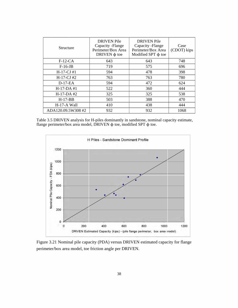
A
Table 3flange p
Figure 3
perimet
Structu
F-12-CF-16-J
H-17-CH-17-CD-17-E
H-17-DAH-17-DA
H-17-BH-17-A
ADA120.09.5
.5 DRIVENperimeter/bo
3.21 Nomin
ter/box area
ure
CA JB
CJ #1 CJ #2 EA A #1 A #2 BB Wall 5W308 #2
N analysis forox area mode
nal pile capa
a model, toe
DRIVECapacity
PerimeterDRIVE
647597659523250493
r H-piles doel, DRIVEN
acity (PDA)
e friction an
38
EN Pile y -Flange r/Box Area EN ϕ toe
43 19 94 63 94 22 25 03 10 32
minantly in
N ϕ toe, mod
) versus DR
gle per DRI
DRIVECapacity
PerimeterModified
645474332349
sandstone, ndified SPT ϕ
RIVEN estim
IVEN.
EN Pile y -Flange r/Box Area SPT ϕ toe
43 75 78 63 72 60 25 88 38 32
nominal capϕ toe.
mated capac
Case (CDOT) k
748 696 398 780 624 444 538 470 444 1068
pacity estima
city for flan
kips
ate,
nge

Figure 3
perimet
A Table 3flange p
3.22 Nomin
ter/box area
Structu
F-12-CF-16-J
H-17-CH-17-CD-17-E
H-17-DAH-17-DA
H-17-BH-17-A
ADA120.09.5
.6 DRIVENperimeter/tip
nal pile capa
a model, toe
ure
CA JB
CJ #1 CJ #2 EA A #1 A #2 BB Wall 5W308 #2
N analysis forp area model
acity (PDA)
e friction an
DRIVECapacity
PerimeterDRIVE
12159121010510733
r H-piles dol, DRIVEN
39
) versus DR
gle per SPT
EN Pile y -Flange r/Tip Area
EN ϕ toe
21 57
92 22 06 02
57 00
76 38
minantly in ϕ toe, modi
RIVEN estim
T
DRIVECapacity
PerimeterModified
121712895863
sandstone, nified SPT ϕ
mated capac
EN Pile y -Flange r/Tip Area SPT ϕ toe
21 33 76 22 89 90 57 83 68 38
nominal captoe.
city for flan
Case (CDOT) k
748 696 398 780 624 444 538 470 444 1068
pacity estima
nge
kips
ate,

Figure 3
perimet
Figure 3
perimet
3.23 Nomin
ter/tip area m
3.24 Nomin
ter/tip area m
nal pile capa
model, toe f
nal pile capa
model, toe f
acity (PDA)
friction ang
acity (PDA)
friction ang
40
) versus DR
gle per DRIV
) versus DR
gle per SPT.
RIVEN estim
VEN.
RIVEN estim
mated capac
mated capac
city for flan
city for flan
nge
nge

AD Table 3perimete
Figure 3
perimet
Structu
F-12-CF-16-JB
H-17-CJH-17-CJD-17-E
H-17-DAH-17-DA
H-17-BH-17-A W
DA120.09.5W
.7 DRIVENer/box area
3.25 Nomin
ter/box area
ure
CA B
J #1 J #2 EA A #1 A #2 BB Wall W308 #2
N analysis formodel, DRI
nal pile capa
a model, toe
DRIVECapacity
Perimeter/BDRIVEN
677662796142335355
115
r H-piles doIVEN ϕ toe,
acity (PDA)
e friction an
41
EN Pile y -Box Box Area N ϕ toe
75 66 21 91 7
29 36 34 53 52
minantly in , modified S
) versus DR
gle per DRI
DRIVECapacit
Perimeter/Modified
67624979493733414611
sandstone, nSPT ϕ toe.
RIVEN estim
IVEN.
EN Pile ty -Box /Box Area SPT ϕ toe
75 21 94 91 94 79 36 18 63 52
nominal cap
mated capac
Case (CDkips
748 696 398 780 624 444 538 470 444 1068
pacity estima
city for box
OT)
ate, box

Figure 3
perimet
AD Table 3perimete
3.26 Nomin
ter/box area
Structu
F-12-CF-16-JB
H-17-CJH-17-CJD-17-E
H-17-DAH-17-DA
H-17-BH-17-A W
DA120.09.5W
.8 DRIVENer/tip area m
nal pile capa
a model, toe
ure
CA B
J #1 J #2 EA A #1 A #2 BB Wall W308 #2
N analysis formodel, DRIV
acity (PDA)
e friction an
DRIVECapacity
Perimeter/DRIVEN
18241217151678161576
r H-piles doVEN ϕ toe, m
42
) versus DR
gle per SPT
EN Pile y -Total /Tip Area N ϕ toe
82 48 25 76 51 62 8 61 51 68
ominantly in modified SP
RIVEN estim
T.
DRIVECapacit
PerimeterModified
1822101713147141076
sandstone, PT ϕ toe.
mated capac
EN Pile ty -Total r/Tip Area SPT ϕ toe
82 24 09 76 33 49
78 44 03 68
nominal cap
city for box
Case (CDkips
748 696 398 780 624 444 538 470 444 1068
pacity estim
OT)
ate, total

Figure 3
perimet
Figure 3
perimet
3.27 Nomin
ter/tip area m
3.28 Nomin
ter/tip area m
nal pile capa
model, toe f
nal pile capa
model, toe f
acity (PDA)
friction ang
acity (PDA)
friction ang
43
) versus DR
gle per DRIV
) versus DR
gle per SPT.
RIVEN estim
VEN.
RIVEN estim
mated capac
mated capac
city for total
city for total
l
l

44
3.3.3 DRIVEN Capacity Estimates for H-piles and Pipe Piles in Sand, Clay, Gravel
Data is largely from the Eastern Plains with a few sites in mountain valleys. Three sites in the
mountains and one site in the Front Range are dominantly gravel or gravelly sand. The
remaining fourteen sites are on the Eastern Plains consisting dominantly of poorly sorted
sand or silty-clayey sand with lenses of gravelly-sand, gravel and clay. H-piles and pipe piles
are commonly closed-end piles with welded end plates to increase end bearing resistance.
Some H-piles had no end plates if driven in sand with cobbles and small boulders, or if very
hard calcareous-clay sections or gravel layers had to be penetrated at shallower depths to
achieve deeper penetration. Unless a strong bearing stratum such as dense gravel is
encountered, pile lengths are typically longer than for clay shale, shale and sandstone.
General types of soil profiles that typically provide capacity are presented. Thick intervals of
loose to medium dense sand (possibly silty to clayey with interspersed clay lenses) that lack
stronger soil intervals are common in areas on the Eastern Plains and provide only moderate
pile capacity. If gravel beds thick enough to provide higher end-bearing capacity occur within
the sand section or form thick deposits which underlie the sand, pile capacity can be
increased with short penetration into gravel. Thick beds of very hard (SPT > 50), calcareous
clay may also increase bearing capacity. More common in mountain valleys, thick deposits of
gravel and sandy gravel provide very high resistance in H-piles with no end plates.
The following friction angles were used for gravels and gravelly sands: 1) sub-angular
gravels with cobbles (GP-GW), small boulders, admixed sand, end bearing friction 43°, skin
friction 40°, 2) sub-rounded to rounded, small-medium gravel with sand or gravelly sand
(GP-SP, GW-SW), end bearing friction 38°, skin friction 34°, 3) sub-rounded to rounded,
small-medium gravel, slightly silty or clayey with sand or gravelly sand (GC-GM with
SC-SM), end bearing friction 37°, skin friction 34°, lower friction angles with increasing
clay-silt content, 4) typical sub-angular to sub-rounded sand that may be slightly clayey or
silty (SP, SW, SP-SC, SP-SM), end bearing friction as calculated by DRIVEN with a
maximum value of 36°, skin friction 32° maximum or lower value by DRIVEN, lower
friction angles with increasing clay-silt content.
Lower skin friction angles were used to account for loosening of sand along the pile shaft
during driving and to compensate for the effect of increasing unit shaft resistance inherent in
DRIVEN. The pile box area was used for H-piles with end plates and for H-piles with open
sections. For pipe piles, DRIVEN uses pile perimeter surface area with an option for open or
closed end pipe. DRIVEN static capacity estimation of pile capacity for the end of drive
condition with zero setup time used the following parameters: pile box area, box perimeter

45
for H-piles, full perimeter and closed end for pipe piles, adhesion coefficient of 1.0 for moist,
normally consolidated clay, adhesion coefficient of 0.5 for overconsolidated or desiccated
clay, 50 percent driving strength loss for clay and zero percent driving strength loss for sand.
Two models of pile resistance were considered:
1. Box perimeter-box area for H-piles with pile perimeter-closed end for pipe piles
2. Flange perimeter-box area for H-piles with 50% perimeter-closed for pipe piles.
Results of analyses are summarized in Table 3.9
From the Driven result, the box perimeter/box area model for H-piles and pile perimeter,
closed end model for pile piles has the nominal capacity closer to the PDA (Case) testing from
CDOT.
Structure
DRIVEN Pile Capacity -Box Perimeter, Box Area for H-piles; Pile Perimeter, Closed End for Pipe Piles
DRIVEN Pile Capacity -Flange Perimeter, Box Area for H-piles; 50% Pile Perimeter, Closed
End for Pipe Piles
Case (CDOT) kips
C-21-BO 286 153 323 C-21-BN 400 319 311 C-21-BV 262 141 382
C-22-BU #1 387 313 366 C-22-BU #2 387 313 388
D-20-K 372 234 335 D-20-K #1 470 257 410 D-20-K #2 305 200 322 D-20-K #4 295 207 312 D-20-K #5 270 188 327 B-23-AW 309 202 324
B-27-J 393 240 440 B-27-J #1 537 319 464 B-27-J #2 444 286 399
I-16-AE #1 329 256 354 I-16-AE #2 253 200 316
E-12-I 671 619 800 ADA-120-008.8W
306 175 107 190
Table 3.9 DRIVEN analysis for piles dominantly in sand, gravel or clay.

Figure 3
perimet
3.29 Nomin
ter-box area
nal pile capa
a for H-piles
acity (PDA)
s, pile perim
46
) versus DR
meter-closed
RIVEN estim
d end for pip
mated capac
pe piles
city for box

Figure 3
perimet
3.4 Sum
The cap
with cla
0.70, wi
with san
of pile c
capaciti
to overe
the futu
caution
Pile Type
CDO
H IM
H BR
H STA
H BR
H BR
3.30 Nomin
ter-box area
mmary Cap
pacities of H
ay shale and
ith sand ston
nd, clay and
capacities, C
ies are high
estimate the
ure to see if
.
T
OT Reference
M-0251-166
R 0251-162
A 0091-016
R 0402-056
R 0402-056
nal pile capa
a for H-piles
pacity of th
H-piles usin
d shale usin
ne using the
d gravel usin
Case capaci
er than DRI
e pile capaci
this is indee
able 3.10. CA
Region
II
II
I
III
III
acity (PDA)
s, 50% perim
he H-piles fr
ng DRIVEN
g the box p
box perime
ng box peri
ities are hig
IVEN capac
ity. This ob
ed the case.
APWAP, Ca
Location
P-18-BY Abu
K-18-HA
F-12-CA
D-11-A-1
D-11-A-2
47
) versus DR
meter-close
from DRIV
N 1.1 from C
erimeter/bo
eter/box are
imeter/box a
her than CA
cities in 17
bservation h
. If so, the C
ase (CDOT)
n Pile
ut #8 12 x
A 12 x
A 12 x
1 12 x
2 12 x
RIVEN estim
ed for pipe p
VEN 1.1
CDOT proje
ox area mod
ea model wi
area model
APWAP cap
cases. In su
as to be che
Case capacit
and DRIVEN
SizePile
Depthft
x 74 26
x 74 20
x 74 23
x 74 71.5
x 74 68
mated capac
piles.
ect are show
del with adh
ith toe fricti
for H-piles
pacities in 2
um, the Case
ecked with t
ty would ha
N 1.1 Capaci
CAPWAPKips
742.3
943.6
570
548.8
469.1
city for flan
wed in Table
hesion factor
on angle pe
. Out of the
22 cases, an
e capacities
the load res
ave to be us
ity Case
(CDOT) Kips
D
796
927
748
743
672
nge
e 3.10,
r α =
er SPT,
24 sets
nd Case
s seem
ults in
ed with
Driven 1.1 Kips
702*
604*
675**
766*
614*

48
H NH 2873-114 IV C-16-BX 12 x 74 10 394.3 468 420*
H NH 2873-114 IV C-16-CK 12 x 74 56 362.9 510 409* H NH 2873-114 IV C-16-BC 12 x 74 56 495 598 589* H STA 012A-039 II P-18-AX 12 x 74 25 680.3 734 752* H NH 0505-037 II L-25-D 12 x 74 26.5 290.3 520 505* H STU C120-007 VI ADA 120-09-1 12 x 84 35.5 608.2 848 629*
H STU C120-007 VI ADA 120-09-2R 12 x 84 55.5 1480.9 1068 1244* H STU C120-007 VI ADA 120-08.8w306-1 12 x 84 50.5 578 572 457* H STU C120-007 VI ADA 120-07.9e305 12 x 84 46.5 381.1 586 533* H STU C120-007 VI ADA 120-08.8w306 12 x 84 24 127.6 186 175*** H STU C120-007 VI COMC-12-0.2-01A 12 x 84 46 566.3 548 485* H STU M240-081 II H-17-CJ-2 14 x 89 26 594 780 791** H STU M240-081 II H-17-CJ-1 14 x 89 18 289.6 398 494** H BR 0062-013 IV D-20-K-1 12 x 53 78 239.8 410 470*** H BR 0062-013 IV D-20-K 12 x 53 64 224.3 335 372*** H BR 0062-013 IV D-20-K-5 12 x 53 50 220.8 327 270*** H BR 0062-013 IV D-20-K-2 12 x 53 48 250.6 322 305*** H BR 0062-013 IV D-20-K-4 12 x 53 50 236 312 295*** H BR 0521-162 II K-18-GQ 12 x 74 30 518.4 522 764* * H-pile dominantly in clay shale and shale ** H-piles dominantly in Sand stone ***H-pile dominantly in sand, gravel or clay

49
4.0 WAVE EQUATION ANALYSIS
4.1 Introduction Wave equation analysis of pile driving is based on the solution of the partially differential equation for propagation of wave along the prismatic rod (pile) accounting for the soil-pile interaction ( Hannigan et al., 1998). The wave equation approach was developed by Smith (1960). Subsequent work by numerous researchers in the 1960’s and 1970’s lead to a number of computer programs. The Texas Transportation Institute developed one of the first programs in an attempt to reduce concrete pile damage. FHWA sponsored development of the Texas Transportation Institute Program and the WEAP (wave equation analysis program) program (Goble and Rausche, 1976). The WEAP program has been updated several times under FHWA sponsorship and its current form is known as GRLWEAP (Goble, Rausche, Likins and Associates, Inc., 1996). GRLWEAP has been accepted by numerous public agencies and the FHWA in the pre-installation analysis of driven piles designed for the evaluation of dynamic pile stresses and driving resistance using a selected pile driving hammer, pile resistance including side shear and end bearing components under given subsoil conditions.
Before the discussion of GRLWEAP analysis, the following definitions (Rausche et al., 1992) of parameters involved are presented:
1. Static soil resistance, Rs, is a function of the relative displacement between pile and soil and is assumed to be present during static and dynamic loading. While Rs is a function of displacement and varies with time, Ru, the ultimate soil resistance, is constant. 2. The damping resistance, Rd, is the portion of soil resistance, not present during static load application. It varies with time and is commonly thought to be related to pile velocity. 3. The total resistance during pile driving, Rt, is called the dynamic resistance. It is the sum of static and damping resistances. Under static loads, damping resistance is zero and total resistance equals the static resistance. 4. The slip layer is a zone along the pile-soil interface where the relative motion between pile wall and soil mass occurs.
4.2 Selection of Input Parameters for GRLWEAP Analyses Energy delivered to the pile head is a critical parameter in wave equation analysis. GRLWEAP incorporates a mathematical model of combustion chamber force that is introduced between the hammer ram and the anvil together with the pile helmet and pile cushion characteristics to calculate the energy delivered at the pile head to advance the pile

(Figure elasto-pdampincan be mGRLWwith thediesel h
Figure 4equation
4.1). Smithplastic sprinng resistancemeasured inEAP re-anae PDA meahammer syst
4.1 GRLWEn model, (C
h (1960) repng to represee. The energn the field aalysis was tosurement oftem perform
EAP prograC) the soil re
presented thent static regy deliveredas a compono match, wif Enthru. GRmance. As th
am componeesistance m
50
he forces exesistance andd to the pilenent of PDAithin 10 percRLWEAP hhe exact det
ents: (A) thmodel (Goble
erted in the d a quasi line head is termA analyses. Tcent, the GRhas a large rtails of ham
e system to e and Rausc
pile-soil innear dashpomed EnthruThe initial sRLWEAP crange of inp
mmer system
be analyzeche, 1976).
nterface by aot to model tu (kip-ft). Enstep in the calculated Eput options m performan
d, (B) the w
an the nthru
Enthru for
nce are
wave

51
unknown, the following parameters were used: hammer efficiency set at 80 percent for all hammers, the combustion pressure varies as a percentage of the rated value to match the GRLWEAP calculated Enthru to the PDA measurement, diesel hammer combustion pressure varies over hammer life as compression rings wore out or replaced, and the helmet and cushion materials selected in accordance with manufacturer specifications. The soil resistance profile from DRIVEN was converted to a GRLWEAP input file using the driveability option in DRIVEN. The pile capacity from DRIVEN was adjusted in RLWEAP, where necessary, using the pile strength gain/loss option to within 10 percent of the PDA nominal value. The GRLWEAP soil resistance model requires values for soil quake and soil damping. Soil quake is the displacement at which the soil changes from elastic to plastic behavior with the application of maximum force (Figure 4.1c). In the Smith damping model, the dynamic soil resistance is proportional to a damping factor times the pile velocity times the assigned static resistance for an interval. Shaft quakes, toe quakes, shaft damping and toe damping are the four basic Smith soil model parameters that are used to describe the dynamic soil behavior in GRLWEAP. Analyses used the recommended (GRL, 2005) default values for soil types (Table 4.1, Table 4.2).
Soil Type Damping Factor s/ft Damping Factor s/m
Shaft Damping
Non-cohesive soils 0.05 0.16
Cohesive soils 0.20 0.65
Toe damping In all soil types 0.15 0.50
Table 4.1 Recommended damping values for impact driven piles GRLWEAP.

52
Soil Type Pile Type or Size Quake (in) Quake (mm)
Shaft Quake All soil types All Types 0.10, 2.5
Toe Quake All soil types, soft RockNon-displacement piles i.e. driving unplugged
0.10. 2.5
Very dense or hard soilsDisplacement Piles of diameter or width D
D/120 D/120
Loose or soft soils Displacement Piles of diameter or width D
D/60 D/60
Hard Rock All Types 0.04, 1.0
Table 4.2 Recommended quake values for impact driven piles GRLWEAP.
4.3 Results of GRLWEAP Analyses 4.3.1 GRLWEAP Analyses of Transmitted EnergyEnthru calculated by GRLWEAP closely approximated, within 10 percent, the PDA measured value (Figure 4.2). For two sites with low Enthru values, GRLWEAP yielded higher energy values for hammer performance. A hammer system efficiency of 80 percent with a varying percentage of the rated combustion pressure in GRLWEAP made a satisfactory overall estimate of the energy delivered to the pile. The percentage of rated combustion pressure varied from 65 to 110 percent and reflects the range of hammer performance. For the suite of hammers, a value between 70 and 90 percent of rated combustion pressure was most frequent (Figure 4.2).

53
Figure 4.2 Correlation between measured and calculated Enthru values.
Figure 4.3 Range of rated combustion pressure percentage used in GRLWEAP to match PDA Enthru values
H Piles, Pipe Piles
0
10
20
30
40
50
0 10 20 30 40 50
Enthru (kip-ft) Calculated by GRLWEAP
Ent
hru
(kip
-ft) M
easu
red
by P
DA
Sand,Gravel,ClaySandstoneClay Shale, Shale
0
2
4
6
8
10
12
14
16
65 70 75 80 85 90 95 100 105
Rated Combuston Pressure % GRLWEAP
Num
ber o
f Pile
s

54
4.3.2 GRLWEAP Analysis of Compressive Stress With input of a soil resistance profile, hammer type-hammer performance (expressed in calculated Enthru), and pile type, GRLWEAP calculates tensile and compressive stresses developed in a pile during driving. In steel piles, tensile stresses are only a fraction of the compressive stress and typically are not of concern in Colorado rocks, where piles are socketed. A principal use of wave equation analysis is to estimate pile stresses before pile installation to determine if the pile can be driven without overstressing, to a desired resistance using a specific hammer. Compressive stress in steel piles during driving is limited, per AASHTO standard specifications, to 90 percent of the steel yield strength. For grade 50 steel piles, the maximum allowable compressive stress is 45 ksi. Estimates of pile compressive stresses calculated by GRLWEAP are termed “conservative,” if they overestimated compressive stress compared to the PDA measurement. Highly overconservative estimates of compressive stress might predict that pile damage would occur, whereas the pile could be driven with no damage. GRLWEAP estimates of pile compressive stress are summarized in Table 4.3.
Model Correlation Coefficient
WEAP Mean Difference from PDA /Range
Conservative % of analysis – degree
Clay Shale, Shale – H-pile, Pipe Pile
0.74
+1 ksi (+19 to -13)
56%-Low/High
Sandstone - H-pile
0.70
+6 ksi (0 to +14)
100%-Low/High
Sand, Gravel, Clay - H-pile, Pipe Pile
0.42
-2 ksi (+8 to -6)
28% -Low
Table 4.3 Summary of GRLWEAP compressive stress estimates in piles compared to PDA compressive stress measurements. For H-piles and 2 open-end pipe piles driven in clay shale and shale, GRLWEAP stresses showed, in general, a satisfactory agreement with the PDA measured stress (Figure 4.4), although WEAP values were frequently higher than PDA values (+19 to -13 ksi of PDA stresses), particularly when piles were driven into very hard to extremely hard partially cemented Pierre shale. Fifty-six percent of GRLWEAP values were conservative with four piles with highly conservative pile stresses of 12 to 19 ksi higher than PDA values, of which three exceeds 45 ksi in the range of 48 to 58 ksi. Excluding the 3 piles with calculated stress higher than 45ksi, GRLWEAP pile stresses of piles in clay shale and shale could reasonably serve as an indicator for safety of piles during the dynamic pile driving.

55
For H-piles driven in uncemented and partially cemented sandstone, calculated compressive stresses showed a satisfactory match with the PDA measured stress (Figure 4.5). GRLWEAP values ranged from 0 to +14 ksi of the PDA measurement. One hundred percent of GRLWEAP values were conservative. Two piles had highly conservative estimates of pile stress being 14 ksi higher than PDA values. However, none of estimated pile stresses exceeded 42 ksi and were overly conservative. GRLWEAP estimates of pile stress in sandstone served as a reasonable indicator of potential pile damage during driving.
Figure 4.4 Correlation between measured and calculated compressive stress for piles in clay shale, shale.
H Piles, Pipe Piles in Clay Shale, Shale
0
10
20
30
40
50
60
70
0 10 20 30 40 50 60 70
Maximum Compressive Pile Stress Calculated by GRLWEAP - (ksi)
Max
imum
Com
pres
ssiv
e P
ile S
tress
by
PD
A -
(ksi
)

56
Figure 4.5 Correlation between measured and calculated compressive stress for H-piles in sandstone. For H-piles and pipe piles driven in sand, gravel, and clay, calculated compressive stress showed a satisfactory agreement with the PDA measured stress (Figure 4.6). Measured pile stresses were in a fairly narrow range of 23 to 31 ksi. GRLWEAP values ranged from +8 to -6 ksi of the PDA measurement. Estimated pile stress only exceeded 30 ksi once. Twenty- six percent of GRLWEAP values were conservative. Most stress estimates from GRLWEAP were non-conservative with stresses smaller than PDA measured stresses by 3 to 5 ksi with practically no effect on the judging pile damage. GRLWEAP can provide satisfactory estimates of pile stress, if the soil resistance distribution and hammer performance parameters are reasonably known. For evaluation of pile stress prior to driving, hammer performance is unknown. The soil resistance can be estimated using DRIVEN. Default values for soil quake and damping from GRLWEAP are suggested. A value of 80 percent hammer efficiency is recommended. As shown in Figure 4.2, percentage of rated combustion pressure is most frequently in the 70 to 90 percent range. Two GRLWEAP analyses to estimate pile stress prior to driving are recommended using 70 and 90 percent of rated combustion pressure. If the current performance of a given hammer can be estimated, the range of combustion pressure could be extended higher or lower.
H Piles in Sandstone
0
10
20
30
40
50
0 10 20 30 40 50
Maximum Compressive Pile Stress by GRLWEAP - (ksi)
Max
imum
Com
pres
sive
Pile
Stre
ss b
y PD
A - (
ksi)

57
Three observations from GRLWEAP analyses are: 1) If both lower and upper bound analyses yield pile stress less than 45 ksi, the hammer and pile section area are acceptable; 2) If both lower and upper bound values exceed 45 ksi, the magnitude of the stress estimates requires further evaluation; 3) Dynamic pile stresses of 45 to 50 ksi can correspond to lower field stresses given the tendency for conservative stress estimates in weak rock; 4) GRLWEAP calculated stresses in 50-60 ksi range or higher indicate a different hammer or pile section is likely needed; 5) If the lower bound stress estimate is less than 45 ksi and the upper bound estimate is in the 45 to 50 ksi range, the hammer and pile section are likely acceptable subject to PDA verification. DRIVEN analysis provides input file for pre-installation GRLWEAP analysis; the driving pile stresses should be verified with the PDA measured stresses; GRLWEAP re-analysis and comparison with PDA measured stresses are recommended before the installation of production piles and potential dynamic compressive stresses during pile driving.
Figure 4.6 Correlation between measured and calculated compressive stress for piles in sand, gravel, clay. 4.3.3 GRLWEAP Analyses of Driving Resistance In the compressive stress estimate, GRLWEAP calculates the displacement (permanent set) of the pile toe. The inverse of the permanent set is the driving resistance in blows per foot,
H Piles, Pipe Piles in Sand, Gravel, Clay
0
10
20
30
40
0 10 20 30 40
Maximum Compressive Pile Stress by GRLWEAP - (ksi)
Max
imum
Com
pres
sive
Pile
Stre
ss b
y P
DA
-(k
si)
58
which is related to the nominal capacity of pile. Estimation of driving resistance prior to driving provides criteria for evaluating if a hammer has enough energy to drive a pile at a reasonable rate to the required capacity. Consider the following example for an H 12x74 piles driven through 15 feet of loose sand into clay shale. Side resistance in clay shale is 27 kips per foot of penetration with an end bearing resistance of 120 kips. Thus, for a 10 foot rock penetration, estimated nominal pile capacity is 10 ft x 27 kips/ft plus 120 kips equals 390 kips for end of drive condition. GRLWEAP analyses to estimate driving resistance used two hammers; Delmag D19-42 with a rated energy of 43,240 ft-lb and Delmag D 12-32 with a rated energy of 31,330 ft-lb. For the Delmag D 19-42 hammer, GRLWEAP analysis indicated that the pile could be driven to the desired resistance of 390 kips with an estimated maximum blow count of 120 blows per foot (Figure 4.7) with a reasonable driving rate. For the Delmag D 12-32 hammer (lower energy), GRLWEAP analysis (Figure 4.8) indicated a sizeable increase in blow count at about 250 kips pile resistance and hard to impractical driving increasing from 100 to over 200 blows per foot at the required resistance of 390 kips. The rate of increase in pile resistance with depth was much lower than the rate of increase in blow count. Thus, Delmag D 12-32 hammer cannot transmit enough energy to the pile section embedded in the clay shale and advance the pile at a practical rate.

59
Figure 4.7 GRLWEAP drivability model for Delmag D 19-42 hammer in example profile.
CO Dept of Transp - Univ of Colorado Sep 11 2010
: 09/11/2010 : Gain/Loss 1 at Shaft and Toe 1.000 / 1.000GRLWEAP(TM) Version 2005D
epth
(ft)
0 50 100 150 200
4
8
12
16
20
24
28
32
36
40
Blow Count (blows/ft)
Dep
th (f
t)
0 200 400 600 800
4
8
12
16
20
24
28
32
36
40
Ult. Capacity (kips)
0 10 20 30 40
4
8
12
16
20
24
28
32
36
40
Tension (ksi)
0 10 20 30 40
4
8
12
16
20
24
28
32
36
40
Comp. Stress (ksi)
0.0 2.0 4.0 6.0 8.0
4
8
12
16
20
24
28
32
36
40
Stroke (ft)
0.0 5.0 10.0 15.0 20.0
4
8
12
16
20
24
28
32
36
40
ENTHRU (kips-ft)
Sand
Clay Shale

60
Figure 4.8 GRLWEAP drivability model Delmag D 12-32 hammer in example profile. GRLWEAP analyses and driving records show that driving resistance typically increases in a nonlinear manner as the ratio of hammer energy to pile capacity decreases during driving. If the available hammer energy is not sufficient to maintain the rate of pile advance, penetration can rapidly decrease producing very high blows with little penetration as pile refusal occurs. The ability of a hammer to advance a pile to achieve higher resistance is determined by the rate of increase of driving resistance with depth relative to the rate of increase in pile capacity with depth. The wave equation shows this relationship as the slope of blow count and pile capacity plots with depth. Three examples from project sites are discussed below. Site 1 is from structure B-23-AW, Abutment #1, along US 6 north of Atwood in Logan County. A 12.75 inch closed end pipe pile was driven 65 feet by an APE D19-42 hammer (Figure 4.9). The section consists of sandy clay overlying sand and gravelly sand. Most pile capacity is developed in medium dense, gravelly sand below 40 feet. A GRLWEAP model of pile
CO Dept of Transp - Univ of Colorado Sep 11 2010
: 09/11/2010 : Gain/Loss 1 at Shaft and Toe 1.000 / 1.000GRLWEAP(TM) Version 2005D
epth
(ft)
0 50 100 150 200
4
8
12
16
20
24
28
32
36
40
Blow Count (blows/ft)
Dep
th (f
t)
0 200 400 600 800
4
8
12
16
20
24
28
32
36
40
Ult. Capacity (kips)
0 10 20 30 40
4
8
12
16
20
24
28
32
36
40
Tension (ksi)
0 10 20 30 40
4
8
12
16
20
24
28
32
36
40
Comp. Stress (ksi)
0.0 2.0 4.0 6.0 8.0
4
8
12
16
20
24
28
32
36
40
Stroke (ft)
0.0 4.0 8.0 12.0 16.0
4
8
12
16
20
24
28
32
36
40
ENTHRU (kips-ft)
Sand
Clay Shale

61
derivability shows that driving resistance in blows per foot (solid line on left graph) is increasing at only a slightly greater rate than the rate of capacity increase (dashed line on left graph) indicating easy driving conditions for the hammer with 7 feet ram stroke for a pile capacity of 325 kips. The hammer has sufficient energy to drive the pile deeper. Compressive stress in the pile (center graph) shows a progressive increase with depth to 23 ksi well below the 45 ksi allowable maxima. Comparison between PDA measurements and (GRLWEAP) model are: pile capacity 324 kips (307 kips), compressive stress 25.7 ksi (22.4 ksi), hammer energy 16.0 kip-ft (16.5 kip-ft), driving resistance 40 blows per foot (57 blows per foot).
Figure 4.9 WEAP drivability model for structure B-23-AW, Abutment #1.
Site 2 is from structure C-16-BC, Abutment #1, along US 287/Berthoud Bypass in Weld County. A 12 x74 H-pile was driven 56 feet by a Delmag D30-32 hammer (Figure 4.10).
CO Dept of Transp - Univ of Colorado Sep 12 2010
: 09/12/2008 : Gain/Loss 1 at Shaft and Toe 0.400 / 1.000GRLWEAP(TM) Version 2005
Dep
th (f
t)
0 20 40 60 80
10
20
30
40
50
60
70
80
90
100
Blow Count (blows/ft)
Dep
th (f
t)
0 100 200 300 400
10
20
30
40
50
60
70
80
90
100
Ult. Capacity (kips)
0 10 20 30 40
10
20
30
40
50
60
70
80
90
100
Tension (ksi)
0 10 20 30 40
10
20
30
40
50
60
70
80
90
100
Comp. Stress (ksi)
0 4 8 12 16
10
20
30
40
50
60
70
80
90
100
Stroke (ft)
0 5 10 15 20
10
20
30
40
50
60
70
80
90
100
ENTHRU (kips-ft)
GRAVELLY SAND
SANDY CLAY
62
The section consists of 44 feet stiff clay overlying medium hard, hard, and very hard clay shale. Most capacity is developed in the 12 feet of clay shale penetrated by the pile. A GRLWEAP model of pile derivability shows that driving resistance in blows per foot (solid line on left graph) increases at a greater rate than the rate of capacity increase (dashed line on left graph). The driving resistance continues to increase without much additional penetration, which indicates the onset of hard driving conditions. The hammer, with 7 to 8 foot ram stroke, does not have sufficient energy to readily drive the pile deeper. Compressive stress in the pile (center graph) shows a progressive increase with depth to 28 ksi well below the 45 ksi allowable maxima. Comparison between PDA measurements and (GRLWEAP) model are: pile capacity 598 kips (556 kips), compressive stress 29.4 ksi (31.6 ksi), hammer energy 29.4 kip-ft (29.2 kip-ft), driving resistance 120 blows per foot (149 blows per foot). Site 3 is from structure F-18-BK, Pier #13, along US 36 in Adams County. A 24 inch closed-end pipe pile was driven 16 feet by a Delmag D30-32 hammer (Figure 4.11). The section consists of 22 feet medium dense to dense gravelly sand and 22-foot stiff clay, overlying medium hard, hard, and very hard clay shale. The design specified that the closed-end pipe pile be driven through the overburden soil into clay shale. Due to refusal in sand at 16 feet, the end plate was removed and the pile was driven as an open-end pipe pile into clay shale. This is the only site that contains any data on a large diameter pipe pile. The sand is coarse-grained, gravelly with medium dense to dense SPT blows. With corrections for auto-hammer energy and overburden stress, DRIVEN calculated an effective friction angle of 39° for the lower portion of the gravelly sand. Initial GRLWEAP analyses used: default sand parameters for soil quake and damping, 39°friction angle for end bearing, 34° friction angle for side resistance and 80 percent hammer efficiency with 85 percent combustion pressure. Exact hammer parameters are unknown, but the hammer performed in a satisfactory manner. The GRLWEAP analyses indicated that the hammer likely could have safely driven the 24 inch pipe pile through the gravelly sand interval. GRLWEAP estimated 80 blows per foot at 16 feet of penetration increasing to 120 blows per foot near the base of the sand with 20 feet of penetration (Figure 4.12). Nominal pile resistance at 16 feet was estimated at 580 kips by DRIVEN. GRLWEAP tends to overestimate blow counts at pile data sites in sand and sandstone and somewhat high blow counts in GRLWEAP analyses may not indicate pile refusal. Although the driving rate could be slow, the pile should have advanced through the sand based on the soil resistance model. The empirical relationships used in DRIVEN to estimate pile resistance in this report are based mainly on analyses of 12 inch H-piles. Driving low displacement H-piles in sand likely has a different effect on soil resistance than does large, high displacement pipe piles (Conduto. 2001), although quantification is difficult. Driving a large diameter displacement pile through a medium dense to dense gravelly sand
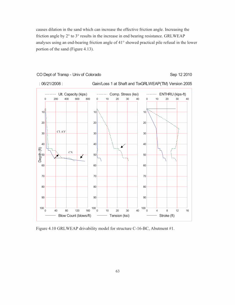
63
causes dilation in the sand which can increase the effective friction angle. Increasing the friction angle by 2° to 3° results in the increase in end bearing resistance. GRLWEAP analyses using an end-bearing friction angle of 41° showed practical pile refusal in the lower portion of the sand (Figure 4.13).
Figure 4.10 GRLWEAP drivability model for structure C-16-BC, Abutment #1.
CO Dept of Transp - Univ of Colorado Sep 12 2010
: 06/21/2008 : Gain/Loss 1 at Shaft and Toe 0.400 / 1.000GRLWEAP(TM) Version 2005
Dep
th (f
t)
0 40 80 120 160
10
20
30
40
50
60
70
80
90
100
Blow Count (blows/ft)
Dep
th (f
t)
0 200 400 600 800
10
20
30
40
50
60
70
80
90
100
Ult. Capacity (kips)
0 10 20 30 40
10
20
30
40
50
60
70
80
90
100
Tension (ksi)
0 10 20 30 40
10
20
30
40
50
60
70
80
90
100
Comp. Stress (ksi)
0 4 8 12 16
10
20
30
40
50
60
70
80
90
100
Stroke (ft)
0 10 20 30 40
10
20
30
40
50
60
70
80
90
100
ENTHRU (kips-ft)
CLAY
CS

Figure 44.11 Boringg log profilee of 24 inch
64
closed-endd pipe pile wwith refusal at 16 feet.

65
Figure 4.12 Initial GRLWEAP drivability model for structure F-18-BK, Pier #3.
CO Dept of Transp - Univ of Colorado Sep 13 2010
: 09/20/2010 : Gain/Loss 1 at Shaft and Toe 1.000 / 1.000GRLWEAP(TM) Version 2005
Dep
th (f
t)
0 40 80 120 160
4
8
12
16
20
24
28
32
36
40
Blow Count (blows/ft)
Dep
th (f
t)
0 200 400 600 800
4
8
12
16
20
24
28
32
36
40
Ult. Capacity (kips)
0 10 20 30 40
4
8
12
16
20
24
28
32
36
40
Tension (ksi)
0 10 20 30 40
4
8
12
16
20
24
28
32
36
40
Comp. Stress (ksi)
0.0 2.0 4.0 6.0 8.0
4
8
12
16
20
24
28
32
36
40
Stroke (ft)
0.0 10.0 20.0 30.0 40.0
4
8
12
16
20
24
28
32
36
40
ENTHRU (kips-ft)
Sand
Gravelly Sand

66
Figure 4.13 Modified GRLWEAP drivability model for structure F-18-BK, Pier #3.
GRLWEAP estimated 240 blows per foot at 16 feet of penetration increasing to over 400 blows per foot near the base of the sand with 20 feet of penetration. Nominal pile resistance at 16 feet was estimated at 820 kips by DRIVEN using a friction angle of 41°. Use of large diameter pipe piles with closed end is limited by difficulty in driving through dense gravel layers and hard calcareous clays common in soil profiles along the Front Range. The force in a pile, with no resistance effects, when hit by a hammer is equal to the particle velocity caused by the stress wave traveling through the pile times the pile impedance (Rausche et al., 1985). Pile impedance is equal to EA/C: where E is the elastic modulus, A is the pile cross section area, and C is wave speed. In application, the sectional area of large diameter pipe piles is low compared to the high end bearing resistance mobilized by a
CO Dept of Transp - Univ of Colorado Sep 13 2010
: 09/20/2010 : Gain/Loss 1 at Shaft and Toe 1.000 / 1.000GRLWEAP(TM) Version 2005D
epth
(ft)
0 100 200 300 400
4
8
12
16
20
24
28
32
36
40
Blow Count (blows/ft)
Dep
th (f
t)
0 400 800 1200 1600
4
8
12
16
20
24
28
32
36
40
Ult. Capacity (kips)
0 10 20 30 40
4
8
12
16
20
24
28
32
36
40
Tension (ksi)
0 10 20 30 40
4
8
12
16
20
24
28
32
36
40
Comp. Stress (ksi)
0 4 8 12 16
4
8
12
16
20
24
28
32
36
40
Stroke (ft)
0 10 20 30 40
4
8
12
16
20
24
28
32
36
40
ENTHRU (kips-ft)
Sand
Gravelly S d

67
closed-end pipe, which causes difficulty in penetrating dense sand-gravel, very hard clay, and weak rock with commonly available equipment. GRLWEAP estimates of blow counts for a nominal capacity approximate (10 percent) to the PDA measured capacity are summarized in Table 4.4. Blows measured at the time of the PDA reading were converted to a blows per foot basis for comparison. Blow count, used interchangeably with driving resistance in terms of blow counts per foot of pile penetration, estimates calculated by GRLWEAP are termed conservative, if they overestimated blow count compared to the blows at the PDA measurement. Somewhat overconservative estimates are reasonable as the pile could be driven without damage. Highly overconservative estimates of blow count would indicate that pile could not be driven with a selected hammer, where instead driving would be feasible. For piles in clay shale and shale, GRLWEAP blow count estimates had a fair correlation with the field measurement. The mean difference between the GRLWEAP estimate and the field measurement was +86 blows per foot with a range of -104 to +350 blows with 83 percent conservative values. GRLWEAP calculated very high blow counts (over 350 blows per foot) indicating practical pile refusal at eight sites where the piles were successfully driven with much lower blow count. This shows that engineering judgment based on experience is needed pertaining to the drivability of a pile. Factors needed to be considered in making judgments are: accurate PDA measurement of driving energy and pile capacity, soil parameters including resistance, damping, quakes, and materials for hammer cushion and helmet compared to rated specifications.
Model Correlation Coefficient
WEAP Mean Difference from PDA /Range
Conservative % of analysis - degree
Clay Shale, Shale – H-pile, Pipe Pile
0.65
+86 blows (+350 to -104)
83%-Low/High
Sandstone - H-pile
0.33
+107 blows (+4 to +331)
100%-Low/High
Sand, Gravel, Clay - H-pile, Pipe Pile
0.84
+35 blows (+350 to -14)
83% -Low
Table 4.4 Summary of GRLWEAP blow count estimates compared to blow count at PDA capacity measurement. For piles in sandstone, GRLWEAP blow count estimates had a weak correlation with the field PDA measurement. The mean difference between the GRLWEAP estimate and the field measurement was +107 blows per foot with a range of +4 to +331 blows with 100 percent

68
conservative values. GRLWEAP showed very high blow counts (over 350 blows per foot) at one site where the pile was successfully driven with much lower blow count. For H-piles and 12 inch diameter pipe piles driven in sand, gravel, clay, GRLWEAP blow count estimates had a good correlation with the field measurement. The mean difference between the GRLWEAP estimate and the field measurement was +35 blows per foot with a range of +350 to -14 blows with 83 percent conservative values. Ignoring one site with an extremely high blow count, blow count estimate by GRLWEAP showed slightly conservative values with reasonable driving rates and were in general agreement with the field measurement (Figure 4.14). GRLWEAP calculated very high blow counts (over 350 blows per foot) at one site in dense gravel where the pile was successfully driven with much lower blow count.
Figure 4.14 Correlation between measured and calculated blow counts (log scale). 4.4 Summary The experience in the use of GRLWEAP in pre-installation analysis is summarized as follows: 1) the variability in pile drivability estimate is greater than the variability in pile compressive stress; 2) In practice, it is unlikely that a pile will be driven more than a foot or two, when it shows an unreasonably high driving resistance, like beyond 120 blows per foot; 3) For compressive stress estimate, without pile performance information, two analyses are recommended using 80 percent hammer efficiency with 70 and 90 percent combustion pressure, respectively; 4) When driving resistance estimate is lower than 80 bpf (blows per
H Piles, Pipe Piles
1
10
100
1000
10000
1 10 100 1000 10000
Blows Calculated GRLWEAP (blows per ft)
Blow
s at
PD
A M
easu
rem
ent
(blo
ws
per f
t)
Sand,Gravel,ClaySandstoneClay Shale, Shale

69
foot), over an extended depth to attend a desired capacity for piles in sand, gravel and clay, the selected hammer is mostly adequate; 5) bpf estimates for piles driven in clay shale, shale and sandstone have a greater degree of uncertainty as the estimates frequently show conservative values; 6) bpf estimates are less than 180 near the designed tip location, the hammer may be adequate, while a larger hammer might be more efficient. 7) Very high bpf estimates over the entire penetration length into clay shale, shale or sandstone indicate inadequate hammer energy and previous data on driving performance in similar rock profiles should be referenced; 8) The successful CDOT experience in driving 12-inch H-piles indicates that Delmag D30-32 and Delmag D19-42 hammers might be sufficient for pile driving project in the rock formations in the Colorado Front Range to fulfill the resistance requirement as specified in AASHTO LRFD specifications.

70
5.0 CAPWAP ANALYSES
5.1 Introduction CAPWAP is a computer program designed to match the transient signal of pile top force and
velocity measurement during a hammer drive with the signal it generates with the input of
different parameters for the purpose of assessing the pile capacity at the time of driving. The
pile top force and velocity are measured by using a Pile Driving Analyzer (PDA) and the pile
capacity is approximated by the Case Method. The CAPWAP solves the wave equation by
varying input parameters, including soil pile interface resistance, soil parameters, system
damping, and quakes, etc. for the wave-up time history of pile top force and velocity to match
the transient time history of measured force or velocity of the upward transmitting wave at
the pile top. This matching signal method has shown to yield a pile capacity in close
agreement with the capacity measured in static load tests.
5.2. Procedures of CAPWAP Analysis The above-mentioned signal matching analysis using CAPWAP includes the following procedures:
� Record selection � Data check and adjustment � Pile modeling � Signal matching and best match generation � Output generation � Result interpretation.
Each of the above procedures besides the output generation, which is automatically provided by the CAPWAP program, is further discussed in the sections below. 5.2.1 Record Selection When selecting a record for the CAPWAP signal matching, it needs to follow the following procedures as outlined in the CAPWAP manual:
� If the average set per blow is less than 3 mm (blow count more than 100 blows/ft), select a blow with high energy and force level to avoid under prediction of pile capacity.
� If the average set per blow is greater than 12 mm (blow count less than 25 blows/ft), select a blow with low energy to avoid over prediction of pile capacity.

71
� If the average set per blow is between 3 mm and 10 mm (30 blows to 100 blows/ft), select a blow with average energy to predict average capacity.
� Select the record with minimal effect of bending moment. � Good force-velocity proportionality � Signals without spikes or excessive high frequency noise � Select the record with velocity signal having a stable zero amplitude at the end or
an oscillation around the zero line. � Select the record with force signal returns to zero line at the end.
5.2.2 Data Adjustment The procedure requires the adjustment of the integration of acceleration, such that in the end, the pile top velocity and displacement are zero and the displacement equals to the observed set (inverse of blow count). The default adjustment as provided in the program is usually used. The other required input parameters are pile perimeter and penetration length.
5.2.3 Pile Model Pile length varies from 10 ft to 71.5 ft and divided into 20 or 30 segments with constant pile properties from top to bottom. Number of pile segments is the same as number of soil segments so skip factor is one. Some properties imported from PDA are shown in Table 5.1.
Table 5.1: General properties of pile material Component Unit Value
Young’s modulus ksi 29992.2 Wave speed ft/s 16807.9 Specific weight lb/ft3 492
5.2.4 Signal Matching 5.2.4.1 Analysis Option In a CAPWAP analysis, some options need to be selected. For soil damping, both skin damping and toe damping are viscous damping. For matching option, all method of force, velocity and wave up are used to get the best match.
5.2.4.2 Matching Progress � The signal matching is done first manually and then by automation. For manual
matching, the following tasks according to CAPWAP guidelines are needed: � Improve the match over the first 2L/c time period by varying side resistance or using
Auto Friction (AF) to get side resistance more quickly.

72
� Improve the match at and immediately after 2L/c by modifying the end bearing simultaneously with the change in total capacity and the variation of toe quake and toe damping
� Improve the match after 2L/c by changing the total capacity, shaft and toe damping, and repeat the process by return to the first step.
� Improve the match of the latter portion of the measured signal by changing quakes and unloading parameters.
� Return to the first step, if it affects the earlier part of the record. � Using automatic signal matching, if it provide a better match.
5.3 Case Method The Case method refers to the method developed at the Case Institute of Technology beginning in the 1960’s. The pile bearing capacity can be calculated from pile top force and velocity measurements for every hammer blow. Static pile bearing capacity can be calculated by Case method using following equation:
� � � � � � � �1 1 2 11 12 2
M M M Ms c c
F Zu F ZuR J J
�� �
� �
(5.1)
Where:
1MF is measured force at time 1t
2MF is measured force at time 1 2 /t L c
1Mu� is measured velocity at time 1t
2Mu� is measured velocity at time 1 2 /t L c
cJ is Case damping
Once Case damping constant is assumed, the static capacity can be calculated from the above equation. 5.4 Analysis Results Signal matching was performed on 24 piles and some observations from CAPWAP analyses are summarized as follows: The equivalent Case damping values in 14 out of 25 cases are equal to or greater than 0.9, as shown in Table 5.2. So CAPWAP capacities are much smaller than the capacities from Case method.

73
� The calculated settlement per blow is in good agreement with the settlement measured from signal record, as shown in Table 5.3. � In most cases, Case capacities from CDOT are higher than CAPWAP capacities because the selected Case damping constants were lower than the equivalent Case damping used in CAPWAP analyses.
Table 5.2: CAPWAP capacity, equivalent Case damping, Case capacity and Case damping
Pile
Type
CDOT
Reference Region Location
Pile
Size
Pile
Depth
CAPWAP
Cap. Jc
Case
Cap.
(CDOT)
Jc
(CDOT)
ft Kips Eq. Kips
H IM-0251-166 II P-18-BY Abut #8 12 x 74 26 742.3 0.9 796 0.6
H BR 0251-162 II K-18-HA 12 x 74 20 943.6 0.9 927 0.7
H STA 0091-016 I F-12-CA 12 x 74 23 570 >0.9 748 0.3
H BR 0402-056 III D-11-A-1 12 x 74 71.5 548.8 >0.9 743 0.5
H BR 0402-056 III D-11-A-2 12 x 74 68 469.1 >0.9 672 0.5
H NH 2873-114 IV C-16-BX 12 x 74 10 394.3 >0.9 468 0.5
H NH 2873-114 IV C-16-CK 12 x 74 56 362.9 >0.9 510 0.5
H NH 2873-114 IV C-16-BC 12 x 74 56 495 0.56 598 0.5
H STA 012A-039 II P-18-AX 12 x 74 25 680.3 >0.9 734 0.9
H NH 0505-037 II L-25-D 12 x 74 26.5 290.3 0.6 520 0.1
H STU C120-007 VI ADA 120-09-1 12 x 84 35.5 608.2 >0.9 848 0.7
H STU C120-007 VI ADA 120-09-2R 12 x 84 55.5 1480.9 0.28 1068 0.7
H STU C120-007 VI ADA 120-08.8w306-1 12 x 84 50.5 578 0.53 572 0.5
H STU C120-007 VI ADA 120-07.9e305 12 x 84 46.5 381.1 0.63 586 0.5
H STU C120-007 VI ADA 120-08.8w306 12 x 84 24 127.6 >0.9 186 0.7
H STU C120-007 VI COMC-12-0.2-01A 12 x 84 46 566.3 0.58 548 0.9
H STU M240-081 II H-17-CJ-2 14 x 89 26 594 0.9 780 0.3
H STU M240-081 II H-17-CJ-1 14 x 89 18 289.6 >0.9 398 0.3
H BR 0062-013 IV D-20-K-1 12 x 53 78 239.8 >0.9 410 0.3
H BR 0062-013 IV D-20-K 12 x 53 64 224.3 0.83 335 0.3
H BR 0062-013 IV D-20-K-5 12 x 53 50 220.8 0.9 327 0.3
H BR 0062-013 IV D-20-K-2 12 x 53 48 250.6 0.88 322 0.3
H BR 0062-013 IV D-20-K-4 12 x 53 50 236 0.76 312 0.3
H BR 0521-162 II K-18-GQ 12 x 74 30 518.4 0.48 522 0.7

74
Table 5.3: Observed, measured and calculated displacements
Pile
Type
CDOT
Reference Region Location
Pile
Size
Pile
Depth
Observed
Dis.
Measured
Dis.
Calculated
Dis.
ft in. in. in.
H IM-0251-166 II P-18-BY Abut #8 12 x 74 26 0.075 0.398 0.324
H BR 0251-162 II K-18-HA 12 x 74 20 0.003 0.004
H STA 0091-016 I F-12-CA 12 x 74 23 0.0875 0.1 0.097
H BR 0402-056 III D-11-A-1 12 x 74 71.5 0.1 0.539 0.343
H BR 0402-056 III D-11-A-2 12 x 74 68 0.175 0.5 0.159
H NH 2873-114 IV C-16-BX 12 x 74 10 0.35 0.18 0.172
H NH 2873-114 IV C-16-CK 12 x 74 56 0.3 0.117 0.104
H NH 2873-114 IV C-16-BC 12 x 74 56 0.1 0.464 0.297
H STA 012A-039 II P-18-AX 12 x 74 25 0.1 0.12 0.109
H NH 0505-037 II L-25-D 12 x 74 26.5 0.1125 0.134 0.119
H STU C120-007 VI ADA 120-09-1 12 x 84 35.5 0.345 0.307
H STU C120-007 VI ADA 120-09-2R 12 x 84 55.5 0.05 0.035
H STU C120-007 VI ADA 120-08.8w306-1 12 x 84 50.5 1 0.23 0.224
H STU C120-007 VI ADA 120-07.9e305 12 x 84 46.5 0.35 0.35 0.341
H STU C120-007 VI ADA 120-08.8w306 12 x 84 24 0.375 1.316 1.305
H STU C120-007 VI COMC-12-0.2-01A 12 x 84 46 0.175 0.1 0.076
H STU M240-081 II H-17-CJ-2 14 x 89 26 0.05 0.1 0.082
H STU M240-081 II H-17-CJ-1 14 x 89 18 0.2 0.2 0.204
H BR 0062-013 IV D-20-K-1 12 x 53 78 0.175 0.11 0.083
H BR 0062-013 IV D-20-K 12 x 53 64 0.175 0.331 0.285
H BR 0062-013 IV D-20-K-5 12 x 53 50 0.4 0.29 0.272
H BR 0062-013 IV D-20-K-2 12 x 53 48 0.25 0.396 0.333
H BR 0062-013 IV D-20-K-4 12 x 53 50 0.35 0.32 0.303
H BR 0521-162 II K-18-GQ 12 x 74 30 0.15 0.064 0.054

75
Figu
re 5
.1: P
-18-
BY

76
Figu
re 5
.2: K
-18-
HA
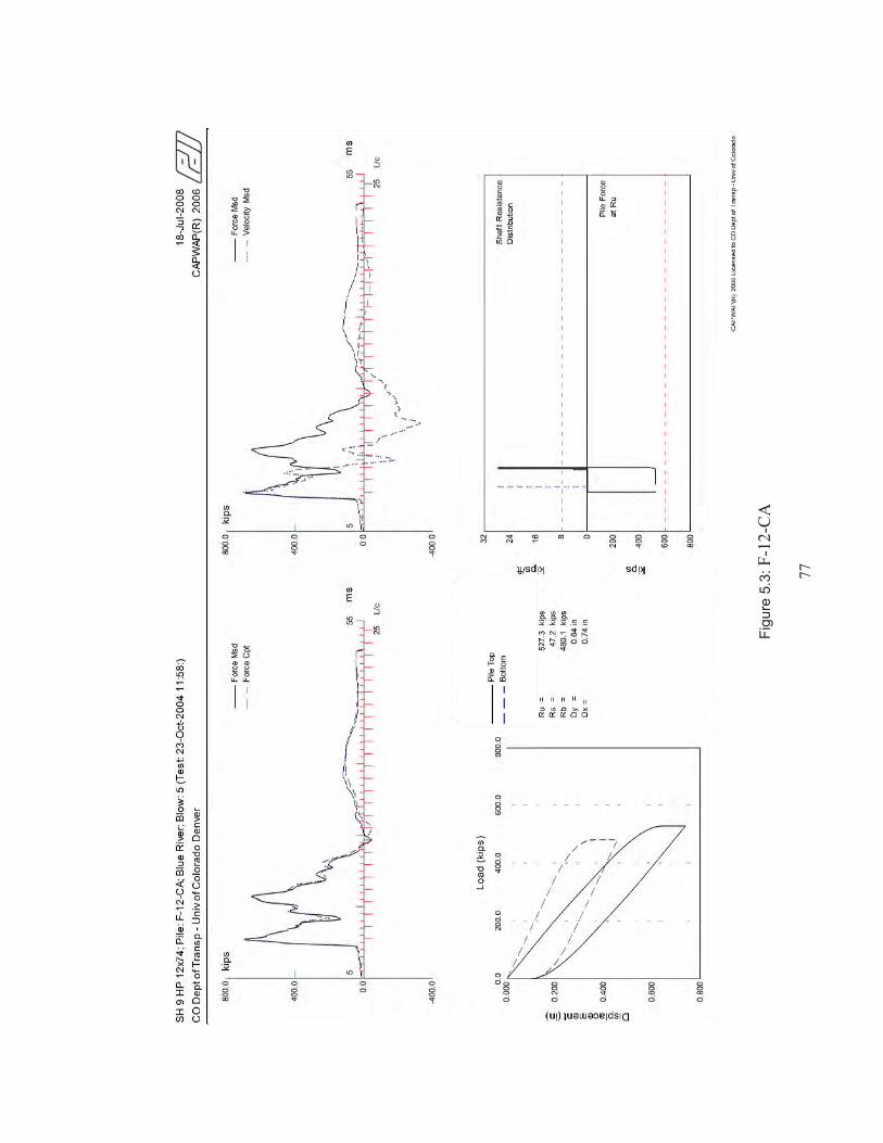
77
Figu
re 5
.3: F
-12-
CA

78
Figu
re 5
.4: D
-11-
A-1

79
Figu
re 5
.5: D
-11-
A-2
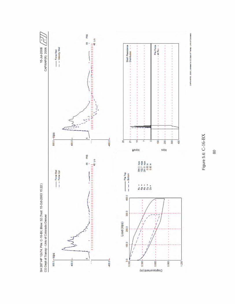
80
Figu
re 5
.6: C
-16-
BX

81
Figu
re 5
.7: C
-16-
CK
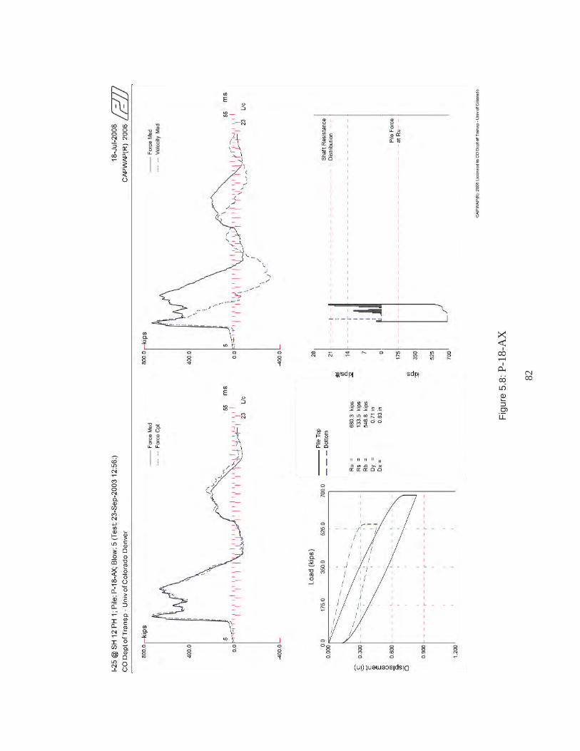
82
Figu
re 5
.8: P
-18-
AX

83
Figu
re 5
.9: L
-25-
D
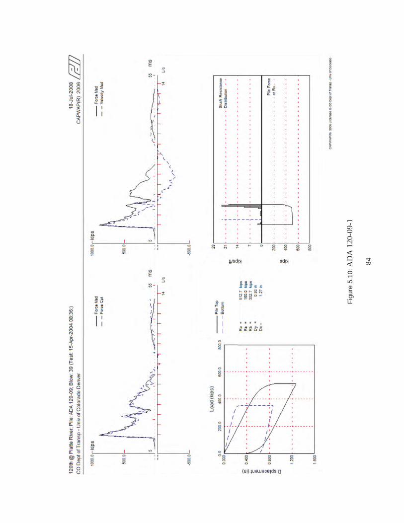
84
Figu
re 5
.10:
AD
A 1
20-0
9-1

85
Figu
re 5
.11:
AD
A 1
20-0
9-2R

86
Figu
re 5
.12:
AD
A 1
20-0
8.8W
-306
-1

87
Figu
re 5
.13:
AD
A 1
20-0
7.9E
-305

88
Figu
re 5
.14:
AD
A 1
20-0
8.8W
-306

89
Figu
re 5
.15:
CO
MC
-12-
0.2-
01A

90
Figu
re 5
.16:
H-1
7-C
J-2

91
Figu
re 5
.17:
H-1
7-C
J-1

92
Figu
re 5
.18:
D-2
0-K
-1

93
Figu
re 5
.19:
D-2
0-K

94
Figu
re 5
.20:
D-2
0-K
-5

95
Figu
re 5
.21:
D-2
0-K
-2

96
Figu
re 5
.22:
D-2
0-K
-4

97
Figu
re 5
.23:
K-1
8-G
Q

98
Figu
re 5
.24:
K-1
8-FB

99
6.0 H-PILE LENGTH IN FRONT RANGE ROCKS
6.1 Design Charts for Estimation of H-pile Length
Estimates of side resistance and end-bearing resistance in clay shale and shale derived from
DRIVEN for 12 inch H-piles are summarized in the following charts (Figures 6.1 and 6.2).
Empirical capacity estimates were derived for a box area-box perimeter resistance model
using an adhesion coefficient of 0.5 and a driving strength loss of 50 percent. Capacity
estimates are for end of drive conditions and are necessarily smaller than actual capacity with
setup time. Neglecting the contribution from overburden soil, pile length derived from these
charts will be increasingly conservative for sites with thick overburden soils. These charts are
based on rock with high RQD, greater than 70.
Energy-corrected SPT blow counts are on an equivalent foot basis for partial penetration,
with a maximum count of 200. The type of hammer used in SPT testing, manual or
automatic, must be known in order to apply the energy correction. Automatic hammers
generate high energy transfer ratios (ER) typically about 90% compared to an energy transfer
ratio of 60% for manual hammers, yielding an energy correction of 1.5 (Youd et al., 2008).
Thus, the SPT blow count for the automatic hammer is multiplied by 1.5 to correspond to
SPT blow count of a manual hammer.
6.2 Pile Length and Pile Capacity in Front Range Rocks
H 12x74 is the most frequent pile size used for bridge abutments followed by H 12x84 and H
14x89. Based on AASHTO specifications for piles with PDA monitors, an H 12x74 Grade
50 steel H-pile will have a structural capacity 360 ksi [(0.33 Fy (cross- sectional area) ],
where cross-sectional area is 21.8 in2 . To fully utilize the structural capacity, the
corresponding nominal geotechnical capacity must be greater than 514 ksi ( = 360 ksi/0.7,
resistance factor). Similarly, the nominal geotechnical capacity for H12x84 and H14x89 with
the cross-sectional areas of 24.6 and 26.1 in2, respectively, must be no less than 580 and 614
ksi, respectively. For Grade 36 H 12x74, H 12x84 and H 14x89 steel piles, to capitalize the
full structural capacities, the minimum nominal geotechnical capacities must be 373, 422 and
447, respectively. Using the design charts for side and end-bearing resistance (Figure 6.1 and
6.2), the penetration length to develop the maximum nominal resistance (end of drive) for
Grade 36 and Grade 50 steel H 12x74 piles in clay shale, shale for a range of energy
corrected uniform SPT blow count is presented in Figure 6.3. These penetration lengths are
somewhat longer than those using nominal capacity with different setup time.

Conside
load per
Table 6
shale to
gives th
overbur
GRLW
combus
than for
% of m
Figure 6
er a bridge a
r pile, numb
6.1. The pile
o very hard P
he penetratio
rden soil wa
EAP for a D
stion pressu
r Grade 36 p
aximum all
6.1 Design
abutment w
ber of piles
es are driven
Pierre Shale
on length re
as included.
Delmag D 3
ure (Table 6
pile. Drivin
lowable for
chart for SP
with a factor
and nomina
n in a geolo
e with the p
equired to d
. Piles drivin
30-32 hamm
.2). Penetra
ng stress was
Grade 50.
PT blow cou
100
ed design lo
al resistance
gic profile o
profile from
develop nom
ng stress an
mer with 80
ation length
s 71% of m
unt and side
oad of 3200
e for resista
of overburd
El Paso Co
minal resista
nd driving re
efficiency a
for Grade 5
maximum all
e resistance
0 kips. For H
ance factor o
den soil und
ounty (Figur
ance. Resista
esistance wa
and 70% of
50 pile was
lowable for
.
H 12x 74 pi
of 0.7 are sh
derlain by cl
re 6.4). DRI
ance from
as estimated
f the rated
2.5 feet lon
Grade 36 a
les, the
hown in
lay
IVEN
d using
nger
and 54

Figure 6
Figure 6
piles wi
6.2 Design
6.3 Penetrat
ith maximu
chart for SP
tion to deve
m allowabl
PT blow cou
elop nomina
e load.
101
unt and end
al resistance
d-bearing res
e for Grade
sistance.
36 and Graade 50 H 12x
x74

102
Table 6.1 Pile load, pile number, and nominal resistance for example structure
Steel Load per
Pile
Resistance
Factor
Number of Piles Nominal Resistance
Grade 50 320 kips 0.70 10 457 kips
Grade 36 228.6 kips 0.70 14 326 kips
Table 6.2 Estimated pile lengths, driving stress, and driving resistance for example structure.
Steel Estimated
Pile Length
Nominal
Resistance
GRLWEAP
Driving Stress
GRLWEAP
Driving Resistance
Grade 50 47.5 ft 472 kips 24.5 ksi 111 blows per ft
Grade 36 45 ft 326 kips 23.0 ksi 51 blows per ft
The high driving stress for Grade 50 steel allows a pile to break through thin lenses of
cemented siltstone/sandstone occurring sporadically in clay shale profiles. For the example
bridge structure, the use of Grade 50 steel would require 20 piles of 47.5 foot length versus
28 piles of 45 foot length for Grade 36 steel.
6.3 DRIVEN Capacity from Six Different Sites
Site 1 - Steel Hollow, Pueblo County, Structure K-18-HA, Abutment #3 (Figure 6.4): The
subsurface profile consists of 12 feet of sand and clay overlying hard to very hard (SPT
50/5-50/4) Pierre Shale. A 20-foot H 12x74 pile penetrated 8 feet of shale with a PDA
nominal pile capacity of 927 kips after 0.5 hours setup. DRIVEN analysis gives the pile
capacity of 515 kips at end of drive. The factored design load for the H 12x74 pile is 316 kips
with a required nominal resistance of 451 kips.

Figure 6
feet (Sit
Site 2 –
subsurf
blow co
14x89 p
0.5-hou
The des
DRIVE
Additio
Site 3 –
Abutme
overlyin
siltstone
capacity
at 38 fe
nomina
reasona
6.4 DRIVEN
te #1, Steel
– Eagleridge
face profile
ount ranging
pile penetra
ur setup. DR
sign load fo
EN analysis
onal 4-foot r
– 120th Ave
ent #1 (Figu
ng hard clay
e and sands
y of 586 kip
eet for end o
al resistance
able addition
N analysis f
Hollow, Pu
e Blvd, El P
consists of
g from 50/7
ted 10 feet
RIVEN anal
r the H 14x
(conservati
rock penetra
e @ S. Platte
ure 6.6): Th
y shale to ve
stone. A 12x
ps after 1 ho
of drive. The
e of 542 kips
nal penetrat
for EOD pil
ueblo Count
Paso County
28-foot san
7 above the t
into shale w
lysis estimat
x89 pile is 3
ve) yields th
ation yields
e River, Ad
e subsurfac
ery hard cla
x84 pile pen
our setup. D
e design loa
s. The rock
tion.
103
le capacity
ty, Structure
y, Structure
nd overlying
tip to 50/3 t
with a PDA
ted BOR ca
54 kips with
he required
430 kips.
dams County
ce profile co
ay shale wit
netrated 8.5
DRIVEN ana
ad for the H
at this site i
of a 20-foo
e K-18-HA
K-18-FB, A
g hard to ext
to 50/1 at gr
nominal ca
apacity of 4
h a required
d nominal pi
y, Structure
onsists of 38
th blow coun
feet into cl
alysis estim
H 12x84 pile
is capable o
t pile with t
, Abutment
Abutment #
tremely har
reater depth
apacity of 52
33 kips at 3
d capacity o
ile capacity
e ADA 120-
8 feet of san
nt of 50/3 w
lay shale wi
mated pile ca
e was 380 ki
of supportin
top of shale
t #3)
1 (Figure 6
rd Pierre Sh
hs. A38-foot
21 kips afte
38 feet pene
of 505 kips.
of 614 kips
-07.E305,
nd and clay
with some le
ith a PDA n
apacity of 4
ips with a re
ng this load
at 12
.5): The
ale with
t H
er
etration.
s.
enses of
nominal
476 kips
equired
at

Figure 6
is 28 fe
Figure 6
shale is
120-07.
6.5 DRIVEN
et (Site #2,
6.6 DRIVEN
38 feet (Sit
.E305, Abut
N analysis o
Eagleridge
N analysis o
te #3, 120th
tment #1)
of pile capa
Blvd, El Pa
of pile capa
Ave @ S. P
104
acity for a 4
aso County,
acity for a 4
Platte River
5 foot profi
, Structure K
6.5 foot pile
r, Adams Co
ile at end of
K-18-FB, A
e at end of d
ounty, Struc
f drive; top o
Abutment #1
drive; top o
cture ADA
of shale
1)
f clay

105
Site 4 – US 287/Berthoud Bypass, Weld County, Structure C-16-CF, Abutment #1 (Figure
6.7): The subsurface profile consists of 50 feet of soft and stiff clay overlying hard (SPT
50/12) to very hard (SPT 50/6) clay shale. An H12x74 pile penetrated 9 feet into clay shale
with a PDA nominal pile capacity of 576 kips after 6.5 hours setup. DRIVEN analysis
estimated pile capacity of 429 kips at 59 feet for end of drive. The design load was 350 kips
(close to the section limit of 360 kips) with a required nominal capacity of 500 kips.
Increasing the design load would require a 12x84 section with a maximum required
resistance of 580 kips. A longer setup time would likely achieve the required resistance as the
section is all moist clay and clay shale and strength gain with longer setup time is likely.
Site 5 – I-25@SH7, Weld County, Structure D-17-CT, Abutment #1 (Figure 6.8): The
subsurface profile consists of 18 feet of stiff clay overlying hard (SPT 50/12, 50/10, 50/7)
clay shale that did not show consistent strength increase with depth. Adjacent deeper boring
does not show SPT higher than 50/10 for a 10 foot interval past the pile tip. An H 12x74 pile
penetrated 13.6 feet of clay shale with a PDA nominal pile capacity of 466 kips after 1 hour
setup. DRIVEN analysis estimated pile capacity of 359 kips at 31.6 feet for end of drive. The
design load was 326 kips with a required resistance of 466 kips. DRIVEN estimates a 500 kip
nominal pile capacity with additional 10 foot penetration into rock.
Site 6 – SH 9/E of Kremmling, Grand County, Structure D-11-A, Abutment #1 (Figure 6.9):
The subsurface profile consists of 48 feet of clayey sand and gravelly sand overlying medium
hard and hard clay shale (SPT 40/12-77/12) that shows a gradual strength increase with
depth. An H 12x74 pile penetrated 20 feet of clay shale with PDA nominal pile capacity of
672 kips after 1.5 hours setup. DRIVEN analysis below estimated pile capacity of 520 kips at
68 feet for end of drive. The factored design load for was 285 kips with a required resistance
of 408 kips.

Figure 6
shale is
Figure 6
shale is
6.7 DRIVEN
50 feet (Sit
6.8 DRIVEN
18 feet (Sit
N analysis o
te #4, abutm
N analysis o
te #5, I-25@
of pile capa
ment #1, stru
of pile capa
@SH7, Wel
106
acity for a 5
ucture C-16
acity for a 4
d County, S
9 foot pile a
6-CF with te
2 foot profi
Structure D-
at end of dr
est pile)
ile at end of
-17-CT, Ab
ive; top of c
f drive; top o
butment #1)
clay
of clay

Figu
shale i
6.4 Pile
It was m
approxi
into Pie
shale be
blow co
A plot o
resistan
foot of p
the bori
penetrat
because
resistan
when th
the adva
440 kip
kips (Ra
pile cap
ure 6.9 DRIV
s 48 feet (S
e Resistanc
most benefic
imately 1-fo
erre Shale F
eing weathe
ount of 50/5
of PDA nom
nce after abo
penetration
ing log prof
ting into cla
e of the poss
nce of soil-p
he pile is str
ancement o
ps at restrike
ausche, 198
pacity of 40
VEN analys
ite #6, SH 9
e and Pene
cial that, in
oot intervals
ormation at
ered, the blo
5. Static load
minal capac
out 3 to 4 fe
(Figure 6.1
file (Figure
ay shale typ
sibility of fo
pile interface
ruck. With e
of pile tip. T
e with shaft
89). A static
0 kips. Othe
sis of pile ca
9/E of Krem
etration Len
1988, CDO
s and follow
t SH 24 nea
ow count inc
d tests were
ity versus p
eet of penetr
10). Pile, ha
6.11). As d
pically expe
ormation of
e friction an
each hamme
The PDA rec
side resista
c load test u
er three pile
107
apacity for a
mmling, Gra
#1)
ngth
OT conducte
wed up with
ar Colorado
creases rapi
e conducted
pile penetrat
ration to the
ammer and m
discussed ea
rience signi
f plugged co
nd adhesion
er blow, an
cord from te
ance of 137
using Daviss
e data will b
a 68 foot pi
and County,
ed a series o
h static load
Springs. Be
idly to very
d after the pe
tion length s
e resistance
measuremen
arlier, the en
ificant end b
ondition at t
n along the p
interface sh
est pile #2 in
kips and en
son failure c
be analyzed
ile at end of
, Structure D
of PDA mea
tests on fou
esides the u
y hard clay s
enetration to
shows a rap
increase of
nt informati
nd bearing c
bearing cap
the end of p
pile-web int
hear failure
ndicates a n
nd-bearing r
criteria mea
during Pha
f drive; top o
D-11-A, Ab
asurements
ur H-piles d
upper 1 foot
shale with fi
o a design d
pid increase
f about 100
ion are show
capacity of H
pacity increa
piles. The co
terface is ac
took place
nominal cap
resistance o
asured an ult
ase II of this
of clay
butment
at
driven
of clay
field
depth.
of pile
kips per
wn on
H-piles
ase
ombined
ctivated
during
pacity of
f 303
timate
s study.

Figure 66.10 Pile caapacity withh increasing
108
penetrationn length intoo clay shalee.

Figgure 6.11 Booring log pr
109
rofile of secttion at SH 224 pile test site.

110
7.0 SUMMARY, CONCLUSIONS, AND FURTHER STUDY
7.1 Summary The final report on “CDOT Foundation Design Practice and LRFD Strategic Plan” was submitted in 2006, which addresses the need to continue the research on the evaluation of Colorado-specific geotechnical resistance a factors. This report on “CDOT Strategic Plan for Data Collection and Evaluation of Grade 50 H-Piles into Bedrock” addresses the issues toward the eventual evaluation of the Colorado-specific resistance factors for driven pile designs. The report has gone much beyond the original plan for Phase I research and presents some results for Phase II research. Some research findings are recommended for implementation in CDOT driven pile design practices. This report summarizes the effort toward the evaluation of the benefits derived from the shifting to Grade 50 from Grade 36 in the production of steel H- and pipe piles. With a higher yield strength of Grade 50 steel than Grade 36, piles can be driven deeper to stronger rocks with a larger hammer to reduce driving resistance in terms of blow counts per foot of pile tip penetration with a proper pile over stressing risk management. This necessarily leads to a higher pile capacity and reduced number of piles required in support a bridge load in a pile group, and therefore project cost savings. This report summarizes the findings from the Phase I research.
The Phase II study is planned to focus on the evaluation of resistance factors with a limited statistical sample size. The sample size could be increased with CDOT performing static load tests and the availability of test data for driven piles. All test additional driven piles with PDA measurements will be analyzed. Upon completion of Phase II the geotechnical engineers in Colorado should be able to perform the LRFD design of driven piles with increasing confidence. Because of a small Colorado statistical sample size for driven pile static load tests, a proposal, in addition to the Phase II study proposal, might be submitted to Colorado’s neighboring states for a pooled-fund study to take advantage of their existing static load test data base with piles installed in rocks similar to Colorado rocks. This joint effort should result in the resistance factors applicable to the driven pile design in all contributors to this project.
7.2 Findings of this Study The findings from this Phase I study are outlined as follows: 1. Grade 50 steel piles can be driven deeper to achieve higher capacities because of the
higher allowable dynamic driving stress of Grade 50 steel and, thereby, a smaller number of piles are needed to support a bridge load.
2. For twenty four piles analyzed as shown in Table 2.1, the capacity from CASE method is 28 percent higher than the CAPWAP prediction via signal matching and DRIVEN 10

111
percent higher than the CAPWAP calculation. This means that CASE can over-predict the pile capacity and CAPWAP is strongly urged for checking the capacity.
3. Piles driven into the Colorado rock formations are of moderate lengths and most of the driving stresses are lower than 45 ksi, allowable driving stress. Thus, piles can be driven deeper to derive higher capacity without over stressing.
4. This study should be extended to cover steel H-piles ranging 16 to 24 inches to examine the gives and takes of these piles with sizes larger than 12 and 14 inch piles currently adopted in the driven pile design. When found feasible with higher nominal capacities, a fewer piles might be needed and further construction cost saving might be realized because of a fewer piles needed.
5. When using DRIVEN for H-pile capacity calculation for clay shale, options are available to use the box or flange perimeter for calculating the side shear resistance, and the box area at the pile tip for end bearing.
6. For H-piles in uncemented and partially cemented sandstone, the total pile box perimeter times pile length is recommended for computing side shear resistance and the pile box area is recommended to computing the end bearing capacity.
7. For H-piles and pipe piles driven into weak rocks, sand, gravel and/or clay, it is recommended, when using GRLWEAP, to use 80 percent hammer efficiency and 70 to 90 percent of rated combustion pressure.
8. PDA at re-strike yields a higher pile capacity than the end of drive (EOD) capacity. The amount of capacity gain depends on waiting period termed “setup time” and soil and rock types. Saturated clayey soil and clay shale are expected to derive higher capacity gain during the setup time, while rate of capacity decreases significantly with time.
9. Driving resistances are more variable than driving stresses in GRLWEAP analyses and usually the analysis will results in higher driving resistance with reasons yet to be explored and yet piles were driven successfully with much smaller driving resistance. So it is recommended not to reject the hammer or driving plan solely on driving resistance estimated in GRLWEAP analysis, instead, exercise good engineering judgment in making decisions.
7.3 Recommendations for Further Research A separate proposal will be submitted for the Phase II study, but it will include the following study items and beyond:
1. The full benefits of using Grade 50 steel piles is the enhancement of the pile capacity because of the higher permissible driving yield stress of 45 ksi. With increased capacity, much cost saving will be realized.

112
2. Analyze the PDA pile driving data for evaluating the nominal pile capacity using CASE method. CAPWAP signal matching, GRLWEAP, and DRIVEN , etc. will be performed on all available test piles for the evaluation of geotechnical resistance factors.
3. To capitalize on the capacity increase with setup time, it is strongly recommended to perform a few PDA monitored pile driving at difference setup time. This will help assess the capacity gain of driven piles in Colorado geological conditions.
4. It is strongly recommended to perform additional static load tests to provide a database for the calibration of resistance factor for Colorado driven pile design.
5. To investigate the effect of steel H-pile size on pile capacities beyond 12-inch steel H-piles. A larger pile with higher capacity might further reduce pile-installation cost.
6. With the small number of load tested H-piles in CDOT’s collection, the procedures for the database with small statistical sample size will be adopted in evaluating the resistance factor for driven pile design in Colorado.
7. All available feasible tools for the analysis and design of driven piles in Colorado will be used in the Phase II study to identify the one(s) most fit for CDOT and the Colorado geotechnical industry.
8. A pooled-fund study with neighboring states of similar geological conditions will be recommended to pool the static load test data from each participating state with the intent of enhancing the data base and associated resistance factors for driven pile designs appropriate for all participating states.

113
REFERENCES
AASHTO. (2007). Standard specifications for highway bridge, 4th edition. American Association of State Highway and Transportation Officials, Washington, D.C.
AASHTO. (2010). Standard specifications for highway bridges, 5th edition. American Association of State Highway and Transportation Officials, Washington, D.C.
Abu-Hejleh, N., O’Neill, M.W., Hannerman, D., & Attwooll, W.J. (2003). Improvement of the geotechnical axial design methodology for Colorado’s drilled shafts socketed in weak rocks: report CDOT-DTD-R-2003-6. Colorado Department of Transportation, Denver, Colorado.
Azizi, F. (2000). Applied Analysis in Geotechnics, 1st edition. E & FN Spon, London.
Bond, A.J., & Jardine, R.J. (1991). Effects of installing displacement piles in a high OCR clay. Geotechnique, 4(3), 341-363.
Botts, M.E. (1986). The effects of slaking on the engineering behavior of clay shales (Unpublished doctoral dissertation). University of Colorado, Boulder, Colorado.
CAGE, (1999). Drilled pier design criteria for lightly loaded structures in the Denver metropolitan area. Colorado Association of Geotechnical Engineers, Denver, Colorado.
Cesare, J.A., Duran, D.R., Lewis, N.F., & Limbach, F.W. (2002). Results and design recommendations from geotechnical investigations on the Northwest Parkway and E- 470. ASCE Symposium, Denver, Colorado.
Chen, F.H. (1999). Soil engineering: testing, design and remediation. CRC Press, Boca Raton, Florida.
Chow, F.C., Jardine, R.J., Nauroy, J.F. & Brucy, F. (1997). Time-related increase in shaft capacities of driven piles in sand. Geotechnique, 47(2), 353-361.
Goble, G.G., & Rausche, F. (1976). Wave equation analyses of pile driving-program manuals:report No. FHWA IP-76-14.3. Department of Transportation, Federal Highway Administration, Washington, D.C.

114
Coduto, D.P. (2001). Foundation design principles and practices, 2nd edition. Prentice-Hall, Upper Saddle River, New Jersey.
Fellinius, B.H., Riker, R.E., O’Brien, A.J., & Tracy, G.R. (1989). Dynamic and static testing in a soil exhibiting set-up. American Society of Civil Engineers, Journal of Geotechnical Engineering Division, 115 (7), 984-1001.
Goodman, R.E. (1993). Engineering geology-rock in engineering construction, 1st edition. John Wiley & Sons, New York.
GRL, (2005). GRLWEAP-wave equation analysis of pile driving manual. GRL, Cleveland, Ohio.
Hannigan, P.J. Goble, G.G., Thendean, G., Likins, G.E., & Rausche, F. (1998). Design and construction of driven pile foundations: report FHWA-HI-97-013. Department of Transportation, Federal Highway Administration, Washington, D.C.
Likins, G. E. (2010). The 2010 AASHTO LRFD resistance factors. Pile Driver Magazine, 2, 43-51.
Mathias, D. & Cribbs, M. (1998). Driven 1.0: program for determining ultimate vertical static pile capacity: report FHWA-SA-98-074. Department of Transportation, Federal Highway Administration, Washington, D.C.
Mead, W.J. (1936). Engineering geology of damsites. Transactions 2nd International Congress on Large Dams, Paris, France, p. 171-192.
Meyerhof, G.G. (1976). Bearing capacity and settlement of pile foundations. American Society of Civil Engineers, Journal of Geotechnical Engineering Division, 102, GT3, 195-228.
Nordland, R.L. (1963). Bearing capacity of piles in cohesionless soils. American Society of Civil Engineers, Soil Mechanics & Foundations Journal, 89(SM-3).
Nordland, R.L. (1979). Point bearing and shaft friction of piles in sand. 5th Annual Short Course on the Fundamentals of Deep Foundation Design, Missouri-Rolla.

115
O’Neill, M.W. (1983). Group action in offshore piles. In S.G. Wright Editor, Proceedings of the Conference on Geotechnical Practice in Offshore Engineering, American Society of Civil Engineers, New York.
O’Neill, M.W., Townsend, F.C., Hassan, K.M., Buller, A., & Chan, P.S. (1996). Load transfer for drilled shafts in intermediate geomaterials: report FHWA-RD-95-72. U.S. Department of Transportation, Federal Highway Administration, Washington, D.C.
O’Neill, M.W., & Reese, L.C. (1999). Drilled shafts construction procedures and design methods: report FHWA-IF-99-025. U.S. Department of Transportation, Federal Highway Administration, Washington, D.C.
Peterson, R. (1958). Rebound in the Bearpaw Shale, Western Canada. Geological Society of America Bulletin, 69(3), 171-192.
Rausche, F., Goble, G. G., & Likins, G. E. (1985). Dynamic determination of pile capacity. American Society of Civil Engineers, Journal of the Geotechnical Engineering Division, 111(3), 367-383.
Rausche, F., Goble, G. G., & Likins, G. E. (1992). Investigation of dynamic soil resistance on piles using GRLWEAP. Proceedings of the Fourth International Conference on the Application of Stress-Wave Theory to Piles, The Netherlands, p.137-142.
Rausche, F., Thendean, G., Abou-Matar, H., Likins, G., & Goble, G. (1996). Determination of pile drivability and capacity from penetration tests: FHWA contract No. DTFH61-91-C-00047, final report. U.S. Department of Transportation, Federal Highway Administration, Washington, D.C.
Seed, H.B., & Reese, L.C. (1955). The action of soft clay along friction piles. Transactions American Society of Civil Engineers, 122, 731-754.
Semple, R.M., & Rigden, W.J. (1984). Shaft capacity of driven pipe piles in clay. In J.R. Meyer Editor, Analysis and Design of Pile Foundations. American Society of Civil Engineers, New York.
Smith, E.A.L. (1960). Pile driving analysis by the wave equation. American Society of Civil Engineers, Journal of Soil Mechanics and Foundations, 86, SM4, 35-61.

116
Terzaghi, K., Peck, R.B., & Gholomrera, M. (1996). Soil mechanics in engineering practice, 3rd
edition. John Wiley & Sons, New York.
Thompson, C.D., & Thompson, D.E. (1985). Real and apparent relaxation of driven piles.
American Society of Civil Engineers, Journal of Geotechnical Engineering Division, 111(2),
225-237.
Tomlinson, M.J. (1980). Foundation design and construction, 4th edition. Pitman, London.
Tomlinson, M.J. (1994). Pile design and construction practices, 4th edition. E & FN Spon, London.
Topper, R., Spray K.L., Bellis, W.H., Hamilton, J.L., & Barkmann, P.E. (2003). Ground Water
Atlas of Colorado. Colorado Geological Survey, Denver, Colorado.
Trimble, D.E. (1980). Geologic story of the great plains. U.S. Geological Survey Bulletin 1493,
Washington, D.C.
Wyllie, D.C. (1999). Foundations on rock, 2nd edition. E & FN Spon, London.
Youd, T.L., Bartholomew, H.W., & Steidl, J. H. (2008). SPT hammer energy ratio versus drop
height. American Society of Civil Engineers, Journal of Geotechnical and Geoenvironmental
Engineering, 134(3), 397-400.

A-1
APPENDIX A – BORING LOG PROFILES

A-2

A-3
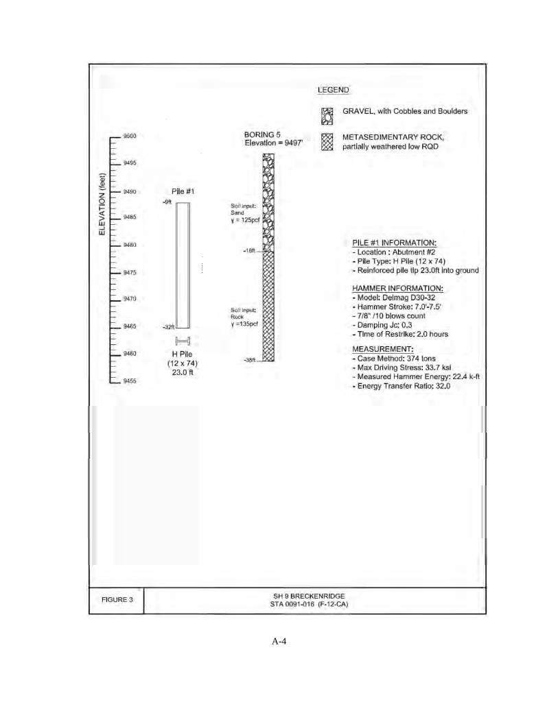
A-4

A-5

A-6

A-7

A-8

A-9

A-10

A-11

A-12

A-13

A-14

A-15

A-16

A-17

A-18

A-19

A-20

A-21

A-22
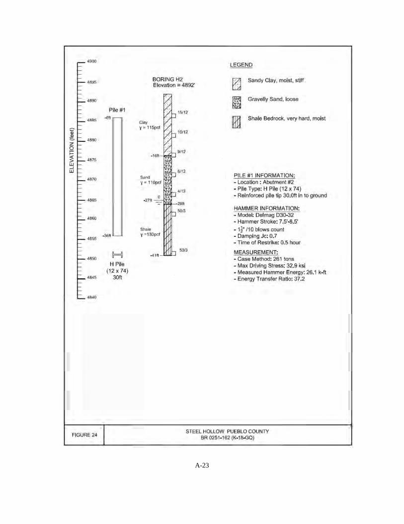
A-23