Causes and Consequences of the Oil Shock of 2007-08*

James D. Hamilton

jhamilton@ucsd.edu

Department of Economics, UC San Diego

February 3, 2009 Revised: April 27, 2009

ABSTRACT

This paper explores similarities and differences between the run-up of oil prices in 2007-

08 and earlier oil price shocks, looking at what caused the price increase and what effects it

had on the economy. Whereas historical oil price shocks were primarily caused by physical

disruptions of supply, the price run-up of 2007-08 was caused by strong demand confronting

stagnating world production. Although the causes were different, the consequences for

the economy appear to have been very similar to those observed in earlier episodes, with

significant effects on overall consumption spending and purchases of domestic automobiles in

particular. In the absence of those declines, it is unlikely that we would have characterized

the period 2007:Q4 to 2008:Q3 as one of economic recession for the U.S. The experience

of 2007-08 should thus be added to the list of recessions to which oil prices appear to have

made a material contribution.

∗I am grateful to Alan Blinder, David Romer, Lutz Kilian, conference participants, and

an anonymous referee for helpful comments on an earlier draft of this paper, and to Davide

Bertoli for supplying the Blanchard-Galí data and code.

1 Introduction.

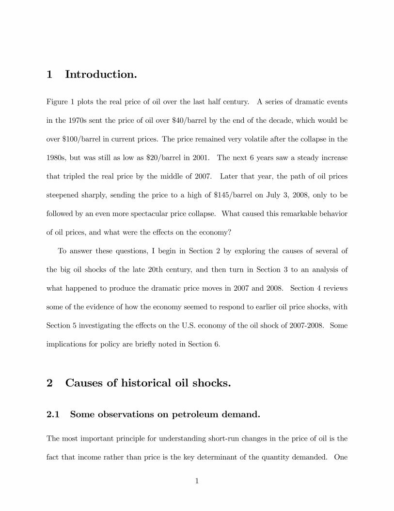
Figure 1 plots the real price of oil over the last half century. A series of dramatic events

in the 1970s sent the price of oil over $40/barrel by the end of the decade, which would be

over $100/barrel in current prices. The price remained very volatile after the collapse in the

1980s, but was still as low as $20/barrel in 2001. The next 6 years saw a steady increase

that tripled the real price by the middle of 2007. Later that year, the path of oil prices

steepened sharply, sending the price to a high of $145/barrel on July 3, 2008, only to be

followed by an even more spectacular price collapse. What caused this remarkable behavior

of oil prices, and what were the effects on the economy?

To answer these questions, I begin in Section 2 by exploring the causes of several of

the big oil shocks of the late 20th century, and then turn in Section 3 to an analysis of

what happened to produce the dramatic price moves in 2007 and 2008. Section 4 reviews

some of the evidence of how the economy seemed to respond to earlier oil price shocks, with

Section 5 investigating the effects on the U.S. economy of the oil shock of 2007-2008. Some

implications for policy are briefly noted in Section 6.

2 Causes of historical oil shocks.

2.1 Some observations on petroleum demand.

The most important principle for understanding short-run changes in the price of oil is the

fact that income rather than price is the key determinant of the quantity demanded. One

1

quick way to become convinced of this fact is to examine Figure 2, which plots petroleum

consumption against GDP for the U.S. over the last 60 years.1 Despite the huge fluctuations

in the relative price of oil over this period, petroleum consumption followed income growth

remarkably steadily. There was some downward adjustment in oil use at the end of the

1970s, though achieving that 20% drop in petroleum consumption required an 80% increase

in the relative price and two recessions in a 3-year period over 1980-82.

There is a flattening in the slope of this path over time, which some might attribute

to delayed conservation consequences of the 1970s oil shocks. However, this flatter slope

persists long after the price had fallen quite dramatically, and seems more likely to be due

to the fact that income elasticity declines as a country becomes more developed. One sees

a similar pattern of slowing growth of petroleum use as other developed countries became

richer, while post-1990 data for the newly industrialized countries is still quite supportive of

an income elasticity near unity (Hamilton, 2009; Gately and Huntington, 2002).

Table 1 summarizes the estimated price elasticities for gasoline and crude oil demand

from a half-dozen meta-analyses or literature reviews. Since crude oil represents about half

the retail cost of gasoline, one would expect that a 10% increase in the price of crude would

be associated with a 5% increase in the price of gasoline,2 in which case the price elasticity

of the demand for crude oil should be about half as big as that for retail gasoline. Most of

1 This is essentially a scatterplot with adjacent years connected by a smoothed curve. Tracing this curvefrom the lower left to the upper right identifies the combinations of real GDP and petroleum consumptionthat were observed at increasingly later dates as one moves along the curve.

2 The regression coefficient relating the log of the nominal U.S. gasoline retail price to the logof the nominal WTI in a monthly cointegrating regression estimated over 1993:M4-2008:M8 is 0.62.Data from EIA, “Spot Prices for Crude Oil and Petroleum Products,” http://tonto.eia.doe.gov/dnav/pet/pet_pri_spt_s1_m.htm.

2

the studies behind these summaries reported low estimates of the price-elasticity of gasoline

demand and significantly smaller elasticities for crude.

The price elasticity of petroleum demand has always been small, and it is hard to avoid

any conclusion other than that it had become an even smaller number for the U.S. in the

2000s. One can barely detect any downward deviation from the trend in petroleum con-

sumption in Figure 2 despite the enormous price increase through 2007. Hughes, Knittel,

and Sperling (2008) estimated that short-run gasoline demand elasticity was in the range of

0.21 to 0.34 over 1975-1980 but between only 0.034 and 0.077 for the 2001-06 period.

Another key parameter for determining the consequences of an energy price increase for

the economy is the value share of energy purchases relative to total expenditures. The

fact that the U.S. income elasticity of demand has been substantially below unity over the

last quarter century induces a downward trend in that share— for a given relative price, if

the percentage growth in energy use is less than the percentage growth in income, total

dollar expenditures on energy would decline as a percentage of income. On the other hand,

the very low short-run price elasticity of demand causes the value share to move in the

same direction as the relative price— if the percentage increase in price is greater than the

percentage decrease in quantity demanded, dollar spending as a share of income will rise

when the price of energy goes up.

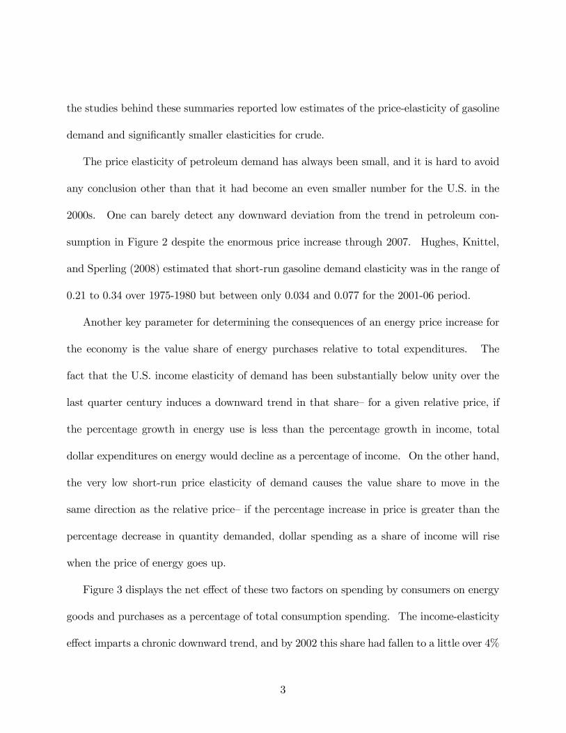
Figure 3 displays the net effect of these two factors on spending by consumers on energy

goods and purchases as a percentage of total consumption spending. The income-elasticity

effect imparts a chronic downward trend, and by 2002 this share had fallen to a little over 4%

3

of a typical consumer’s total budget. However, subsequent energy price increases produced

a dramatic reversal of this trend, with the share in 2008 almost twice the 2002 value.

Figure 3 also serves to remind us that a price elasticity cannot be globally below unity.

If you don’t reduce the quantity purchased by as much in percentage terms as the price

goes up, the item comes to consume a larger fraction of your budget. If the price elasticity

were globally less than unity, an arbitrarily large price increase would ultimately bring the

consumer to a point where 100% of the budget was going to energy, in which case ignoring

the price would no longer be physically possible. The low expenditure share in the early

part of this decade may be part of the explanation for why Americans were largely ignoring

the early price increases— we didn’t change our behavior much because most of us could

afford not to. By 2007-08, however, the situation had changed, as energy had once again

returned to an importance for a typical budget that we had not seen since the 1970s.

2.2 Historical supply disruptions.

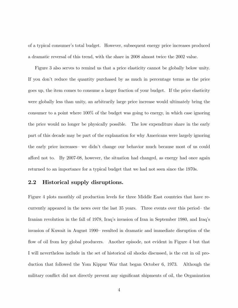
Figure 4 plots monthly oil production levels for three Middle East countries that have re-

currently appeared in the news over the last 35 years. Three events over this period— the

Iranian revolution in the fall of 1978, Iraq’s invasion of Iran in September 1980, and Iraq’s

invasion of Kuwait in August 1990— resulted in dramatic and immediate disruption of the

flow of oil from key global producers. Another episode, not evident in Figure 4 but that

I will nevertheless include in the set of historical oil shocks discussed, is the cut in oil pro-

duction that followed the Yom Kippur War that began October 6, 1973. Although the

military conflict did not directly prevent any significant shipments of oil, the Organization

4

of Arab Petroleum Exporting Countries (OAPEC) announced3 on October 16 that it would

cut production by 5%

until the Israeli forces are completely evacuated from all the Arab territories

occupied in the June 1967 war and the legitimate rights of the Palestinian people

are restored.

Hamilton (2003) included the Suez Crisis of 1956 as a fifth significant oil shock, though

the price increase from that episode was much more modest, and data for the kinds of

comparisons performed below are not readily available for that period, so this paper will use

just these four episodes.

The bold line in the first column of Figure 5 records the drop in oil production from the

affected countries in the months following the events just mentioned. The first panel in

that column uses the combined output of the members of OAPEC. The panel in the second

row, first column shows the production from Iran. The third row of column 1 gives the

combined production of Iran and Iraq, and the fourth row the combined production of Iraq

and Kuwait. In each case, the production shortfall is expressed as a percentage of total

global production prior to the shock.4 Each of these events knocked out between 7 and 9

percent of world supply.

3 Quotation is taken from an OAPEC ministers’ press release reported by Al-Sowayegh (1984, p. 129).

4 These numbers differ slightly from the values reported in Table 4 of Hamilton (2003) due to smalldifferences in the estimates of total global oil production used, and the fact that here the Iranian shortfallis dated as beginning in October rather than September of 1978.

5

In each episode, there was some increase in production coming from other countries that

partially mitigated the consequences. The net consequences of the disruptions are captured

by the dashed lines in the first column of Figure 5, which portray the percentage decline in

actual total world production following each of the events. Production increases from other

countries were rather minor in 1973-74, but quite substantial in 1990-91.

The subsequent path of oil prices is indicated in the second column of Figure 5. Each

of these episodes was associated with significant increases in the price of oil, with the price

jumping 25% in 1980 and 70% in 1990. Note that there were some price controls in effect

for the first three episodes, which spread the consequences over time.

Kilian (forthcoming) downplays the contribution of these supply disruptions to the price

movements portrayed in Figure 5, instead attributing much of the historical fluctuations in

the price of oil to what he describes as “precautionary demand associated with market con-

cerns about the availability of future oil supplies.” He identifies the latter as any movements

in the real price of oil that cannot be explained statistically by his measures of shocks to

supply and aggregate demand. Another way one might try to measure the contribution of

precautionary demand is by looking at changes in inventories. The third column of Figure

5 records the monthly change in U.S. inventories of crude oil and petroleum products be-

ginning with the first month of each of the four episodes, again measured as a percentage of

total global production. In each of these episodes, inventories were going down, not up, at

the time of the sharpest price movements, suggesting that inventory changes were serving

to mitigate rather than aggravate the magnitude of the price shocks. Positive inventory

6

investment typically came much later, as firms sought to restock the storage that had been

earlier drawn down.

One can also explore whether the supply disruptions alone offer a sufficient explanation

for the observed price movements on the basis of plausible elasticities. Table 2 compares the

average decline in global oil production during these four episodes with the observed price

change to calculate implied price-elasticities of demand under the assumption that there was

zero shift in demand from growing income over these episodes and that the supply shift was

the sole explanation for the price increase. These elasticities are a bit smaller than might

have been expected from the consensus estimates in Table 1, but in no case does it seem

implausible on the basis of the implied elasticity to attribute most of the price change to the

supply shortfall itself.

Kilian (2008) also argues that the bold lines in the first column of Figure 5 overstate the

magnitude of the supply disruptions caused by these 4 episodes. He observes, for example,

that Iraq increased production significantly in anticipation of both the 1980 and 1990 wars,

so that using the Iraqi production levels just prior to the conflict overstates the size of the

shock (see the middle panel of Figure 4). Note, however, that this is not a factor in the

dashed lines of Figure 5 or the calculations in Table 2, which are based on the observed global

decline subsequent to the indicated date. Moreover, despite the high levels of pre-war Iraqi

production, global production in September 1980 was 2.9% below its level 3 months earlier

and 5.4% below its level of 6 month earlier. Likewise, global production in July 1990 was

down 2.1% or 0.7% from its values 3 months or 6 months earlier. Hence, if we’d compared

7

global production in these episodes with a value earlier than the September 1980 or July

1990 reference dates used, the imputed quantity reductions in Table 2 would have been even

more significant.

Kilian (forthcoming) and Barsky and Kilian (2002) argue, quite correctly in my view,

that demand pressures also made a contribution to the magnitudes of the oil price increase

observed in several of these episodes. In particular, it would be irresponsible to claim that

the nominal oil price increase in 1973-74 had nothing to do with the general inflation and

boom in the prices of other commodities also observed at that time. Nevertheless, I share

Blinder and Rudd’s (2008) doubts about whether inflationary pressures can be construed as

the primary explanation for why OAPEC chose to reduce the quantity of oil they produced

by 5% within weeks of the onset of the Yom Kippur War.

My overall conclusion thus supports the conventional interpretation: historical oil price

shocks were primarily caused by significant disruptions in crude oil production that were

brought about by largely exogenous geopolitical events.

3 Causes of the oil shock of 2007-08.

Figure 6 plots five different measures of energy prices during the last quarter of 2007 and

first half of 2008. By any measure, this episode qualifies as one of biggest shocks to oil

prices on record. However, the causes were quite different from events associated with the

4 episodes examined above.

8

3.1 Supply.

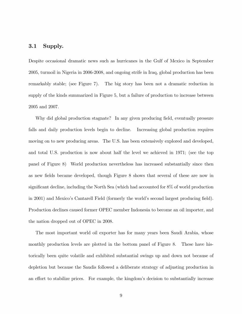
Despite occasional dramatic news such as hurricanes in the Gulf of Mexico in September

2005, turmoil in Nigeria in 2006-2008, and ongoing strife in Iraq, global production has been

remarkably stable; (see Figure 7). The big story has been not a dramatic reduction in

supply of the kinds summarized in Figure 5, but a failure of production to increase between

2005 and 2007.

Why did global production stagnate? In any given producing field, eventually pressure

falls and daily production levels begin to decline. Increasing global production requires

moving on to new producing areas. The U.S. has been extensively explored and developed,

and total U.S. production is now about half the level we achieved in 1971; (see the top

panel of Figure 8) World production nevertheless has increased substantially since then

as new fields became developed, though Figure 8 shows that several of these are now in

significant decline, including the North Sea (which had accounted for 8% of world production

in 2001) and Mexico’s Cantarell Field (formerly the world’s second largest producing field).

Production declines caused former OPEC member Indonesia to become an oil importer, and

the nation dropped out of OPEC in 2008.

The most important world oil exporter has for many years been Saudi Arabia, whose

monthly production levels are plotted in the bottom panel of Figure 8. These have his-

torically been quite volatile and exhibited substantial swings up and down not because of

depletion but because the Saudis followed a deliberate strategy of adjusting production in

an effort to stabilize prices. For example, the kingdom’s decision to substantially increase

9

production in late 1990 was a reason why the oil price shock of 1990 was so short-lived (see

the bottom row of Figure 5).

Because the Saudis had historically used their excess capacity to mitigate the effects

of short-run supply shortfalls, many analysts had assumed that they would continue to

do the same in response to the longer run pressure of growing world demand, and most

forecasts called for continuing increases in Saudi production levels over time. For example,

even as recently as in their 2007 World Energy Outlook, the International Energy Agency

was projecting that the Saudis would be pumping 12 million barrels per day by 2010. In

the event, however, Saudi production went down rather than up in 2007. It is a matter of

conjecture whether the decline in Saudi production in 2007 should be attributed to depletion

of its Ghawar oil field, to a deliberate policy decision in response to a perceived decline in

the price-elasticity of demand, or to long-run considerations discussed below. Whatever its

cause, the decline in Saudi production was certainly one important factor contributing to

the stagnation in world oil production over 2005-2007. It also unambiguously denotes the

latter episode as a new era as far as oil pricing dynamics are concerned— without the Saudis’

willingness or ability to adjust production to smooth out price changes, any disturbance to

supply or demand would have a significantly bigger effect on price after 2005 compared with

earlier periods.

3.2 Demand.

Although supply stagnated, demand was growing strongly. Particularly noteworthy is oil

consumption in China, which has been growing at a 7% compound annual rate over the

10

last two decades; (see Figure 9). Chinese consumption in 2007 was 870,000 barrels per day

higher in 2007 than it had been in 2005.

How can it be that China was consuming more oil, yet no more oil was being produced?

Mathematically, consumption in other regions had to decline, and indeed it did. Consump-

tion in the U.S. in 2007 was 122,000 b/d below its level in 2005; Europe dropped 346,000 and

Japan 318,000. And what persuaded residents of these countries to reduce oil consumption

in the face of rising incomes? The answer is, the price had to increase sufficiently to reduce

consumption in the OECD countries commensurate with the increase from China, given the

stagnation in total global production.

Let us consider some quick ballpark estimates of how big a price increase that should have

required. According to IMF estimates,5 World real GDP experienced 2-year total growth

of 9.4% in 2004 and 2005. As noted above, the income elasticity of petroleum demand in

countries like the U.S. is currently about 0.5, whereas in the newly industrialized countries

it may be above unity (Hamilton, 2009; Gately and Huntington, 2002). World petroleum

production was 5 million barrels per day higher in 2005 than in 2003, a 6% increase. Thus it

is entirely plausible to attribute the 6% increase in oil consumption between 2003 and 2005

to a shift in the demand curve caused by the increase in world GDP.

World real GDP grew an additional 10.1% in 2006 and 2007. Hence it seems reasonable

to suppose that, if oil had remained at the 2005 price of $55/barrel, quantity demanded

would have increased by at least another 5 million barrels per day by the end of 2007. Eco-

5 IMF, World Economic Outook: October 2008, Table A.1.

11

nomic growth slowed significantly in 2008:H1, but remained positive, and I’ve conservatively

assumed that economic growth would have added at least another half million barrels per

day to the quantity demanded in the first half of 2008, more than enough to absorb the

slight increase in global production that finally appeared in the first half of 2008. Under

these assumptions, the price had to rise between 2005 and 2008:H1 by an amount sufficient

to reduce the quantity demanded by 5 mb/d; (see the top panel of Figure 10).

It’s worth commenting on what was new about the contribution of Chinese and world

economic growth over this period. While China had been growing at the remarkable rate

noted for a quarter century, it has only recently become big enough relative to the global

economy to make a material difference. For example, the 4.9% world GDP average annual

growth rate over 2003-2007 compares with a 2.9% average over the robust 1990s. And

judging from the gap between EIA figures for China’s total petroleum production and con-

sumption,6 China was a net exporter of petroleum up until 1992, and its imports were only

up to 800,000 barrels/day in 1998. But by 2007, China’s net imports were estimated to

be 3.6 million barrels per day, making it the world’s third biggest importer and a dominant

factor in current world markets. The magnitude of the global growth in petroleum demand

in recent years is thus quite remarkable, and although there have been other episodes when

global production stagnated over a two-year period, these were inevitably either responses

to falling demand during recessions or physical supply disruptions detailed above.

6 Data from EIA, “World Petroleum Consumption, Most Recent Annual Estimates,1980-2007,”(http://www.eia.doe.gov/emeu/international/RecentPetroleumConsumptionBarrelsperDay.xls) and “WorldProduction of Crude Oil, NGPL, and Other Liquids, and Refinery Processing Gain, Most Recent Annual Esti-mates, 1980-2007,„ (http://www.eia.doe.gov/emeu/international/RecentTotalOilSupplyBarrelsperDay.xls).

12

Although Figure 10 is drawn with vertical short-run supply curves, the analysis here does

not require any particular assumptions about the short-run supply elasticity. I simply take

it as an observed fact that, as a result of whatever combination of shifts of or movements

along the short-run supply curve, the quantity supplied in 2008:H1 was essentially the same

as that supplied in 2005 and that the price and output pairs for the two dates both represent

an intersection of supply and demand. The exercise explores the necessary adjustments if

the strong growth of world GDP between the two periods is presumed to have shifted the

demand curve to the right by 5.5 mb/d. The question is then, what price increase would have

been necessary to have moved along that second demand curve to a point where quantity

demanded would have been as low as 85.5 mb/d?

The answer to that question depends of course on the slope of the 2008:H1 demand curve.

If, for illustration, the price-elasticity of demand were ε = 0.06, then the price would have

been predicted to have risen to $142/barrel under the above scenario:

ε =|∆ lnQ|∆ lnP

=ln 90.5− ln 85.5ln 142− ln 55 = 0.06.

On the other hand, such numerical calculations are extremely sensitive to the assumptions

about the short-run price elasticity of demand. If instead the elasticity were ε = 0.10, the

price would only need to rise to $97 to prevent global quantity demanded from increasing.

Which is the correct short-run elasticity, 0.06 or 0.10? Recalling Tables 1 and 2, one

could easily defend either value or numbers significantly smaller or bigger. Moreover, as

noted by Hughes, Knittel and Sperling (2008), the elasticity relevant for 2007-08 could have

been much smaller than those that governed other episodes. One key variable to look at

13

for this question is the value of inventories. If the price increase between 2005 and 2008:H1

was bigger than needed to equate supply with demand, inventories should have been piling

up, whereas if the price increase was too small, inventories would be drawn down.

We don’t have reliable data on all stored oil, but have pretty good measures on the

inventories of crude oil held by U.S. refiners. Figure 11 plots the average seasonal pattern

of these inventories, along with the actual values in 2007 and 2008. In the first half of 2007,

inventories were a bit above trend. But in late 2007 and the first half of 2008, when the

price increases were most dramatic, inventories were significantly below normal, suggesting

that indeed an assumed elasticity of 0.10 was too big, and that price increases through the

end of 2007 were not sufficient to bring quantity demanded down to equal quantity supplied.

Just as academics may debate what is the correct value for the price elasticity of crude oil

demand, market participants can’t be certain, either. Many observers have wondered what

could have been the nature of the news that sent the price of oil from $92/barrel in December

2007 to its all-time high of $145 in July 2008. Clearly it’s impossible to attribute much of

this move to a major surprise that economic growth in 2008:H1 was faster than expected or

that the oil production gains were more modest than anticipated. The big uncertainty, I

would argue, was the value of ε. The big news of 2008:H1 was the surprising observation

that even $100 oil was not going to be sufficient to prevent global quantity demanded from

increasing above 85.5 mb/d and that no more than 85.5 mb/d was going to be available.

This explanation of the price shock also requires that market participants could have had

little inkling in 2008:H1 of the massive economic deterioration that was just ahead. In this,

14

they certainly would have had some good company. Here was the analysis offered publicly

by European Central Bank President Jean-Claude Trichet on July 3, 2008:7

On the basis of our regular economic and monetary analyses, we decided at to-

day’s meeting to increase the key ECB interest rates by 25 basis points....[Inflation

is] expected to remain well above the level consistent with price stability for a

more protracted period than previously thought.... [W]hile the latest data con-

firm the expected weakening of real GDP growth in mid-2008 after exceptionally

strong growth in the first quarter, the economic fundamentals of the euro area

are sound.

And although a growth slowdown in the United States was certainly acknowledged at

that point, many were unpersuaded that it would become serious enough to qualify as a true

recession. Professor Edward Leamer wrote in August 2008 that U.S. economic indicators

would “have to get much worse to pass the recession threshold.”

One may be able to rationalize the dramatic oil price spike of 2007-08 as a potentially

appropriate response to fundamentals. But what about the even more dramatic subsequent

price collapse? Certainly Trichet, Leamer, and everyone else changed their minds about

those assessments of real economic activity as the disastrous economic news of 2008:H2 came

in. But economic collapse alone is not a sufficient explanation for the magnitude of the oil

price decline, if the analysis in the top panel of Figure 10 is correct. Even a 10% drop of

global GDP would only undo the effects of the rightward shift of the demand curve since

7 Introductory Statement from the ECB, http://www.ecb.int/press/pressconf/2008/html/is080703.en.html.

15

2005. Bad as the news in 2008:H2 had been, it does not come close to that magnitude as

of yet, yet the price by the end of December was down to $40, well below the 2005 price of

$55. Nor can the modest production increases of another half-million barrels/day in 2008:H2

over 2008:H1 go too far as an explanation. Instead, one would need again to attribute a

significant part of the 2008:H2 price collapse to yet another shift in the elasticity. Whereas

a short-run price elasticity of 0.06 might be needed to interpret developments of 2008:H1,

a higher intermediate-run elasticity, as petroleum users made delayed adjustments to the

earlier price increases, is needed to be postulated as another factor contributing to the price

decline in the second half of the year; (see the bottom panel of Figure 10).

It is hardly controversial to suggest that the long-run demand responses to price increases

are more significant than the short-run responses. The more fuel-efficient vehicles sold in the

spring and summer of 2008 are going to mean lower consumption, at least from those vehicles,

for many years to come. The EIA reported that U.S. petroleum and petroleum products

supplied in 2008:Q3 were 8.8% lower (logarithmically) than in 2007:Q3, a far bigger drop

in percentage terms than the presumed 6.3% rightward shift between the 2005 and 2008:H1

world demand curves assumed in the top panel of Figure 10, and again far in excess of

anything attributable to the drop in income alone.

3.3 The role of speculation.

One can thus tell a story of the oil price shock and subsequent collapse that is driven solely

by fundamentals. But the speed and magnitude of the price collapse leads one to give

serious consideration to the alternative hypothesis that this episode represents a speculative

16

price bubble that subsequently popped. One proponent of the latter view has been Michael

Masters, manager of a private financial fund who has been invited a number of times to

testify before the United States Senate. Masters blames the oil price spike of 2007-08 on

the actions of investors who bought oil not as a commodity to use but instead as a financial

asset, claiming that by March 2008, commodity index trading funds held a quarter trillion

dollars worth of futures contracts. A typical strategy is to take a long position in a near-

term futures contract, sell it a few weeks before expiry, and use the proceeds to take the

long position in a subsequent near-term futures contract. When commodity prices are

rising, the sell price should be higher than the buy, and the investor can profit, viewing this

as a synthetic way to take a long position in the commodity without ever physically taking

delivery. As more investment funds sought to take positions in commodity futures contracts

for this purpose, so that the number of buys of next contracts always exceeded the number

of sells of expiring, Masters argues that the effect was to drive up the futures price, and with

it, the price of the associated spot commodity itself. He argues that this “financialization”

of commodities introduced a speculative bubble in the price of oil.

The key intellectual challenge for such an explanation is to reconcile the proposed spec-

ulative price path with what is happening to the physical quantities of petroleum demanded

and supplied. To be concrete about the nature of this challenge, consider a representative

refiner who purchases a quantity Zt of crude oil at price Pt per barrel, of which Xt is used

up in current production of gasoline and the remainder goes to increase inventories It:

It+1 = It + Zt −Xt. (1)

17

This is simply an accounting identity— if the quantity of oil that is consumed by users

of the product (in this case, Xt) is smaller than the quantity that is physically produced

(Zt), inventories must accumulate. If we hypothesize that, as a result of whatever process,

financial speculation produces some particular value for the price Pt, that price necessarily

has implications for those who use the product (Xt) and those who produce it (Zt). It seems

impossible to discuss a theory of price Pt that makes no reference to the physical quantities

produced, consumed, or held in inventory.

To explore this issue more fully, consider the following simple model. Suppose that

the refiner produces a quantity of gasoline yt sold at price Gt (where both Pt and Gt are

measured in real terms), according to the production function

yt = F (Xt, It).

The second term reflects the idea that it would be impossible for the refiner to operate

efficiently if it maintained zero stock of inventories. A positive value for the derivative

FI(Xt, It) introduces a “convenience yield” from inventories, or motive for the firm to hold

a positive level of inventory even if it anticipates falling crude oil prices (Pt+1 < Pt). The

refiner faces a real interest rate of rt and cost of physically holding inventories C(It+1). The

refiner’s objective is thus to choose Zt, Xt, It+1Nt=0 so as to maximizeNXt=0

1Qtτ=1(1+ rτ)

[GtF (Xt, It)− C(It+1)− PtZt]

taking I0 and Pt, GtNt=0 as given. Note I pose this as a perfect-foresight problem, since

the complications introduced by uncertainty are not relevant for the points I want to make

here, and liquid futures markets exist for Pt and Gt.

18

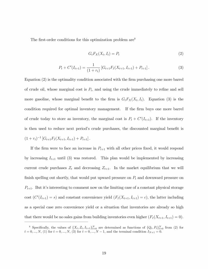
The first-order conditions for this optimization problem are8

GtFX(Xt, It) = Pt (2)

Pt + C 0(It+1) =1

(1+ rt)[Gt+1FI(Xt+1, It+1) + Pt+1] . (3)

Equation (2) is the optimality condition associated with the firm purchasing one more barrel

of crude oil, whose marginal cost is Pt, and using the crude immediately to refine and sell

more gasoline, whose marginal benefit to the firm is GtFX(Xt, It). Equation (3) is the

condition required for optimal inventory management. If the firm buys one more barrel

of crude today to store as inventory, the marginal cost is Pt + C 0(It+1). If the inventory

is then used to reduce next period’s crude purchases, the discounted marginal benefit is

(1+ rt)−1 [Gt+1FI(Xt+1, It+1) + Pt+1] .

If the firm were to face an increase in Pt+1 with all other prices fixed, it would respond

by increasing It+1 until (3) was restored. This plan would be implemented by increasing

current crude purchases Zt and decreasing Zt+1. In the market equilibrium that we will

finish spelling out shortly, that would put upward pressure on Pt and downward pressure on

Pt+1. But it’s interesting to comment now on the limiting case of a constant physical storage

cost (C 0(It+1) = s) and constant convenience yield (FI(Xt+1, It+1) = c), the latter including

as a special case zero convenience yield or a situation that inventories are already so high

that there would be no sales gains from building inventories even higher (FI(Xt+1, It+1) = 0).

8 Specifically, the values of Xt, Zt, It+1Nt=0 are determined as functions of Qt, PtNt=0 from (2) fort = 0, ..., N, (1) for t = 0, ..., N, (3) for t = 0, ..., N − 1, and the terminal condition IN+1 = 0.

19

In this case (3) becomes

Pt + s =1

(1+ rt)[Gt+1c+ Pt+1] . (4)

In this limiting case, (4) becomes an equilibrium condition that would have to characterize

the relation between Pt and Pt+1 in any equilibriumwith nonzero inventories. If, for example,

the right-hand side of (4) exceeded the left, there would be an infinite increase in the demand

for crude Zt and infinite decrease in Zt+1, to which the equilibrium prices Pt and Pt+1 would

have to respond until the equality (4) was restored.

More generally, if C 0(It) and FI(Xt, It) are relatively flat functions of It, then the effect of

(3) is to force Pt and Pt+1 to move closely together. In crude oil markets, the futures price

Pt+1 serves an information discovery role, with any changes in the futures price translating

instantaneously into a corresponding movement in spot prices. For example, Figure 12

plots f1d, the price of crude oil for the nearest-term futures contract on day d, and f3d, the

price of oil for the futures contract expiring two months after the expiration of the contract

associated with f1d. The two series move very closely together. For 93% of the 6,421

business days between April 5, 1983 and November 12, 2008, f1d and f3d changed in the

same direction from the previous day. A regression of ∆ ln f3d on ∆ ln f1d has an R2 of 0.86.

Thus this part of Masters’ claim— that if speculation affected the futures price, the spot price

would be forced to move with it— is very much consistent with both theory and evidence.

We can close the model by specifying that crude oil is exogenously supplied,

Zt = Zt, (5)

20

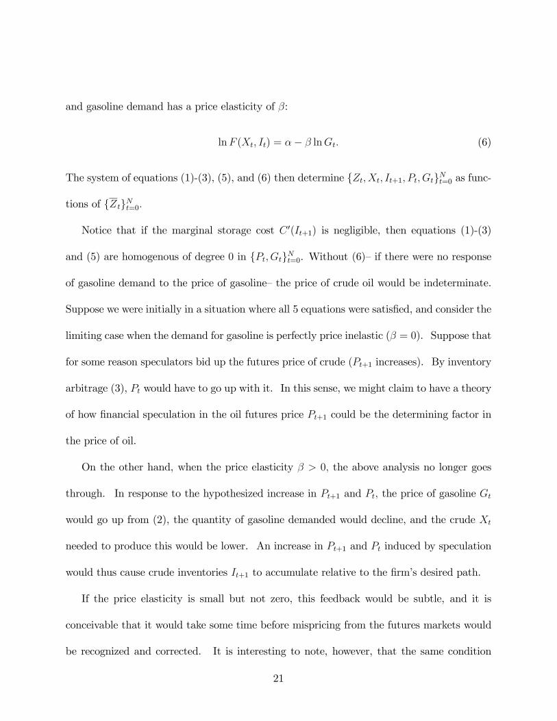
and gasoline demand has a price elasticity of β:

lnF (Xt, It) = α− β lnGt. (6)

The system of equations (1)-(3), (5), and (6) then determine Zt, Xt, It+1, Pt, GtNt=0 as func-

tions of ZtNt=0.

Notice that if the marginal storage cost C 0(It+1) is negligible, then equations (1)-(3)

and (5) are homogenous of degree 0 in Pt, GtNt=0. Without (6)— if there were no response

of gasoline demand to the price of gasoline— the price of crude oil would be indeterminate.

Suppose we were initially in a situation where all 5 equations were satisfied, and consider the

limiting case when the demand for gasoline is perfectly price inelastic (β = 0). Suppose that

for some reason speculators bid up the futures price of crude (Pt+1 increases). By inventory

arbitrage (3), Pt would have to go up with it. In this sense, we might claim to have a theory

of how financial speculation in the oil futures price Pt+1 could be the determining factor in

the price of oil.

On the other hand, when the price elasticity β > 0, the above analysis no longer goes

through. In response to the hypothesized increase in Pt+1 and Pt, the price of gasoline Gt

would go up from (2), the quantity of gasoline demanded would decline, and the crude Xt

needed to produce this would be lower. An increase in Pt+1 and Pt induced by speculation

would thus cause crude inventories It+1 to accumulate relative to the firm’s desired path.

If the price elasticity is small but not zero, this feedback would be subtle, and it is

conceivable that it would take some time before mispricing from the futures markets would

be recognized and corrected. It is interesting to note, however, that the same condition

21

needed to rationalize a speculation-based interpretation of the oil shock of 2007-08— a very

low price elasticity of oil demand— is exactly the same condition that would enable us to

attribute the event to fundamentals alone.

The other possible way in which advocates of the price bubble interpretation might at-

tempt to reconcile their story with the physical side of the petroleummarket is to hypothesize

a mechanism whereby the quantity of oil supplied Zt is itself influenced by the futures price.

Given the pressures for growth in petroleum demand from countries like China to continue,

if it remains difficult to increase global production, the price pressures of 2008 are only the

beginning of the story. Recalling the Hotelling (1931) principle, it would in this situation

pay the owners of the resource to forego current production, in order to be able to sell the

oil at the higher future price. One might then argue that oil producing countries were

misled by the speculative purchases of oil futures contracts into reducing current production

Zt in response, by this mechanism reconciling the postulated speculation with the physical

dynamics of oil supply and demand (1); for more discussion see Jovanovic (2007).

If so, such miscalculation by oil producers could not have been based on comparing the

longer-term futures price with the spot price available in 2008. Figure 13 plots the term

structure of prices implied by New York Mercantile Exchange futures contracts at the height

achieved by oil prices in July 2008. Although there was a modest upward slope in the

very near-term contracts (for example, the December 2008 contract sold for a higher price

than August 2008), that slope turned distinctly downward after the February 2009 contract,

meaning that any producers who used the futures contracts to sell their oil forward could plan

22

on selling future production at a lower price than current production. This downward slope

from 2009 onward is inconsistent with a natural Hotelling interpretation of why producers

might keep oil in the ground. Notwithstanding, one might argue that producers distrusted

the futures markets, and could not use them as a significant hedge given the volumes. Ex

post, the high spot price in 2008 meant that a country that had held off production from

2001 to 2008 would have been richly rewarded, which experience might persuade some of

the benefits of not producing all out in 2008, either. Of interest is this report from Reuters

news service on April 13, 2008:

Saudi Arabia’s King Abdullah said he had ordered some new oil discoveries left

untapped to preserve oil wealth in the world’s top exporter for future generations,

the official Saudi Press Agency (SPA) reported.

“I keep no secret from you that when there were some new finds, I told them,

‘no, leave it in the ground, with grace from God, our children need it’,” King

Abdullah said in remarks made late on Saturday, SPA said.

With hindsight, it is hard to deny that the price rose too high in July 2008, and that

this miscalculation was influenced in part by the flow of investment dollars into commodity

futures contracts. It is worth emphasizing, however, that the two key ingredients needed

to make such a story coherent— a low price elasticity of demand, and the failure of physical

production to increase— are the same key elements of a fundamentals-based explanation of

the same phenomenon. I therefore conclude that these two factors, rather than speculation

per se, should be construed as the primary cause of the oil shock of 2007-08. Certainly the

23

casual conclusion one might have drawn from glancing at Figure 1 and hearing some of the

accounts of speculation9 — that it was all just a mistake, and the price should have stayed

at $50/barrel throughout the period 2005-08— would be profoundly in error.

4 Consequences of historical oil shocks.

In essentially any theoretical model of the economic effects of a change in oil prices, a key

parameter is the value share such as the series plotted in Figure 3. To see why this is a

key parameter, consider for example a firm producing output Yt with inputs of capital Kt,

labor Nt, and energy Et. Suppose that the firm is operating at a point where the marginal

product of energy is equal to its relative price:

∂F (Kt, Nt, Et)

∂Et= Pt. (7)

Multiplying both sides of (7) by Et/F (Kt,Nt, Et) establishes that the elasticity of output

with respect to energy is given by the value share,

∂ lnF (Kt, Nt, Et)

∂ lnEt

= αt

for αt = PtEt/F (Kt,Nt, Et). Alternatively, consider a consumer facing a π% increase in the

relative price of energy. One short-run option available to the consumer (and indeed, given

the empirical evidence reviewed above, not a bad approximation to what actually happens)

is to continue to purchase the same quantity of energy as before. This would require the

9 For example, the Obama campaign site in June of 2008 included a number of quotes from analysts suchas Shell President John Hofmeister that the proper range of crude oil is “somewhere between $35 and $65 abarrel.” See http://www.econbrowser.com/archives/2008/06/how_big_a_contr.html for details.

24

consumer either to reduce saving or to cut spending on other items. If αt denotes the

consumer’s energy expenditure share, the requisite percentage cut in spending on other

items would be given by αtπ.

A large number of papers have investigated the economic consequences of previous oil

price shocks. Recent refinements include investigations of the following: (1) nonlinearity

in the relation, with oil price increases having a bigger effect on the economy than oil price

decreases (e.g., Hamilton, 2003); (2) the causes of the oil shock, with price increases brought

about by surging global demand having less of a disruptive effect than those caused by losses

in supply (e.g., Kilian, forthcoming); and (3) a changing relation over time, with the modern

economy more resilient to an oil price shock than it had been historically (e.g., Blanchard

and Galí, 2008).

Although these issues are unquestionably quite important, it is useful to look first at

some simple linear representations of the basic correlations in the historical data, with a

minor automatic adjustment for one source of a possible changing impact over time due

to the changes in αt. This is the approach taken by Edelstein and Kilian (2007). They

estimated monthly bivariate autoregressions of the form

xt = k1 +6X

s=1

φ11xt−s +6X

s=1

φ12yt−s + ε1t

yt = k2 +6X

s=1

φ21xt−s +6X

s=1

φ22yt−s + ε2t

where yt is a macro variable of interest and xt is the change in relative energy prices weighted

25

by the expenditure share,

xt = αt(lnPt − lnPt−1)

for αt the series plotted in Figure 3 and Pt the ratio of the personal consumption expenditure

deflator for energy goods and services to the overall PCE deflator. Thus for example a

unit shock to xt would result if there were a monthly 20% increase in relative energy prices

(lnPt− lnPt−1 = 0.20) at a time when energy consumed 5% of household budgets (αt = 5.0).

A unit shock to xt means that households would suffer a 1% loss in ability to purchase non-

energy items if they attempted to hold real energy consumption fixed following a shock of

size xt = 1.

I re-estimated a number of the Edelstein-Kilian regressions for the sample period they

used (with the dependent variable running from 1970:M7 through 2006:M7), and first report

the results for yt = 100(lnYt − lnYt−1) with Yt real personal consumption expenditures.

Figure 14 reproduces their orthogonalized impulse-response functions (with energy prices xt

ordered first) for the cumulative consequences for the levels Xt =Pt

j=1 xt and 100 lnYt of a

unit shock to xt−s. The first panel shows that there is relatively little serial correlation in

the energy price change series xt. Almost all of the price consequences appear within the

first two months— if xt increases by one unit at time t, one would typically expect another

0.5 move up at t+ 1, with very minor subsequent adjustments resulting in an eventual 1.7%

cumulative loss in purchasing power as a result of a unit shock to xt.

The second panel shows the decline in real consumption expenditures following historical

energy price increases. There are two aspects of this graph that are not what one would have

26

expected from the simple expenditure-impact effect sketched above. The first is the mag-

nitude of the response— following a decline that eventually would have reduced consumers’

ability to purchase non-energy items by 1.7%, we observe that on average consumers in fact

eventually cut their spending by 2.2%. Why should consumption spending fall by even

more than the predicted upper bound? The second surprising aspect concerns the timing—

although the price moves immediately reduce purchasing power, the biggest declines in total

spending don’t come until 6 months or more after the initial shock.

One way that Edelstein and Kilian sought to explain these anomalies is by breaking

down the responses in terms of the various components of consumption. Figure 15 re-

produces their findings for Yt corresponding respectively to the services, nondurables, and

durables components of real personal consumption expenditures. The magnitude of the

first two responses is in line with the simple expenditure-share effects, while the response of

expenditures on durable goods is five times as big.

The first panel of Figure 16 looks in particular at the motor vehicles component of

durables. In contrast to the gradual response one sees in broader consumption categories,

here the response is immediate and quite huge, with for example a 20% increase in energy

prices in an environment with an energy expenditure share of 5% resulting in a 10% decrease

in spending on motor vehicles. That there would be a direct link between such spending

and energy prices is quite plausible, and its mechanism comes not from the simple budget-

constraint effect. Indeed, for this category of spending there are a number of other factors

that are much more important, such as postponing the purchase of a new vehicle until better

27

information about where gas prices are going to end up is available and shifting the purchase

from bigger to more fuel efficient (and perhaps less expensive) vehicles.

If we take it as given that there are big and immediate effects on purchases of items such

as motor vehicles, both the delayed response and the multiplier effect on other categories of

spending can also be better understood. The shift in spending means a reduction in income

for those employed in manufacturing and selling cars. Given the significant technological

frictions in relocating the now underutilized labor and capital to other sectors, the result is

a decline in aggregate income and a loss in purchasing power over and above that caused by

the initial price increase itself (Hamilton, 1988).

The second panel of Figure 16 presents a second effect identified by Edelstein and Kilian

that is huge and immediate— a drop in consumer sentiment.10 For whatever reason,

consumers found the historical oil shocks to be very troubling events, with a 20% increase

in relative energy prices (assuming again a base case value share of αt = 5) producing a

15-point drop in the index of consumer sentiment. One can argue whether a response

of this magnitude is rational given the size of the shock. The budget consequences of

spiking gasoline prices are something consumers experience immediately, and represent an

aggregate event that forces everybody to make changes at the same time. Certainly if your

job is related to the auto industry (or if you perceive that what happens to them will have

eventual implications for your own job security), it’s quite rational to view these events as

10 Note that unlike the previous figures in which the second variable in the VAR, yt = 100(lnYt− lnYt−1)represented a rate of change (with impulse-response graphs subsequently translated back into implicationsfor the levels 100 lnYt), in the second panel of Figure 16, the variable yt is the level of the index of consumersentiment itself and the graph shows the consequences for yt+s following a unit shock to xt.

28

carrying pessimistic implications beyond the immediate loss in spending power. In any

case, the changes in sentiment that we find in the data could easily have made a significant

contribution to the subsequent path of both consumption and investment spending.

Suppose we stick just to the narrowest effect of the energy price shock, namely changes in

spending on motor vehicles and parts. How big a contribution would this alone have made

to the subsequent economic downturns, ignoring any possible multiplier effects? The first

column of Table 3 reports the actual average growth rate of real GDP over the 5 quarters

following each of the 4 historical oil shocks discussed here. All of these episodes— in which

GDP fell on average over a period of 5 quarters— are included in the list of U.S. economic

recessions. The second column does a very simple calculation, asking what the average

GDP growth would have been if there had been zero change in the motor vehicles and

parts component of GDP over these 5 quarters, with all other components of GDP staying

the same as reported.11 Although this is a modest contribution (less than 0.8% in any

episode), it is enough to move the average from negative to positive territory in the case of

the 1980 and 1990-91 recessions, offering some basis for thinking that, had it not been for

the significant downturn in autos in each of these episodes, they might have been regarded

as episodes of sluggish growth rather than clear recessions. By contrast, in the more serious

1973-75 and 1981-82 recessions, there was clearly something more significant than just autos

bringing down the economy.

11 This was calculated by subtracting from the growth rate of real GDP the contribution of motor vehiclesand parts as reported in Table 1.5.2 from the Bureau of Economic Analysis. Note that this contribution isa negative number in each episode, so that subtracting it would make the GDP growth rate bigger.

29

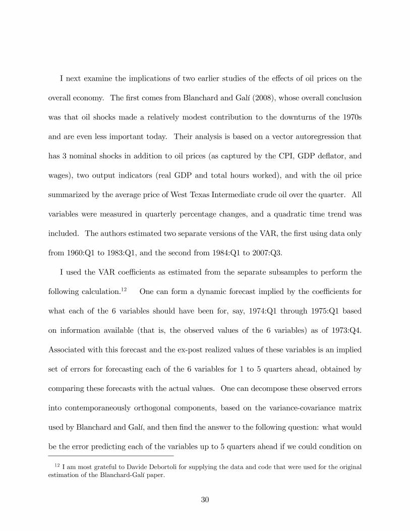
I next examine the implications of two earlier studies of the effects of oil prices on the

overall economy. The first comes from Blanchard and Galí (2008), whose overall conclusion

was that oil shocks made a relatively modest contribution to the downturns of the 1970s

and are even less important today. Their analysis is based on a vector autoregression that

has 3 nominal shocks in addition to oil prices (as captured by the CPI, GDP deflator, and

wages), two output indicators (real GDP and total hours worked), and with the oil price

summarized by the average price of West Texas Intermediate crude oil over the quarter. All

variables were measured in quarterly percentage changes, and a quadratic time trend was

included. The authors estimated two separate versions of the VAR, the first using data only

from 1960:Q1 to 1983:Q1, and the second from 1984:Q1 to 2007:Q3.

I used the VAR coefficients as estimated from the separate subsamples to perform the

following calculation.12 One can form a dynamic forecast implied by the coefficients for

what each of the 6 variables should have been for, say, 1974:Q1 through 1975:Q1 based

on information available (that is, the observed values of the 6 variables) as of 1973:Q4.

Associated with this forecast and the ex-post realized values of these variables is an implied

set of errors for forecasting each of the 6 variables for 1 to 5 quarters ahead, obtained by

comparing these forecasts with the actual values. One can decompose these observed errors

into contemporaneously orthogonal components, based on the variance-covariance matrix

used by Blanchard and Galí, and then find the answer to the following question: what would

be the error predicting each of the variables up to 5 quarters ahead if we could condition on

12 I am most grateful to Davide Debortoli for supplying the data and code that were used for the originalestimation of the Blanchard-Galí paper.

30

the ex post realizations of the innovations in oil prices, but did not know anything else?13

On the basis of this number, I calculated what the average GDP growth over 1974:Q1-75:Q1

would have been had there been no oil price shock but the other 5 shocks to the CPI, deflator,

wages, GDP, and hours had been identical to the realized historical residuals. The answer

to that “what if” question is reported in the third column of Table 3. The Blanchard-Galí

estimates imply that, had there been no oil shock, the severe downturn of 1973-75 would

have been only a very mild recession. Interestingly, although their estimated post-1984

effects of oil prices are much smaller than those for their earlier sample, and although the

authors did not single out the aftermath of the First Gulf War as a separate oil shock, their

estimates also imply that, had the price of oil not spiked following Iraq’s invasion of Kuwait,

the U.S. might have avoided the 1990-91 recession.

Surprisingly, the Blanchard-Galí estimates imply that the 1981-82 downturn would actu-

ally have been more severe in the absence of disturbances to oil prices. This is because the

measure they used for the price of oil, the price of WTI, actually fell between July 1980 and

March 1981. Other indicators, however, suggest a very different story. For example, the

13 Mathematically, the estimated VAR coefficients imply a set of moving average matrices Ψs (as inequation [10.1.19] in Hamilton, 1994), and the Cholesky factor of the residual variance matrix can be obtainedas Ω = PP

0. The s-step-ahead forecast error can then be written

yt+s − yt+s|t−1 = ²t+s + Ψ1²t+s−1 + . . .+ Ψsεt

for εt the implied one-step-ahead forecast errors. Define the orthogonalized residuals by vt = P−1εt andlet p1 denote the first column of P. Then the contribution of v1t, v1,t+1, ..., v1,t+s to this forecast erroris calculated as

Psk=0 Ψkp1v1,t+s−k, and the calculation of what the value of yt+s would have been in the

absence of the oil shocks is calculated as yt+s −Ps

k=0 Ψkp1v1,t+s−k. Note that although the VAR shocksto oil prices and the CPI are correlated in the data (ε1t is correlated with ε2t), the shocks v1t and v2t areorthogonal in the sample by construction. Thus when we ask what would have happened if v1t had beenzero but v2t had been as observed historically, we are implicitly subtracting out that movement in the CPIthat is correlated statistically with the oil price, and leaving in other, uncorrelated factors.

31

EIA’s series for the refiner acquisition cost (the series plotted in the row 3, column 2 panel

of Figure 5) shows a 27% (logarithmic) increase over this same period, the BLS’s producer

price index for crude petroleum (the series used by Hamilton, 1983 and 2003) shows a 42%

increase, the BEA’s implicit price deflator for consumption expenditures on energy goods

and services (the series used by Edelstein and Kilian, 2007) shows a 12% increase, and the

BLS’s consumer price index for gasoline shows an 11% increase. It therefore seems likely

that, despite the results implied by Blanchard and Galí’s estimation, energy prices were a

factor reducing GDP growth over this episode along with the others.

As another comparison, I turned to the nonlinear specification investigated in Hamilton

(2003), whose key result (equation 3.8) was a regression of quarterly real GDP growth on a

constant, 4 of its own lags, and 4 lags of the “net oil price increase”, defined as the percentage

change in the crude oil PPI during the quarter if oil prices made a new 3-year high at the

time, and zero if oil prices ended the quarter lower than a point they had reached over the

previous 3 years. The coefficients for that relation, estimated over t = 1949:Q2 through

2001:Q3 were as follows

yt = 0.98(0.13)

+ 0.22(0.07)

yt−1 + 0.10(0.07)

yt−2 − 0.08(0.07)

yt−3 − 0.15(0.07)

yt−4 (8)

− 0.024(0.014)

o#t−1 − 0.021(0.014)

o#t−2 − 0.018(0.014)

o#t−3 − 0.042(0.014)

o#t−4.

To get a sense of the magnitudes implied by these coefficients,14 I calculated for each quarter

in the episode the difference between the 1-quarter-ahead forecast implied by equation (8),

14 One could in principle find the answer to an s-period-ahead forecasting equation as in footnote 13,though this would require a specification of the dynamic path followed by the net oil price increase variable.No such specification was proposed in Hamilton (2003), and it seems unlikely that spelling one out wouldchange the results significantly from the simpler calculation provided here.

32

and what that 1-quarter-ahead forecast would have been if the oil price measure o#t−1, ..., o#t−4

had instead been equal to zero, and took this difference as a measure of the contribution

of the oil shock to that quarter’s real GDP growth. From the fourth column of Table 3,

it appears that this specification would attribute almost all of the deviation from trend in

each of the four recessions to the oil shock alone.

To summarize, there is a range of estimates available as to the size of the contribution

that oil shocks have made to historical U.S. recessions. But even the most modest estimates

support the claim that the oil shocks made a significant contribution in at least some of

these episodes. My conclusion is that, had the oil shocks not occurred, GDP would have

grown rather than fallen in at least some of these episodes.

5 Consequences of the oil shock of 2007-08.

Let us begin by examining what happened to motor vehicle sales in response to the price

changes noted in Figure 6. Figure 17 reports sales in the U.S. of domestically manufactured

light vehicles broken down in terms of cars versus light trucks. The latter include the sport

utility vehicle (SUV) category, which up until 2007 had been outselling cars in the U.S.

market. Beginning in 2008, sales of SUVs began to plunge, and were down more than

25% relative to the preceding year in May, June and July. SUV sales rebounded somewhat

when gas prices began to fall in August, only to suffer a second hit in September through

December.

To what extent was the decline in SUV sales in the first half of 2008 caused by rising

33

gasoline prices as opposed to falling income? One measure relevant for addressing this

question is the contrast between the sales of light trucks (top panel of Figure 17) and those

of cars (bottom panel). A general drop in income would affect both categories, whereas

the effects of rising gasoline prices would hit light trucks much harder than cars. In the

event, domestic car sales were only down on average by 7% in May, June, and July 2008

compared with the same months in 2007. Even more dramatic are the comparisons for

imports. Imported cars were up 10% over these same three months (bottom panel of Figure

18). Sales of imported light trucks (top panel of Figure 18), by contrast, were down 22%.

Thus the dominant story in the first half of 2008 was one in which American consumers were

switching from SUVs to smaller cars and more fuel-efficient imports.

Although gasoline prices were likely a key factor behind plunging sales for U.S. automak-

ers in the first half of 2008, falling income appears to be the biggest factor driving sales back

down in the fourth quarter of 2008. Here we see, in contrast to the first half of 2008, the

sales decline was across the board, hitting cars if anything more than SUVs, and imports

along with domestics.

The result was a significant shock to the U.S. auto industry in 2008:H1, quite comparable

in magnitude to what was observed in the wake of the oil shock of 1990. The contribution

of motor vehicles and parts to U.S. real GDP (measured in 2000 dollars at an annual rate)

was $30 billion smaller in 1991:Q1 than it had been in 1990:Q3, similar to the $34 billion

decline in this sector between 2007:Q4 and 2008:Q2 (BEA Table 1.5.6). Granted, that $34

billion in 2007-08 represents a smaller share of total GDP than did the lost auto production

34

in 1990-91, but the most recent slump still represents a sizable number, and it would be hard

to defend the claim that a recession began in 2007:Q4 had it not been for the contribution

from the auto sector. The first two columns of Table 3 include details on this breakdown,

looking ahead either 4 or 5 quarters beginning with 2007:Q4. Focusing first on just the four

quarters 2007:Q4-2008:Q3, average real GDP growth over this period was actually +0.75%

at an annual rate. Had there been no decline in autos, that number would have been nearly

half a percentage point higher. It would be very hard to characterize 2007:Q4-2007:Q3

as a full year of recession, had the average growth indeed been +1.2%. The Business

Cycle Dating Committee of the National Bureau of Economic Research reported that it was

looking not just at GDP (which even with the decline in autos showed clearly positive overall

growth), but also at gross domestic income, which differs from GDP only by a statistical

discrepancy; (see Nalewaik, 2007). GDI growth averaged -0.4% over this period, offering

more justification for the NBER’s recession call. But again, without the hit to autos, this

number instead would also have registered positive, albeit very anemic, growth.

The 2007-08 shock was also comparable to 1990-91 in terms of the effect on employment in

the automobile industry. Seasonally adjusted manufacturing employment in motor vehicles

and parts fell by 94 thousand workers between 1990:M7 and 1991M3, whereas it fell by 125

thousand between 2007:M7 and 2008:M8 (BLS series CES3133600101). Again the latter is

relative to a larger economy, but again it is not an inconsequential number. A year-over-year

drop in total employment is viewed by some as a defining characteristic of a U.S. recession.

This threshold was crossed in June 2008, when 8,000 fewer workers were employed compared

35

with June 2007. Again without the contribution of autos, it would not be at all clear that the

U.S. economy should have been characterized as being in recession during 2007:Q4-2008:Q2.

Of course, the first half of 2008 saw not just a big decline in automobile purchases but also

a slowdown in overall consumer spending and a big drop in consumer sentiment, again very

much consistent with what was observed after other historical oil shocks. Like SUV sales,

consumer sentiment spiked back up dramatically in an initial response to falling gasoline

prices at the end of the summer, but, like SUV sales, then plunged back down as broader

economic malaise developed in the fall of 2008.

For some more formal statistical evidence and quantification, I turn to several of the

studies described in the previous section. I first examine in Table 4 how well the models

proposed in previous studies have performed in terms of describing data that have arrived in

the time since those papers were written. To evaluate the Edelstein-Kilian bivariate VARs,

I used the parameter values for the relations as estimated over 1970:M7-2006:M7 to form

forecasts over the post-sample interval 2006:M8-2008:M9. I compared those post-sample

one-month-ahead mean squared errors with the MSEs that would have been obtained by a

univariate autoregression (excluding energy prices) estimated over the same original sample

(1970:M7-2006:M7). As reported in the last column of Table 4, for each of the 6 Edelstein-

Kilian relations used here, energy prices made a useful contribution to the post-sample

forecasts, giving us some confidence in using those estimates to measure the contribution

that energy prices may have made to what happened to the economy in response to the oil

shock of 2007-08.

36

I used the Edelstein-Kilian relations as estimated over 1970:M7-2006:M7 to form a 1- to

12-month-ahead forecast of how these variables might have behaved over 2007:M9 through

2008:M9 had there been no oil shock. The top panel of Figure 19 presents the results for real

personal consumption expenditures. The dotted line represents the forecast of the model

for PCE over these 12 months. In the absence of any new shocks, the Edelstein-Kilian

bivariate VAR would have predicted consumption to continue growing at the rate it had

over the previous half year. In the event, actual consumption (the solid line) grew much

more slowly than predicted through May and then started to decline. The dashed line

represents the portion of the forecast error at any date that could be accounted for by the

cumulative surprises in energy prices between 2007:M9 and the indicated date, calculated

as described in footnote 13. Energy prices can account for about half of the gap between

predicted and actual consumption spending over this period. The second and third panels

repeat the exercise for the big drops in spending on motor vehicles and consumer sentiment.

Most of the declines in these two series through the beginning of 2008 and about half the

decline through the summer of 2008 would be attributed to energy prices according to the

Edelstein-Kilian regressions.

I also examined the post-sample performance of the Blanchard-Galí VAR as estimated

over their second subsample, 1984:Q1-2007:Q3. In this case I compared their 6-variable

VAR with a 5-variable VAR that leaves out oil prices. Their model with oil prices in fact

does somewhat worse at predicting GDP growth rates for data that appeared subsequent

to their study than would a similar VAR without oil prices; (see the third row from the

37

bottom of Table 4). I nevertheless examined how much of the downturn of 2007-08 their

coefficients would attribute to oil prices, looking at the errors made forecasting GDP growth

over 2007:Q4 to 2008:Q3 or Q4 on the basis of information available as of 2007:Q3, and at

the contribution of oil price surprises to these forecast errors. The result of this calculation

(reported in the third column of Table 3) suggests that real GDP growth would have been

0.7% higher on average in the absence of the oil shock. Thus, the Blanchard-Galí calcula-

tions also support the conclusion that the period 2007:Q4-2008:Q3 would not reasonably be

considered to have been the beginning of a recession had there been no contribution from

the oil shock.

Finally, I looked at the post-sample performance of the GDP-forecasting regression (8)

estimated by Hamilton (2003). As seen in the next-to-last row of Table 4, this relation has

about the same mean squared error over the period 2001:Q4-2008:Q4 as does a univariate

AR(4) fit to the 1949:Q2-2001:Q3 data. In part this lack of improvement is due to the

fact that the oil-based relation predicts slower GDP growth than was observed for 2005 and

2006, when the price of oil rose but the U.S. economy seemed to be little affected.

It is interesting to note that the historical relation (8) significantly outperforms a uni-

variate specification when evaluated on the same post-sample intervals used to evaluate the

Edelstein-Kilian and Blancard-Galí relations in Table 4. Equation (8) has a 45% improve-

ment in terms of the post-sample MSE over the period 2007:Q1-2008:Q4 compared with a

univariate autoregression. Indeed, the relation could account for the entire downturn of

2007-08; (see the last column of Table 3). If one could have known in advance what hap-

38

pened to oil prices during 2007-08, and if one had used the historically estimated relation (8)

to form in a 1- to 5-quarter-ahead forecast of real GDP looking ahead to 2007:Q4 through

2008:Q4 from 2007:Q3, one would have been able to predict the level of real GDP for both

of 2008:Q3 and 2008:Q4 quite accurately; (see Figure 20).

That last claim seems hard to believe, since Blanchard and Galí are doubtless correct

that there has been some decrease in the effects of oil prices as the economy has become

less manufacturing-based and more flexible, and since the housing downturn surely made

a critical contribution to the recession of 2007-08. Nevertheless, a few points about the

respective contributions of housing and the oil shock deserve mentioning. I would note first

that housing had been exerting a significant drag on the economy before the oil shock, de-

spite which economic growth continued. Residential fixed investment subtracted an average

of 0.94% from the average annual GDP growth rate over 2006:Q4-07:Q3, when the economy

was not in a recession, but subtracted only 0.89% over 2007:Q4-2008:Q3, when the recession

began. At a minimum it is clear that something other than housing deteriorated to turn

slow growth into a recession. That something, in my mind, includes the collapse in auto-

mobile purchases, slowdown in overall consumption spending, and deteriorating consumer

sentiment, in which the oil shock was indisputably a contributing factor.

Second, there is an interaction effect between the oil shock and the problems in housing.

Cortright (2008) noted that in the Los Angeles, Tampa, Pittsburgh, Chicago, and Portland-

Vancouver Metropolitan Statistical Areas, house prices in 2007 were likely to rise slightly

in the zip codes closest to the central urban areas but fall significantly in zip codes with

39

longer average commuting distances. Foreclosure rates also rose with distance from the

center. And certainly to the extent that the oil shock made a direct contribution to lower

income and higher unemployment, that would also depress housing demand. For example,

the estimates in Hamilton (2008) imply that a 1% reduction in real GDP growth translates

into a 2.6% reduction in the demand for new houses.

Eventually, the declines in income and house prices set mortgage delinquency rates be-

yond a threshold at which the overall solvency of the financial system itself came to be

questioned, and the modest recession of 2007:Q4-2008:Q3 turned into a ferocious downturn

in 2008:Q4. Whether we would have avoided those events if the economy had not gone

into recession, or instead would have merely postponed them, is a matter of conjecture.

Regardless of how we answer that question, the evidence to me is persuasive that, if there

had there been no oil shock, we would have described the U.S. economy in 2007:Q4-2008:Q3

as growing slowly, but not in a recession.

Lastly I take up the question of why the oil price increases prior to 2007:Q4 failed to

have a bigger effect on the economy. Why did consumers respond so little when the price of

oil went from $41/barrel in July 2004 to $65 in August 2005 (a 59% increase), and yet were

observed to have such a big response to the increase from $72 in August 2007 to $134 (an

86% increase) in June 2008?15 Equations posed in terms of percentage changes, such as

(8), would predict that the 2004-2005 price increases should also have had significant effects

on output. However, in terms of the dollar impact on household budgets, the $62/barrel

15 Oil prices quoted here are monthly averages of daily West Texas Intermediate prices.

40

price increase in 2007-08 is considerably more than twice as significant as the $24/barrel

increase in 2004-2005.

To explore this possibility more concretely, I looked at the consequences of modifying

equation (8) to take into account the changes in the energy budget share over time, replacing

o#t with the product o#t αt−1 for αt the energy share plotted in Figure 3.16 This results in a

slight improvement in fit for the original sample period (t = 1949:Q2 to 2001:Q3), raising the

log likelihood from -281.78 for the original specification to -281.47 for the new. The share-

weighted regression has a significantly better post-sample performance, producing a 10.8%

improvement in the MSE over the period 2001:Q4-2008:Q4 relative to an autoregression with

no role for oil prices. For the specific years 2005:Q1-2006:Q4, the modified specification as

estimated over 1949:Q2 to 2001:Q3 would have predicted an average annual real GDP growth

rate of 1.9%, a bit below the sluggish 2.5% that was actually observed.

Oil prices thus appear to have exerted a moderate drag on real GDP in 2005-2006 and

made a more significant negative contribution in 2007-2008. The principle reason that

Americans ignored the earlier price increases would seem to be because they could afford to

do so. By 2007:Q4, they no longer could, and the sharp spike in oil prices led to an observed

economic response similar to what we had seen in earlier episodes.

16 The monthly series was converted to quarterly by using the third month of the quarter. Values for αtfor t prior to 1959:Q1 were simply set equal to the January 1959 value (7.354).

41

6 Policy implications.

I have raised the possibility that miscalculation of the long-run price elasticity of oil demand

by market participants was one factor behind the oil shock of 2007-08, and that speculative

investing in oil futures contracts may have contributed to that miscalculation. Were any

policies available to mitigate this? One option to consider would have been for the U.S.

government to sell some oil directly out of the Strategic Petroleum Reserve in the spring of

2008, perhaps timing the sales to coincide with the NYMEX crude contract expiry dates.

If there was speculative momentum buying, such steps might have succeeded in reversing

it. If not, the worst would be that the government made a profit on its SPR investment by

buying low and selling high.

A more conventional policy tool would be monetary policy. A number of observers

suggested that the very rapid declines of short-term interest rates in 2008:Q1 fanned the

flames of commodity speculation, with negative real interest rates encouraging investments

in physical commodities (e.g., Frankel, 2008). In January 2009, Federal Reserve Chair Ben

Bernanke offered the following retrospective on that debate:

The [Federal Open Market] Committee’s aggressive monetary easing was not

without risks. During the early phase of rate reductions, some observers ex-

pressed concern that these policy actions would stoke inflation. These concerns

intensified as inflation reached high levels in mid-2008, mostly reflecting a surge

in the prices of oil and other commodities. The Committee takes its responsi-

bility to ensure price stability extremely seriously, and throughout this period

42

it remained closely attuned to developments in inflation and inflation expecta-

tions. However, the Committee also maintained the view that the rapid rise in

commodity prices in 2008 primarily reflected sharply increased demand for raw

materials in emerging market economies, in combination with constraints on the

supply of these materials, rather than general inflationary pressures. Committee

members expected that, at some point, global economic growth would moderate,

resulting in slower increases in the demand for commodities and a leveling out in

their prices—as reflected, for example, in the pattern of futures market prices. As

you know, commodity prices peaked during the summer and, rather than level-

ing out, have actually fallen dramatically with the weakening in global economic

activity. As a consequence, overall inflation has already declined significantly

and appears likely to moderate further.

Bernanke seemed here to be taking the position that since the Fed got the long run cor-

rect (ultimately there would be a significant downturn in both the economy and commodity

prices, with strong disinflationary pressure), the short-run consequences (booming commod-

ity prices in 2008:H1) were less relevant. On the other hand, if it is indeed the case that

the spike in oil prices was one causal factor contributing to the downturn itself, the Fed can

hardly afford to ignore those short-run implications. The evidence examined here suggests

that the Fed needs to give careful consideration to the possible consequences of its actions

for relative commodity prices.

But while the question of the possible contribution of speculators and the Fed is a very

43

interesting one, it should not distract us from the broader fact: some degree of significant

oil price appreciation during 2007-08 was an inevitable consequence of booming demand and

stagnant production. It is worth emphasizing that this is fundamentally a long-run problem,

which has been resolved rather spectacularly for the time being by a collapse in the world

economy. However, the economic collapse will hopefully prove to be a short-run cure for the

problem of excess energy demand. If growth in the newly industrialized countries resumes at

its former pace, it would not be too many more years before we find ourself back in the kind

of calculus that was the driving factor behind the problem in the first place. Policy-makers

would be wise to focus on real options for addressing those long-run challenges, rather than

blame what happened last year entirely on a market aberration.

44

ReferencesAl-Sowayegh, Abdulaziz H. 1984. Arab Petropolitics. London : Croom Helm.

Barsky, Robert B., and Lutz Kilian. 2002. “Do We Really Know that Oil Caused the

Great Stagflation? A Monetary Alternative." In Ben Bernanke and Kenneth Rogoff (eds.),

NBER Macroeconomics Annual 2001, pp. 137-183.

Blanchard, Olivier J., and Jordi Galí. 2008. “The Macroeconomic Effects of Oil Price

Shocks: Why are the 2000s so Different from the 1970s?” In Jordi Galí and Mark Gertler

(eds.), International Dimensions of Monetary Policy, University of Chicago Press (Chicago,

IL).

Bernanke, Ben S. 2009. “The Crisis and the Policy Response,” Stamp Lecture, Jan-

uary 13, London School of Economics, http://www.federalreserve.gov/newsevents/speech/

bernanke20090113a.htm.

Blinder, Alan S., and Jeremy B. Rudd. 2008. “The Supply-Shock Explanation of the

Great Stagflation Revisited," NBER Working Paper No. 14563.

Brons, Martijn Brons, Peter Nijkamp, Eric Pels, and Piet Rietveld. 2008. “A Meta-

Analysis of the Price Elasticity of Gasoline Demand: A SUR Approach,” Energy Economics

30, pp. 2105—2122.

Cooper, John C.B. 2003. “Price Elasticity of Demand for Crude Oil: Estimates for 23

Countries,” OPEC Review 27(1), pp. 1-8.

Cortright, Joe. 2008. “Driven to the Brink: How the Gas Price Spike Popped the Housing

Bubble and Devalued the Suburbs," Discussion paper, CEOs for Cities, http://www.ceosforcities.org

45

/newsroom/pr/iles/Driven%20to%20the%20Brink%20FINAL.pdf.

Dahl, Carol A. 1993. “A Survey of Oil Demand Elasticities for Developing Countries,”

OPEC Review 17(Winter), pp. 399-419.

Dahl, Carol and Thomas Sterner. 1991. “Analysing Gasoline Demand Elasticities: A

Survey,” Energy Economics 13, pp. 203-210.

Edelstein, Paul, and Lutz Kilian. 2007. “Retail Energy Prices and Consumer Expendi-

tures.” Working paper, University of Michigan.

Espey, Molly. 1998. “Gasoline Demand Revisited: An International Meta-Analysis of

Elasticities,” Energy Economics 20, pp. 273-295.

Frankel, Jeffrey A. 2008. “The Effect of Monetary Policy on Real Commodity Prices” in

John Campbell (ed.), Asset Prices and Monetary Policy, University of Chicago Press, pp.

291-327.

Gately, Dermot, and Hillard G. Huntington. 2002. “The Asymmetric Effects of Changes

in Price and Income on Energy and Oil Demand,” Energy Journal 23(1), pp. 19-55.

Graham, Daniel J., and Stephen Glaister. 2004. “Road Traffic Demand Elasticity Esti-

mates: A Review,” Transport Reviews 24(3), pp. 261—274.

Hamilton, James D. 1983.“Oil and the Macroeconomy Since World War II,” Journal of

Political Economy 91, pp. 228-248.

_____. 1988. “A Neoclassical Model of Unemployment and the Business Cycle,”

Journal of Political Economy 96, pp. 593-617.

_____. 1994. Time Series Analysis. Princeton, NJ: Princeton University Press.

46

_____. 2003. “What Is an Oil Shock?”, Journal of Econometrics 113(2), pp. 363-398.

_____. 2008. “Daily Monetary Policy Shocks and New Home Sales,” Journal of

Monetary Economics 55, pp. 1171-1190.

_____. 2009. “Understanding Crude Oil Prices.” Energy Journal, forthcoming.

Hotelling, Harold. 1931. “The Economics of Exhaustible Resources,” Journal of Political

Economy 39(2), pp. 137-75.

Hughes, Jonathan E., Christopher R. Knittel and Daniel Sperling. 2008. “Evidence of

a Shift in the Short-Run Price Elasticity of Gasoline Demand.” Energy Journal 29(1), pp.

93-114.

Jovanovic, Boyan. 2007. “Bubbles in Prices of Exhaustible Resources,”, working paper,

New York University.

Kilian, Lutz. 2008. “Exogenous Oil Supply Shocks: How Big Are They and How Much

Do They Matter for the U.S. Economy?” Review of Economics and Statistics 90(2), pp.

216-240.

_____. “Not All Oil Price Shocks Are Alike: Disentangling Demand and Supply

Shocks in the Crude Oil Market,” forthcoming, American Economic Review.

Leamer, Edward E. 2008. “What’s a Recession, Anyway?” NBER Working Paper No.

14221.

Nalewaik, Jeremy J. 2007. “Estimating Probabilities of Recession in Real Time Using

GDP and GDI.” Working paper, Board of Governors of the Federal Reserve System.

47

48

Table 1. Estimates of absolute value of short-run demand price elasticity.

Study Product Method ElasticityDahl and Sterner (1991)

gasoline literature survey 0.26

Espey (1998) gasoline literature survey 0.26 Graham and Glaister (2004)

gasoline literature survey 0.25

Brons, et. al. (2008) gasoline literature survey 0.34 Dahl (1993) oil (developing

countries) literature survey 0.07

Cooper (2003) oil (average of 23 countries)

annual time-series regression

0.05

Source: Hamilton (2009). Table 2. Sizes of quantity and prices changes in historical oil shocks. Episode Supply reduction Price change Implied elasticity Oct 73 - Mar 74 4.0% 41.3% 0.10 Nov 78 - Jul 79 1.3% 38.7% 0.03 Oct 80 - Mar 81 1.2% 25.8% 0.05 Aug 90 - Oct 90 2.9% 71.6% 0.04 Notes. Second column. Average shortfall of global production of crude petroleum over indicated period as a percent of global production the month before the indicated episode. Third column. Cumulative change in 100 times the natural log of crude oil price over the indicated episode. Data sources same as those for Figure 5. Fourth column. Ratio of second to third columns. Table 3. Average annual real GDP growth rates under alternative scenarios. Period Actual Without autos Without oil

shock (Blanchard-Gali)

Without oil shock (Hamilton)

1974:Q1-75:Q1 -2.5% -2.0% -0.1% +2.3% 1979:Q2-80:Q2 -0.4% +0.4% +0.4% +2.5% 1981:Q2-82:Q2 -1.5% -1.3% -2.0% +2.0% 1990:Q3-91:Q3 -0.1% +0.2% +0.5% +3.6% 2007:Q4-08:Q3 +0.7% +1.2% +1.4% +4.2% 2007:Q4-08:Q4 -0.7% -0.0% -0.2% +3.2%

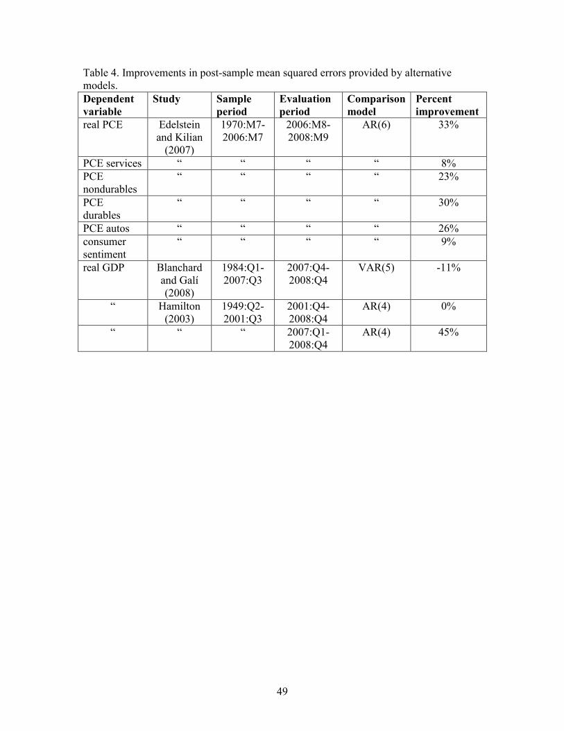
49

Table 4. Improvements in post-sample mean squared errors provided by alternative models. Dependent variable

Study Sample period

Evaluation period

Comparison model

Percent improvement

real PCE Edelstein and Kilian

(2007)

1970:M7-2006:M7

2006:M8- 2008:M9

AR(6) 33%

PCE services “ “ “ “ 8% PCE nondurables

“ “ “ “ 23%

PCE durables

“ “ “ “ 30%

PCE autos “ “ “ “ 26% consumer sentiment

“ “ “ “ 9%

real GDP Blanchard and Galí (2008)

1984:Q1-2007:Q3

2007:Q4-2008:Q4

VAR(5) -11%

“ Hamilton (2003)

1949:Q2-2001:Q3

2001:Q4-2008:Q4

AR(4) 0%

“ “ “ 2007:Q1-2008:Q4

AR(4) 45%

50

Figure 1. Real price of crude petroleum in November 2008 dollars per barrel.

0

20

40

60

80

100

120

140

1945 1955 1965 1975 1985 1995 2005

Notes. Monthly average price of West Texas Intermediate divided by ratio of consumer price index for indicated month to consumer price index for November 2008, for 1947:M1 through 2008:M12.

51

Figure 2. Logs of U.S. real GDP and oil consumption, 1949-2007.

0

0.2

0.4

0.6

0.8

1

1.2

1.4

0 0.25 0.5 0.75 1 1.25 1.5 1.75 2

GDP

Oil

1949-61: slope = 1.2

1961-73:slope = 1.04

1985-97:slope = 0.47

Notes. Horizontal axis: cumulative change in natural logarithm of U.S. real GDP between 1949 and the year for which a given data point is plotted, from Bureau of Economic Analysis Table 1.1.6. Vertical axis: cumulative change in natural logarithm of total petroleum products supplied to U.S. market between 1949 and the year for which a given data point is plotted, from Energy Information Administration, “Petroleum Overview, 1949-2007”, Table 5.1 (http://www.eia.doe.gov/emeu/aer/txt/ptb0501.html). Source: Hamilton (2009).

52

Figure 3. Dollar value of energy expenditures as a percentage of total consumer expenditures, 1959:M1-2008:M9.

1960 1965 1970 1975 1980 1985 1990 1995 2000 20050.0

2.5

5.0

7.5

10.0

Notes. Calculated as 100 times nominal monthly consumption expenditures on energy goods and services divided by total personal consumption expenditures. Data source: BEA Table 2.3.5U, “Personal Consumption Expenditures by Major Type of Product and Expenditure,” obtained from Econstats (http://www.econstats.com/nipa/ NIPA2u_2_3_6U_.htm).

53

Figure 4. Monthly oil production for Iran, Iraq, and Kuwait.

Iran

1973 1975 1977 1979 1981 1983 1985 1987 1989 1991 1993 1995 1997 1999 2001 2003 2005 20070

1000

2000

3000

4000

5000

6000

7000

Iraq

1973 1975 1977 1979 1981 1983 1985 1987 1989 1991 1993 1995 1997 1999 2001 2003 2005 20070

5001000150020002500300035004000

Kuwait

1973 1975 1977 1979 1981 1983 1985 1987 1989 1991 1993 1995 1997 1999 2001 2003 2005 20070

5001000150020002500300035004000

Notes. Monthly crude oil production, including lease condensate, in barrels per day, 1973:M1-2007:M6. Data source: Energy Information Administration, Monthly Energy Review, September 2007, Table 11.1a (http://tonto.eia.doe.gov/merquery/ mer_data.asp?table=T11.01a).

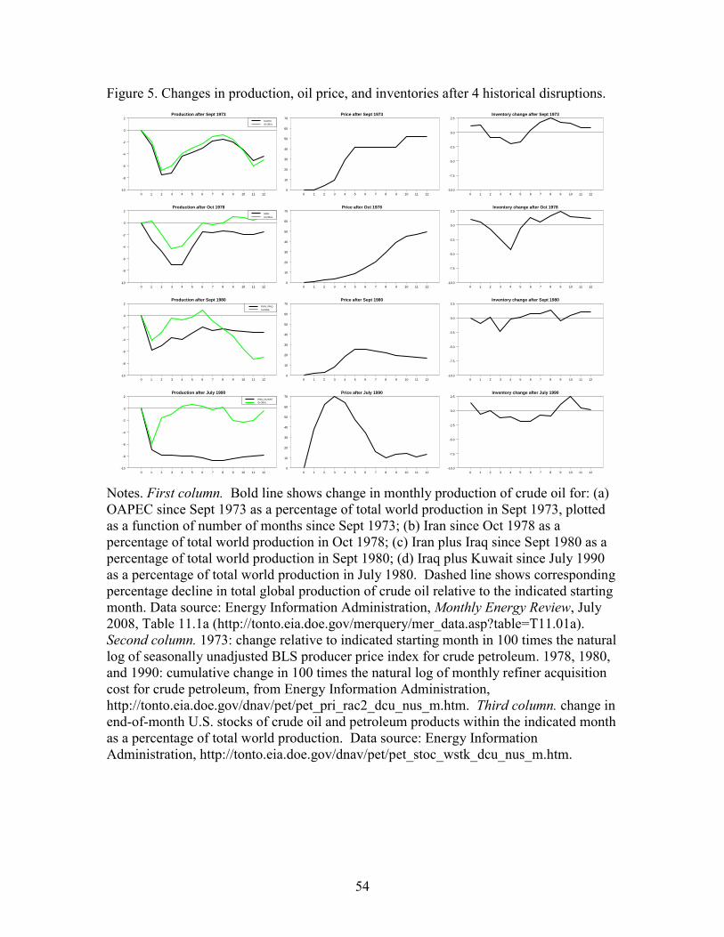
54

Figure 5. Changes in production, oil price, and inventories after 4 historical disruptions. Production after Sept 1973

0 1 2 3 4 5 6 7 8 9 10 11 12-10

-8

-6

-4

-2

0

2OAPEC

GLOBAL

Production after Oct 1978

0 1 2 3 4 5 6 7 8 9 10 11 12-10

-8

-6

-4

-2

0

2IRAN

GLOBAL

Production after Sept 1980

0 1 2 3 4 5 6 7 8 9 10 11 12-10

-8

-6

-4

-2

0

2IRAN_IRAQ

GLOBAL

Production after July 1990

0 1 2 3 4 5 6 7 8 9 10 11 12-10

-8

-6

-4

-2

0

2IRAQ_KUWAIT

GLOBAL

Price after Sept 1973

0 1 2 3 4 5 6 7 8 9 10 11 120

10

20

30

40

50

60

70

Price after Oct 1978

0 1 2 3 4 5 6 7 8 9 10 11 120

10

20

30

40

50

60

70

Price after Sept 1980

0 1 2 3 4 5 6 7 8 9 10 11 120

10

20

30

40

50

60

70

Price after July 1990

0 1 2 3 4 5 6 7 8 9 10 11 120

10

20

30

40

50

60

70

Inventory change after Sept 1973

0 1 2 3 4 5 6 7 8 9 10 11 12-10.0

-7.5

-5.0

-2.5

0.0

2.5

Inventory change after Oct 1978

0 1 2 3 4 5 6 7 8 9 10 11 12-10.0

-7.5

-5.0

-2.5

0.0

2.5

Inventory change after Sept 1980

0 1 2 3 4 5 6 7 8 9 10 11 12-10.0

-7.5

-5.0

-2.5

0.0

2.5

Inventory change after July 1990

0 1 2 3 4 5 6 7 8 9 10 11 12-10.0

-7.5

-5.0

-2.5

0.0

2.5

Notes. First column. Bold line shows change in monthly production of crude oil for: (a) OAPEC since Sept 1973 as a percentage of total world production in Sept 1973, plotted as a function of number of months since Sept 1973; (b) Iran since Oct 1978 as a percentage of total world production in Oct 1978; (c) Iran plus Iraq since Sept 1980 as a percentage of total world production in Sept 1980; (d) Iraq plus Kuwait since July 1990 as a percentage of total world production in July 1980. Dashed line shows corresponding percentage decline in total global production of crude oil relative to the indicated starting month. Data source: Energy Information Administration, Monthly Energy Review, July 2008, Table 11.1a (http://tonto.eia.doe.gov/merquery/mer_data.asp?table=T11.01a). Second column. 1973: change relative to indicated starting month in 100 times the natural log of seasonally unadjusted BLS producer price index for crude petroleum. 1978, 1980, and 1990: cumulative change in 100 times the natural log of monthly refiner acquisition cost for crude petroleum, from Energy Information Administration, http://tonto.eia.doe.gov/dnav/pet/pet_pri_rac2_dcu_nus_m.htm. Third column. change in end-of-month U.S. stocks of crude oil and petroleum products within the indicated month as a percentage of total world production. Data source: Energy Information Administration, http://tonto.eia.doe.gov/dnav/pet/pet_stoc_wstk_dcu_nus_m.htm.

55

Figure 6. Alternative measures of the size of the oil shock of 2007-08.

0

10

20

30

40

50

60

70

Aug Oct Dec Feb Apr Jun

PPIWTIRACCPIPCE

Notes. Cumulative change since August 2007 in 100 times the natural log of the indicated series. PPI = producer price index for crude petroleum. WTI = monthly average price of West Texas Intermediate. RAC = refiner’s acquisition cost for crude petroleum. CPI = consumer price index for gasoline. PCE = implicit price deflator for personal consumption expenditures on energy goods and services.

56

Figure 7. World oil production, 2003-2008.

60657075808590

2003 2004 2005 2006 2007 2008

Notes. Thin line. Monthly global crude oil production, including lease condensate, natural gas plant liquids, other liquids, and refinery processing gain, in millions of barrels per day, 2003:M1-2008:M10. Data source: Energy Information Administration, “Total Oil Supply,” January 2009, Table 1.4 (http://www.eia.doe.gov/emeu/ipsr/t14.xls). Bold line: 12-month moving average of values from thin line centered at indicated date, with end-of-sample values representing average of 6 ,..., t t sx x− + for feasible s.

57

Figure 8. Crude oil production from selected countries or fields in thousands of barrels per day.

U.S.

1920 1925 1930 1935 1940 1945 1950 1955 1960 1965 1970 1975 1980 1985 1990 1995 2000 20051000

3000

5000

7000

9000

North Sea

1973 1975 1977 1979 1981 1983 1985 1987 1989 1991 1993 1995 1997 1999 2001 2003 2005 20070

2000

4000

6000

Cantarell Mexico

1996 1997 1998 1999 2000 2001 2002 2003 2004 2005 2006 20071000

1400

1800

2200

Saudi Arabia

1973 1975 1977 1979 1981 1983 1985 1987 1989 1991 1993 1995 1997 1999 2001 2003 2005 20072000

4000

6000

8000

10000

Notes. Adapted from Figures 11, 13, and 14 in Hamilton (2009). First panel. Moving average of preceding 12 months of monthly production figures for the United States, December 1920 to February 2008, from EIA, “Crude Oil Production.” Second panel. Sum of U.K. and Norway crude oil production, monthly moving average of preceding 12 months, December 1973 to June 2007, from EIA, Table 11.1b. Third panel. Annual production from Cantarell complex in Mexico. Data for 1996 to 2006 from Pemex 2007 Statistical Yearbook. Data for 2007 from Green Car Congress (http://www.greencarcongress.com/2008/01/mexicos-cantare.html). Fourth panel. Saudi monthly production January 1973 to January 2008, from EIA, Table 11.1a.

58

Figure 9. Chinese oil consumption, 1980-2007, in thousands of barrels per day.

01,0002,0003,0004,0005,0006,0007,0008,000

1980 1985 1990 1995 2000 2005

Notes. Data source: EIA, “World Petroleum Consumption, Most Recent Annual Estimates,1980-2007,” (http://www.eia.doe.gov/emeu/international/ RecentPetroleumConsumptionBarrelsperDay.xls), December 2008.

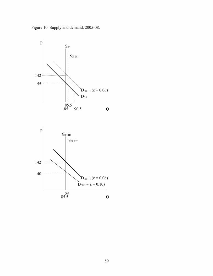
59

Figure 10. Supply and demand, 2005-08.

Q

P

85.5

40

S08:H1

86

D08:H1 (ε = 0.06)

142

S08:H2

D08:H2 (ε = 0.10)

Q

P

85

55

S05

D05

90.5

D08:H1 (ε = 0.06)

142

S08:H1

85.5

60

Figure 11. U.S. crude oil stocks: 2007, 2008, and average over 1990-2007

0

50,000

100,000

150,000

200,000

250,000

300,000

350,000

400,000

Jan Mar May Jul Sep Nov

20072008avg

Notes. Bold line: average U.S. stocks of crude petroleum (excluding Strategic Petroleum Reserve) at indicated week of year over 1990 to 2007. Data source: EIA, http://tonto.eia.doe.gov/dnav/pet/xls/pet_stoc_wstk_dcu_nus_w.xls. Thin dashed line: values for 2007. Short-dashed line: values for 2008.

61

Figure 12. Daily price of futures contracts for nearest month (1-month forward) and 3-months forward, in dollars per barrel.

0

20

40

60

80

100

120

140

160

1983 1988 1993 1998 2003 2008

near month3 months

Data source: Energy Information Administration, “NYMEX Futures Prices,” http://tonto.eia.doe.gov/dnav/pet/pet_pri_fut_s1_d.htm.

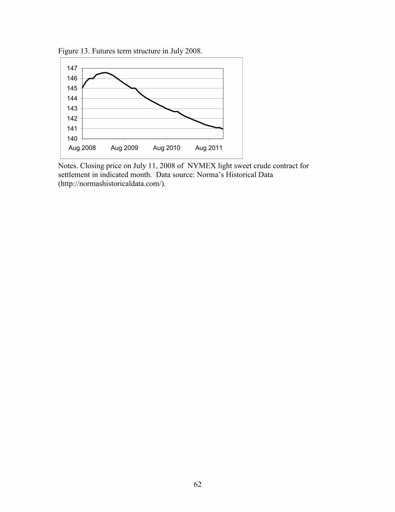
62

Figure 13. Futures term structure in July 2008.

140141142143144145146147

Aug 2008 Aug 2009 Aug 2010 Aug 2011

Notes. Closing price on July 11, 2008 of NYMEX light sweet crude contract for settlement in indicated month. Data source: Norma’s Historical Data (http://normashistoricaldata.com/).

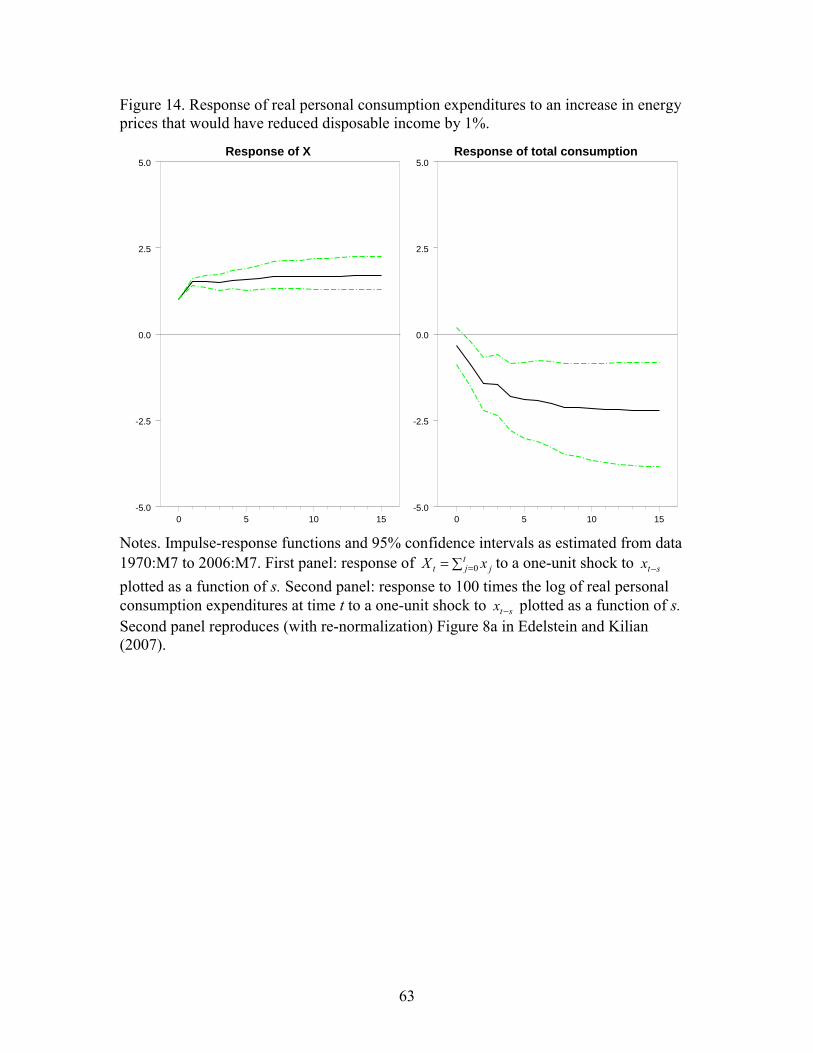
63

Figure 14. Response of real personal consumption expenditures to an increase in energy prices that would have reduced disposable income by 1%.

Response of X

0 5 10 15-5.0

-2.5

0.0

2.5

5.0Response of total consumption

0 5 10 15-5.0

-2.5

0.0

2.5

5.0

Notes. Impulse-response functions and 95% confidence intervals as estimated from data 1970:M7 to 2006:M7. First panel: response of 0

tjt jX x== ∑ to a one-unit shock to t sx −

plotted as a function of s. Second panel: response to 100 times the log of real personal consumption expenditures at time t to a one-unit shock to t sx − plotted as a function of s. Second panel reproduces (with re-normalization) Figure 8a in Edelstein and Kilian (2007).

64

Figure 15. Responses of real consumer spending on services, nondurables, and durables. Services

0 5 10 15-15.0

-12.5

-10.0

-7.5

-5.0

-2.5

0.0

2.5Nondurables

0 5 10 15-15.0

-12.5

-10.0

-7.5

-5.0

-2.5

0.0

2.5Durables

0 5 10 15-15.0

-12.5

-10.0

-7.5

-5.0

-2.5

0.0

2.5

Notes. Impulse-response functions (and 95% confidence intervals) for bivariate VARs based on energy prices and indicated component of consumption spending. Reproduces with renormalization Figure 8b-d in Edelstein and Kilian (2007).

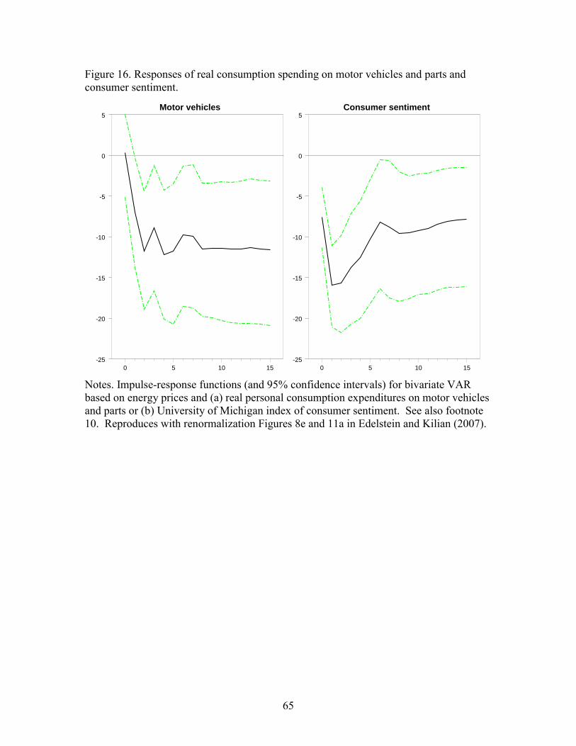
65

Figure 16. Responses of real consumption spending on motor vehicles and parts and consumer sentiment.

Motor vehicles

0 5 10 15-25

-20

-15

-10

-5

0

5Consumer sentiment

0 5 10 15-25

-20

-15

-10

-5

0

5

Notes. Impulse-response functions (and 95% confidence intervals) for bivariate VAR based on energy prices and (a) real personal consumption expenditures on motor vehicles and parts or (b) University of Michigan index of consumer sentiment. See also footnote 10. Reproduces with renormalization Figures 8e and 11a in Edelstein and Kilian (2007).

66

Figure 17. U.S. sales of domestic cars and light trucks.

U.S. domestic light truck sales(thousands of units)

0

100

200

300

400

500

600

700

800

900

1000

Jan Feb Mar Apr May Jun Jul Aug Sep Oct Nov Dec

20042005200620072008

U.S. domestic car sales

(thousands of units)

0

100

200

300

400

500

600

Jan Feb Mar Apr May Jun Jul Aug Sep Oct Nov Dec

20042005200620072008

U.S. sales of cars and light trucks manufactured in North America, in number of units sold per month. Source: http://wardsauto.com/keydata/.

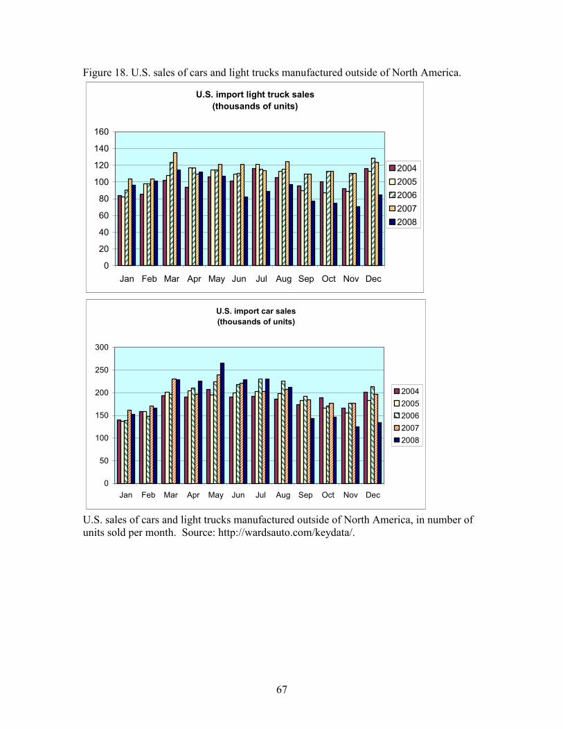
67

Figure 18. U.S. sales of cars and light trucks manufactured outside of North America.

U.S. import light truck sales(thousands of units)

0

20

40

60

80

100

120

140

160

Jan Feb Mar Apr May Jun Jul Aug Sep Oct Nov Dec

20042005200620072008

U.S. import car sales(thousands of units)

0

50

100

150

200

250

300

Jan Feb Mar Apr May Jun Jul Aug Sep Oct Nov Dec

20042005200620072008

U.S. sales of cars and light trucks manufactured outside of North America, in number of units sold per month. Source: http://wardsauto.com/keydata/.

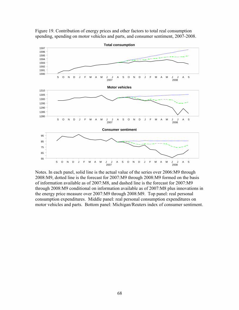
68

Figure 19. Contribution of energy prices and other factors to total real consumption spending, spending on motor vehicles and parts, and consumer sentiment, 2007-2008.

Total consumption

S O N D J F M A M J J A S O N D J F M A M J J A S2007 2008

15901591

15921593

15941595

15961597

Motor vehicles

S O N D J F M A M J J A S O N D J F M A M J J A S2007 2008

1280

1285

1290

1295

1300

1305

1310

Consumer sentiment

S O N D J F M A M J J A S O N D J F M A M J J A S2007 2008

55

65

75

85

95

Notes. In each panel, solid line is the actual value of the series over 2006:M9 through 2008:M9, dotted line is the forecast for 2007:M9 through 2008:M9 formed on the basis of information available as of 2007:M8, and dashed line is the forecast for 2007:M9 through 2008:M9 conditional on information available as of 2007:M8 plus innovations in the energy price measure over 2007:M9 through 2008:M9. Top panel: real personal consumption expenditures. Middle panel: real personal consumption expenditures on motor vehicles and parts. Bottom panel: Michigan/Reuters index of consumer sentiment.

69

Figure 20. Dynamic forecasts of GDP formed as of 2007:Q3 with and without knowledge of the ex-post values of oil prices, 2007:Q4-2008:Q4.

933934935936937938939940941942

Aug2007

Nov2007

Feb2008

May2008

Aug2008

Nov2008

predicted from AR(4)

predicted given oilpricesactual

Notes. Solid line: 100 times the natural log of real GDP. Dotted line: dynamic forecast (1- to 5-quarters ahead) based on coefficients of univariate AR(4) estimated 1949:Q2 to 2001:Q3 and applied to GDP data through 2007:Q3. Dashed line: dynamic conditional forecast (1- to 5-quarters ahead) based on coefficients reported in equation (8) (which was estimated over 1949:Q2 to 2001:Q3) applied to GDP data through 2007:Q3 and conditioning on the ex-post realizations of the net oil price increase measure #

t so + for t + s = 2007:Q4 through 2008:Q3.