Causality in Economics�

Stephen F. LeRoyUniversity of California, Santa Barbara

October 3, 2006

The initiation of quantitative analysis of formal structural models in the socialsciences is generally attributed to the Cowles Commission economists in the 1950s(see Hood and Koopmans [12] for a collection of some of the most important pa-pers). Since then the new methods have been extended and re�ned and applied inthe other social sciences. Graphical methods based on the Cowles developments areincreasingly used in the social and biological sciences. The theme of this paper isthat recent purported re�nements of the Cowles analysis, particularly as it relates torepresentations of causal relations in formal models, departed from the Cowles analy-sis to a greater extent than is commonly realized. The suggestion is that the Cowlesdevelopment as interpreted here compares favorably to more recent developments.

1 Causation

The term �structural�was given several distinct, though related, meanings by theCowles economists, as has frequently been observed. At a minimum, the term refersto the distinction between the structural form and the reduced form of a model. Inthe structural form each internal variable is expressed as a function of some otherinternal variables and some external variables, whereas the reduced form referred tothe solution of a model, in which each internal variable is expressed as a function ofthe external variables alone.As the term implies, the structural form was viewed as more fundamental than the

reduced form. It was seen as containing information not present in the reduced form,such as exclusion restrictions. For example, a structural supply-demand systemmightspecify that one or several of the external variables a¤ect demand but not supply, orvice-versa. These restrictions were used to identify structural coe¢ cients.A second meaning of �structural�, one more basic than that discussed above, has

to do with invariance under intervention. The Cowles economists implicitly dis-tinguished two classes of hypothetical experiments: (1) determining the e¤ects of

�First draft August 25, 1999. I have received helpful comments from Nancy Cartwright, DanielHausman, Damien Fennell, Julian Reiss and two referees..

1

routine realizations of external variables, and (2) analyzing changes in model struc-ture. There is no formal justi�cation for this distinction since hypothetical modelshifts can always be parametrized, allowing the analyst to represent an interventionon the structure of a model via a hypothetical shift in an external variable. Thusin a model that is structural in this sense coe¢ cients can be treated as if they wereexternal variables: an intervention on one or several model coe¢ cients by de�nitionleaves other coe¢ cients unchanged. The Cowles economists were often unclear as towhen they were treating coe¢ cients as external variables and when they were treatingthem as constants.This conception of structural models has left its tracks in current practice in

macroeconomics: the Lucas critique, with its assertion that policy change is properlymodeled as an intervention on parameters rather than variables, is one example. Thedistinction between deep and shallow parameters is another.In many analyses �structural�has a further meaning: a structural equation is

one in which the right-hand side variables are causes of the left-hand side variable.In structural equations so de�ned the equals sign has the meaning of the assignmentoperator in computer languages, as Pearl [22] observed (Pearl�s work is discussed be-low). This is distinguished from its meaning in mathematics, under which equalityby de�nition treats the right-hand side and left-hand side of an equation symmet-rically. Graphical analyses of causation have heretofore been based on this causalinterpretation of structural equations: the graphical representation of the equals signis an arrow from the right-hand side variables to the left-hand side variable.With a few exceptions, economists have been conspicuous in their absence from

these developments in recent years. It is true that the topic of causation has beenof passing interest to economists� witness Granger causality� but there is essentiallyno connection between the lines of inquiry that economists have pursued and thegraphical methods used in the other disciplines. It is clear why economists have notadopted the new graphical methods: economic models use the equality symbol withits usual mathematical meaning, not with the meaning of the assignment operator.1

Therefore economic models are not expressible as graphs, at least insofar as graphsare based on the causal interpretation of the equality symbol. That being so, econo-mists�lack of interest in graphical analyses of causation is not surprising. Further,economic models in the tradition of general equilibrium theory (including modernmacroeconomics) make no use of the structural form/reduced form distinction.These issues require more careful examination. We begin with Simon, whose

analysis of causation is in fact completely di¤erent from that implicit in the graphical

1Some contemporary studies of causation in economic models carry over the interpretation ofright-hand side variables as causes of the left-hand side variable. This is clearly so with Pearl [22].In a supply-demand model Heckman [11] justi�ed putting quantity on the left-hand side and priceon the right-hand side on the grounds that in competitive models individuals are modeled as price-takers. It is not clear to what extent Heckman�s formal analysis depends on this interpretation.Pearl and Heckman�s work is discussed below.

2

treatments. Contrary to the implication in the preceding paragraph and the pre-sumption in many expositions of graphical analysis of causation, Simon�s de�nitionof causal orderings does not require a model that is structural in the sense that theequals sign is interpreted as causal.

1.1 Notation

One problem that the reader of the literature on causation encounters is that termi-nology is sometimes not clearly de�ned and, further, many of the terms are used withdi¤erent meanings by di¤erent authors. To forestall confusion we begin by de�ningthe terminology used here. It seems to me that these de�nitions are close to standardusage, insofar as standard usage exists, but some analysts appear to disagree.2

One essential distinction, stressed in logic and mathematics but often blurred inphilosophical discourse and economic analysis, is that between variables and con-stants.3 A variable is the argument or value of a function, while a constant is astandin for a number. By specifying that � is a constant, the analyst stipulatesthat it makes no sense to consider alternative values of �� doing so makes no moresense than asking what would happen in mathematics if � took on a value other than3.14159. Variables, in turn, may be classi�ed into external and internal variables.Internal variables are determined by the model; external variables are taken as modelinputs. Therefore a model consists of a map from the space of external variablesto that of internal variables. Of course, in some exercises involving formal models,such as data-description exercises, variables are not classi�ed as between external andinternal variables, making it impossible to discuss causation.4 Since causation is thesubject here, we will assume that the analyst is willing to make this categorization.The terms �exogenous variable�and �endogenous variable�are often used with

the same meaning as �external variable�and �internal variable�, and the etymologyof the former pair of terms supports this usage. However, econometricians sometimesuse the term �exogenous variable�with a di¤erent meaning: roughly, an exogenousvariable is an observed variable of which an unobserved equation error is independentor mean-independent. Leamer [17] itemized the various meanings of �exogenous�and�endogenous� in the economics and econometrics literature. We follow his recom-mendation that the terms �external variable�and �internal variable�be substitutedto avoid confusion.It is assumed that all interventions on a model� that is, all hypothetical exper-

iments involving the model� can be characterized, either explicitly or implicitly, asinterventions on the external variables. Direct interventions on the internal variables

2For example, Hoover [15], p. 171, referred to the paper preceding this one (LeRoy [18]), which hassubstantially the same terminology, as o¤ering a �complex and di¢ cult terminological landscape�.

3As observed above, the Cowles economists were sometimes unclear as to whether model coe¢ -cients were to be interpreted as constants or external parameters.

4See Shafer [24] for an extended formal discussion of causation that dispenses almost completelywith the distinction between external and internal variables.

3

are inadmissible precisely because these variables are determined by the externalvariables. Thus hypothesized interventions on internal variables must be implic-itly attributed to interventions on the external variables that determine them. Ouranalysis of causal orderings is predicated on this characterization of interventions.It is assumed that external variables satisfy the �variation-free�condition: the

external variables can be intervened on independently. If this condition fails, theinterpretation is that there exists a functional relation linking the external variables.If so, that relation should be included in the model. The variation-free conditionasserts that the model is �invariant under intervention�, to use a phrase favored bythe Cowles economists: a hypothesized change in one external variable leaves theother external variables unchanged, and does not otherwise alter the structure of themodel.In multidate models we distinguish between parameters and processes. A para-

meter is a variable which one wants to distinguish from a constant, while a processis a collection of variables, one for each element of some index set representing time.Equivalently, one could de�ne a parameter as a process each element of which is as-sumed to take on the same value. In many discussions the terms �constant� and�variable�are used where we use �parameter�and �process�, but this usage wouldinvite confusion in the present paper because of the di¤erent de�nitions of constantand variable presented above. Parameters and processes, like variables, may beexternal or internal.Observe that in this usage the term �variable�is used in static but not dynamic

models, while the opposite is the case for the terms �parameter�and �process�. Incontrast, in much applied work involving static models the term �parameter�is usedwith the same meaning as �variable�under the above de�nition. Also, in multidatemodels the term �variable� is often used with the meaning of �process�as de�nedabove. Generally there is no harm in either of these usages, but in the present contextthey would cause confusion: in static models variables as de�ned here are the sameas parameters, so one of these terms should be deleted, while in multidate models wehave already de�ned processes as collections of variables.In some discussions the term �parameter�is used with a di¤erent meaning. For

example, Hoover [15] de�ned a parameter as a variable that is subject to direct control(p. 61). This de�nition appears to coincide with our de�nition of an external variable(or an external process). In some of Hoover�s applications parameters are assumedto take on di¤erent values at di¤erent dates, although Hoover did not time-subscriptparameters or identify them as processes, as would seem to be appropriate at leastaccording to the notation adopted here. The same practice is followed in many othersources (Engle, Hendry and Richard [4] is an example). The merits of Hoover�sterminology are not clear; however, our point here is to set out the notation of thepresent paper, not to argue against other possible choices.Variables may be either observed by the analyst, or unobserved. External un-

observed variables will be assigned probability distributions, and these will induce

4

probability distributions on internal variables, both observed and unobserved (as-suming that models have unique solutions, as we do throughout this paper). We willassume that constants are unobserved. In writing down uninterpreted models, thefollowing notation is adopted:

external observed variables or processes xinternal observed variables or processes y

unobserved constants a; b; A;B;C;D; �; �unobserved external variables or processes u

external parameters �internal parameters

(with interpreted models it is sometimes easier to depart from this notation so as touse variable names that evoke the meaning of the variable). Note that this classi�ca-tion is incomplete; other possibilities, such as internal unobserved processes (latentvariables, in some characterizations) are deleted because they are not considered inthis paper.Below we will be considering the consequences of classifying terms as constants or

coe¢ cients. Now, as a logical matter we should be specifying a name for an entity thatcould be either a variable or a constant (�term�and �entity�are unsatisfactory), andwe should also add a new symbol so as to avoid the need to write a or x. However,expanding the notation in this way is obviously unweildy. In dealing with modelsthat are linear in variables we can use the term �coe¢ cient�, so as to be able to statethat a linear model becomes bilinear if coe¢ ents are treated as variables rather thanconstants. In some contexts below we will use the term �coe¢ cient� in this senseeven when the context does not require the limitation to linear/bilinear settings. Noconfusion should result.

1.2 Simon�s De�nition

We begin with a (somewhat unconventional) review of Simon�s de�nition of causation.Suppose that a model is representable as a linear operator from Rm; a space ofexternal variables, into Rn, a space of internal variables. This operator is assumedto be representable by an n�m matrix C of constants:

y = Cx: (1)

Here (1) is the reduced form.Assume that (1) A is an n�nmatrix of constants with zeros on the main diagonal,

(2) B is an n�m matrix of constants, and (3) A and B satisfy

(I � A)�1B = C: (2)

5

Under these assumptions the model (1) can be written in the form

y = Ay +Bx; (3)

as is readily veri�ed by substituting the left-hand side of (2) for C in (1).Simon de�ned causal orderings from (3): for two internal variables y1 and y2; y1

causes y2� denoted y1 ! y2� if y1 appears in the block of equations that determiney2; and also in a block of equations of lower order (see Simon [25] for de�nitions ofthese terms). For example, in the model

y1 = b11x1 + b12x2 (4)

y2 = a21y1 + b23x3; (5)

we have y1 ! y2 because y1 appears in equation (5), which determines y2, but alsoin equation (4), which by itself constitutes a lower-order block. Formally, the causalordering on Y , the set of internal variables, associated with a given structural modelis a subset of Y � Y ; y1 ! y2 means that (y1; y2) is in the ordering.In identifying the model (4)-(5) with the causal ordering y1 ! y2 we are implicitly

assigning generic values to the coe¢ cients. In special cases (for example, in the casea21 = 0 above) y1 does not cause y2: For reference below, note that the assumptionthat the coe¢ cients are nonzero is not su¢ cient to assure the uniqueness of causalorderings; we will see that if coe¢ cients obey certain restrictions, but restrictionsthat do not involve zero values, causal orderings are altered. Since these restrictionsare nongeneric, assuming genericity assures uniqueness. This is demonstrated below.This quali�cation is not repeated below, but it is assumed.There is a well-known di¢ culty with the above account of causation: algebraic

operations on the equations of (3) can apparently alter causal orderings. For example,substituting (4) in (5) results in

y2 = a21b11x1 + a21b12x2 + b23x3: (6)

In the model (4), (6) neither y1 nor y2 causes the other according to Simon�s de�nition.Di¤erent algebraic operations result in models in which y1 and y2 are simultaneouslydetermined, or obey y2 ! y1, even though each of these models represents the samelinear operator C. It appears as if apparently innocuous mathematical operationsalter causal orderings.This problem re�ects the fact that the matrices A and B associated with a given

C by (2) are not unique. Therefore on Simon�s de�nition the causal ordering of theinternal variables depends on which of an in�nite number of pairs of matrices A andB satisfying (2) is chosen.To avoid the problem posed by the apparent dependence of causal orderings on

algebraic operations, we impose a further restriction: we require that each equationcontain at least one external variable not found in any other equation. Hereafter

6

we refer to this condition as the exclusion condition.5 The exclusion condition rulesout algebraic operations that involve more than one equation (because if the originalmodel satis�es the exclusion condition, the modi�ed model will not). For example,the model (4), (6) does not satisfy the exclusion condition: the external variablesthat appear in (4)� x1 and x2� also appear in (6).Satisfaction of the exclusion condition requires that C have rank n. If the exclusion

condition is satis�ed and if in addition the model has the same number of internalas external variables, then causal orderings are unique. To see this, note that underthe assumed condition C is nonsingular, so (1) can be solved to yield

x = C�1y: (7)

If D is de�ned by D = I � C�1, where I is the identity matrix, this becomes

y = Dy + x: (8)

Since D is unique in (8), it is clear that the causal ordering is unique.If m � n, with any C there is always associated at least one pair A and B that

satis�es the exclusion condition: the fact that C is of rank n implies that one canalways �nd a square nonsingular matrix C1 and a matrix C2 such that the externalvariables x can be partitioned (perhaps after reordering) into (x1; x2) and (1) can bewritten in the form

y = C1x1 + C2x2: (9)

Premultiplying by C�11 results in

C�11 y = x1 + C�11 C2x2: (10)

As before, if D is de�ned by D = I � C�11 ; (10) can be written as

y = Dy + x1 + C�11 C2x2: (11)

Here each x1 enters one and only one of the equations. The variables in x2 can enterin any or all of the equations.Damien J. Fennell [5] pointed out that if m > n; causal orderings under Simon�s

de�nition are not unique even if the exclusion condition is imposed. This is sobecause with m > n; di¤erent subsets of the external variables can be selected tosatisfy the exclusion condition, and each choice implies a di¤erent causal ordering.To see this, consider the system

y1 = b11x1 + b12x2 (12)

y2 = b22x2 + b23x3; (13)

5The exclusion condition is essentially the same as Hausman�s independence condition ([9], p.64). See also Hoover [14], p. 103 ¤.

7

in which y1 and y2 are not causally ordered: The exclusion condition is satis�ed bythe presence of x1 in (12) and x3 in (13). However, if (13) is solved for x2 and theresult is substituted in (12), we obtain

y1 = b11x1 + a12y2 � (b12b23=b22)x3: (14)

y2 = b22x2 + b23x3; (15)

where

a12 = b12=b22: (16)

In the system (14)-(15) the exclusion condition is again satis�ed because of the ex-clusion of x2 in (14) and x1 in (15). In (14)-(15) we have y2 ! y1. Since (12)-(13)is mathematically equivalent to (14)-(15), it follows that causal orderings are notunique.Despite this, causal orderings are unique generically: in (14)-(15) we have y2 ! y1,

but that version of the model is nongeneric because of the restriction (16). Since wehave already ruled out nongeneric special cases, it is seen that Fennell�s observationabout nonuniqueness of causal orderings when m > n does not involve anything new.It is noteworthy that assuming that a model satis�es the exclusion condition is

weaker than assuming that it is structural in the sense that the equality symbol isasymmetric: imposition of the exclusion condition allows renormalization of indi-vidual equations (i.e., expressing them so that a di¤erent variable appears on theleft-hand side), so it does not matter which variable is located on the left-hand side.Causal orderings as Simon de�ned them are not altered by such renormalizations. Incontrast, under the causality de�nition based on the asymmetric interpretation of theequality symbol, renormalizations of individual equations result in a di¤erent modelwith a di¤erent causal ordering. That Simon�s de�nition of causation does not relyon an unconventional interpretation of the equality symbol is an attractive feature ofhis treatment.The foregoing discussion is very close to Simon�s development. On a super�cial

comparison of the above discussion with Simon�s paper, it appears that the exclusioncondition has nothing to do with Simon�s Section 6 discussion of when causal struc-tures are �operationally meaningful�. In fact, however, Simon�s discussion is entirelyconsistent with the discussion here; the apparent di¤erences are terminological.

Simon�s Section 6 marks a change from the discussion that preceded it in hispaper. Prior to that section Simon did not explicitly incorporate external variablesin his discussion (except in Example 4.2), as that term is used here. His examplescontained only variables x and constants a (or �). Simon�s x corresponds to our y;his a (or �) corresponds to our x and a. Simon used the terms �exogenous variable�and �endogenous variable�, but he assigned them a meaning that is derived fromhis de�nition of causal orderings: on Simon�s usage if we have y1 ! y2, then y1 is

8

exogenous in the set of equations that determine y2, and y2 is endogenous in thatset.However, in Section 6 in dealing with the fact that algebraic operations can appar-

ently alter causal orderings, Simon considered interventions in the a terms, implyingthat in that section he was viewing the a terms as variables that are external in thesense of this paper, as opposed to constants as in the earlier sections.Simon did not distinguish between the coe¢ cients and the intercept terms, im-

plying that he was allowing for interventions in either. Here, in contrast, we are sim-plifying relative to Simon by maintaining the assumption that the coe¢ cient termsare constants, so that they are not subject to intervention, implying that only the in-tercept terms are treated as external variables. Treating the coe¢ cients as variableswould convert what is a linear model into a bilinear model. Following Simon herewould complicate the discussion unnecessarily (a bilinear model is considered brie�yin Sec. 1.5).For Simon, causal orderings are operationally meaningful only if the equations of

a structural model have �individual identities�. The equations of a structural modelhave �individual identities�insofar as interventions can be associated with particularequations or subsets of equations. In the terminology of the present paper, theseinterventions are associated with external variables. Therefore, translating into theterminology of the present paper, Simon�s criterion for operational meaningfulnessis that particular external variables be associated with particular equations. Thiscorresponds exactly to our exclusion condition.Simon stated this explicitly: �The causal relationships have operational meaning,

then, to the extent that particular alterations or �interventions�in the structure canbe associated with speci�c complete subsets of equations� (p. 65). Continuing,�[w]e found that we could provide [a causal] ordering with an operational basis if wecould associate with each equation of a structure a speci�c power of intervention, or�direct control.� ... Hence, ... structural equations are equations that correspond tospeci�ed possibilities of intervention�(p. 66).Simon�s discussion would have been clearer if he had explicitly incorporated this

idea in his de�nition of causal orderings, as we have, rather than implicitly attachingthe relevant condition later as a condition for causal orderings to be operationallymeaningful. This is, of course, a criticism of exposition, not substance.Our simpli�cation (relative to Simon) of treating coe¢ cients as constants rather

than external variables does not alter the substance of Simon�s argument: it is easyto see from examination of examples that if y1 ! y2 when the coe¢ cients are treatedas constants, the same is true when the coe¢ cients are treated as external variables.6

Assuming that the model is linear in variables (a consequence of treating the coe¢ -cients in Simon�s model as constants) limits the direct applicability of the analysis;contemporary models are likely to be nonlinear. Again, however, the analysis can

6However, the converse is not true: changing an external variable to a constant reduces the setof possible interventions, implying that y1 may no longer cause y2.

9

be extended to the general case. The principal di¤erence between the analysis ofcausation in linear vs. nonlinear models is that in the latter case causal orderingsare no longer associated with constants measuring the strength of causal e¤ects: ingeneral the magnitude of a given change in the cause variable on the e¤ect variabledepends on the values of all external variables.The theme of this paper is that Simon�s analysis of causation di¤ers in major

respects from more recent treatments. At this stage we point out some of thedistinguishing features of Simon�s treatment. First, Simon made clear that he wasanalyzing causation in the context of a formal model, not causation as it appliesdirectly to reality or perceived reality. In contrast, in virtually all discussions in thephilosophy literature, and in some in the economics literature, causation is discussedas a direct feature of reality. Second, under Simon�s de�nition causality is not amatter of how a model is interpreted or applied: rather, the causal ordering impliedby a model can be inferred unambiguously from its formal structure. Third, underSimon�s treatment models are written in the usual form as maps from external tointernal variables. As noted above, under some alternative treatments of causationthe equals sign is interpreted as asymmetric, with cause variables on the right-handside and e¤ect variables on the left-hand side. In all three respects we follow Simon�slead in this paper.These features of Simon�s treatment of causality have the implication that some

sentences that are customarily interpreted as causal do not satisfy the formal re-quirements for causation. For example, consider the statement �I drank too muchyesterday (D); as a result I fell asleep while smoking (S), and my doing so caused myhome to burn down (B)�. Here D is clearly external, and it would be natural to di-agram this sentence as �D ! S ! B�. The problem is that the exclusion conditionfor �S ! B�fails: there does not exist an external variable that a¤ects B but notS: Equivalently, S is determined in the same block of equations as B; implying thatS and B are appropriately treated as simultaneous, not causally ordered. It followsthat the inference that S caused B is a feature of the interpretation of the model,not its formal structure.The fact that sometimes we are willing to infer causation in settings where Si-

mon�s formal analysis does not justify this inference does not re�ect any shortcomingin Simon�s treatment. Informal statements of causation, such as that just given, gen-erally presume unstated background conditions (�the �re extinguisher did not work(E), so I could not put out the �re�). Explicit incorporation of variables represent-ing background conditions generally allows satisfaction of the exclusion condition fora causal ordering. In this case E would be included as an external variable thatappears in the external set of B but not that of S: Under this modi�cation we wouldhave S ! B7.

7In this example causality is expressed as a relation among events rather than variables. Thereader can supply the indicated modi�cation of the formal structure set out above so as to deal withthis case.

10

1.3 Causality as Su¢ ciency8

Part of the reason Simon�s characterization of causation is not much used currentlyis that Simon did not provide a clear explanation of what follows if one variablecauses another. What does the fact that the cause variable is determined in a lower-order subsystem relative to the e¤ect variable have to do with causation? What isthe content of �operationally meaningful�in this context, and what is the connectionbetween this concept and the exclusion condition? What interventions are admissibleif y1 causes y2, but not otherwise? What is the interpretation of these interventions?The best way to supply intuitive content to causation is to consider simple ex-

amples. We will see that in some cases it is clear that causal statements are notappropriate, while in other cases it is equally clear that they are. Examination of thedi¤erence between these examples will suggest the general principle. This principleis stated more formally in the next subsection.Consider the supply-demand model

qs = aspp+ bsww (17)

qd = adpp+ bdii (18)

qs = qd = q; (19)

where qs is quantity supplied, qd is quantity demanded, q is equilibrium quantity, i isincome, p is price and w is weather. Here weather and income are external and theother variables are internal.In the system (17)-(19) the question �What is the e¤ect of weather on the equilib-

rium quantity?�is unambiguous: the e¤ect can be directly calculated from the model.This is so because weather is external. However, if one were to ask �What is thee¤ect of price on equilibrium quantity?�the appropriate response would be that thequestion is misposed. Price and quantity are both internal; they are simultaneouslydetermined, and neither is causally prior to the other.The reasoning here is worth elaborating. The assumed intervention results in

the price changing from, say, p to p +�p: The problem is to infer the e¤ect of thisintervention on q. The reason the question is ambiguous is that any of an in�nitenumber of pairs of shifts in the external variables �weather� and �income� couldhave caused the assumed change in price, and these interventions map onto di¤erentvalues of q. Thus the reason the question is misposed is that it does not give enoughinformation about the intervention being considered to allow a unique answer.The suggestion is that causal statements involving internal variables as causes are

ambiguous, and therefore inadmissible, except when all the interventions consistentwith a given change in the cause variable map onto the same change in the e¤ectvariable. One is led to de�ne two internal variables as causally ordered when theindicated condition is satis�ed, and not otherwise.

8The material presented in this and the following subsections is drawn from LeRoy [18].

11

Now consider the model

qs = bsww + bsff (20)

qd = adpp+ bdii (21)

qs = qd = q; (22)

where f is fertilizer. Weather, fertilizer and income are the external variables. Hereeven though q is internal there is no problem with the assertion that q causes p:This is so because all the interventions in weather and fertilizer consistent with agiven change in q map onto the same value of p, as the structure of the model makesobvious.

1.4 A Formal Statement

Let the external set Xj for a particular internal variable yj be the minimal set ofexternal variables such that yj can be written as a function of Xj. Then the model(1) can be written in the form

yj = �jXj j = 1; :::; n; (23)

where Xj is a vector of which the elements are the members of Xj; and �j is aconformable vector of constants. Of course, �j coincides with the j-th row of C withthe zero elements deleted.Suppose that Xi �� Xj, where �� means �is a proper subset of�. Hereafter we

will call this the subset condition. Further, de�ne Xj;i as Xj � Xi (i.e., as the setconsisting of the elements of Xj that are not in Xi). De�ne Xj;i as a vector of whichthe elements are the members of Xj;i. Suppose in addition that there exists a scalarconstant j;i and a vector of constants �j;i such that (23) can be written in the form

yj = �jXj = j;iyi + �j;iXj;i: (24)

Existence of j;i and �j;i with this property implies that all the interventions in Xi

consistent with a given change in yi have the same e¤ect on yj: Thus all the in-formation relevant for yj contained in Xi is summarized in yi, so that even thoughmany possible interventions in Xi could have caused the variation in yi, each possi-ble intervention has the same e¤ect on yj: When j;i and �j;i exist that satisfy theabove property we will say that yi is a simple cause of yj, and will write yi ) yj:Thus yi ) yj means that yi is su¢ cient for Xi in the determination of yj. We willcall the condition that there exist j;i and �j;i with the properties just described thesu¢ ciency condition. Thus we have yi ) yj if and only if both the subset conditionand the su¢ ciency condition are satis�ed.In general, Xi �� Xj does not imply existence of j;i and �j;i satisfying (24).

Therefore it will not generally be the case that Xi �� Xj implies yi ) yj. However,

12

if Xi �� Xj, there may exist some other internal variable yk that satis�es the subsetcondition such that all the interventions in Xi consistent with a given change in yiand a given value of yk map onto the same value of yj: Then we have conditionalcausation, indicated by yi ) yjjyk: Still more generally, the conditioning set mayinclude several internal variables rather than just one, and may include one or moreof the external variables.Two conditions are required for conditional causation. First, yi must be variation-

free: if the variables held constant completely determine yi, it makes no sense totalk about the e¤ect of variations in yi on yj, ceteris paribus. For example, if theconditioning set includes all the external variables, no variation in yi is possible. Moreprecisely, the variation-free condition is satis�ed for yi ) yjjyk if the model permitsindependent variation in yi and yk without restricting yjSecond, if we are to have yi ) yjjyk; the conditioning set must be such as to

ensure that all values of the external variables Xi consistent with a given change inyi and a given level of yk produce the same change in yj: This requirement, whichcorresponds to the su¢ ciency requirement for simple causation, is needed to avoidambiguity in the e¤ect of variations in the external set for yi on yj:As long as Xi �� Xj, there will always exist some subset (possibly the null set,

if yi ) yj) of the external and internal variables such that yi causes yj conditionalon that set of variables. We will write yi ! yj if either yi ) yj or yi ) yjjzk forsome scalar or vector zk. Thus yi ! yj under the de�nition just given is equivalentto Xi �� Xj:If yi ! yj, there exists a set of conditioning variables zk such that yi ) yjjzk, but

that set is not necessarily unique. For example, in the model

y1 = b11x1 + x2 (25)

y2 = a21y1 + b21x1 + x3; (26)

where x1; x2 and x3 are external variables, we have y1 ) y2jx1, but also y1 ) y2jx2:In the �rst case the intervention is on x2, while in the second case it is on x1: Thecoe¢ cient associated with y1 ) y2jx1 is clearly a21: However, in the case of y1 ) y2jx2matters are more complicated: we must distinguish between the direct e¤ect of x1 ony2, which has coe¢ cient b21; and its indirect e¤ect. The indirect e¤ect has coe¢ cienta21 if the cause variable is identi�ed with y1, and a21b11 if it is identi�ed with x1:Conditional causation may raise problems of interpretation. The indicated inter-

vention requires a nonzero change in the variables in Xi; with the changes requiredto satisfy a linear relation so as to hold yk constant. Existence of such functionalrelations among external variables appears to con�ict with the assumption that theexternal variables are variation-free. If there exists a functional relation among thevariables in Xi, then assuming that these variables are external is a misspeci�cation.Thus the intervention is inappropriate to the assumed model.

13

In other cases this problem does not arise. For example, in the important casewhen the matrix A in the model (3) is triangular (not just block-triangular), eachyi causes yj (i < j) conditional on y1; y2; :::yi�1; yi+1; :::yj�1: However, the indi-cated intervention involves only one external variable, so there is no violation of thevariation-free condition.It is easily veri�ed that the above de�nition of yi ! yj coincides with Simon�s

de�nition: assuming that the exclusion condition is satis�ed, yi appears in the blockof equations that determines yj and also in a lower-order block if and only if Xi ��Xj. Thus yi ! yj can refer to both conditional causation as de�ned here and Simon�sde�nition of causation.

1.5 Causality and Parameter Interventions

Up to now we have taken coe¢ cients to be constants rather than variables or pa-rameters. This assumption was for convenience only. Many problems involvingcausation do not satisfy this restriction. For example, as soon as coe¢ cients aretreated as external variables rather than constants, models become bilinear ratherthan linear. In this subsection we make some observations about the consequencesof treating coe¢ cients as parameters in multidate models.Neoclassical macroeconomists stress that analysis of macroeconomic policy changes

requires identifying and estimating �deep parameters� (labeled here external para-meters). This is correct if one is considering changes in policy regimes, and if one ismodeling regime change by parameter interventions, as recommended by the Lucascritique (Lucas [20]), at least on some readings. I have argued elsewhere (LeRoy [19])that whether policy changes in dynamic models are appropriately modeled throughinterventions on external parameters or on external processes depends on the ques-tion being asked: if the intervention is intended to apply to the past as well as thepresent and future, parameter interventions are indicated. If only the present and/orfuture is to be a¤ected, process interventions are indicated.An important point is that if regime changes are modeled using process rather

than parameter interventions, there is no need to model the dependence of internalparameters on external parameters. To see this, suppose that we have a model that islinear in variables if the coe¢ cients are treated as constants. As observed above, if y1tcauses y2t in this setting, then the same remains true when the coe¢ cients are treatedas parameters. This is so regardless of the causal ordering among parameters. Theonly di¤erence between the two cases is that in the latter case the external parameters,or some subset of them, are included in the exogenous sets, but this change will notcause failure of the subset and su¢ ciency conditions, assuming that these are satis�edwhen coe¢ cients are treated as constants. This point underscores the importanceof Marschak�s [21] observation that analysis of causation does not always require acomplete characterization of a model�s causal ordering.Hoover [13] pointed out that a potentially testable implication of causation is that

14

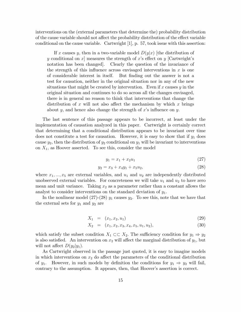
interventions on the (external parameters that determine the) probability distributionof the cause variable should not a¤ect the probability distribution of the e¤ect variableconditional on the cause variable. Cartwright [1], p. 57, took issue with this assertion:

If x causes y, then in a two-variable model D(yjx) [the distribution ofy conditional on x] measures the strength of x�s e¤ect on y [Cartwright�snotation has been changed]. Clearly the question of the invariance ofthe strength of this in�uence across envisaged interventions in x is oneof considerable interest in itself. But �nding out the answer is not atest for causation, neither in the original situation nor in any of the newsituations that might be created by intervention. Even if x causes y in theoriginal situation and continues to do so across all the changes envisaged,there is in general no reason to think that interventions that change thedistribution of x will not also a¤ect the mechanism by which x bringsabout y, and hence also change the strength of x�s in�uence on y:

The last sentence of this passage appears to be incorrect, at least under theimplementation of causation analyzed in this paper. Cartwright is certainly correctthat determining that a conditional distribution appears to be invariant over timedoes not constitute a test for causation. However, it is easy to show that if y1 doescause y2, then the distribution of y2 conditional on y1 will be invariant to interventionson X1; as Hoover asserted. To see this, consider the model

y1 = x1 + x2u1 (27)

y2 = x3 + x4y1 + x5u2; (28)

where x1; :::; x5 are external variables, and u1 and u2 are independently distributedunobserved external variables. For concreteness we will take u1 and u2 to have zeromean and unit variance. Taking x2 as a parameter rather than a constant allows theanalyst to consider interventions on the standard deviation of y1.In the nonlinear model (27)-(28) y1 causes y2: To see this, note that we have that

the external sets for y1 and y2 are

X1 = (x1; x2; u1) (29)

X2 = (x1; x2; x3; x4; x5; u1; u2); (30)

which satisfy the subset condition X1 �� X2: The su¢ ciency condition for y1 ) y2is also satis�ed. An intervention on x2 will a¤ect the marginal distribution of y1, butwill not a¤ect D(y2jy1):As Cartwright observed in the passage just quoted, it is easy to imagine models

in which interventions on x2 do a¤ect the parameters of the conditional distributionof y1. However, in such models by de�nition the conditions for y1 ) y2 will fail,contrary to the assumption. It appears, then, that Hoover�s assertion is correct.

15

2 Causality and Identi�cation

2.1 Identi�cation and Exclusion Restrictions

We have seen that exclusion restrictions play a central role in determining causalorderings. As is well known, they also play a central role in determining whether theparameters in a model are identi�ed (Fisher [7]). Despite the common role of exclu-sion restrictions in determining causality and identi�cation, the two are very di¤erentnotions. Causation is an ordering on internal variables, whereas identi�cation hasto do with whether the econometrician can make inferences about parameter valuesfrom the (population) distribution of observed variables. Causation can be de�nedand analyzed without even specifying which variables are observed, and in fact thisis exactly what we have done up to now. However, empirical estimation of causalparameters requires assumptions that assure identi�cation, and this is di¤erent fromcausation. Whether parameters are identi�ed depends not just on which variablesare excludable from which equations, but also on which variables are observed andwhat distributional assumptions are imposed on those (external) variables that arenot observed.As just noted, discussion of identi�ability requires specifying which variables are

observed by the econometrician and which are not. Both internal and externalvariables can be either observed or unobserved. Probability distributions are assignedto unobserved external variables as part of model speci�cation, and these inducedistributions on both observed and unobserved internal variables. Henceforth wewill use u to denote unobserved variables, and all other letters to denote observedvariables.To illustrate the di¤erence between causality and identi�ability, consider the

supply-demand model

q = a1p+ b1x1 + b2x2 + u1 (31)

q = a2p+ b3x1 + b4x2 + u2; (32)

where x1 and x2 are external observed shift variables (weather, income and fertilizerplayed this role above) and a1; a2; b1 and b2 are constants. As it stands, none of thecoe¢ cients in this model are identi�ed: observations on p; q, x1 and x2 cannot beused to estimate the coe¢ cients. Under the restriction b2 = b3 = 0; all coe¢ cients areidenti�ed, including a1 and a2; the price elasticities of demand and supply. However,these coe¢ cients do not measure the strength of causal relations because p is notcausally prior to q: We see that in general identi�cation is an issue in estimating notjust constants associated with causation, but also those associated with simultaneousdetermination of internal variables.In bringing empirical evidence to bear on evaluating the causal relation (or lack

thereof) between variables yi and yj in a given model, then, two questions must be

16

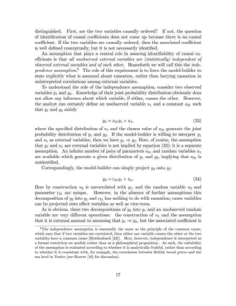
distinguished. First, are the two variables causally ordered? If not, the questionof identi�cation of causal coe¢ cients does not come up because there is no causalcoe¢ cient. If the two variables are causally ordered, then the associated coe¢ cientis well de�ned conceptually, but it is not necessarily identi�ed.An assumption that plays a central role in assuring identi�ability of causal co-

e¢ cients is that all unobserved external variables are (statistically) independent ofobserved external variables and of each other. Henceforth we will call this the inde-pendence assumption.9 The role of this requirement is to force the model-builder tostate explicitly what is assumed about causation, rather than burying causation inuninterpreted correlations among external variables.To understand the role of the independence assumption, consider two observed

variables y1 and y2. Knowledge of their joint probability distribution obviously doesnot allow any inference about which variable, if either, causes the other. However,the analyst can certainly de�ne an unobserved variable u1 and a constant a21 suchthat y1 and y2 satisfy

y2 = a21y1 + u1; (33)

where the speci�ed distribution of u1 and the chosen value of a21 generate the jointprobability distribution of y1 and y2: If the model-builder is willing to interpret y1and u1 as external variables, then we have y1 ) y2: Here, of course, the assumptionthat y1 and u1 are external variables is not implied by equation (33); it is a separateassumption. An in�nite number of pairs of parameters a21 and random variables u1are available which generate a given distribution of y1 and y2; implying that a21 isunidenti�ed.Correspondingly, the model-builder can simply project y2 onto y1:

y2 = c21y1 + u2: (34)

Here by construction u2 is uncorrelated with y1; and the random variable u2 andparameter c21 are unique. However, in the absence of further assumptions thisdecomposition of y2 into y1 and c21 has nothing to do with causation; cause variablescan be projected onto e¤ect variables as well as vice-versa.As is obvious, these two decompositions of y2 into y1 and an unobserved random

variable are very di¤erent operations: the construction of u1 and the assumptionthat it is external amount to assuming that y1 ) y2; but the associated coe¢ cient is

9The independence assumption is essentially the same as the principle of the common cause,which says that if two variables are correlated, then either one variable causes the other or the twovariables have a common cause (Reichenbach [23]). Here, however, independence is interpreted asa formal restriction on models rather than as a philosophical proposition. As such, the suitabilityof the assumption is evaluated according to whether it is analytically fruitful, rather than accordingto whether it is consistent with, for example, the correlation between British bread prices and thesea level in Venice (see Hoover [16] for discussion).

17

unidenti�ed. In contrast, the construction of u2 guarantees its uncorrelatedness withy1, but has nothing to do with causation. If we are willing to assume further thatu1 = u2� or, equivalently, that y1 and u1 are uncorrelated, or that u2 is external� wecan interpret the coe¢ cient c21 of the projection of y2 on y1 as a causal coe¢ cient.One implication of the independence assumption is that if one variable causes

another, the two variables are necessarily correlated.10 In some settings this mayseem counterintuitive. Suppose that y1t is generated according to

y1t = �11y1;t�1 + �12y2t + ut; (35)

where y2t is a regulator, the behavior of which is generated by

y2t = �21y1;t�1: (36)

Then the behavior of y1t follows

y1t = (�11 + �12�21)y1;t�1 + ut; (37)

where the external variables are ut; ut�1; :::: and y0: The de�nitions of causationimply that we have y1;t�1 ) y1t under the (heretofore unstated) assumption that�11 + �12�21 6= 0:However, suppose that the regulator is operated by choosing c so as to minimize

the unconditional variance of yt: This results in �11 + �12�21 = 0 or, equivalently,�21 = ��11=�12; implying that (37) becomes

y1t = ut: (38)

In this special case the regulator y2t is no longer correlated with y1t, and we no longerhave causation: y1;t�1 ; y1t: This result may seem to run counter to the ordinary-language usage of the term �causality�, but it is an unavoidable consequence of thede�nitions.Under any particular parametrization of a model, imposing the independence

requirement is obviously very restrictive. However, imposing independence on somerelated parametrization of the model amounts only to requiring the modeler to stateexplicitly what he is or is not willing to assume about causation. This is not anunreasonable requirement insofar as the goal is to arrive at causal conclusions. Forexample, the modeler who is willing to assume y2 ) y1 instead of y1 ) y2 wouldgenerate y1 from y1 = a12y2 + u3; with y2 and u3 assumed external and independent.Finally, if the model-builder were unwilling to assume that either y1 or y2 causes theother, he could specify the parametrization

10Of course, the converse is not true: if the external sets for two internal variables have a nonemptyintersection, the independence assumption implies that two variables will be correlated. However,if neither external set is a subset of the other, then the two variables are not causally ordered, eitherunconditionally or conditionally.

18

y1 = a12y2 + u1 (39)

y2 = a21y1 + u2: (40)

Here u1 and u2 are independent by the independence assumption, but this impliesneither y1 ) y2 nor y2 ) y1.

2.2 Causation and Regression

In LeRoy [18] it was pointed out that, under the condition that all unobserved externalvariables are independently distributed, coe¢ cients associated with causation can beestimated consistently by ordinary least squares. This is so because under the statedrestriction variables representing causes are statistically independent of error terms.It follows that econometric theory can sometimes be used to determine causation:knowledge that ordinary least squares results in inconsistency implies absence of(simple) causation. The example given to illustrate this point was the model

yt = �1yt�1 + u1t (41)

u1t = �2u1;t�1 + u2t; (42)

where the unobserved external variables u2t; u2;t�1; :::; u21; u20 and y0 are assumed tobe independent. When �2 6= 0 we have that yt�1 is correlated with u1t; so a least-squares regression of yt on yt�1 will not produce a consistent estimate of �1: From thestated result it follows that yt�1 ; yt: Checking, the subset condition for yt�1 ) yt issatis�ed, but the su¢ ciency condition fails: the elements of the external set for yt�1(these are u2;t�1; :::; u20; y0) a¤ect yt through u1t as well as through yt�1: Thereforewe have yt�1 ; yt:In response to this, Hoover [14] observed that applying the Koyck transformation

results in

yt = (�1 + �2)yt�1 � �1�2yt�2 + u2t; (43)

in which the parameters �+ � and �� are in fact estimated consistently by ordinaryleast squares. Further, separate consistent estimates of �1 and �2 are easily calculatedfrom the estimated regression coe¢ cients. Hoover appeared to view this result asraising questions about the validity of the inference that failure of ordinary leastsquares implies nonexistence of causation, although he did not point out an error inthe reasoning or spell out the argument. In fact, the multiple regression of yt onyt�1 and yt�2 is di¤erent from the univariate regression of yt on yt�1: The fact thatordinary least squares is valid in (43) suggests11 that even though we do not have the

11We use �suggests�rather than �implies�because the converse of the above result� that consis-tency of ordinary least squares implies causation� is not generally true.

19

simple causation yt�1 ) yt, we might have the conditional causation yt�1 ) ytjyt�2;and it can be directly veri�ed from the de�nition of conditional causation that thisis the case.

3 Alternative Treatments of Causality

As noted in the introduction, many expositions of contemporary macroeconometricpractice as it relates to causation give the impression that it is essentially a re�nementand extension of the Cowles insights, particularly those of Simon. The essentials,we are told, were taken over as a whole; subsequent developments added precisionand ampli�ed details, but did not a¤ect the substance. On the contrary, contempo-rary discussions are much sketchier than the Cowles treatment (although the Cowleseconomists are not beyond criticism in this respect), and they generally di¤er in es-sential respects from the Cowles treatment. The reader who is persuaded by thisassessment will be motivated to understand the di¤erences in the various treatmentsso as to determine which line o¤ers the best prospect for improving analytical prac-tice. It will shortly be clear that the view here is that to the (considerable) extentthat modern practice di¤ers from the Cowles analysis, the di¤erences do not representclear improvements.

3.1 Sims-Granger

The Cowles Commission economists emphasized that in the absence of other iden-tifying information, causal orderings are not empirically testable: two models withdi¤erent causal orderings may be observationally equivalent (it remains true that, inconjunction with other restrictions, causal orderings may be overidentifying, hencetestable). Subsequently various economists have challenged this dictum, apparentlyasserting that causation is directly testable. For example, Sims [26], p. 24, wrote:

When, as econometricians estimating models ordinarily do, someoneasserts that a particular variable or group of variables is strictly exogenousin a certain regression, that assertion is, in time series models, testable.�Exogeneity�here is given its standard econometrics textbook de�nition.Exogeneity tests are thus an easily applied test for speci�cation error, pow-erful against the alternative that simultaneous-equations bias is present.The usefulness of these speci�cation tests ought not to be controversial....

Despite the claim here that the term �exogeneity�has a standard meaning andthe presumption in this literature that this meaning is closely related to that ofcausation, de�nitional issues come to the forefront. A process y2 Granger-causesanother process y1 if lagged values of y2 predict y1 conditional on lagged values of y1:If y2 fails to Granger-cause y1 then, according to Granger [8], correlations between the

20

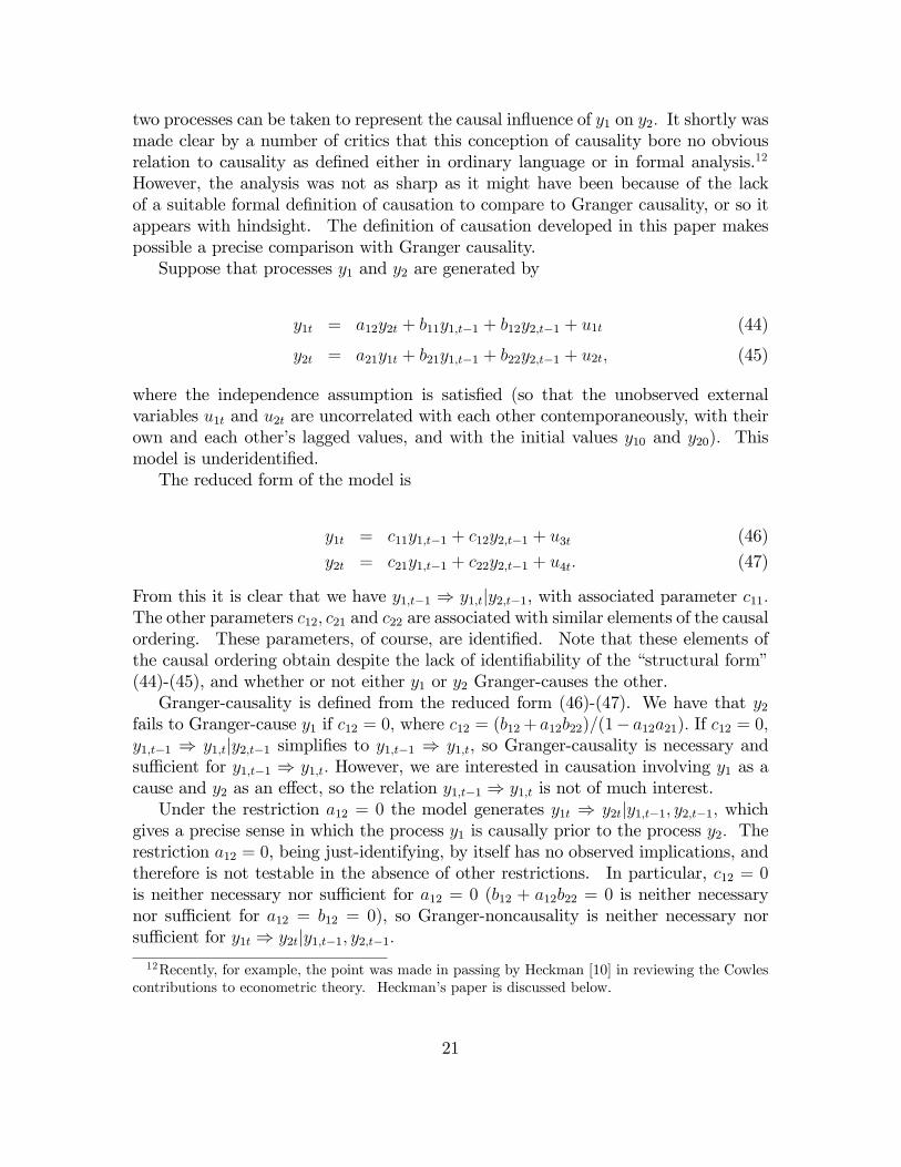
two processes can be taken to represent the causal in�uence of y1 on y2: It shortly wasmade clear by a number of critics that this conception of causality bore no obviousrelation to causality as de�ned either in ordinary language or in formal analysis.12

However, the analysis was not as sharp as it might have been because of the lackof a suitable formal de�nition of causation to compare to Granger causality, or so itappears with hindsight. The de�nition of causation developed in this paper makespossible a precise comparison with Granger causality.Suppose that processes y1 and y2 are generated by

y1t = a12y2t + b11y1;t�1 + b12y2;t�1 + u1t (44)

y2t = a21y1t + b21y1;t�1 + b22y2;t�1 + u2t; (45)

where the independence assumption is satis�ed (so that the unobserved externalvariables u1t and u2t are uncorrelated with each other contemporaneously, with theirown and each other�s lagged values, and with the initial values y10 and y20): Thismodel is underidenti�ed.The reduced form of the model is

y1t = c11y1;t�1 + c12y2;t�1 + u3t (46)

y2t = c21y1;t�1 + c22y2;t�1 + u4t: (47)

From this it is clear that we have y1;t�1 ) y1;tjy2;t�1, with associated parameter c11:The other parameters c12; c21 and c22 are associated with similar elements of the causalordering. These parameters, of course, are identi�ed. Note that these elements ofthe causal ordering obtain despite the lack of identi�ability of the �structural form�(44)-(45), and whether or not either y1 or y2 Granger-causes the other.Granger-causality is de�ned from the reduced form (46)-(47). We have that y2

fails to Granger-cause y1 if c12 = 0; where c12 = (b12+ a12b22)=(1� a12a21): If c12 = 0;y1;t�1 ) y1;tjy2;t�1 simpli�es to y1;t�1 ) y1;t, so Granger-causality is necessary andsu¢ cient for y1;t�1 ) y1;t: However, we are interested in causation involving y1 as acause and y2 as an e¤ect, so the relation y1;t�1 ) y1;t is not of much interest.Under the restriction a12 = 0 the model generates y1t ) y2tjy1;t�1; y2;t�1; which

gives a precise sense in which the process y1 is causally prior to the process y2: Therestriction a12 = 0, being just-identifying, by itself has no observed implications, andtherefore is not testable in the absence of other restrictions. In particular, c12 = 0is neither necessary nor su¢ cient for a12 = 0 (b12 + a12b22 = 0 is neither necessarynor su¢ cient for a12 = b12 = 0), so Granger-noncausality is neither necessary norsu¢ cient for y1t ) y2tjy1;t�1; y2;t�1:12Recently, for example, the point was made in passing by Heckman [10] in reviewing the Cowles

contributions to econometric theory. Heckman�s paper is discussed below.

21

Under the restriction a12 = b12 = 0 we have y1t ) y2;t+jjy1;t�1; j = 1; 2; ::::Granger-noncausality is necessary for a12 = b12 = 0, so c12 6= 0 is evidence againsty1t ) y2;t+jjy1;t�1; subject to the usual caveats about sampling error and the like,under the maintained assumptions of the model. However, Granger noncausalityis not su¢ cient for a12 = b12 = 0, and it is easy to construct theoretical exampleswith �spurious exogeneity� (Granger-noncausality without a12 = b12 = 0). Sims[26] expressed the view that spurious exogeneity is �unlikely�. Since this opinionwas rendered in the context of a model written in abstract form (like (44)-(45)), itis clear that he intended this judgment to apply to economic models in general. Inconclusion, there are connections between Granger-noncausality and causality, butthey are somewhat remote and not easily interpreted.There remains the point that the causal elements discussed above involve condi-

tional rather than simple causation. As such they involve interventions on subsetsof the external variables subject to linear restrictions (see Section 1.4). We observedabove that such interventions are not easily reconciled with the assumed variation-free status of the external variables. Thus the question of what economic meaningcan be attached to the indicated interventions remains open. This point weakensstill further the link between causality and Granger-causality.

3.2 Pearl

Pearl [22] presented an alternative formalization of causality. He viewed his de-velopment as based on the Cowles analysis of the 1950s, particularly that of Simon[25], as here. Pearl�s view is that after a promising beginning during the Cowlesyears, social scientists lost touch with the idea of structural modeling and failed todevelop the original formal analysis of causation. He criticized sharply the tendencyof economists� as exempli�ed in this paper� to interpret the equals sign in (suppos-edly) structural models as having its usual mathematical meaning, rather than asdirectly representing causation. For Pearl the de�nition of structural models impliesthat the equals sign denotes causation. He also would reject the assertion in Section1.2 that Simon�s analysis of causation is relevant to current practice precisely becauseit does not depend on the interpretation of the equality sign as directly incorporatingcausation.Under Pearl�s interpretation of a structural model, each structural equation rep-

resents a distinct causal law for one of the internal variables. For Pearl interventionsare analyzed by deleting the equation determining a particular internal variable andsetting the value of that internal variable at a preassigned level. In this paper, incontrast, we have followed the current economics literature in modeling interventionsby the straightforward device of simply specifying values for causal variables.This is a distinction without a di¤erence when the causal variable is external.

When the cause variable is internal, however, Pearl�s algorithm can lead to di¢ culties.The assumption that it makes sense to delete one or more of the structural equations

22

and replace the value of the internal variable so determined by a constant withoutaltering the other equations has been termed �modularity�.13 In special cases Pearl�sassumption of modularity is satis�ed, implying that his algorithm is valid even whenthe causal variable is internal. For example, modularity for all possible interventionson a given equation is satis�ed if the external sets for the internal variables aredisjoint. This property, however, is virtually never satis�ed in economic models sinceeach external variable typically a¤ects equilibrium values of more than one internalvariable. In fact, it is di¢ cult to think of nontrivial models in any area of researchin which the modularity assumption is satis�ed (Cartwright [2]). In any case, whenmodularity is satis�ed the resulting causal ordering on internal variables is empty, socausal analysis is rendered trivial.When modularity fails, Pearl�s method of analyzing interventions is valid if the

variable Pearl treats as a cause is in fact causally prior to the e¤ect variable in thesense de�ned in this paper. If not, however, replacing the equation determining thepurported cause variable with direct determination of the equilibrium value of thatvariable amounts to jettisoning the model in which the question at issue is inherentlyambiguous� what is the e¤ect of one variable on another?� in favor of a di¤erentmodel in which that question is unambiguous. There is no reason to presume thatcausal analysis based on the altered model has any relevance for the original model.To get a clearer idea of the problems Pearl�s algorithm entails when the requisite

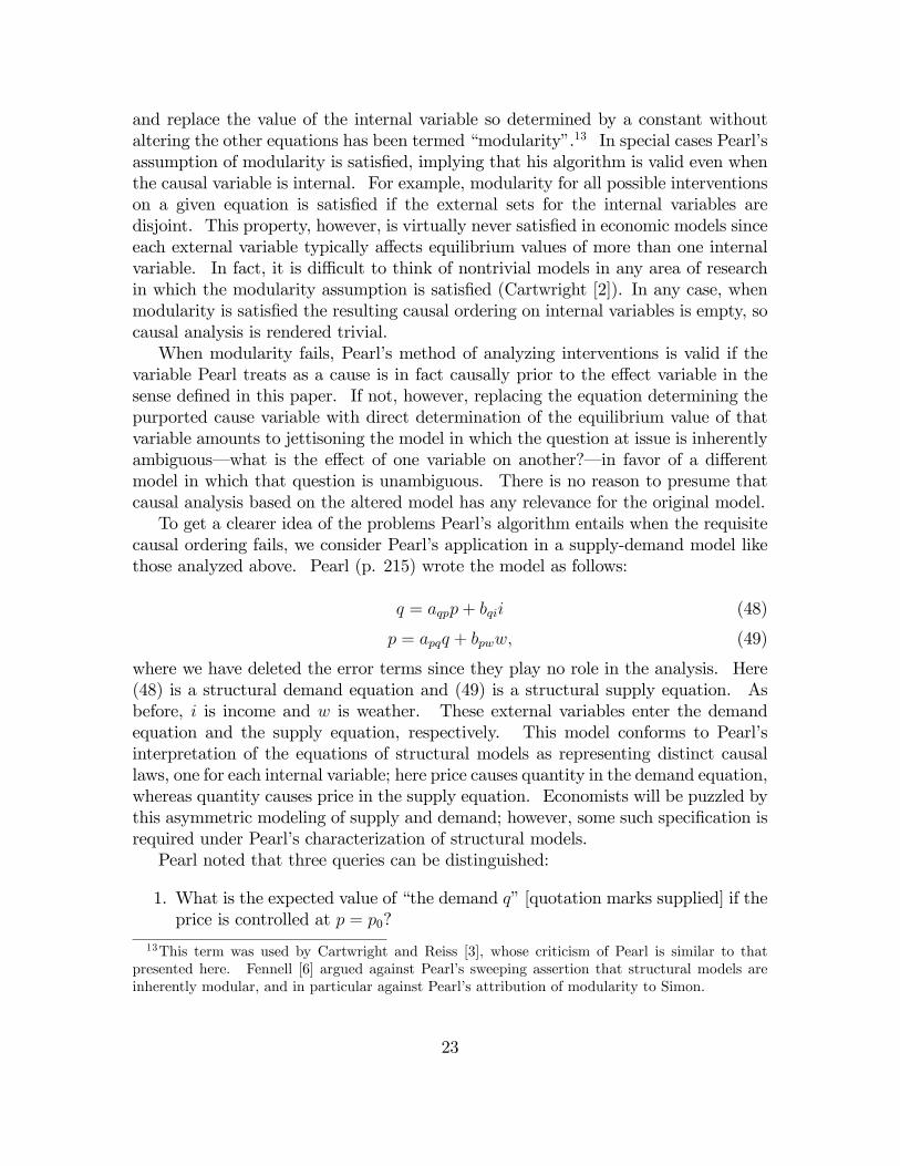
causal ordering fails, we consider Pearl�s application in a supply-demand model likethose analyzed above. Pearl (p. 215) wrote the model as follows:

q = aqpp+ bqii (48)

p = apqq + bpww; (49)

where we have deleted the error terms since they play no role in the analysis. Here(48) is a structural demand equation and (49) is a structural supply equation. Asbefore, i is income and w is weather. These external variables enter the demandequation and the supply equation, respectively. This model conforms to Pearl�sinterpretation of the equations of structural models as representing distinct causallaws, one for each internal variable; here price causes quantity in the demand equation,whereas quantity causes price in the supply equation. Economists will be puzzled bythis asymmetric modeling of supply and demand; however, some such speci�cation isrequired under Pearl�s characterization of structural models.Pearl noted that three queries can be distinguished:

1. What is the expected value of �the demand q�[quotation marks supplied] if theprice is controlled at p = p0?

13This term was used by Cartwright and Reiss [3], whose criticism of Pearl is similar to thatpresented here. Fennell [6] argued against Pearl�s sweeping assertion that structural models areinherently modular, and in particular against Pearl�s attribution of modularity to Simon.

23

2. What is the expected value of �the demand q� if the price is reported to bep = p0?

3. Given that the current price is p = p0, what would be the expected value of�the demand q�if we were to control the price at p = p1?

Observe the syntax here: despite Pearl�s terminology, the symbol q refers to (equi-librium) quantity, which equals quantity demanded and quantity supplied equiva-lently, as above. Pearl�s use of the phrase �the demand q�re�ects his speci�cationthat quantity is determined by price in the demand equation (48). In contrast, pricedetermines quantity in the supply equation (49). One wonders whether Pearl wouldaccept the question �What is the expected value of �the supply q�if the price is con-trolled at p = p0?�as being equivalent to question 1, on the grounds that quantitydemand equals quantity supplied in equilibrium, or whether instead he would regardthat question as inapplicable in the system (48)-(49), in which supply quantity is acause of price, not an e¤ect.In a footnote Pearl reported that he has presented this model and these questions

to well over one hundred econometrics students and faculty. He found that therespondents had no trouble answering 2, but only one person could solve 1, and nonecould solve 3. With the exception of the one respondent who could answer question1 to Pearl�s satisfaction, this is exactly the response pattern that one would hope forbased on the analysis of this paper: if the unsatisfactory phrase �the demand q�isreplaced by simply �q�, the correct response to questions 1 and 3 is that they areambiguous because price does not cause quantity in the system (48)-(49).Under Pearl�s algorithm, however, questions 1 and 3 are not ambiguous. They

are answered by deleting (49) and replacing it with the equation p = p0 or p = p1,respectively. Thus the relevant causal parameter is aqp; the supply elasticity apq byassumption plays no role.These di¢ culties arise because, as we have seen, Pearl�s representation of an

economic model di¤ers in key respects from the representation of a model whichmost economists would feel comfortable working with. In contrast to Pearl�s view,we have argued that de�ning �structural� models as models that directly encodecausal ideas is a dead end.

3.3 Heckman

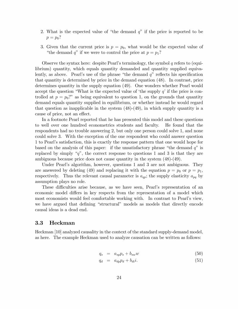
Heckman [10] analyzed causality in the context of the standard supply-demand model,as here. The example Heckman used to analyze causation can be written as follows:

qs = aspps + bsww (50)

qd = adppd + bdii: (51)

24

This structure is similar to (17)-(18) above except that the supply price ps is distin-guished from the demand price pd: Because the two equations of this model have nocommon variables, they can be analyzed separately. Heckman did so: he interpretedasp as measuring the causal e¤ect of ps on qs, just as bsw measures the causal e¤ectof w on qs: The interpretation of the demand function is similar.In characterizing equilibrium the equations for supply and demand are combined

by appending the identities ps = pd = p and qs = qd = q: Note the contrast betweenthis treatment and that proposed here. We have analyzed causation from the systemas a whole, whereas Heckman analyzed causation from each equation taken separately.Heckman was explicit about this:

If prices are �xed outside of the market, say by a government pricingprogram, we can hypothetically vary pd and ps to obtain causal e¤ects for(50) and (51) as partial derivatives or as �nite di¤erences of prices holdingother factors constant (p. 10; emphasis in original).

Under the de�nitions proposed here, the parameter asp is not associated with causa-tion because, with ps = pd = p and qs = qd = q added to the model, p does not causeq: Rather, these variables are determined simultaneously.In this example Heckman treated ps and pd as external variables for the purpose

of analyzing causation, even though p is internal when the equilibrium conditions areimposed. This treatment leads to puzzles. For example, suppose the equations arerenormalized on prices rather than quantities (as observed in note 1, it is not clearthat Heckman would accept the renormalized version of this equation as equivalentto the original version).. Then would the parameter 1=asp be interpretable as measuring the e¤ect of qs

on ps? Can asp measure the e¤ect of ps on qs at the same time as 1=asp measures thee¤ect of qs on ps, or do we have to choose? Either way, under Heckman�s treatmentthere appears to be no asymmetry involved with causation. Causal orderings areno longer orderings in the mathematical sense. In contrast, the treatment here isfully in the spirit of simultaneous-equations modeling; a supply-demand model withboth price and quantity as internal variables is a di¤erent animal from a demand (orsupply) equation with price taken as external, and one cannot substitute one for theother in analyzing causation.

4 Conclusion

In this paper we have presented a relatively detailed exposition of the received Cowlesaccount of causation in social science models, together with a rationale for the Cowlestreatment of causal orderings as stating conditions under which interventions are orare not unambiguous. Also, we have compared the Cowles analysis of causalitywith more recent discussions, concluding that the more recent discussions di¤er in

25

essential respects both from the Cowles treatment and from each other. Consideringthat it is exactly the purpose of social science models to provide a framework for thedisciplined analysis of causation, this is not a very satisfactory situation. One hopesthat analysts with an interest in philosophical inquiry will try to pull together thesevarious lines of thought in the analysis of causal structure.

References

[1] Nancy Cartwright. Probabilities and experiments. Journal of Econometrics,67:47�59, 1995.

[2] Nancy Cartwright. Measuring causes: Invariance, modularity and the causalMarkov condition. reproduced, London School of Economics, undated.

[3] Nancy Cartwright and Julian Reiss. Uncertainty in economics: Evaluating policycounterfactuals. reproduced, CPNSS, London School of Economics, 2003.

[4] Robert F. Engle, David F. Hendry, and Jean-Francois Richard. Exogeneity.Econometrica, 51:277�304, 1983.

[5] Damien J. Fennell. Comments on Stephen LeRoy�s �Causality in Economics�.reproduced, London School of Economics, 2004.

[6] Damien J. Fennell. Causality, mechanisms and modularity: Structural modelsin econometrics. reproduced, London School of Economics, 2006.

[7] Franklin M. Fisher. The Identi�cation Problem in Econometrics. Krieger, NewYork, 1976.

[8] Clive W. J. Granger. Investigating causal relations by econometric models andcross-spectral methods. Econometrica, 37:424�438, 1969.

[9] Daniel M. Hausman. Causal Asymmetries. Cambridge U. P., Cambridge, 1998.

[10] James J. Heckman. Causal parameters and policy analysis in economics: Atwentieth century retrospective. National Bureau of Economic Research, 1999.

[11] James J. Heckman. The scienti�c model of causality. Reproduced, University ofChicago, 2004.

[12] William C. Hood and Tjalling C. Koopmans, editors. Studies in EconometricMethod. John Wiley and Sons, Inc., 1953.

[13] Kevin D. Hoover. The causal direction between money and prices. Journal ofMonetary Economics, 1991.

26

[14] Kevin D. Hoover. Causality in Macroeconomics. Cambridge University Press,Cambridge, 2001.

[15] Kevin D. Hoover. The Methodology of Empirical Macroeconomics. CambridgeUniversity Press, Cambridge, 2001.

[16] Kevin D. Hoover. Nonstationary time series, cointegration, and the principle ofthe common cause. British Journal of the Philosophy of Science, 54:527�551,2003.

[17] Edward E. Leamer. Vector autoregressions for causal inference? volume 22.Carnegie-Rochester Conference Series on Public Policy, 1985.

[18] Stephen F. LeRoy. Causal orderings. In Kevin D. Hoover, editor, Macroecono-metrics: Developments, Tensions and Prospects. Kluwer Academic Publishers,1995.

[19] Stephen F. LeRoy. On policy regimes. In Kevin D. Hoover, editor, Macroecono-metrics: Developments, Tensions and Prospects. Kluwer Academic Publishers,1995.

[20] Robert E. Lucas. Econometric policy evaluation: A critique. In Karl Brunnerand Allan H. Meltzer, editors, Carnegie-Rochester Conference Series on PublicPolicy. North-Holland, 1976.

[21] JacobMarschak. Economic measurement for policy and prediction. InWilliam C.Hood and Tjalling C. Koopmans, editors, Studies in Econometric Method. JohnWiley and Sons, Inc., 1953.

[22] Judea Pearl. Causality: Models, Reasoning and Inference. Cambridge UniversityPress, Cambridge, 2000.

[23] Hans Reichenbach. The Direction of Time. University of California Press, Berke-ley, 1956.

[24] Glenn Shafer. The Art of Causal Conjecture. Cambridge University Press, Cam-bridge, 1996.

[25] Herbert A. Simon. Causal ordering and identi�ability. In William C. Hood andTjalling C. Koopmans, editors, Studies in Econometric Method. John Wiley andSons, Inc., 1953.

[26] Christopher A. Sims. Exogeneity and causal ordering in macroeconomic mod-els. In Christopher A. Sims, editor, New Methods of Business Cycle Research:Proceedings from a Conference. Federal Reserve Bank of Minneapolis, 1977.

27