causal effects of maternal time-investment on children’s
TRANSCRIPT
Causal Effects of Maternal Time-Investment on
Children’s Cognitive Outcomes∗
Benjamín Villena-Roldán
University of Chile†
Cecilia Ríos-Aguilar
Claremont Graduate University‡
December 18, 2011
∗We thank Amy Hsin, Sandra Hofferth, Frank Stafford, Almudena Sevilla, Giacomo de Giorgi, Alejandra Mizala,Eugenio Giolito, Dante Contreras, Jeanne Lafortune, as well as participants of conferences at University of Maryland,University of Michigan, 2011 LAMES-LACEA, University of Chile, and ILADES-Georgetown. We thank AndreaTartakowsky for her research assistance.
†Center for Applied Economics. Corresponding author email:[email protected] . This research has receivedfinancial support fromCentro de Investigación Avanzada en EducaciónBicentenario Project CIE-05 grant.
‡School of Educational Studies. email: [email protected]
1

Abstract
Many social scientists hypothesize that the time mothers spend with their children is crucial
for children’s cognitive development. Unlike most studiesthat investigate maternal employ-
ment effects on children, we estimate direct causal effectsof time-diary measured maternal
time using the CDS - PSID dataset. Considering maternal timeallocation endogenous, the
effect of an increase of maternal time associated with a risein childcare price (IV estimate) is
an order of magnitude larger than OLS estimates for Applied Problems and Word-Letter Iden-
tification tests. Evidence also shows that the effect is larger for children living with college-
educated mothers and in two-parent households.
Keywords: Children outcomes, maternal time-investment, causal effect, Instrumental Vari-
ables.
JEL codes: D1,J13,C36.
1 Introduction
What is the best way parents can use their time with their children? A longstanding and reasonable
hypothesis in social sciences is that parents have, potentially, a large influence over the outcomes of
their offspring. In addition to the well-deserved practical and scientific interest on this topic, there
is also a recent literature showing that children’s outcomes are, in turn, key determinants of future
adulthood outcomes, including earnings (Danziger and Waldfogel 2000; Heckman et al. 2006) and
health (Currie et al. 2008). Despite the importance of the time parents and children spend together,
available empirical evidence about itscausaleffects on children is surprisingly scarce. The main
contribution of our paper, then, is to estimate the causal effects of time-diary measured maternal
time-investment on several cognitive outcomes using a simple empirical model of human capital
accumulation.
Some of the existing scholarship1 that examines the impact of maternal labor force participation
1See the literature review section for a thorough discussionon this topic
2
or hours worked on children’s outcomes interprets maternalemployment as an indirect measure
of maternal time-investment on children. Our approach differs in three specific ways from this
vast literature. First, since the relationship between thenumber of hours worked and time mothers
devote to their children is weak at best, we use time-diary data to obtain direct estimates of the time
mothers and children spend together. Even though time-diary data shows that working mothers
devote slightly less total time to children, most of the maternal time used at work is offset by
housework and leisure (Hill and Stafford 1985; Datcher-Loury 1988; Sandberg and Hofferth 2001).
Second, as described in Section 3, we find evidence that thereis a great deal of heterogeneity in
maternal childcare time allocations across different demographic groups of mothers. Hence, there
is an important identification issue of the maternal work “treatment” since its impact could be either
generated by changes of quantity or composition of maternaltime, or by heterogeneous responses
of children to a change in maternal time-investments. Third, we estimate a simple theoretical
model of human capital to surmount these issues. Our framework considers that maternal time-
investment is endogenously determined, has a cumulative impact on children outcomes, and affects
children in heterogeneous ways.
Several data requirements need to be met to properly estimate the causal effects of interest in
this paper: (1) a longitudinal database with information onchildren’s outcomes, (2) reliable records
of mother-child shared time, and (3) measures of family background for a group of individuals
over time. The Child Development Supplement (CDS) (waves I,II and III) merged with the Panel
Study of Income Dynamics (PSID) provides us with such a special data combination. Using the
CDS-PSID data has many advantages. First, instead of using potentially biased self-reported and
inaccurate maternal time use, we employ the Time Diaries (TD) data to directly measure maternal
time investments. More specifically, the TD data include thetype and duration of various kinds of
activities in which mothers and children engage together. Second, we can also examine the causal
effects of different activity categories (e.g., total and educational) and of distinct levels of maternal
involvement (i.e., “active” or directly participating in the activity versus “passive” or being around
during child’s activity). Finally, the PSID contains valuable historical and demographic data on
3

mothers (and households) that may also exert an influence on children’s outcomes, and therefore
can be used as statistical controls.
We propose a simple framework of human capital accumulationbuilt by maternal time-investment,
which implies a theoretical relationship betweenchangesin outcomes and maternal time-investments
levels. However, although maternal time allocation affects children’s outcomes, the causality may
also run in the opposite direction. That is, mothers usuallydevote more time to children whose
academic achievement is low. Hence, inputs are essentiallyendogenous (Todd and Wolpin 2003;
Cunha and Heckman 2008). Given the existing endogeneity, the causal effects are difficult to es-
timate. Out of several possible exogenous sources of maternal time variation, in this paper, we
focus on predicted childcare prices. To obtain them, we estimate an equation of the childcare
price2 using the panel sample-selection model of Wooldridge (1995). Next, we estimate the ef-
fect of maternal investment on children’s outcomes using a Fixed-Effects Instrumental Variables
estimation technique. This identification strategy is valid if the variation in childcare prices solely
affects children through the substitution of day care time for maternal time, holding constant family
background characteristics. We find this to be a very plausible claim. Moreover, Kimmel and Con-
nelly (2007) document that mother-child shared time increases when the predicted childcare price
raises. Our first-step estimates are consistent with their results, and also show that the maternal
response to childcare prices declines with child age. Furthermore, we also take care of the possible
weakness of the instruments used by (1) estimating the modelutilizing the Limited Information
Maximum Likelihood (LIML) estimator, substantially less biased than the traditional Two-Stage
Least Squares (Stock et al. 2002), and by (2) reporting the Cragg and Donald (1993) test for weak
instruments as suggested by Stock and Yogo (2005). We interpret our estimates as a Local Average
(marginal) Treatment Effect, that is, the marginal averageimpact of a rising maternal-investment
in response to a childcare price increase in a particular sub-population of children (Imbens and
Angrist 1994).
Our findings largely support the hypothesis of endogenous maternal time-investment alloca-
2For details, please see Appendix 2
4

tion because LIML estimates are an order of magnitude largerthan OLS for Applied Problems and
Word-Letter Identification cognitive tests. Moreover, since IV estimates are biased towards OLS,
the level of bias (10-20%) consistent with Stock and Yogo (2005) critical values of the Cragg-
Donald statistic becomes secondary because LIML estimatesare roughly 10 to 20 times larger
than OLS. By estimating the results for different sub-populations3, we find that children living
with college-educated mothers and in two-parent homes benefit the most from the exogenous vari-
ation in maternal time-investment. This suggests that marginal substitution of maternal time by
formal child care should be beneficial in terms of those outcomes, which is consistent with previ-
ous evidence (Brooks-Gunn, Han, and Waldfogel 2002; Ruhm 2004). The magnitude of the effect
of increasing total average maternal time by 1% per year is similar to the impact of joint maternal
employment and day care placement estimated by Bernal and Keane (2008, 2010). While the ef-
fects of total active maternal time and of educational time are also significant and much higher than
OLS for Applied Problems and Word-Letter Identification , their magnitude is lower than the one
estimated for total maternal time-investment. In addition, our results show a less clear impact of
an increase in maternal time-investment on Passage Comprehension and Digit Span tests. Finally,
the results related to certain sub-populations are less reliable because our instruments are not so
strong in some cases.
Findings from this study have policy implications. First, childcare subsidies and regulations
should take into account the cost involved in maternal time allocation decisions on the child’s cog-
nitive abilities. Second, schools need to consider the compensatory and complimentary efforts of
families in producing higher cognitive achievement. Educational policies should explicitly con-
sider the role of mothers and household socioeconomic conditions in children’s skill formation
process.
The rest of the paper is organized as usual. Section 2 discusses the related literature. We
describe the databases and present some descriptive statistics, emphasizing the weak connection
between maternal employment and maternal time-investmentin the data in Section 3. We present
3based on child’s gender, child’s race, mother’s educational background, and child’s living arrangement
5

the model, and discuss estimation and identification in Section 4. The results and the related
discussion are in Section 5. We conclude in Section 6.
2 Literature Review
Our paper is primarily related to the vast literature in sociology, psychology, economics, and edu-
cation that studies the effects of maternal time-inputs on children’s cognitive outcomes. As men-
tioned before, since effective mother-child shared time ishard to observe, in practice most of the
studies have focused on the effect of maternal employment. Bernal and Keane (2008, 2010) pro-
vide a good summary of the literature in this area. Accordingto them, there is no consensus on the
effect of maternal employment on children’s cognitive outcomes. Previous research has failed to
acknowledge the impact of earlier time-investments on children’s cognitive development, as well
as the inevitable sample selection of mothers into employment. Very few scholars have recognized
the inherent reverse causal relation between children’s outcomes and maternal time and good in-
puts. Using IV and OLS techniques, Blau and Grossberg (1992)find a negative impact of early
maternal employment, but a potential offsetting effect later in life. James-Burdumy (2005) find
little evidence of negative effects on children’s cognitive development using IV and fixed-effects
procedures. Bernal and Keane (2008) use different IV techniques, and Bernal (2008) and Bernal
and Keane (2010) estimate a micro-founded structural modelto find a significant effect of negative
impact of maternal employment associated to day care placement. Hill and O’Neill (1994) find
that an increase of hours worked has a negative effect on children’s outcomes, but this effect is
partially offset by higher income. Neidell (2000) find that maternal work has a detrimental effect
on cognitive and non-cognitive outcomes, even though the effect is greater for working mothers.
Waldfogel et al. (2002) find a negative impact of very early maternal employment. Brooks-Gunn
et al. (2002) and Ruhm (2004) find that maternal employment isharmful to children’s cognitive
outcomes, especially for children of highly educated mothers.
An evident difficulty of the latter literature is the fact that the link between maternal employ-
6

ment and maternal time devoted to children is quite weak, as ashown in empirical studies on ma-
ternal time allocation. A robust finding is that maternal time devoted to children has not changed
that much in the last decades despite the rise in maternal labor force participation (Bianchi 2000).
Gauthier, Smeeding, and Furstenberg (2004) look at data from several countries and find that paid
work seems not to crowd-out child-parent shared time. Moreover, mothers and fathers are increas-
ing childcare time in absolute terms. Monna and Gauthier (2008) review evidence showing that
most of mother’s hours worked displaces housework and leisure, with a slight effect on childcare.
Moreover, Bryant and Zick (1996) report that employed mothers devote more time to children in
shared housework and leisure activities. Zick, Bryant, andÖsterbacka (2001) find that employed
mothers engage in reading/homework activities more frequently than nonemployed ones, although
Cawley and Liu (2007) find a lower chance of being involved in educational activities with children
of working mothers in the ATUS data.
On the other hand, there is strong evidence showing that moreeducated parents devote more
total time to their offspring (Datcher-Loury 1988; Bryant and Zick 1996; Kimmel and Connelly
2007) as well as more time in developmental activities despite maternal employment (Sandberg
and Hofferth 2001; Craig 2006). Guryan, Hurst, and Kearney (2008) examine international data
to conclude that families with high levels of income and education devote substantially more time
to childcare in all the countries studied and within countries. In contrast, other time uses such
as leisure and housework decrease with income and education. This suggests that the correlation
between employment status and childcare depends on observable characteristics of the household.
We present some evidence of this below.
There are few studies that use direct measures of maternal-child shared time as a determinant
of children’s outcomes. Hsin (2009) summarizes this scant empirical literature that roughly finds
no significant correlation between children’s outcomes andthe time mothers devote to them. These
results are misleading because those papers do not properlyaccount for heterogenous backgrounds
or address endogenous inputs. Hsin (2008) finds that maternal time-investment has a positive
impact on children’s outcomes, but only among mothers with high literacy levels. Carneiro and
7

Rodrigues (2009) use generalized propensity score matching to estimate the “dosage” effect of
maternal time, but neglect the effects of cumulative inputson a child’s cognitive achievement.
Del Boca, Flinn, and Wiswall (2010) develop and estimate a structural microeconomic model with
specific functional forms for preferences, child outcome production technology, and time and bud-
get constraints using data from the CDS. Their model and policy experiments focus primarily on
the trade-off between hours worked and household income. Nevertheless, they neglect empirically
important time-use buffer activities such as leisure and housework.
We explicitly address the importance of cumulative time andgoods inputs, unobserved time-
invariant heterogeneity, and contemporaneous input endogeneity by using a simple human capital
model. Our approach is related to the existing literature onchild skill formation, also known as
outcome production function. Under this perspective, the time parents spend with children is an
investment that directly stimulates cognitive development and provides an emotionally-, ethically-,
and intellectually-rich environment for their children that promotes learning and positive behaviors.
Todd and Wolpin (2003) and Cunha and Heckman (2007, 2008) (and subsequent papers) propose
a theoretical and empirical framework for children skill formation based on dynamic unobserved
skills or factors. Almond and Currie (2010) use a similar framework to organize empirical findings
of children’s academic achievement before age five. Cunha and Heckman’s approach suggests
that unobserved factors interact, simultaneously, with parental time-investments and with family
background to determine children’s outcomes. In contrast,our approach is more direct, since our
ultimate goal is to estimate the causal effect of maternal time-investment on children’s cognitive
outcomes, without a very specific stance on the presumed underlying technology. Given our goal,
the approach we take is closely in line with the work by Bernaland Keane (2008), which relies on
a more direct and theoretically sound empirical specification.
3 Data
In this section, we describe the databases we use in our investigation.
8

Child Development Supplement (CDS) The CDS is a supplementary survey of the Panel
Study of Income Dynamics . In 1997, the PSID supplemented itsdata with additional informa-
tion on the sample of PSID parents and their 0-12 year-old children to generate a longitudinal
data base of children and their families. Out of the 2,705 families selected for the CDS-I, 2,394
families (88%) participated, providing information on 3,563 children. In 2002-2003, CDS re-
contacted families in CDS-I who remained active in the PSID panel as of 2001. CDS-II success-
fully re-interviewed 2,017 families (91%) who provided data on 2,908 children/adolescents aged
5-18 years. CDS-III data was collected in 2007. A great deal of the original sample in 2007 was
ineligible due to being 18 or older.
From the CDS longitudinal data, we use the following information: (1) age-graded assessments
of the cognitive and behavioral outcomes of each child such as Woodcock-Johnson Applied Prob-
lems (math), Passage Comprehension , and Word-Letter Identification tests (Woodcock, Johnson,
and Mather 1989). In this paper we also study the impact of maternal time on the WISC Digit Span
test (short-term memory) (Wechsler 1974). We extract demographic characteristics of the children
which are supplemented with their PSID Individual records.Finally, we obtain measures of Home
Quality Index , which is constructed from an observational assessment of the CDS interviewer.
The details are explained in Appendix 3.
Time Diaries (TD) Researchers are often interested in measuring time devotedto certain
activities over a period of time, such as the amount of hours per day that parents spent on a variety
of activities with their children. Time diary collection isthe preferred way to measure actual time
use of individuals (Juster and Stafford 1991). The observation methods are very costly, intrusive,
and limited in the amount of a day that can be covered (Juster 1985). Retrospective recall surveys
that consist of the type and frequency of activities tend to provide inaccurate measurement of actual
time uses (Robinson 1985). Hofferth (1999) shows that parents, especially the highly educated,
tend to overstate the time they spent on “socially desirable” activities, such as helping their child
with his/her homework.
In contrast to recall surveys, considerable methodological work has established the validity
9

and reliability of data collected in time-diary form. Time diaries are a chronological report by the
child’s primary caretaker, and if sufficiently old, by the child him or herself about the child’s activi-
ties over a specified 24-hour period. In the TD data, respondents were asked to provide the detailed
time and nature of the activity in which children participated. For each activity, respondents report
(1) time the activity began and ended, (2) whether the child was watching TV or a video, (3) where
the child was doing the activity, (4) who was participating in the activity with the child, (5) who
else was with the child, but was not directly involved in the activity, and (6) what else the child was
doing during the primary activity. One of the most importantadvantages of the TD data a is that
total time in one day has to add to 24 hours. Consequently, while individual times may be slightly
inaccurate, the times are consistent with one another. The disadvantage of the TD data is that it
represents only a sample of children’s days. As such, it has limited reliability. To ameliorate this
problem, the CDS-TD collects time diaries of one weekday andone weekend day. We construct
the total time a mother devotes to her child by weighting weekdays by five and weekend days by
two.
The TD data contained in the CDS is very extensive. There are approximately 600 primary
activities that were aggregated into 11 major categories. In this paper, we focus on the education-
oriented activities, which include only those labeled as educational and professional training (e.g.,
doing homework, taking classes, courses or lectures outside of school, etc.). Thus, we use two
broad time categories: (1) total time spent on all activities, and (2) total time spent on educationally-
oriented activities4 (Yeung et al. 2001).
We are also interested in examining potential differences that may arise when parents are ac-
tively involved in the activities versus when they are not. Consistent with our interest, Folbre
et al. (2005) argue that it is important to make the distinction between “active” and “passive”
time-investments because they may influence children’s outcomes in different ways. The Time
Diaries allows us to distinguish between these distinct levels of involvement. More specifically,
we define active time as the time the mother spends directly involved in an activity, and passive
4We thank Sandra Hofferth for sharing these data with us.
10

as the time she spends with her child being just “around” the activity. To aid in the interpretation
of our analysis, we use the last two criteria to construct four variables reflecting maternal time
investment: (1) Total maternal time, (2) total maternal time active, (3) educational maternal time,
and (4) educational maternal time active.
Panel Study of Income Dynamics (PSID) The PSID is a longitudinal study of a represen-
tative sample of U.S. individuals and their families. Since1968, the PSID has collected data on
family composition changes, marriage and fertility histories, employment, income, time spent on
housework, health, and many others. The sample size has grown from 4,800 families in 1968 to
more than 7,000 families in 2001. For this particular paper,the PSID data was used in two spe-
cific ways. First, we use the PSID Family records for maternaleducation, maternal age5, family
income, childcare expenditure, family structure, reported hours worked and housework hours.
Current Population Survey (CPS) The Current Population Survey March data was used to
construct labor market and welfare variables that may generate an exogenous source of variation in
maternal time use allocations. We consider several local labor markets variables that may influence
maternal time-allocation decisions. We collected data on average child benefits by year and state,
and wages of childcare occupation workers by year and state for the period 1990-2007.
3.1 Descriptive statistics
Children outcomes and family background Standardized cognitive outcomes scores vary
a great deal according to child gender and maternal education. These differences are meaning-
ful since all measures of children’s cognitive outcomes areordinal scales that allow comparisons
within the same test (but not between them). Panel A of Table 1show that the children in the
sample exhibit a slight decreasing pattern for the Applied Problems , Passage Comprehension and
Word-Letter Identification tests. We do not have an explanation for these patterns. We notice that
female children perform better than males in all four tests,for ages 5 to 11. For children older than
5We checked the consistency of maternal educational attainment and maternal age for several years. We alsosupplement these family variables with PSID Individual files in order to minimize the missing observations. Thedetails of the procedures applied are available upon request.
11
11, females still outperform males except on the Applied Problems test. Looking at Panel B, it is
apparent that children of highly educated mothers perform substantially better than children of low
educated mothers in all tests. Panel C shows that children from part-time workers have higher test
scores than either full-time employed and non-employed mothers. In turn, the children of these
last two groups of mothers have similar scores.
The Table 2 shows little systematic differences between thehouseholds of boys and girls in the
sample, except for the fact that actual expenditure in childcare for young girls is considerably larger
than the amount spent on boys of the same age. The sample also shows that the group of older
children has a larger share of Black children and a lower share of White children in comparison to
the youngest group. The share of households with female heads is notably larger for children older
than 11, probably because of the higher frequency of divorceonce children get older. The number
of other adults at home also increases with a child’s age, as well as the value of the house in which
they live.
Table 2 also shows that highly educated mothers are roughly 3.5 years older on average. House-
holds with a highly educated mother have a larger proportionof White children and male heads.6
Home quality,per capitafamily income, and books per child are higher for more educated moth-
ers. The predicted childcare cost is higher for more educated mothers on average, and so it is the
actual childcare expenditure. There is also a striking difference between highly and low educated
mothers in regards to the value of the house. Indeed, a great deal of the difference is driven by the
fact that these statistics are computed using a house price of one cent if the family does not own a
house.7
Mothers greatly differ according to their working status. We observe that full-time working
mothers are more educated, on average, than mothers who workpart-time. Mothers who work part-
time are also more educated than non-working mothers. Part-time working mothers tend to have
more White children and to live with a male partner more frequently in the sample. Interestingly,
6This claim uses the standard PSID convention that defines a household head to be any male older than 18 yearsold at home.
7We report log(value house +0.01)
12

a larger share of mothers working full-time are household heads. Full-time working mothers tend
to live in households with a relatively higher Home Quality Index andper capitafamily income.
Regarding childcare costs, our estimates show that it is 0.2log points larger for working mothers
with respect to the non-working ones. Nevertheless, the actual childcare expenditure of full-time
working mothers almost doubles the amount spent by mothers working part-time. Finally, part-
time working mothers live in households that are 0.17 log points more valuable than full-time
working mothers (these numbers include the zeroes of “no-owner” status.
Maternal employment vs maternal time-investment While many studies have found that
employed mothers devote less time to their children than their non-working counterparts, it is
clear that other activities such as housework and leisure, are the ones that are drastically reduced
to accommodate the number of hours worked (Guryan, Hurst, and Kearney 2008). Aguiar and
Hurst (2007) documented that over the last decades several categories of total maternal childcare
time have increased as well as total hours worked. These timeuses have increased as a result of
declining housework hours.
A set of scatter plots in Figure 2 reveal that maternal hours worked are weakly and negatively
correlated with each one of the time use categories we analyze here (total maternal time, total
maternal time active, total educational time, and total educational time active). However, the dis-
persion around the local polynomial regression lines is substantial.8 This evidence suggests that
maternal hours worked is, at best, a very noisy proxy of maternal time-investment. We also find a
positive association between housework time and maternal time-investment categories, but again,
the conclusion is that the latter time use category is a very noisy measure of the time mother and
child engage in together.
Nevertheless, our skepticism on using maternal employmentas a measure for maternal time in-
put goes beyond this issue. There is substantial evidence showing that the time allocation of work-
ing mothers varies by educational patterns, child age, and gender (Datcher-Loury 1988; Bryant
and Zick 1996; Yeung et al. 2001 among many others). The economic literature9 has considered
8For details, see on the footnotes of Figure 29Aguiar and Hurst (2007) provides a more complete discussionon the conceptual distinction between childcare
13

childcare as a separate time category which is distinct fromleisure and housework not only on the-
oretical grounds, but also because it behaves differently in response to exogenous shocks such as
changes in childcare price and wages. For instance Kimmel and Connelly (2007) show that while
leisure and housework decrease in predicted wages, maternal childcare time increases. Ignoring
these issues would lead to misleading conclusions.
Maternal time allocation substantially varies across groups defined by child age, gender, and
maternal education. In Table 1 we observe average total maternal time is higher for male children
when their age ranges 5-11, but the pattern reverses for female children older than 11. The time
allocation for narrowly defined activities such as educational active is not gender-biased. When
we look at the maternal education gradient, we do observe that highly educated mothers devote
more time to children but these differences seem less important for more specific time categories.
Finally, Panel C of Table 3 shows us that maternal employmentreveals little about time allocation.
While non-employed mothers provide more total hours to children, the differences across groups
suggests that most of the hours worked have displaced other time categories such as leisure and
housework. A remarkable finding is that mothers working part-time actually provide more hours
to total active childcare and to educational activities.
Table 3 shows pairwise correlations between maternal hoursworked and mother-child shared
time for different subsamples. We observe that the negativecorrelation between hours worked
and maternal time-investment decreases as we consider morespecific time uses. Moreover, the
negative correlation seems larger (in absolute terms) for younger, male children with low educated
mothers.
This evidence reassures our skepticism on evidence regarding maternal employment “treat-
ment” effects. Our concern is not only that hours worked or employment status is a very noisy
proxy for maternal time devoted to children, but that the evidence also indicates that the link be-
tween the two variables weakens as we focus on more active types of maternal time-investment.
The fact that the correlation consistently varies according to child gender, child age, and maternal
time and housework
14

education suggests that the maternal employment is a very different treatment across groups. This
also implies that the noisiness of maternal time cannot be treated as a textbook measurement error
problem. Since classic measurement error biases estimatestowards zero, each subsample provides
estimates with a varying level of bias. To summarize, we see asevere identification problem: ma-
ternal employment heterogeneity effect. This effect may bedue to: (i) working mothers actually
provide a different level or composition of time-investment, or (ii) certain groups of children may,
intrinsically, be more sensitive to maternal time-investment. Metaphorically, maternal employment
is a cocktail of a varying number of pills of several possiblekinds that is administered to heteroge-
neous patients. In addition, the drugs are administered using a varying degree of uncertainty that
depends on the patient’s condition. Clearly, little could be learned from this poor experimental
design.
4 Model
There are several approaches in the literature to model children’s outcomes development. Cunha
and Heckman (2007, 2008 and subsequent papers) focus on the dynamic evolution of unobserved
skills that are identified as dynamic factors. Our approach here is closer to Bernal and Keane (2008)
since it establishes a more straightforward relation between observable inputs and outcomes, with-
out a mediating role of unobserved factors.
Despite the fact that the model we propose is non-linear in deep parameters (because of the
unobservable maternal time-investment), we can recover the parameters of interest by estimating
a linear model. After presenting the model and recognizing the potential endogeneity problem,
we examine the potential sources of exogenous variation –notably, childcare price variation– that
can provide a reasonable identification strategy. Then, we utilize strategies in the econometric
literature to handle potential Weak Instruments problems in Instrumental Variables methods. We
implement the Limited Information Maximum Likelihood (LIML) estimator, which is less prone
to these problems (Stock, Wright, and Yogo (2002) for a survey). We also report tests for weak
15

instruments (Cragg and Donald 1993) with tabulated values from Stock and Yogo (2005).
Theoretical setup Most of the literature suggests models in which maternal time and goods
enter as an input into the production function as well as usually unobserved genetic conditions. As
noticed by Bernal and Keane (2008, 2010), only few papers recognize the importance of previous
inputs in generating current outcomes. We explicitly consider this issue in our model specification.
We postulate that there is a natural, possibly nonlinear, trend for cognitive development as
the child grows older. Nevertheless, we consider heterogeneous cognitive development profiles
that vary according to child gender, and a proxy for maternalability (as measured traditionally by
schooling). Deviations from this standard trend may be caused by higher human capital level,X,
built via maternal time-investment or by higher physical capital, K, accumulated through goods
investments.
Both capital stocks,X andK , can be written as a cumulative weighted sum of investmentsx and
k. We recognize that the marginal contribution of investments is essentially heterogenous across
children and it may be determined by factors such as maternaleducation, child gender, age, race,
and family environment variables. Notably, previous research in child development psychology
and several studies in skill-formation technology have suggested that early investments have a
stronger impact in a child’s early ages (Cunha and Heckman 2008; Almond and Currie 2010). It
is also reasonable to think that the marginal impact of maternal time-investment varies according
to her education or skills. Indeed, Hsin (2008) found that the time-investment of mothers with
high literacy skills has a positive impact on children’s outcomes, other maternal time-investments
were unproductive. Evidence of higher detrimental effectsof the employment of highly educated
mothers can be rationalized in the same way (Ruhm 2004).
We propose a reduced form linear specification for child outcomes that is expressed in the
following equation
yhn,t = αh
n +an,t
∑i=0
β hn,i +
an,t
∑i=0
γhn,ixn,i +
an,t
∑i=0
δ hn,ikn,i +uh
n,t (1)
wheret represents time and then subindex represents children in the CDS sample.
The outcomeh of child n at time t is represented byyhn,t . The termαh
n stands for an unob-
16

served environmental/genetic component of the childn that specifically affects theh-th outcome
at all ages. The coefficientsβ hn,i represent the outcome specific age-trend determining the average
development of then-th child.
The cumulative weighted sum ofxn,i is the human capital accumulated up to timet by the
child n due to maternal time-investment for outcomesh = 1,2, ...,H. Likewise, the cumulative
weighted sum ofkn,i represents the physical capital accumulated by the household n up to timet.
The coefficientsγhn,i andδ h
n represent the outcome-specific marginal effects of investmentsx and
k for the n-th child at agei. This formulation allows for marginal effects varying on the child’s
current agean,t .
Our method estimates first-differences of equation (1) to get rid of unobserved child-home het-
erogeneity. This approach is also convenient to maximize the sample size since there is substantial
non-response in the first and third waves of the CDS. Some children were too young in 1997 or too
old in 2007 to take the cognitive tests. Since the CDS reportstime use every 5 years, the 5-year
variation can be written as
∆5yhn,t =
an,t
∑i=an,t−5
β hn +
an,t
∑i=an,t−5
γhnxn,t +
an,t
∑i=an,t−5
δ hn,ikn,t +∆5uh
n,t (2)
The logical implication of this setup is that accumulated maternal time-investment between the
two dates is the key determinant of changes in children’s outcomes. One important limitation is
that we do not observe these investments in every moment of time in the CDS data. We need to
make additional assumptions on the way mothers behave in order to identify the impact of maternal
time-investment on the outcomeh. We assume that both investment data we observex∗n,t andx∗n,t−5
are related to the unobserved time-investments in the following way
xn,t = ξn+ρxn,t−1+en,t (3)
This equation shows that the maternal time allocation at time t depends on child and family un-
observed factorsξn, the choice of maternal investment in the previous period and a random shock
17

en,t . We can get rid of the unobserved family effect by taking first-differences in the equation (3)
∆xn,t = ρ∆xn,t−1+∆en,t
xn,t −µxn,t−1+(1−µ)xn,t−2 = ∆en,t with µ ≡ 1+ρ
Using equations fort, t − 1, t − 2 andt − 3 we formulate a 4× 4 linear system whose detailed
solution is shown in . Once solved, every period time-investment can be written as
xn,i = λix∗n,t +(1−λi)ix
∗n,t−5+
t
∑j=t−3
τ j ,ien,t− j ∀i = t −4, ..., t−1
We assume the effect of maternal time-investment can be decomposed asγn,i = φnφi whereφn
is a child-household specific component andφi is a child-age specific component. The expected
change in human capital stock can be expressed as
∆5Xhn,t =
t
∑i=t−4
γhn,ixn,i =
t
∑i=t−4
γhn,i
(
λix∗n,t +(1−λi)x
∗n,t−5
)
+ τe
= γhnΛx∗n,t + γh
n (5−Λ)x∗n,t−5+ τe
with Λ =5∑t
i=t−4 λiγn,i
∑ti=t−4γn,i
=5∑t
i=t−4λiφi
∑ti=t−4φi
andγn =15
t
∑i=t−4
γn,i
The termτe is the dot product of the vector maternal time allocation shockse and its associated
coefficient. Finally, we can see that the marginal effect of the conditional expectation acrossN
children is
E
[
∂E[∆5Xhn,t
∣
∣e]
∂x∗n,t
]
= ΛE[γn] = Λγh
The conditional expected variation of maternal-time accumulated human capitalX can be ex-
pressed as the average marginal effect of maternal time-investmentx∗n,t amplified by a factorΛ,
the 5-year temporal impact of the investment.
Since goods helping child development are likely to be financed with labor income, and mater-
nal labor supplies are correlated with maternal time-investment on the child, we consider a proxy
18

for child goods in periodt −5 instead of its contemporaneous measure. By doing so, we avoid a
new source of simultaneity into the estimation. As a measureof material well-being we primarily
use the Home Quality Index . A careful description of this index is in Appendix 3. We also ex-
plore other measures of material well-being including logper capitareal household income and
the number of books of the child, although we do not notice important differences using the latter
variables. Therefore, we estimate the following generic equation
∆5yhn,t = πh
0x∗n,t +πh1x∗n,t−5+πh
2kn,t−5+πh3an,tkn,t−5+πh
4en+vhn,t (4)
We can easily recover the value ofγh by computingπh
0+πh1
5 becauseπ0 = γhΛ andπ1 = γh(5−Λ).
Identification Strategy Identification problems arise due to the potential endogeneity of
contemporaneous maternal time-investment. In our framework, this problem is equivalent to an
omitted variable bias of the time shockse. Therefore, the error of equation (4) is likely to be
correlated with the contemporaneous maternal time investmentx∗n,t . In contrast to our approach, the
literature has mostly highlighted the fact that maternal time allocation may depend on unobserved
time-invariant child characteristics. Although such an assumption may be reasonable, it is more
general to assume that maternal time allocation may depend on time-varying conditions such as
children’s outcomes (Todd and Wolpin 2003). For instance, mothers may devote more time to their
children if, for instance, they perform poorly at school, regardless of whether the low academic
achievement is caused by early disadvantage or by a negativeshock later in life.
A natural approach to solve these difficulties is Instrumental Variables estimation. As discussed
in the literature (Wooldridge 2002; Murray 2006; Angrist and Pischke 2009), we need a significant
exogenous source of variation of the maternal time allocation (i.e., instruments are not weak)
that does not directly affect children’s outcomes conditioning on other covariates (i.e., exclusion
restriction). Formally,
1. Exclusion restriction ofz: ∆yhn,t | covariates⊥ z
2. No weak instrumentsz: E [ze| covariates] 6= 0
19

We recognize that there may be plenty of heterogeneous responses of children’s outcomes to ex-
ogenous variation of maternal time induced, in turn, by a change inz. Hence, we interpret our
results as a Local Average Treatment Effect (LATE) that may depend on the particular instrument
used. As shown in this literature (Imbens and Angrist 1994; Angrist and Pischke 2009), the es-
timated effect is driven by a group of mothers who only changed the time they spend with their
children in response to a variation ofz.
We rely on a standard theory of household time allocation to find appropriate instruments. In
line with Gronau (1977), mothers decide how to split their limited time into four possible uses:
work, housework, childcare, and leisure. Our instrumentalvariables capture exogenous shocks
to the benefits and costs associated with these time use categories. Hence natural candidates for
being instruments are variables associated to (i) the cost of childcare service, (ii) the benefits and
costs of hours worked in the market, (iii) the cost of external housework provision, and (iv) the
government resources for welfare benefits, related regulations and eligibility rules. Each one of
these instruments represents exogenous variations that are essentially distinct. We prefer to use the
least number of instruments per estimation in order to interpret each result as a response induced
by distinct quasi-natural experiments. This approach is also consistent the literature of Weak In-
struments that warns of the danger of using too many instruments (Bound et al. 1995; Stock et al.
2002).
In addition of the two standard identification conditions for IV estimation, under heterogeneous
effects, we will also need to satisfymonotonicityof maternal time response toz. That is, if z
changes, then all individuals in the population of interestmust show either a weak increase or
weak decrease in the time spent with children in response to such a change. In principle, since the
household owns a time endowment, there are substitution andincome effects that work in opposite
directions. Thus, families differing in observable characteristics (wealth, age, etc) may respond to
a price change in different ways. Since the IV estimation implicitly averages the responses across
the population, then, it is possible that we could obtain a negligible effect in practice. Even though
monotonicity may not hold in practice, it is important to state that this drawback worksagainst
20

obtaining significant results.
Out of many possible instruments, we focus in this paper on the effects of childcare price
variation. While this choice is somewhat based on space considerations10, we believe that childcare
services is a direct substitute for mother-child shared time. As such, this price greatly affects the
time-use allocation considering that the total cost can be close to 1/4 of the earnings of a full-
time minimum-wage worker (Connelly and Kimmel 2003). This price consideration is likely to be
relevant for most families with children since they, unquestionably, need some minimum amount
of time-investment. Consistently with theory, Kimmel and Connelly (2007) estimated a significant
positive response of actual mother-child shared time to an increase in childcare prices. For other
time uses, we argue, it is not clear how maternal time-investment changes when other mentioned
costs and benefits adjust.
We obtain estimative child care costs using PSID historicalrecords on childcare household
expenses divided by the number of children under the age of six. Since some families do not
spend money on childcare, we need to generate a counterfactual unobserved price along the lines
of Kimmel and Connelly (2007). To do this, we use the basic insight of non-random sample
selection (Heckman 1976): old children or adult relatives at home are likely to affect the decision
of hiring external childcare services, but they do not affect the price paid once the parents send the
child to daycare. We exploit the panel dimension of the data to control for family time-invariant
effects using the model of Wooldridge (1995). The details ofthis method and results are explained
in Appendix 2. Even though the expected effect of an increaseof this price is an increase in
maternal time with the child, this instrument may not strictly satisfy monotonicity of maternal time
response for all the population. For instance, females who work in childcare probably decrease
their maternal time due to a substitution effect. In the worst-case scenario, as argued earlier in this
paper, our estimates provide a lower bound of the effect.
10Estimates using other instruments are available upon request.
21

5 Results
Overview The main results are displayed in Tables 4-7.11 We report the results obtained from
using the exogenous variation in the predicted childcare price and report the Cragg-Donald test
in different sub-populations. Our results show that LIML estimates are an order of magnitude
larger than those of OLS, particularly for Word-Letter Identification (word) and Applied Problems
(aprob) tests. This evidence suggests that the hypothesized reversed causality is important and
empirically sizeable for these cognitive outcomes. To illustrate our point, in Panel A of Table 4,
the OLS estimator shows that an increase of 1% in the average total maternal time would increase
0.96% of a standard deviation in the test score in Word-Letter Identification . The LIML estimator
suggests an increase of 22.16% of a standard deviation in thesame test score as a result of a
1% exogenous increase in the weekly average maternal time. Thus, for word-letter identification,
the LIML effect is roughly 23 times larger than the OLS. Similar magnitudes are obtained when
comparing OLS and LIML estimates for education time and whenthe mother directly participates
in the activities (see Tables 6-7). The order of magnitude ofthese effects is similar to the estimates
for a joint treatment of maternal employment and day care placement (roughly a drop of about
14-16% of a standard deviation) obtained by Bernal and Keane(2008, 2010). Herbst and Tekin
(2010) estimate that childcare subsidized children obtain26-30% lower cognitive test scores until
the end of kindergarten, other things equal, although the underlying mechanism involving maternal
time devoted to children is not directly comparable to our estimates.
Although the reported Cragg-Donald tests are not very large(and in most cases do not surpass
the rule-of-thumb value of 10), the difference between OLS and LIML estimators is remarkable.
Even if we had the level of bias towards OLS estimates (arounda 10%) implicit in the most used
critical values of Stock and Yogo (2005), the main conclusions remain intact due to the large
difference between OLS and LIML estimators.
Effects of total maternal time Table 4 shows that the causal effect associated with to-11We use the Stata packageivreg2 by Baum, C.F., Schaffer, M.E., Stillman, S. (2010)
http://ideas.repec.org/c/boc/bocode/s425401.html
22

tal maternal time is large and significant. Furthermore, results show that this effect holds true
for every sub-population analyzed (High/Low educated mothers, Male/Female child, White/Black
child, Male/Female household head) for word and aprob tests, even though the weakness of the
instrument increases for some sub-populations. The results indicate that the positive impact of
total maternal time on word and aprob tests is mainly driven by highly educated mothers of male
children in two-parent households (male head in PSID convention). Although the effect on Black
children seems to be larger, the Cragg-Donald test is quite low for that sub-population and the
coefficient is significant only at the 20% for the Applied Problems test. This result suggests that
marginal substitution of maternal time by formal childcareshould be beneficial in terms of those
outcomes. On the other hand, the effect of maternal time on the Passage Comprehension (pcom)
tests seems to be non-significant in general, with the exception of the sub-population of highly
educated mothers. For the Digit Span (dstot) test, the effects seem non-significant except for the
female head sub-population. There is indeed a negative effect for this particular sub-population.
The effect of material well-being in households, as measured by the Home Quality Index ,
varies across outcomes. For the Word-Letter Identificationtest, the main impact seems negative,
but it varies according to a child’s age. In fact, the effect of home quality is less detrimental for
older children. For other outcomes, the effect of material well-being is, for the most part, non-
significant with some exceptions in some sub-populations.
When focusing only in time-investment when the mother is active in the activity (Table 5), we
find that, on average, this kind of maternal time-investmentsignificantly and positively affects the
Word-Letter Identification and Applied Problems tests for the whole sample. While the effects
are still very large compared to OLS estimates, the causal impact is roughly half of the effect of
a marginal increase of total maternal time for Word-Letter Identification . In the case of Applied
Problems , the marginal impact of active participation is about the same as the one we estimate for
total maternal time in Table 4. The average effects in these two tests are driven by the same groups
as in the total maternal time case, but here there is strong evidence to suggest that the effects are
greater for White children compared to Black children. For this maternal time category, we do
23

obtain significant positive effects (at the 10%) on Passage Comprehension and Digit Span tests for
the entire sample. As in other cases, the magnitude of our LIML estimates is much larger than
OLS estimates. The effects across different sub-populations are not significant in most cases, with
the exception of a positive impact on the pcom test of Black children (at the 10%). The magnitudes
of the coefficients are positive in almost all cases and reproduce the patterns we observe for Word-
Letter Identification and Applied Problems tests, with the exception of race.
To summarize, when we study the effect of total time the mother is actively engaged with her
child, we find that the impact of Home Quality Index increaseswith child age for the word test.
This finding seems common to most sub-populations. These patterns are similar to those obtained
for Passage Comprehension and Digit Span tests, although the effect is negative. In contrast, home
quality has a non-significant effect on the Applied Problemstest, except for sub-population of
Black children, which shows a positive and decreasing-in-age impact of this variable.
Effects of educational maternal time In Table 6 we show the results when we use total
maternal time devoted to educational activities with the child. One drawback of these estimates is
the fact that the Cragg-Donald tests are substantially lower compared to those for total maternal
time. For this reason, results need to be carefully interpreted (even though the gap OLS-LIML is
quite large). Nevertheless, we obtain similar patterns: a marginal increase in total maternal time
does increase Word-Letter Identification and Applied Problems tests for the whole sample. The
effects are, perhaps surprisingly, generally smaller thanthose obtained from total maternal time.
Still, similar patterns of heterogeneity across sub-populations emerge: White children seem to
experience a larger positive impact on these tests, compared to Black children. Children living in
two-parent homes also seem to demonstrate a larger positiveimpact on these tests, compared to
children in other living arrangements. Finally, children with highly educated mothers tend to have
larger positive impact on these tests, compared to childrenwith low educated mothers. For the
Passage Comprehension and Digit Span tests, the causal effects of this time category are mostly
positive but statistically non-significant. The impact of Home Quality Index in these cases are
non-significant for aprob, but they are increasing on age forolder children in the word test. A
24

similar pattern emerges for pcom and dstot tests, but for most sub-populations the effects are non-
significant.
Focusing on a narrower maternal time-investment does not change the main observed results.
Perhaps, most surprisingly, is the fact that the Cragg-Donald tests are quite large for this variable,
so that the results seem somewhat more reliable. Even thoughthe effects of educational maternal
time active with the child are typically positive, their magnitude is substantially lower than those
obtained for total maternal time. Yet, they are still much larger than OLS (roughly 10-20 times
larger). Again, Word-Letter Identification and Applied Problems are consistently positively and
significantly influenced by changes in this particular kind of maternal time-investment. For the
Word-Letter Identification and Passage Comprehension tests, results show a relatively higher im-
pact for more educated mothers with respect to their less educated counterparts. Unlike other time
categories, female children seem to benefit the most from this particular time use. White children
and male-head households show a higher effect as well. For Passage Comprehension and Digit
Span tests, the effects are generally positive, but non-significant. Regarding home quality effects,
the same patterns we observe for other categories occur here. The Home Quality Index effect on
Word-Letter Identification is significantly increasing in age in most sub-populations. We obtain a
similar pattern for Passage Comprehension , but in most cases is non-significant. For Digit Span ,
the effect seems marginally detrimental for the whole sample and some sub-populations, but gen-
erally non-significant. Home Quality Index impact on the Applied Problems test is, for the most
part, non-significant.
First stage The Weak Instruments literature has convincingly argued for paying close at-
tention to the first state. In other words, this scholarship claims that the first stage in Instrumental
Variables method has to make sense. Several authors recommend not only finding joint significance
of instruments, but also obtaining estimates that are consistent with the underlying economic mech-
anism generating the exogenous change in the endogenous regressor (Murray 2006; Angrist and
Pischke 2009). In Table 8 we can see the first-stage estimatesfor the Word-Letter Identification
25

test.12 Other first-stages slightly differ from this one because some children did not take all tests.
The results show a systematic pattern: the predicted log childcare price significantly increases ma-
ternal time, but its impact decreases with the child’s age. The impact also shows an increasing
value when the time category becomes narrower for the whole sample. For instance, the elasticity
of maternal time to childcare price is roughly 0.08 for a 10 year-old child when we focus on total
time, but it increases up to 0.423 for total active time, 0.391 for total educational time, and 0.54 for
total educational time when the mother is active. Similar patterns emerge across sub-populations.
When looking at heterogenous total time elasticities across mothers, we observe a higher elas-
ticity for more educated mothers with a female child in female-headed households. For total mater-
nal time active, we observe a larger response in less educated household-head mothers, with female
and Black children. When we focus on total educational time,some patterns change. Mothers who
show a greater time-childcare price elasticity are more likely to be less educated and household
heads. They are more likely to have male and Black children, as well. For the narrower category of
educational time, that is when the mother is actively participating, we find similar patterns although
the magnitudes are somewhat larger.
Finally, time allocation five years ago significantly increases time spent today in several sub-
populations, but the magnitude is quite small. In addition,the Home Quality Index tends to increase
maternal time in some equations, but remains non-significant in most cases.
6 Conclusions
Having witnessed a unprecedented rise in maternal labor force participation during the last century,
many researchers have attempted to quantify and to understand the impact of mothers’ work on
children’s outcomes. Although studying the impact of the “treatment” of maternal employment is
a reasonable first step, there is substantial evidence that this is a very noisy, and potentially, biased
measure of the actual time-investment on children. Thus, wetake advantage of the special features
12We choose this particular outcome because it is the one with the largest sample size.
26

of the CDS-PSID data set, which allows us to merge important quality and quantity components
of maternal time-investment into an integrated framework that takes into consideration: (1) high-
quality measures of mother-child shared time (Time Diaries), (2) child cognitive achievements
(Child Development Supplement ), and (3) family background(CDS-PSID family records).
Next, we propose a simple linear human capital empirical model and devise an identification
strategy based on exclusion restrictions rooted in standard time-allocation theory (Gronau 1977).
Our main results show that Applied Problems and Word-LetterIdentification tests consistently in-
crease when mothers increase the time shared with their children in response to a rise in predicted
childcare price. These effects are an order of magnitude larger than those obtained by OLS, which
reassures the importance of using Instrumental Variables techniques to uncover true effects when
theory suggests endogeneity is a problem. The discrepancy between OLS and LIML estimators is
so large, that even if our estimates are biased due to Weak Instruments problem (Stock and Yogo
2005), the main conclusions remain qualitatively unaltered. In a context of heterogenous effects,
the response seems to be driven by the response of children ofhighly educated mothers living in
two-parent households. In some cases, male and White children seem to be the most benefited.
The effects on Passage Comprehension and Digit Span are lessclear, but there is some evidence
of similar effects when some particular time uses are analyzed. First-stage results are theoretically
sound and are in line with evidence showing that maternal childcare time increases with day care
price, especially for young children (Kimmel and Connelly 2007). The fact that Home Quality In-
dex generates insignificant impact of children’s outcomes,in most cases, seems roughly consistent
with existing evidence showing that family income variation barely affects children’s outcomes
because results are quite modest or insignificant (Blau 1999; Shea 2000).
At least for Applied Problems and Word-Letter Identification tests our results are similar to
studies on maternal employment treatment. Bernal (2008) finds that the effect of maternal em-
ployment and a joint increase in childcare is detrimental for cognitive outcomes. Brooks-Gunn,
Han, and Waldfogel (2002) and Ruhm (2004) also find a significant negative impact of maternal
employment, especially among more educated mothers. Herbst and Tekin (2010) find a negative
27

impact of low-quality childcare driven by the welfare benefits. However, we interpret this resem-
blance very cautiously because, as we mentioned above, the maternal employment status is a very
imperfect proxy for maternal time-investment in children.Using actual CDS time-investment mea-
sures, Hsin (2008) finds that only mothers with high literacytest scores positively affect children’s
outcomes.
Using detailed time-diary data allows researchers to investigate in greater detail how complex
family interactions shape the performance of children in several dimensions. A policy implication
of our results is that government regulations attempting tofoster female labor supply or to provide
subsidies for childcare should be carefully evaluated. Although we could interpret the results as a
non-optimality in the margin of maternal time-allocation decisions, we realize that optimal house-
hold welfare may not be consistent with maximizing children’s output (i.e., cognitive outcomes).
One one hand, there are many other child characteristics andskills that are highly valued by par-
ents, beyond cognitive outcomes. On the other hand, household problems also involve allocating
a scarce resource of time to generate enough income, leisure, and home goods, as well as children
outputs (Del Boca, Flinn, and Wiswall 2010).
On a more general level, a comprehensive empirical understanding of family behavior is funda-
mental to understanding the human capital formation process and the intergenerational persistence
of outcomes. The “nature vs. nurture” debate may be rephrased in terms of “passive” and “ac-
tive” parental effects on children’s development. We may understand family environment as a
passively transmitted influence of family “public goods”. For instance, children may be benefited
(or harmed) by inheriting genes, but also by observing and imitating parental behaviors, or by in-
teracting within their social networks. Children can also use educational or cultural goods that are
available for them in a particular household without mediating parental involvement. The second
conceptual “active” channel is related to purposeful parental behavior and the achieved child spe-
cific interaction. This is not only related to the amount of time devoted to children, but also to the
level of involvement (Folbre, Yoon, Finnoff, and Fuligni 2005), the type of activities chosen, and
the parenting style generated during those interactions (Burton, Phipps, and Curtis 2002; Dooley
28

and Stewart 2007). Estimating the impact of maternal time resources that are willingly allocated
to raise children could be seen as a first and quite limited attempt to identify the contribution of
“active” maternal effects. Furthermore, given the empirical strategy proposed in this paper and
the findings of our study, future research should incorporate into their analyses: (1) the time other
family members invest in children (i.e., fathers, siblings, and grandparents), (2) non-cognitive out-
comes (i.e., behavior, motivation, and health), and (3) different types of activities (i.e., social,
leisure and household time uses). The CDS and PSID offer numerous possibilities to extend this
study.
29

Figure 1: Maternal childcare time vs Maternal hours worked
020
4060
80
Tot
al C
C ti
me
0 20 40 60Hours worked
Total CC time vs Hours worked
010
2030
4050
Tot
al C
C ti
me
DP
0 20 40 60Hours worked
Total CC time DP vs Hours worked
05
1015
20
Edu
c C
C ti
me
0 20 40 60Hours worked
Educ CC time vs Hours worked
05
10
Edu
c C
C ti
me
DP
0 20 40 60Hours worked
Educ CC time DP vs Hours worked
The figures show scatter diagrams of maternal time with children and hours worked. The solid line correspond to a local polynomial regression ofdegree 1 with Epanechnikov kernel.
Figure 2: Maternal childcare time vs Maternal housework hours
020
4060
80
Tot
al C
C ti
me
0 20 40 60 80Housework hours
Total CC time vs Housework hours
010
2030
4050
Tot
al C
C ti
me
DP
0 20 40 60 80Housework hours
Total CC time DP vs Housework hours
05
1015
20
Edu
c C
C ti
me
0 20 40 60 80Housework hours
Educ CC time vs Housework hours
05
10
Edu
c C
C ti
me
DP
0 20 40 60 80Housework hours
Educ CC time DP vs Housework hours
The figures show scatter diagrams of maternal time with children and housework hours. The solid line correspond to a localpolynomial regressionof degree 1 with Epanechnikov kernel.
30

Appendix 1 Model details
We obtain a solution for unobserved time-investments in terms of the observed ones by solving the
following linear system
x∗n,t = µxn,t−1+(1−µ)xn,t−2+∆en,t
xn,t−1 = µxn,t−2+(1−µ)xn,t−3+∆en,t−1
xn,t−2 = µxn,t−3+(1−µ)xn,t−4+∆en,t−2
xn,t−3 = µxn,t−4+(1−µ)x∗n,t−5+∆en,t−3
The solution is the following
λ1 = µ(µ2−2µ +2)/µ̃ λ2 = (µ2−µ +1)/µ̃
λ3 = µ/µ̃ λ4 = 1/µ̃
with µ̃ ≡ µ4−3µ3+4µ2−2µ +1
Appendix 2 Construction of childcare price
To construct childcare prices, we obtained data on expenditure in formal childcare of PSID house-
holds in the period 1990 - 2007. Since we do not have information of the number of children par-
ticipating in those childcare arrangements, we construct aprice measure by taking the CPI-deflated
expenditure in households with only one child younger than six at a time. Another measure was
calculated as the childcare expenditure per child under sixyears of age in households with at least
one child in the mentioned group. However, the obtained results in each case were practically
identical.
The main difficulty here is to estimate the price of households that do not report any childcare
expenditures. Our approach relies on two-stage self-selection models (Heckman 1976). However
31

Table 1: Descriptive statistics for Children Outcomes and Maternal Time
Panel A: Summary Statistics by Child sex and ageOutcomes Parental Investment (Weekly hours)
aprob dstot pcom word Total Total DP Educ Educ DPmale mean 104.6 99.5 105.9 104.2 39.4 19.5 4.3 3.00-11 yr sdev 18.8 13.0 17.5 17.2 17.1 10.8 4.1 3.5
nobs 487 485 455 490 484 484 484 484female mean 105.6 102.3 109.6 108.837.1 19.5 4.3 2.70-11 yr sdev 15.6 11.9 18.8 16.0 16.3 10.5 4.3 3.4
nobs 433 426 412 433 423 423 423 423male mean 104.3 99.4 98.7 100.8 35.7 14.8 3.6 1.311-15 yr sdev 16.5 15.5 15.8 17.9 18.3 11.8 5.0 3.0
nobs 640 577 638 640 614 614 614 614female mean 103.8 100.3 102.2 104.437.4 17.2 4.3 1.411-15 yr sdev 15.4 14.5 14.1 16.9 18.8 12.1 5.3 2.5
nobs 665 614 664 666 650 650 650 650male mean 101.3 99.5 97.5 99.9 28.1 9.8 2.9 0.715+ yr sdev 16.5 17.2 16.5 20.6 19.4 11.3 5.4 2.1
nobs 549 497 546 549 527 527 527 527female mean 99.3 101.2 99.5 103.3 30.5 12.6 3.3 0.715+ yr sdev 15.2 17.6 14.9 19.8 19.7 12.2 5.2 1.9
nobs 578 527 580 581 557 557 557 557
Panel B: Summary Statistics by Mother Education and AgeOutcomes Parental Investment (Weekly hours)
aprob dstot pcom word Total Total DP Educ Educ DPmom low mean 98.4 97.3 100.7 99.4 35.6 17.0 4.3 2.80-11 yr sdev 15.0 12.9 20.2 16.8 17.3 10.8 4.1 3.6
nobs 169 169 159 171 173 173 173 173mom high mean 106.5 101.6 109.2 108.039.1 20.1 4.3 2.90-11 yr sdev 17.6 12.4 16.9 16.1 16.6 10.6 4.3 3.5
nobs 716 707 676 717 699 699 699 699mom low mean 96.3 93.6 91.6 92.9 33.2 13.6 3.0 1.011-15 yr sdev 13.7 12.5 13.3 14.9 18.5 12.1 4.1 1.9
nobs 200 184 199 200 188 188 188 188mom high mean 105.5 101.1 102.3 104.637.1 16.5 4.1 1.411-15 yr sdev 16.0 15.2 14.8 17.4 18.5 12.1 5.4 2.9
nobs 1058 965 1057 1059 1033 1033 1033 1033mom low mean 93.3 93.5 90.3 92.9 30.2 11.5 2.2 0.715+ yr sdev 13.1 15.0 12.9 16.2 19.3 12.0 3.8 2.4
nobs 171 159 172 173 165 165 165 165mom high mean 101.9 101.8 100.3 103.529.2 11.3 3.3 0.715+ yr sdev 16.1 17.6 15.8 20.5 19.7 11.9 5.5 2.0
nobs 919 829 917 920 880 880 880 880
Panel C: Summary Statistics by Mother Working StatusOutcomes Parental Investment (Weekly hours)
aprob dstot pcom word Total Total DP Educ Educ DPno work mean 102.8 98.5 100.3 102.4 39.0 17.0 4.1 1.6
sdev 17.0 14.8 17.8 19.6 19.9 13.0 5.0 2.7nobs 478 438 475 478 465 465 465 465
Part-time mean 104.5 100.7 103.9 104.736.8 16.5 4.3 1.9(0-25 hours sdev 17.2 15.5 16.4 18.4 18.2 11.7 5.6 3.5per week) nobs 933 884 905 938 923 923 923 923Full-time mean 102.4 100.6 101.1 102.9 32.6 14.5 3.4 1.4(25+ hours sdev 15.9 15.1 16.3 18.0 18.7 11.9 4.6 2.6per week) nobs 1941 1804 1915 19431875 1875 1875 1875
mean 103.0 100.3 101.7 103.3 34.7 15.4 3.8 1.6Total sdev 16.4 15.2 16.6 18.4 18.9 12.1 5.0 2.9
nobs 3352 3126 3295 3359 3263 3263 3263 3263
We restrict the sample to child whose Primary Care Giver (PCG) is his/her biological mother.
32

Table 2: Descriptive statistics for Other variables (1)
Statistics by Child Sex and AgeMother Mother Child Child Female Home Log PC Books Log Cost Number Childcare Child CPS Median Log Real
Education Age White Black Head Quality Family per child Childcare other Expenditure Support log wage ValueIndex Income (2) adults Real (3) (CPS) (4) childcare (5) House (6)
male, 0-11 yr 12.98 35.45 0.52 0.34 0.26 16.74 9.12 4.72 3.14 0.10 17.79 175.06 5.69 5.36female, 0-11 yr 13.00 34.57 0.52 0.33 0.28 16.67 9.06 4.79 3.13 0.12 25.21 176.37 5.68 5.52male, 11-15 yr 12.97 39.54 0.47 0.40 0.35 16.34 9.10 4.44 2.880.20 7.95 164.94 5.67 5.80
female, 11-15 yr 13.00 39.07 0.51 0.38 0.33 16.28 9.11 4.61 2.88 0.17 7.95 166.01 5.70 6.01male, 15+ yr 13.00 42.99 0.46 0.44 0.33 16.32 9.18 4.22 2.94 0.41 3.00 169.50 5.71 7.16
female, 15+ yr 12.88 43.00 0.48 0.39 0.32 16.27 9.18 4.47 2.97 0.42 2.77 168.28 5.70 6.86
Statistics by Mother Education and and Child Agemom low, 0-11 yr 9.42 32.27 0.27 0.45 0.39 14.86 8.32 4.39 2.68 0.15 7.93 170.57 5.64 1.61mom high 0-11 yr 13.85 35.69 0.58 0.31 0.24 17.08 9.28 4.84 3.24 0.1 23.8 176.46 5.69 6.36mom low, 11-15 yr 9.1 36.76 0.23 0.46 0.46 14.31 8.19 4.05 2.36 0.31 3.86 154.04 5.65 1.48mom high, 11-15 yr 13.71 39.8 0.55 0.37 0.33 16.62 9.28 4.62 2.98 0.16 8.2 167.92 5.69 6.77
mom low, 15+ yr 8.63 40.74 0.16 0.48 0.43 15.1 8.32 4.09 2.45 0.54 3.26 155.63 5.67 3.16mom high, 15+ yr 13.74 43.44 0.54 0.4 0.31 16.52 9.34 4.41 3.05 0.39 2.91 171.31 5.71 7.72
Statistics by Maternal Working StatusNo work 12.2 39.91 0.5 0.34 0.27 16.05 8.76 4.5 2.81 0.24 1.19 162.76 5.68 5.36
Part-time (7) 12.76 38.86 0.57 0.29 0.24 16.46 9.02 4.55 3.00 0.19 6.89 172.17 5.69 6.36Full-time (8) 13.25 39.48 0.46 0.44 0.37 16.49 9.27 4.52 3.01 0.28 13.64 170.39 5.69 6.19
Total 12.97 39.37 0.5 0.38 0.32 16.39 9.13 4.53 2.98 0.24 9.65 169.43 5.69 6.15
NOTES: (1) We restrict the sample to child whose Primary CareGiver (PCG) is his/her biological mother(2) Variable is predicted log cost of formal childcare facedby households (see in (Appendix 2))(3) Total actual real expenditure in childcare in US dollarsof 2000 (PSID Family records)(4) Average child support in 2000 dollars by state and year (March CPS)(5) Median of log real wage of childcare workers by state and year in 2000 dollars (March CPS)(6) Log(value of house in 2000 dollars + 0.01) including zeroes if the household does not have a house (PSID Family records)(7) Part-time means 0-25 hours worked per week(8) Full-time means more than 25 hours worked per week.
33
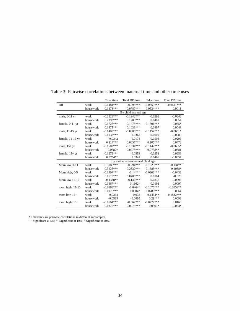
Table 3: Pairwise correlations between maternal time and other time uses
Total time Total DP time Educ time Educ DP time
All work -0.1484*** -0.098*** -0.0859*** -0.0611***housework 0.1178*** 0.0787*** 0.0534*** 0.0011
By child sex and agemale, 0-11 yr work -0.2223*** -0.1243*** -0.0298 -0.0343
housework 0.2393*** 0.1288*** 0.0489 0.0054female, 0-11 yr work -0.1726*** -0.1475*** -0.1506*** -0.065*
housework 0.1675*** 0.1039*** 0.0497 0.0043male, 11-15 yr work -0.1408*** -0.0886*** -0.1154*** -0.0601*
housework 0.1033*** 0.0362 0.0009 -0.0383female, 11-15 yr work -0.0342 -0.0174 -0.0503 -0.0295
housework 0.114*** 0.0857*** 0.105*** 0.0473male, 15+ yr work -0.1582*** -0.1034*** -0.1147*** -0.0655*
housework 0.0582* 0.0978*** 0.0738** -0.0381female, 15+ yr work -0.1272*** -0.0353 -0.0251 0.0259
housework 0.0754** 0.0341 0.0466 -0.0357By mother education and child age
Mom low, 0-11 work -0.3086*** -0.294*** -0.1623*** -0.134**housework 0.3426*** 0.2637*** 0.1685*** 0.1088*
Mom high, 0-5 work -0.1994*** -0.14*** -0.0802*** -0.0439housework 0.1619*** 0.0785*** 0.0164 -0.029
Mom low 11-15 work -0.1338** -0.146*** -0.0337 -0.0696housework 0.1667*** 0.1162* -0.0191 0.0097
mom high, 11-15 work -0.0888*** -0.0464* -0.1075*** -0.0559**housework 0.0976*** 0.0504* 0.0789*** 0.0064
mom low, 15+ work 0.0354 -0.038 -0.1454** -0.1832***housework -0.0585 -0.0895 0.21*** 0.0099
mom high, 15+ work -0.1664*** -0.0627** -0.0777*** 0.0168housework 0.0875*** 0.0973*** 0.0503* -0.054*
All statistics are pairwise correlations in different subsamples.∗∗∗ Significant at 5%;∗∗ Significant at 10%;∗ Significant at 20%.
34

Table 4: Effects of Log total maternal time
Panel A: WJ Word-Letter Identification Test Panel B: WJ Passage Comprehension TestOLS LIML Childcare Price (1) OLS LIML Childcare Price (1)
γ δ0 δa CD/N γ δ0 δa CD/N γ δ0 δa CD/N γ δ0 δa CD/NAll 0.962*** 0.21 -0.217*** 22.159*** -9.317*** 0.561*** 7.404 0.381 -2.914*** 0.062 3.508 -4.339** 0.179 7.586
[2.71] [0.28] [3.73] 1751 [3.10] [2.68] [2.01] 1731 [0.84] [2.90] [0.73] 1446 [0.74] [1.80] [0.96] 1428Mother 1.261*** -0.295 -0.174*** 18.770*** -8.309** 0.443 4.539 0.317 -1.161 -0.066 -4.608 1.359 -0.23 4.213educ≤ 12 [3.06] [0.31] [2.33] 802 [2.02] [1.78] [1.24] 789 [0.50] [0.73] [0.49] 661 [0.81] [0.42] [0.97] 648Mother 0.547 0.706 -0.262*** 23.437*** -9.426*** 0.592* 4.446 0.422 -4.382*** 0.164* 10.166** -8.763*** 0.518*** 5.594educ> 12 [0.92] [0.63] [2.99] 949 [2.49] [2.08] [1.60] 942 [0.65] [3.40] [1.51] 785 [1.78] [2.99] [ 2.18] 780Male 1.126*** 1.472* -0.322*** 26.599** -11.902* 0.718 2.237 0.501 -4.205*** 0.162* 14.629 -12.285* 0.771 2.547Child [2.34] [1.39] [3.95] 875 [1.93] [1.57] [1.22] 869 [0.87] [3.12] [1.43] 703 [1.06] [1.54] [1.28] 697Female 0.780* -1.102 -0.107 18.921*** -8.096*** 0.501** 5.935 0.266 -1.769 -0.026 0.395 -1.682 -0.02 5.148Child [1.49] [1.04] [1.28] 876 [2.43] [2.36] [1.77] 862 [0.38] [1.19] [0.21] 743 [0.07] [0.65] [0.10] 731White 0.17 2.278*** -0.365*** 19.012*** -5.637** 0.301 7.031 0.436 -1.498 -0.042 4.948 -3.591 0.133 5.722Child [0.27] [2.16] [4.49] 968 [2.73] [1.71] [1.12] 962 [0.57] [1.09] [0.37] 780 [0.91] [1.28] [0.60] 776Black 0.876*** -1.738* -0.058 15.752** -8.102** 0.405* 1.995 -0.072 -6.26*** 0.322*** 11.919 -11.085* 0.64 2.829Child [2.00] [1.58] [0.66] 635 [1.72] [1.89] [1.31] 625 [0.12] [3.99] [2.40] 538 [0.67] [1.50] [1.28] 528Male 0.458 0.91 -0.288*** 30.584*** -13.183** 0.808* 3.028 0.584 -2.72*** 0.028 2.094 -3.454 0.092 5.069Head [0.85] [0.97] [3.92] 1206 [1.99] [1.77] [1.41] 1192 [0.84] [2.21] [0.27] 996 [0.37] [1.12] [0.39] 984Female 1.034*** -0.523 -0.068 8.594*** -3.825** 0.206 9.022 -0.838* -2.604* 0.138 2.757 -3.949** 0.241* 6.998Head [2.16] [0.43] [0.73] 545 [2.60] [1.87] [1.26] 539 [1.38] [1.49] [0.97] 450 [0.72] [1.70] [1.33] 444
Panel C: WJ Applied Problems Test Panel D: WISC Digit Span TestOLS LIML Childcare Price (1) OLS LIML Childcare Price (1)
γ δ0 δa CD/N γ δ0 δa CD/N γ δ0 δa CD/N γ δ0 δa CD/NAll 0.856*** 7.749*** -0.71*** 26.533*** -3.939 0.226 7.565 -0.086 -1.934*** -0.13** 3.907 -3.72 0.011 8.075
[2.31] [9.93] [11.68] 1743 [3.27] [0.98] [0.70] 1723 [0.21] [2.16] [1.86] 1638 [0.44] [0.93] [0.03] 1618Mother 0.932*** 6.839*** -0.616*** 17.229*** -0.943 -0.024 4.937 0.026 -3.327*** -0.083 0.71 -3.787 -0.057 4.301educ≤ 12 [1.97] [6.19] [7.17] 797 [2.55] [0.26] [0.08] 784 [0.05] [2.72] [0.87] 770 [0.11] [1.20] [0.24] 757Mother 0.734 8.621*** -0.798*** 36.123*** -6.914 0.483 4.315 -0.182 -0.683 -0.178** 47.695 -20.751 1.528 4.336educ> 12 [1.25] [7.81] [9.25] 946 [2.06] [0.85] [0.73] 939 [0.27] [0.52] [1.74] 868 [0.64] [0.66] [ 0.58] 861Male 0.989** 8.772*** -0.769*** 36.094** -9.653 0.658 2.15 -0.055 -0.889 -0.163** 36.941 -19.631 1.346 2.203Child [1.91] [7.75] [8.80] 874 [1.81] [0.89] [0.78] 868 [0.10] [0.70] [1.66] 808 [0.75] [0.78] [0.66] 802Female 0.687* 6.837*** -0.658*** 20.574*** -1.028 -0.005 6.3 -0.13 -2.763*** -0.109 -1.51 -2.356 -0.145 6.816Child [1.29] [6.32] [7.75] 869 [2.80] [0.30] [0.02] 855 [0.21] [2.19] [1.10] 830 [0.27] [0.96] [0.75] 816White 0.576 9.863*** -0.855*** 26.383*** -1.005 0.049 7.074 -0.188 -2.426** -0.06 -1.045 -2.037 -0.094 6.983Child [0.92] [9.29] [10.42] 964 [3.20] [0.25] [0.15] 958 [0.27] [1.95] [0.62] 878 [0.18] [0.73] [0.42] 872Black 0.61 5.090*** -0.487*** 34.336* -9.457 0.526 2.084 -0.468 -1.354 -0.261*** -5.124 0.339 -0.384 2.488Child [1.21] [4.00] [4.84] 630 [1.30] [0.79] [0.62] 620 [0.78] [0.91] [2.24] 578 [0.42] [0.07] [1.09] 568Male 0.6 8.755*** -0.751*** 38.508*** -9.175 0.619 3.096 0.559 -2.158*** -0.092 11.004 -6.903* 0.274 2.724Head [1.12] [9.26] [10.19] 1201 [2.27] [1.10] [0.97] 1187 [0.95] [2.02] [1.09] 1145 [0.99] [1.33] [0.69] 1131Female 0.808* 5.421*** -0.632*** 8.191*** 2.072 -0.362*** 9.169 -1.483*** -0.917 -0.202* -7.141*** 1.341 -0.392*** 11.157Head [1.46] [3.85] [5.85] 542 [2.50] [0.96] [2.10] 536 [2.27] [0.55] [1.60] 493 [2.12] [0.59] [2.24] 487
Notes: (1) LIML IV is estimated childcare price and the same variable interacted with child age;Test-t are in brackets below estimated coefficients.∗∗∗ Significant at 5%;∗∗ Significant at 10%;∗ Significant at 20%.
35
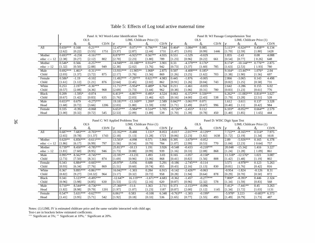
Table 5: Effects of Log total active maternal time
Panel A: WJ Word-Letter Identification Test Panel B: WJ Passage Comprehension TestOLS LIML Childcare Price (1) OLS LIML Childcare Price (1)
γ δ0 δa CD/N γ δ0 δa CD/N γ δ0 δa CD/N γ δ0 δa CD/NAll 0.650*** 0.168 -0.21*** 12.472*** -9.071*** 0.796*** 7.544 0.464* -3.084*** 0.085 5.115** -6.624*** 0.458** 6.134
[2.62] [0.22] [3.55] 1751 [3.37] [2.87] [2.44] 1731 [1.47] [3.05] [0.99] 1446 [1.70] [2.59] [1.80] 1428Mother 0.693*** -0.258 -0.161*** 8.879*** -6.925*** 0.567** 4.935 0.551 -1.529 -0.029 1.835 -2.43 0.08 4.088educ<= 12 [2.38] [0.27] [2.12] 802 [2.70] [2.23] [1.80] 789 [1.23] [0.96] [0.22] 661 [0.54] [0.77] [ 0.26] 648Mother 0.546* 0.566 -0.257*** 14.949*** -10.188*** 0.914** 3.901 0.33 -4.379*** 0.176* 8.174* -10.144*** 0.776** 2.875educ> 12 [1.32] [0.50] [2.88] 949 [2.38] [2.02] [1.76] 942 [0.73] [3.37] [1.60] 785 [1.63] [2.53] [ 1.93] 780Male 0.692*** 1.461* -0.311*** 13.931*** -11.905** 1.068* 2.875 0.507 -4.408*** 0.185* 9.164* -13.447** 1.076* 2.04Child [2.03] [1.37] [3.72] 875 [2.17] [1.76] [1.56] 869 [1.26] [3.25] [1.62] 703 [1.38] [1.90] [1.56] 697Female 0.586* -1.19 -0.102 11.492*** -7.29*** 0.621*** 4.983 0.445 -1.876 -0.005 2.866 -3.065 0.143 4.498Child [1.61] [1.12] [1.21] 876 [2.64] [2.45] [2.02] 862 [0.91] [1.26] [0.04] 743 [0.82] [1.25] [0.58] 731White 0.253 2.197*** -0.36*** 11.711*** -5.954** 0.489* 6.764 0.211 -1.461 -0.035 2.642 -3.286 0.155 6.02Child [0.57] [2.08] [4.36] 968 [2.69] [1.73] [1.44] 962 [0.38] [1.06] [0.31] 780 [0.83] [1.23] [0.61] 776Black 0.209 -1.595* -0.074 6.413** -6.807*** 0.495* 4.524 0.063 -6.372*** 0.330*** 6.262** -11.083*** 0.814*** 3.627Child [0.67] [1.42] [0.83] 635 [1.76] [2.03] [1.46] 625 [0.16] [4.00] [2.43] 538 [1.79] [3.28] [2.51] 528Male 0.653** 0.679 -0.275*** 19.181*** -13.169** 1.200* 2.589 0.842** -3.061*** 0.071 1.612 -3.611 0.137 3.328Head [1.68] [0.72] [3.66] 1206 [2.03] [1.80] [1.59] 1192 [1.71] [2.49] [0.67] 996 [0.40] [1.11] [0.42] 984Female 0.335 -0.392 -0.068 6.653*** -5.984*** 0.514** 5.705 -0.726** -2.455* 0.112 6.103* -8.052** 0.664** 2.579Head [1.00] [0.32] [0.72] 545 [2.53] [2.09] [1.89] 539 [1.70] [1.39] [0.78] 450 [1.40] [1.85] [ 1.65] 444
Panel C: WJ Applied Problems Test Panel D: WISC Digit Span TestOLS LIML Childcare Price (1) OLS LIML Childcare Price (1)
γ δ0 δa CD/N γ δ0 δa CD/N γ δ0 δa CD/N γ δ0 δa CD/NAll 0.687*** 7.683*** -0.703*** 22.352*** -9.488 1.131* 8.053 -0.017 -2.017*** -0.129** 7.722** -8.165*** 0.514* 7.975
[2.65] [9.78] [11.37] 1743 [2.18] [1.13] [1.28] 1723 [0.06] [2.23] [1.82] 1638 [1.72] [2.19] [1.34] 1618Mother 0.620** 6.856*** -0.611*** 13.503* -4.098 0.571 5.866 0.395 -3.679*** -0.052 2.89 -5.926*** 0.165 6.378educ<= 12 [1.86] [6.17] [6.99] 797 [1.56] [0.54] [0.70] 784 [1.07] [2.99] [0.53] 770 [1.04] [2.23] [ 0.64] 757Mother 0.739** 8.450*** -0.785*** 25.813** -10.13 1.191 3.926 -0.548 -0.433 -0.218*** 20.048 -15.342 1.416 3.227educ> 12 [1.81] [7.60] [8.95] 946 [1.73] [0.88] [0.99] 939 [1.16] [0.33] [2.08] 868 [1.24] [1.28] [ 1.09] 861Male 0.995*** 8.562*** -0.745*** 22.591** -13.231 1.493 3.03 0.165 -1.057 -0.158* 11.518* -12.576* 1.021 3.087Child [2.73] [7.50] [8.31] 874 [1.69] [0.96] [1.06] 868 [0.41] [0.82] [1.56] 808 [1.42] [1.48] [1.19] 802Female 0.343 6.884*** -0.665*** 20.979* -5.056 0.688 5.291 -0.186 -2.745*** -0.114 3.571 -4.978** 0.123 5.263Child [0.93] [6.34] [7.76] 869 [1.51] [0.60] [0.74] 855 [0.43] [2.16] [1.13] 830 [0.81] [1.76] [0.42] 816White 0.367 9.895*** -0.861*** 16.042*** -1.303 0.284 6.915 -0.142 -2.426** -0.063 -0.954 -1.824 -0.126 8.31Child [0.82] [9.27] [10.32] 964 [3.17] [0.32] [0.72] 958 [0.28] [1.94] [0.64] 878 [0.29] [0.70] [0.50] 872Black 0.341 5.123*** -0.495*** -12.647* 16.119*** -1.671*** 4.683 -0.362 -1.457 -0.277*** 7.800* -8.393* 0.446 2.324Child [0.96] [3.98] [4.85] 630 [1.53] [2.15] [2.16] 620 [0.87] [0.96] [2.32] 578 [1.34] [1.59] [0.83] 568Male 0.710** 8.544*** -0.736*** 27.360*** -11.6 1.363 2.711 0.373 -2.153*** -0.096 7.412* -7.441** 0.45 3.263Head [1.82] [8.98] [9.79] 1201 [1.97] [1.07] [1.23] 1187 [0.87] [2.00] [1.12] 1145 [1.34] [1.72] [1.03] 1131Female 0.547* 5.631*** -0.627*** 6.061** 0.583 -0.108 6.348 -0.763** -1.303 -0.199* -5.978* 3.223 -0.683** 6.373Head [1.41] [3.95] [5.71] 542 [1.92] [0.18] [0.33] 536 [1.65] [0.77] [1.55] 493 [1.49] [0.79] [1.73] 487
Notes: (1) LIML IV is estimated childcare price and the same variable interacted with child age;Test-t are in brackets below estimated coefficients.∗∗∗ Significant at 5%;∗∗ Significant at 10%;∗ Significant at 20%.
36

Table 6: Effects of Log educational maternal time
Panel A: WJ Word-Letter Identification Test Panel B: WJ Passage Comprehension TestOLS LIML Childcare Price (1) OLS LIML Childcare Price (1)
γ δ0 δa CD/N γ δ0 δa CD/N γ δ0 δa CD/N γ δ0 δa CD/NAll 0.344** 0.346 -0.219*** 11.991*** -10.2*** 0.879** 3.757 0.511*** -3.237*** 0.087 6.811 -9.013** 0.657* 2.723
[1.74] [0.46] [3.76] 1751 [2.56] [2.23] [1.93] 1731 [2.03] [3.20] [1.02] 1446 [1.24] [1.72] [ 1.30] 1428Mother 0.548*** -0.284 -0.155*** 8.249*** -8.997*** 0.807** 3.179 0.494 -1.532 -0.014 -0.781 -0.202 -0.144 3.581educ<= 12 [2.15] [0.29] [2.03] 802 [2.29] [2.01] [1.72] 789 [1.27] [0.97] [0.11] 661 [0.27] [0.06] [0.43] 648Mother 0.153 0.817 -0.262*** 13.241** -8.824* 0.693 1.975 0.598** -4.85*** 0.194** 9.256* -12.849*** 0.893* 1.239educ> 12 [0.51] [0.72] [3.02] 949 [1.82] [1.49] [1.25] 942 [1.80] [3.71] [1.79] 785 [1.38] [1.98] [ 1.59] 780Male 0.660*** 1.437* -0.304*** 7.000*** -4.135* 0.293 5.518 0.869*** -4.805*** 0.189** 8.179* -10.365*** 0.671** 1.784Child [2.42] [1.36] [3.77] 875 [2.73] [1.50] [1.09] 869 [2.71] [3.57] [1.69] 703 [1.53] [2.28] [ 1.72] 697Female 0.012 -0.727 -0.13* 53.6 -50.962 4.871 0.132 0.128 -1.789 -0.012 -0.323 -1.173 -0.057 1.437Child [0.04] [0.68] [1.55] 876 [0.45] [0.46] [0.44] 862 [0.33] [1.19] [0.09] 743 [0.06] [0.20] [0.09] 731White -0.296 2.573*** -0.388*** 12.641** -7.157 0.65 2.542 0.081 -1.416 -0.066 3.054 -4.13 0.209 1.82Child [1.04] [2.47] [4.83] 968 [1.65] [1.14] [1.02] 962 [0.23] [1.04] [0.58] 780 [0.68] [0.97] [ 0.51] 776Black 0.759*** -2.131** -0.027 6.713** -7.528*** 0.576* 2.42 0.810*** -6.836*** 0.381*** 16.114 -16.609 1.47 1.44Child [2.66] [1.90] [0.31] 635 [1.95] [2.15] [1.60] 625 [2.19] [4.32] [2.86] 538 [0.60] [0.93] [ 0.75] 528Male -0.056 1.168 -0.309*** 23.556 -20.199 1.872 0.834 0.048 -2.46*** 0.011 1.912 -4.279 0.198 0.756Head [0.22] [1.24] [4.22] 1206 [1.03] [0.96] [0.88] 1192 [0.15] [2.00] [0.11] 996 [0.35] [0.77] [ 0.37] 984Female 0.894*** -0.94 -0.025 5.847*** -5.642*** 0.425** 5.517 1.058*** -4.501*** 0.228* 2.405 -5.61* 0.335 4.751Head [2.72] [0.77] [0.27] 545 [2.64] [2.15] [1.83] 539 [2.47] [2.56] [1.60] 450 [0.54] [1.39] [ 0.93] 444
Panel C: WJ Applied Problems Test Panel D: WISC Digit Span TestOLS LIML Childcare Price (1) OLS LIML Childcare Price (1)
γ δ0 δa CD/N γ δ0 δa CD/N γ δ0 δa CD/N γ δ0 δa CD/NAll 0.324* 7.878*** -0.703*** 21.750** -11.445 1.285 4.229 0.206 -2.178*** -0.122** 11.430* -11.393** 0.933 4.203
[1.56] [10.02] [11.53] 1743 [1.76] [0.99] [1.10] 1723 [0.88] [2.43] [1.74] 1638 [1.44] [1.70] [ 1.23] 1618Mother 0.341 6.996*** -0.605*** 13.676* -8.19 1.067 4.09 0.363 -3.697*** -0.041 3.287 -6.799*** 0.336 4.495educ<= 12 [1.16] [6.27] [6.88] 797 [1.48] [0.76] [0.91] 784 [1.13] [3.02] [0.42] 770 [1.20] [2.21] [0.90] 757Mother 0.269 8.702*** -0.784*** 25.598 -9.601 0.992 2.014 0.084 -0.885 -0.195** 27.585 -19.558 1.741 1.473educ> 12 [0.92] [7.82] [9.17] 946 [1.19] [0.59] [0.64] 939 [0.25] [0.67] [1.91] 868 [0.72] [0.74] [0.64] 861Male 0.355 8.815*** -0.743*** 12.096*** -1.644 0.363 5.937 0.083 -0.937 -0.153* 4.932* -4.663* 0.327 4.827Child [1.21] [7.74] [8.52] 874 [2.02] [0.28] [0.61] 868 [0.26] [0.74] [1.56] 808 [1.62] [1.63] [ 1.01] 802Female 0.292 6.961*** -0.663*** 64.805 -52.098 5.264 0.182 0.344 -3.321*** -0.093 715.538 -615.281 63.719 0.474Child [1.00] [6.40] [7.76] 869 [0.44] [0.39] [0.39] 855 [1.01] [2.62] [0.93] 830 [0.02] [0.02] [ 0.02] 816White -0.235 10.281*** -0.875*** 15.873*** -2.014 0.415 2.485 0.483* -2.812*** -0.051 -6.877 2.388 -0.642* 2.892Child [0.82] [9.77] [10.77] 964 [2.02] [0.30] [0.62] 958 [1.45] [2.29] [0.53] 878 [1.19] [0.54] [1.33] 872Black 0.676*** 4.789*** -0.443*** -196.108 171.101 -19.242 3.029-0.56* -1.087 -0.279*** 6.632 -7.251 0.426 2.067Child [2.04] [3.69] [4.39] 630 [0.10] [0.10] [0.10] 620 [1.45] [0.71] [2.36] 578 [0.81] [1.00] [ 0.52] 568Male 0.065 8.974*** -0.775*** 26.575 -15.287 1.66 0.836 0.484** -2.309*** -0.105 12.931 -12.217 0.996 1.184Head [0.26] [9.51] [10.55] 1201 [1.25] [0.77] [0.84] 1187 [1.74] [2.17] [1.26] 1145 [0.83] [0.97] [ 0.72] 1131Female 0.740** 5.593*** -0.551*** 8.298*** -1.371 0.123 6.671 -0.878** -1.288 -0.177* -7.626** 4.704 -0.841*** 5.269Head [1.89] [3.88] [5.03] 542 [2.18] [0.34] [0.33] 536 [1.89] [0.76] [1.38] 493 [1.94] [1.11] [2.01] 487
Notes: (1) LIML IV is estimated childcare price and the same variable interacted with child age;Test-t are in brackets below estimated coefficients.∗∗∗ Significant at 5%;∗∗ Significant at 10%;∗ Significant at 20%.
37

Table 7: Effects of Log educational active maternal time
Panel A: WJ Word-Letter Identification Test Panel B: WJ Passage Comprehension TestOLS LIML Childcare Price (1) OLS LIML Childcare Price (1)
γ δ0 δa CD/N γ δ0 δa CD/N γ δ0 δa CD/N γ δ0 δa CD/NAll 0.302* 0.448 -0.208*** 6.702*** -5.379*** 0.431*** 17.529 0.462* -3.102*** 0.085 3.377 -5.472** 0.316 5.293
[1.31] [0.57] [3.49] 1751 [4.19] [3.01] [2.49] 1731 [1.54] [2.92] [0.98] 1446 [0.99] [1.83] [1.15] 1428Mother 0.674*** -0.225 -0.143** 6.152*** -4.877*** 0.407** 8.596 0.569 -1.174 -0.047 -1.029 -0.191 -0.145 3.864educ<= 12 [2.28] [0.22] [1.87] 802 [3.14] [2.27] [1.86] 789 [1.24] [0.71] [0.34] 661 [0.29] [0.08] [0.56] 648Mother -0.007 1.073 -0.265*** 6.924*** -5.709*** 0.436** 9.835 0.46 -4.734*** 0.201** 9.167* -13.864*** 0.971** 1.908educ> 12 [0.02] [0.90] [2.94] 949 [2.97] [2.09] [1.72] 942 [1.16] [3.43] [1.79] 785 [1.47] [2.06] [ 1.72] 780Male 0.567** 1.497* -0.295*** 4.996*** -2.678* 0.153 18.718 0.782*** -4.689*** 0.201** 4.444** -7.839*** 0.465*** 6.753Child [1.74] [1.37] [3.55] 875 [3.59] [1.49] [0.92] 869 [1.96] [3.34] [1.75] 703 [1.67] [2.95] [2.11] 697Female 0.066 -0.631 -0.115* 12.409** -11.179** 1.056** 2.726 0.165 -1.643 -0.023 -3.278 1.214 -0.308 1.276Child [0.20] [0.56] [1.35] 876 [1.86] [1.81] [1.65] 862 [0.37] [1.04] [0.18] 743 [0.48] [0.22] [0.52] 731White -0.121 2.476*** -0.379*** 6.757*** -3.382* 0.315 9.67 -0.254 -1.013 -0.079 2.148 -3.099 0.144 3.735Child [0.37] [2.28] [4.56] 968 [2.84] [1.36] [1.21] 962 [0.61] [0.71] [0.68] 780 [0.64] [0.99] [0.46] 776Black 0.496* -1.708* -0.035 3.602*** -4.912*** 0.289** 10.103 1.051*** -7.188*** 0.378*** 11.955 -14.538* 0.962* 2.19Child [1.45] [1.44] [0.39] 635 [2.38] [2.51] [1.71] 625 [2.34] [4.24] [2.75] 538 [0.95] [1.61] [1.35] 528Male 0.206 0.903 -0.283*** 7.689*** -6.008*** 0.503** 8.606 0.321 -2.672*** 0.03 1.189 -3.408 0.112 2.807Head [0.71] [0.91] [3.73] 1206 [2.94] [2.15] [1.75] 1192 [0.85] [2.06] [0.28] 996 [0.33] [1.02] [0.34] 984Female 0.228 -0.072 -0.05 3.695*** -3.279** 0.256* 12.713 0.547 -3.754*** 0.186 5.933* -7.49*** 0.490** 4.023Head [0.62] [0.06] [0.54] 545 [2.52] [1.72] [1.59] 539 [1.13] [2.07] [1.28] 450 [1.56] [2.17] [ 1.78] 444
Panel C: WJ Applied Problems Test Panel D: WISC Digit Span TestOLS LIML Childcare Price (1) OLS LIML Childcare Price (1)
γ δ0 δa CD/N γ δ0 δa CD/N γ δ0 δa CD/N γ δ0 δa CD/NAll 0.19 7.916*** -0.702*** 9.335*** -0.475 0.193 17.824 0.035 -1.958*** -0.135** 1.362 -3.204** -0.001 17.976
[0.79] [9.64] [11.22] 1743 [4.01] [0.19] [0.78] 1723 [0.13] [2.09] [1.88] 1638 [0.82] [1.82] [0.00] 1618Mother 0.244 7.119*** -0.604*** 7.621*** 0.72 0.14 10.01 0.134 -3.271*** -0.054 1.194 -4.266*** 0.058 10.775educ<= 12 [0.72] [6.19] [6.85] 797 [2.19] [0.21] [0.38] 784 [0.36] [2.59] [0.55] 770 [0.70] [2.35] [ 0.29] 757Mother 0.137 8.697*** -0.786*** 9.864*** -0.785 0.16 9.263 -0.055 -0.776 -0.208*** 2.414 -3.238 0.038 8.452educ> 12 [0.40] [7.42] [8.83] 946 [3.14] [0.22] [0.48] 939 [0.14] [0.56] [1.96] 868 [0.62] [0.78] [ 0.10] 861Male 0.271 8.829*** -0.737*** 6.353*** 3.121* -0.122 19.167 0.247 -1.068 -0.141* 1.739 -2.449 0.011 15.977Child [0.77] [7.48] [8.22] 874 [3.39] [1.36] [0.56] 868 [0.63] [0.81] [1.41] 808 [1.05] [1.21] [0.06] 802Female 0.135 6.964*** -0.662*** 15.504** -6.315 0.766 2.717 -0.135 -2.792*** -0.128 -0.19 -2.88 -0.13 4.447Child [0.41] [6.08] [7.57] 869 [1.96] [0.86] [1.00] 855 [0.35] [2.08] [1.24] 830 [0.04] [0.74] [0.30] 816White -0.127 10.274*** -0.875*** 9.649*** 1.976 0.099 9.507 0.355 -2.803*** -0.033 -1.333 -1.334 -0.206 10.6Child [0.39] [9.37] [10.43] 964 [3.42] [0.66] [0.32] 958 [0.92] [2.19] [0.33] 878 [0.65] [0.62] [0.91] 872Black 0.337 4.932*** -0.456*** 6.341 -1.129 0.107 10.77 -0.641* -0.806 -0.331*** 1.194 -2.825 -0.145 10.576Child [0.85] [3.59] [4.41] 630 [1.26] [0.21] [0.22] 620 [1.37] [0.50] [2.74] 578 [0.61] [1.12] [0.65] 568Male 0.173 8.740*** -0.762*** 10.686*** -1.096 0.317 8.349 0.351 -2.339*** -0.089 2.19 -3.934*** 0.098 9.982Head [0.59] [8.80] [10.01] 1201 [3.33] [0.32] [0.90] 1187 [1.08] [2.09] [1.04] 1145 [1.14] [1.96] [0.47] 1131Female 0.085 6.266*** -0.57*** 4.213* 2.452 -0.21 14.23 -0.883** -1.14 -0.226** -3.398* 1.206 -0.477** 11.004Head [0.20] [4.25] [5.16] 542 [1.62] [0.87] [0.83] 536 [1.69] [0.66] [1.75] 493 [1.31] [0.39] [1.68] 487
Notes: (1) LIML IV is estimated childcare price and the same variable interacted with child age;Test-t are in brackets below estimated coefficients.∗∗∗ Significant at 5%;∗∗ Significant at 10%;∗ Significant at 20%.
38

Table 8: First-Stage Estimates
First Stage Log Total Maternal TimeTotal time Directly participating time
IV A IV B x∗t−5 kt−5 kt−5at−5 R2 / N IV A IV B x∗t−5 kt−5 kt−5at−5 R2 / NAll 0.380*** -0.03*** 0.023*** 0.026* -0.001 0.069 0.873*** -0.045*** 0.090*** 0.066*** -0.006*** 0.116
[2.59] [3.75] [1.99] [1.34] [0.48] 1731 [3.80] [3.59] [4.83] [2.18] [2.05] 1731Mother 0.391* -0.038*** 0.023 0.013 0 0.067 1.294*** -0.071*** 0.092*** 0.033 -0.003 0.102educ≤ 12 [1.47] [2.56] [1.27] [0.40] [0.09] 789 [3.08] [3.00] [3.15] [0.65] [0.57] 789Mother 0.466*** -0.026*** 0.024* 0.036* -0.001 0.067 0.714*** -0.036*** 0.096*** 0.069** -0.006** 0.12educ> 12 [2.70] [2.89] [1.56] [1.50] [0.55] 942 [2.67] [2.58] [3.96] [1.87] [1.80] 942Male 0.311* -0.024*** 0.037*** 0.052** -0.003 0.076 0.722*** -0.043*** 0.099*** 0.104*** -0.01*** 0.138Child [1.47] [2.08] [2.19] [1.90] [1.08] 869 [2.19] [2.35] [3.70] [2.43] [2.36] 869Female 0.455*** -0.037*** 0.01 -0.002 0.001 0.064 1.005*** -0.048*** 0.087*** 0.024 -0.002 0.086Child [2.23] [3.32] [0.63] [0.06] [0.48] 862 [3.14] [2.78] [3.30] [0.58] [0.45] 862White 0.276** -0.028*** 0.034** 0.014 -0.001 0.078 0.407* -0.045*** 0.045* 0.028 -0.004* 0.111Child [1.69] [3.43] [1.93] [0.68] [0.32] 962 [1.52] [3.30] [1.57] [0.81] [1.31] 962Black 0.478* -0.035*** 0 0.012 0.001 0.042 1.342*** -0.045* 0.097*** 0.090* -0.007 0.093Child [1.47] [1.96] [0.02] [0.28] [0.32] 625 [2.70] [1.62] [3.01] [1.40] [1.10] 625Male 0.186 -0.018*** 0.037*** 0.048*** -0.003* 0.085 0.389* -0.028*** 0.079*** 0.078*** -0.008*** 0.121Head [1.18] [2.27] [1.99] [2.32] [1.58] 1192 [1.59] [2.26] [2.90] [2.44] [2.81] 1192Female 0.656** -0.075*** -0.039** -0.056 0.007* 0.064 1.817*** -0.11*** 0.052* -0.027 0.004 0.094Head [1.76] [3.59] [1.66] [1.28] [1.64] 539 [3.09] [3.34] [1.36] [0.39] [0.58] 539
First Stage Log Educational Maternal TimeTotal time Directly participating time
IV A IV B x∗t−5 kt−5 kt−5at−5 R2 / N IV A IV B x∗t−5 kt−5 kt−5at−5 R2 / NAll 0.871*** -0.048*** 0.104*** 0.076** -0.007* 0.078 1.470*** -0.093*** 0.034* -0.001 0 0.098
[2.58] [2.65] [4.05] [1.74] [1.61] 1731 [5.02] [5.91] [1.37] [0.02] [0.06] 1731Mother 1.260*** -0.075*** 0.144*** 0.066 -0.007 0.1 1.774*** -0.105*** 0.090*** -0.023 0.001 0.109educ≤ 2 [2.35] [2.50] [3.79] [1.02] [1.17] 789 [3.87] [4.11] [2.51] [0.42] [0.25] 789Mother 0.861** -0.043** 0.069*** 0.058 -0.004 0.04 1.381*** -0.091*** -0.008 0.004 0.001 0.09educ> 12 [1.90] [1.84] [1.97] [0.94] [0.63] 942 [3.46] [4.43] [0.24] [0.07] [0.11] 942Male 1.512*** -0.081*** 0.130*** 0.013 0.001 0.088 2.199*** -0.133*** 0.003 -0.055 0.007* 0.129Child [3.19] [3.14] [3.62] [0.21] [0.09] 869 [5.43] [6.06] [0.08] [1.06] [1.43] 869Female 0.188 -0.013 0.073*** 0.147*** -0.014*** 0.068 0.697* -0.052*** 0.067** 0.053 -0.007 0.076Child [0.39] [0.51] [2.01] [2.32] [2.43] 862 [1.64] [2.29] [1.85] [0.93] [1.26] 862White 0.09 -0.036* 0.060** 0.039 -0.007 0.064 0.604* -0.076*** 0.001 -0.015 -0.004 0.104Child [0.20] [1.59] [1.72] [0.67] [1.28] 962 [1.51] [3.80] [0.03] [0.29] [0.75] 962Black 1.375*** -0.07*** 0.130*** 0.031 -0.003 0.078 2.359*** -0.128*** 0.049 -0.044 0.008 0.104Child [2.19] [2.00] [2.92] [0.38] [0.38] 625 [4.39] [4.30] [1.13] [0.63] [1.16] 625Male 0.191 -0.023 0.114*** 0.105*** -0.011*** 0.074 0.817*** -0.071*** 0.029 0.024 -0.005 0.1Head [0.47] [1.12] [3.69] [2.01] [2.34] 1192 [2.33] [3.97] [0.98] [0.52] [1.18] 1192Female 1.896*** -0.132*** -0.014 -0.051 0.007 0.084 2.966*** -0.17*** 0.028 -0.119* 0.016*** 0.108Head [2.66] [3.29] [0.27] [0.60] [0.87] 539 [4.80] [4.95] [0.59] [1.63] [2.19] 539
Notes:IV A is estimated childcare price; (2)IV B is the estimated childcare price and child age interactionReported values are estimated using the sample of valid WJ Letter-Word Identification Test, which is the largest one among all the cognitive tests considered in this paper. First-stage estimations forsamples with valid Applied Problems, Passage Comprehension, and Digit Span tests are very similar, but differ because there are missing values for some tests in the CDS sample.Test-t are in brackets below estimated coefficients.∗∗∗ Significant at 5%;∗∗ Significant at 10%;∗ Significant at 20%.
39

this approach is not directly applicable to the problem in here because we are using panel data.
We implement the two-stage Wooldridge (1995) estimator forpanel data selection model due to its
robustness and computational easiness.
To generate a sound identification strategy, we came up with variables that affect the exten-
sive margin of childcare use (i.e whether or not they decide to use childcare services), but not
the intensive margin (i.e how many hours of childcare to buy once the household decides to use
this service). Following?) we assert that variables such as the presence of husband, number of
adults aged 18 to 70; number of other older children aged 14-17, the average welfare income and
the average child subsidies in the year and the state in whichthe household is located affect the
extensive but not the intensive margin of childcare demand.Other specifications were also tried
(with state dummies trying to capture other welfare incentives mothers may face), but the results
remain roughly unaltered. In the main equation, we considerthe following regressors: log of the
per capita family income, log of the house value, mother age,and mother schooling. We believe
that the childcare price faced by individuals may depend on these variables. More affluent fami-
lies live in wealthier neighborhoods in which these services are more expensive. Mother age and
education may influence the kind of jobs they have and indirectly affect the price of childcare they
face in the nearby area.
Using these estimates, we construct expected offered childcare prices depending of household
income, maternal characteristics, and state welfare policies.
Appendix 3 Construction of Home Quality Index
The CDS interviewer is asked several questions regarding the household he/she visits. In all of
these questions the interviewer has to express his/her agreement with the following statements
• Interior of the home is dark or perceptually monotonous.
• All visible rooms in the (house/apartment) are cluttered
40

• All visible rooms in the (house/apartment) are clean
• Child’s play environment is safe (no potentially dangeroushealth or structural hazards within
a child’s range)
Answers are expressed using a Likert scale ranging from 1 to 5( “Not at all” (1) to “Somewhat”
(3) to “Very much” (5)) except for the last one which receivesa value of 5 if the interviewer agrees
or 1 if he/she does not agree or does not know. Since we want theHome Quality Index to be a
positive scale we reverse the scale of the two first questions. Once this is done, the Home Quality
Index is built by adding the scores for the four mentioned questions. Although the measure cannot
completely capture the quality of the goods and the environment where the child lives, it is a
consistent measure we can compute from the three waves of theCDS.
References
Aguiar, M. and E. Hurst (2007). Measuring Trends in Leisure:The Allocation of Time Over
Five Decades.The Quarterly Journal of Economics 122(3), 969–1006.
Almond, D. and J. Currie (2010, March). Human Capital Development Before Age Five. Work-
ing Paper 15827, National Bureau of Economic Research.
Angrist, J. D. and J.-S. Pischke (2009).Mostly Harmless Econometrics - An Empiricist Com-
panion. Princeton University Press.
Bernal, R. (2008, November). The Effect Of Maternal Employment and Child Care on Chil-
dren’s Cognitive Development.International Economic Review 49(4), 1173–1209.
Bernal, R. and M. P. Keane (2008). Child Care Choices and Children’s Cognitive Achievement:
The Case of Single Mothers. Mimeo.
Bernal, R. and M. P. Keane (2010). Quasi-structural estimation of a model of childcare choices
and child cognitive ability production.Journal of Econometrics 156(1), 164 – 189. Struc-
tural Models of Optimization Behavior in Labor, Aging, and Health.
41

Bianchi, S. (2000). Maternal employment and time with children: Dramatic change or surpris-
ing continuity?Demography 37(4), 401–414.
Blau, D. M. (1999, May). The effect of income on child development.The Review of Economics
and Statistics 81(2), 261–276.
Blau, F. D. and A. J. Grossberg (1992, August). Maternal Labor Supply and Children’s Cogni-
tive Development.The Review of Economics and Statistics 74(3), 474–81.
Bound, J., D. A. Jaeger, and R. M. Baker (1995, Jun). ProblemsWith Instrumental Variables
Estimation When the Correlation Between the Instruments and the Endogenous Explana-
tory Variable is Weak.Journal of the American Statistical Association 90(430), 443–450.
Application and Case Studies.
Brooks-Gunn, J., W. Han, and J. Waldfogel (2002). Maternal Employment and Child Cognitive
Outcomes in the First Three Years of Life: The NICHD Study of Early Child Care.Child
Development 73(4), 1052–1072.
Bryant, W. K. and C. D. Zick (1996, Feb). An Examination of Parent-Child Shared Time.Jour-
nal of Marriage and the Family 58, 227–237.
Burton, P., S. Phipps, and L. Curtis (2002, May). All in the Family: A Simultaneous Model of
Parenting Style and Child Conduct.American Economic Review 92(2), 368–372.
Carneiro, P. and M. Rodrigues (2009). Evaluating the Effectof Maternal Time on Child Devel-
opment Using the Generalized Propensity Score. Institute for the Study of Labor, 12th IZA
European Summer School in Labor Economics.
Cawley, J. and F. Liu (2007, November). Mechanisms for the Association Between Maternal
Employment and Child Cognitive Development. Working Paper13609, National Bureau of
Economic Research.
Connelly, R. and J. Kimmel (2003). The Effect of Child Care Costs on the Employment and
Welfare Recipiency of Single Mothers.Southern Economic Journal, 498–519.
42

Cragg, J. G. and S. G. Donald (1993, April). Testing Identifiability and Specification in Instru-
mental Variable Models.Econometric Theory 9(02), 222–240.
Craig, L. (2006). Parental Education, Time in Paid Work and Time with Children: an Australian
Time-diary Analysis.The British Journal of Sociology 57(4), 553–575.
Cunha, F. and J. Heckman (2007, May). The Technology of SkillFormation.American Eco-
nomic Review 97(2), 31–47.
Cunha, F. and J. J. Heckman (2008). Formulating, Identifying and Estimating the Technology
of Cognitive and Noncognitive Skill Formation.Journal of Human Resources 43(4), 738 –
782.
Currie, J., M. Stabile, P. Manivong, and L. L. Roos (2008, November). Child Health and Young
Adult Outcomes. NBER Working Papers 14482, National Bureauof Economic Research,
Inc.
Danziger, S. and J. Waldfogel (2000).Securing the Future: Investing in Children from Birth
to College. The Ford Foundation Series on Asset Building. New York, NY:Russel Sage
Foundation.
Datcher-Loury, L. (1988, Aug). Effects of Mother’s Home Time on Children’s Schooling.The
Review of Economics and Statistics 70(3), 367–373.
Del Boca, D., C. Flinn, and M. Wiswall (2010, August). Household Choices and Child Devel-
opment. IZA Discussion Papers 5155, Institute for the Studyof Labor (IZA).
Dooley, M. and J. Stewart (2007). Family Income, Parenting Styles and Child Behavioural-
Emotional Outcomes.Health Economics 16(2), 145–162.
Folbre, N., J. Yoon, K. Finnoff, and A. S. Fuligni (2005). By What Measure? Family Time
Devoted to Children in the United States.Demography 42(2), 373–390.
Gauthier, A. H., T. M. Smeeding, and F. F. Furstenberg (2004). Are Parents Investing Less
Time in Children? Trends in Selected Industrialized Countries.Population and Development
43

Review 30(4), 647–671.
Gronau, R. (1977). Leisure, Home production, and Work: the Theory of the Allocation of Time
Revisited.The Journal of Political Economy 85(6), 1099–1123.
Guryan, J., E. Hurst, and M. Kearney (2008). Parental education and parental time with children.
Journal of Economic Perspectives 22(3), 23–46.
Heckman, J. J. (1976). The Common Structure of Statistical Models of Truncation, Sample
Selection and Limited Dependent Variables and a Simple Estimator for such Models.Annals
of Economic and Social Measurement 5, 475–92.
Heckman, J. J., J. Stixrud, and S. Urzúa (2006). The Effects of Cognitive and Noncogni-
tive Abilities on Labor Market Outcomes and Social Behavior. Journal of Labor Eco-
nomics 24(3), 411–482.
Herbst, C. M. and E. Tekin (2010). Child care subsidies and child development.Economics of
Education Review 29(4), 618 – 638.
Hill, C. R. and F. P. Stafford (1985).Parental Care of Children: Time Diary Estimates of Quan-
tity, Predictability and Variety, Chapter 17, pp. 415–438. Time, Goods, and Well-Being.
Survey Research Center, Institute for Social Research, TheUniversity of Michigan.
Hill, M. A. and J. O’Neill (1994). Family Endowments and the Achievement of Young Children
with Special Reference to the Underclass.Journal of Human Resources 29(4), 1064–1100.
Hofferth, S. L. (1999). Family Reading to Young Children: Social Desirability and Cultural
Biases in Reporting. InWorkshop on Measurement of and Research on Time Use, Committee
on National Statistics. National Research Council.
Hsin, A. (2008). Mothers’ Time with Children and the Social Reproduction of Cognitive Skills.
unpublished manuscript, California Center for PopulationResearch, University of Califor-
nia, Los Angeles.
Hsin, A. (2009). Parent’s Time with Children: Does Time Matter for Children’s Cognitive
44

Achievement?Social Indicator Research: Special Edition on Time Use (John Robinson,
ed.) 93, 123–126.
Imbens, G. W. and J. D. Angrist (1994). Identification and Estimation of Local Average Treat-
ment Effects.Econometrica 62(2), pp. 467–475.
James-Burdumy, S. (2005). The Effect of Maternal Labor Force Participation on Child Devel-
opment.Journal of Labor Economics 23(1), 177–211.
Juster, F. and F. Stafford (1991). The Allocation of Time: Empirical Findings, Behavioral Mod-
els, and Problems of Measurement.Journal of Economic Literature 29(2), 471–522.
Juster, F. T. (1985).Conceptual and Methodological Issues Involved in the Measurement of Time
Use, Chapter 2, pp. 19–32. Time, Goods, and Well-Being. Survey Research Center, Institute
for Social Research, The University of Michigan.
Kimmel, J. and R. Connelly (2007). Mothers’ Time Choices Caregiving, Leisure, Home Pro-
duction, and Paid Work.Journal of Human Resources 42(3), 643–681.
Monna, B. and A. Gauthier (2008). A Review of the Literature on the Social and Economic
Determinants of Parental Time.Journal of Family and Economic Issues 29(4), 634–653.
Murray, M. P. (2006, Fall). Avoiding Invalid Instruments and Coping with Weak Instruments.
Journal of Economic Perspectives 20(4), 111–132.
Neidell, M. J. (2000, November). Early Parental Time Investments In Children’s Human Cap-
ital Development: Effects Of Time In The First Year On Cognitive And Non-Cognitive
Outcomes. UCLA Economics Working Papers 806, UCLA Department of Economics.
Robinson, J. P. (1985).The Validity and Reliability of Diaries versus AlternativeTime Use
Measures, Chapter 3, pp. 33–62. Time, Goods, and Well-Being. Survey Research Center,
Institute for Social Research, The University of Michigan.
Ruhm, C. (2004). Parental Employment and Child Cognitive Development.Journal of Human
Resources 39(1), 155.
45

Sandberg, J. L. and S. L. Hofferth (2001). Changes in Children’s Time with Parents: United
States, 1981-1997.Demography 38(3), 423–436.
Shea, J. (2000). Does Parents’ Money Matter?Journal of Public Economics 77, 155–184.
Stock, J., J. Wright, and M. Yogo (2002, Oct). A Survey of WeakInstruments and Weak Identi-
fication in GMM.Journal of Business and Economic Statistics 20(4), 518–529.
Stock, J. H. and M. Yogo (2005).Testing for Weak Instruments in Linear IV Regression, Chapter
Identification and Inference for Econometric Models: Essays in Honor of Thomas Rothen-
berg, pp. 80–108. Cambridge University Press.
Todd, P. E. and K. I. Wolpin (2003). On the Specification and Estimation of the Production
Function for Cognitive Achievement.The Economic Journal 113(485), F3–F33.
Waldfogel, J., W. Han, and J. Brooks-Gunn (2002). The Effects of Early Maternal Employment
on Child Cognitive Development.Demography 39(2), 369–392.
Wechsler, D. (1974).Manual for the Wechsler Intelligence Scale for Children, Revised. New
York: Psychological Corp.
Woodcock, R., M. Johnson, and N. Mather (1989).Woodcock-Johnson tests of achievement:
standard and supplemental batteries. DLM Teaching Resources.
Wooldridge, J. M. (1995, July). Selection Corrections for Panel Data Models under Conditional
Mean Independence Assumptions.Journal of Econometrics 68(1), 115–132.
Wooldridge, J. M. (2002).Econometric Analysis of Cross Section and Panel Data. The MIT
Press.
Yeung, W.-J., J. F. Sandberg, P. E. Davis-Kean, and S. L. Hofferth (2001). Children’s Time with
Fathers in Intact Families.Journal of Marriage and the Family 63(1), 136–154.
Zick, C., W. Bryant, and E. Österbacka (2001). Mothers’ employment, parental involvement,
and the implications for intermediate child outcomes.Social Science Research 30(1), 25–49.
46