categorical data analysis - pcu teaching...
TRANSCRIPT

Categorical Data Analysis
References : Alan Agresti, Categorical Data Analysis, Wiley Interscience, New Jersey, 2002
Bhattacharya, G.K., Johnson, R.A., Statistical Concepts and Methods, Wiley,1977
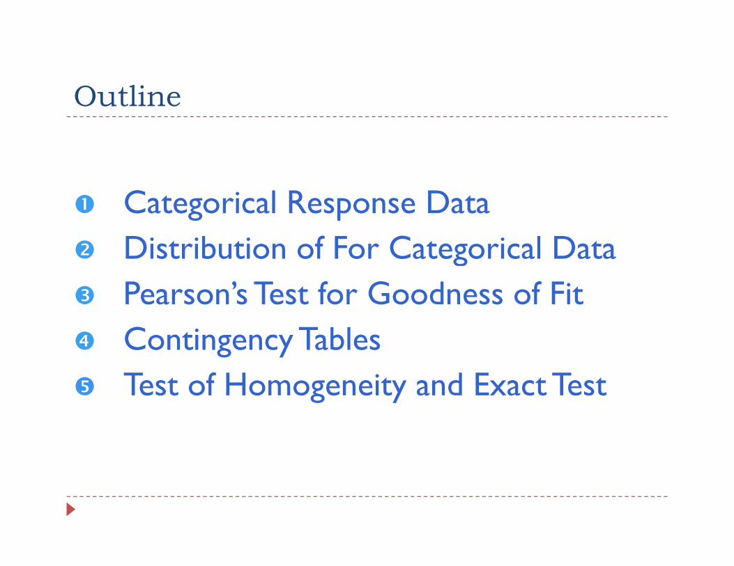
OutlineOutline
Categorical Response DataDistribution of For Categorical Data Distribution of For Categorical Data Pearson’s Test for Goodness of FitContingency TablesTest of Homogeneity and Exact TestTest of Homogeneity and Exact Test
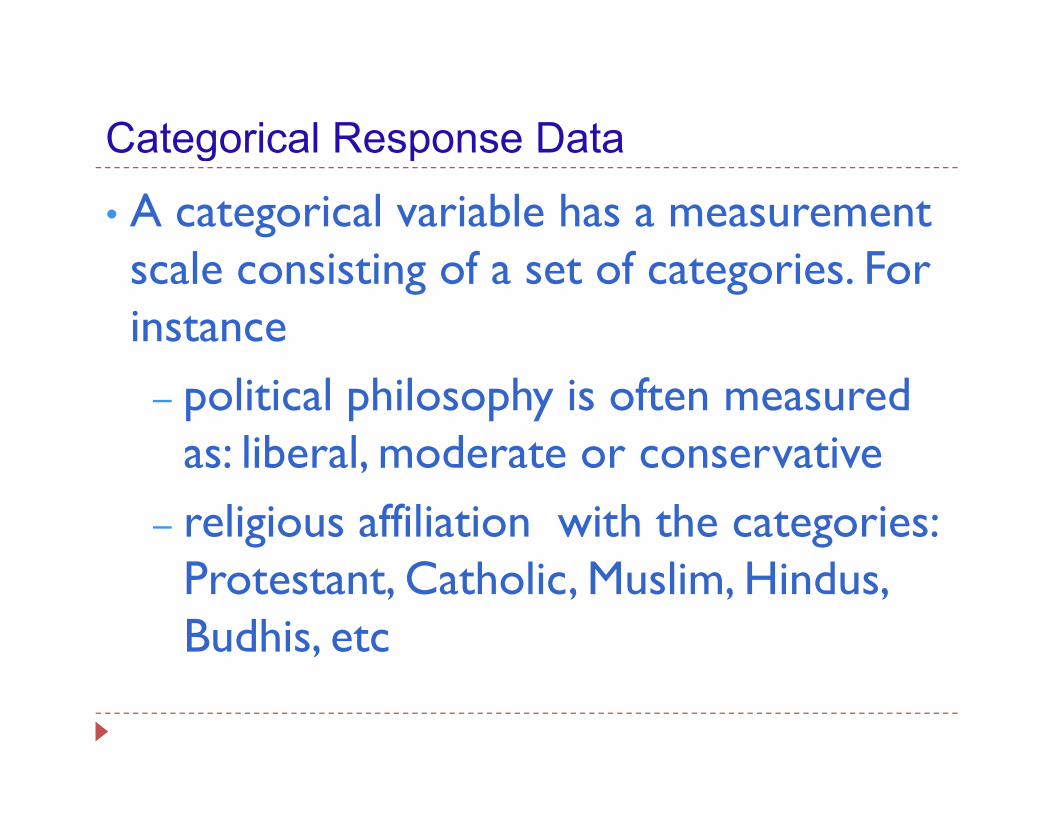
Categorical Response DataCategorical Response Data
• A categorical variable has a measurement l f f F scale consisting of a set of categories. For
instance– political philosophy is often measured
as: liberal moderate or conservativeas: liberal, moderate or conservative– religious affiliation with the categories:
Protestant, Catholic, Muslim, Hindus, Budhis, etc
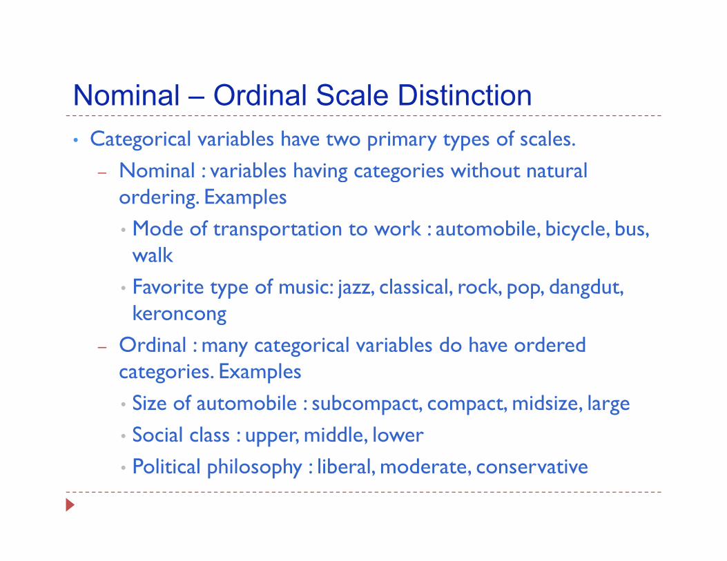
Nominal – Ordinal Scale DistinctionNominal Ordinal Scale Distinction• Categorical variables have two primary types of scales.
– Nominal : variables having categories without natural Nominal : variables having categories without natural ordering. Examples• Mode of transportation to work : automobile, bicycle, bus, walk
• Favorite type of music: jazz, classical, rock, pop, dangdut, keroncongkeroncong
– Ordinal : many categorical variables do have ordered categories. Examples• Size of automobile : subcompact, compact, midsize, large• Social class : upper, middle, lower• Political philosophy : liberal, moderate, conservative
Nominal – Ordinal Scale DistinctionNominal Ordinal Scale Distinction
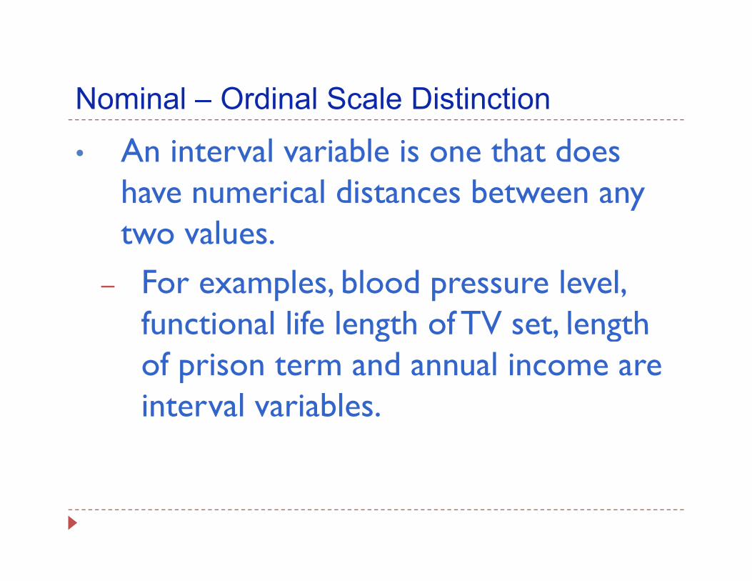
• An interval variable is one that does h l d b have numerical distances between any two values.
– For examples, blood pressure level, functional life length of TV set length functional life length of TV set, length of prison term and annual income are i t l i bl interval variables.
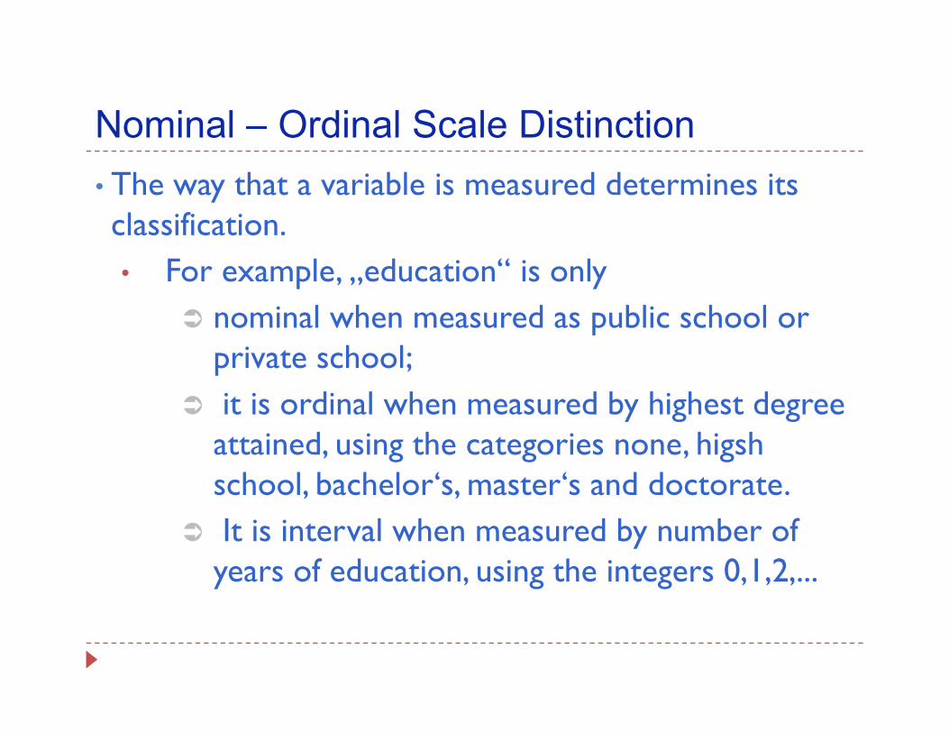
Nominal – Ordinal Scale DistinctionNominal Ordinal Scale Distinction• The way that a variable is measured determines its classificationclassification.• For example, „education“ is only
nominal when measured as public school or nominal when measured as public school or private school;it is ordinal when measured by highest degree it is ordinal when measured by highest degree attained, using the categories none, higsh school, bachelor‘s, master‘s and doctorate. It is interval when measured by number of years of education, using the integers 0,1,2,...
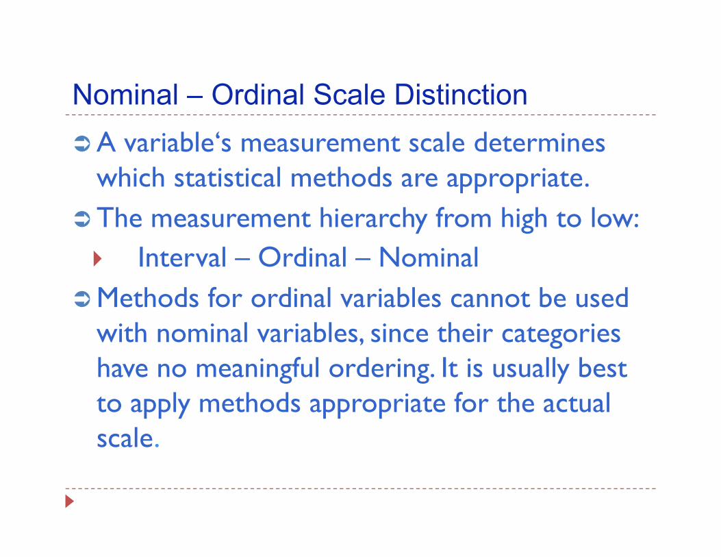
Nominal – Ordinal Scale DistinctionNominal Ordinal Scale DistinctionA variable‘s measurement scale determines
hich statistical meth ds are a r riatewhich statistical methods are appropriate.The measurement hierarchy from high to low:
Interval – Ordinal – NominalMethods for ordinal variables cannot be used with nominal variables, since their categories have no meaningful ordering. It is usually best to apply methods appropriate for the actual scale.
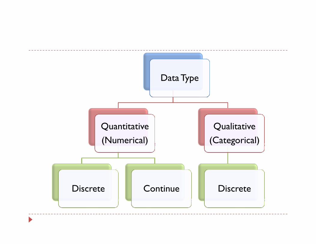
D t TData Type
Quantitative(N i l)
Qualitative(C i l)(Numerical) (Categorical)
Discrete Continue Discrete
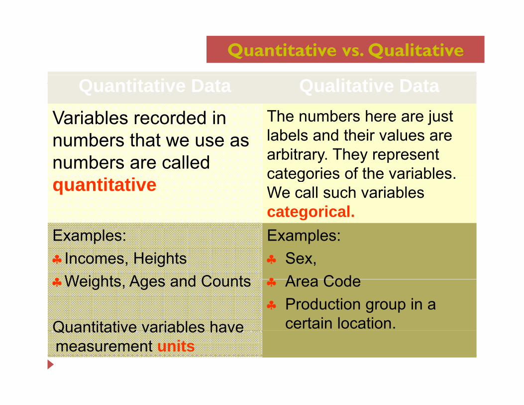
Quantitative vs. Qualitative
Quantitative Data Qualitative DataVariables recorded in The numbers here are just numbers that we use as numbers are called
labels and their values are arbitrary. They represent categories of the variablesquantitative categories of the variables. We call such variablescategorical.
Examples:♣Incomes, Heights♣Weights Ages and Counts
Examples:♣ Sex, ♣ Area Code♣Weights, Ages and Counts
Quantitative variables have
♣ Area Code♣ Production group in a
certain location.Quantitative variables have measurement units
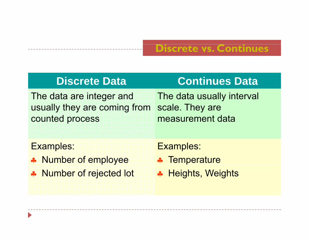
Discrete vs. Continues
Discrete Data Continues DataThe data are integer and
ll th i fThe data usually interval
l Thusually they are coming from counted process
scale. They are measurement data
Examples:♣ Number of employee
Examples:♣ Temperaturey
♣ Number of rejected lot ♣ Heights, Weights
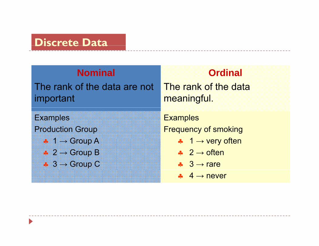
Discrete DataDiscrete Data
Nominal OrdinalThe rank of the data are not important
The rank of the data meaningful.
ExamplesProduction Group
1 G A
ExamplesFrequency of smoking
1 ft♣ 1 → Group A♣ 2 → Group B♣ 3 → Group C
♣ 1 → very often♣ 2 → often♣ 3 → rare♣ 4 → never
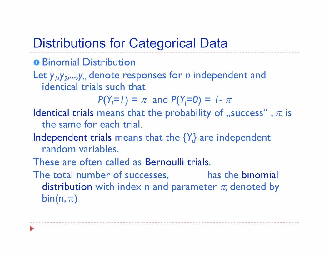
Distributions for Categorical DataDistributions for Categorical DataBinomial Distribution
Let y1,y2,...,yn denote responses for n independent and y1,y2, ,yn p pidentical trials such that
P(Yi=1) = π and P(Yi=0) = 1- πId ti l t i l th t th b bilit f “ i Identical trials means that the probability of „success“ , π, is
the same for each trial.Independent trials means that the {Yi} are independent p i p
random variables.These are often called as Bernoulli trials. The total number of successes has the binomial The total number of successes, has the binomial
distribution with index n and parameter π, denoted by bin(n, π)
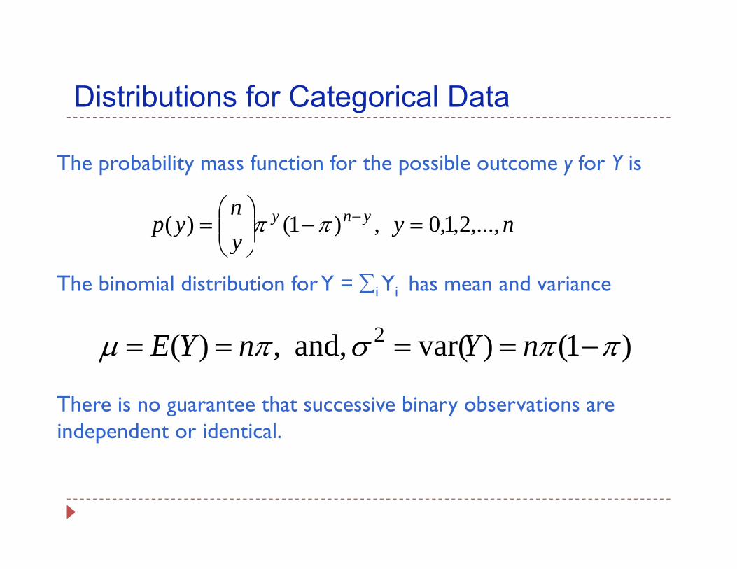
Distributions for Categorical DataDistributions for Categorical Data
The probability mass function for the possible outcome y for Y is
nyyn
yp yny ,...,2,1,0,)1()( =−⎟⎟⎠
⎞⎜⎜⎝
⎛= −ππ
The binomial distribution for Y = ∑i Yi has mean and variance
y ⎠⎝
)1()var(and,,)( 2 ππσπμ −==== nYnYE
There is no guarantee that successive binary observations are independent or identical.
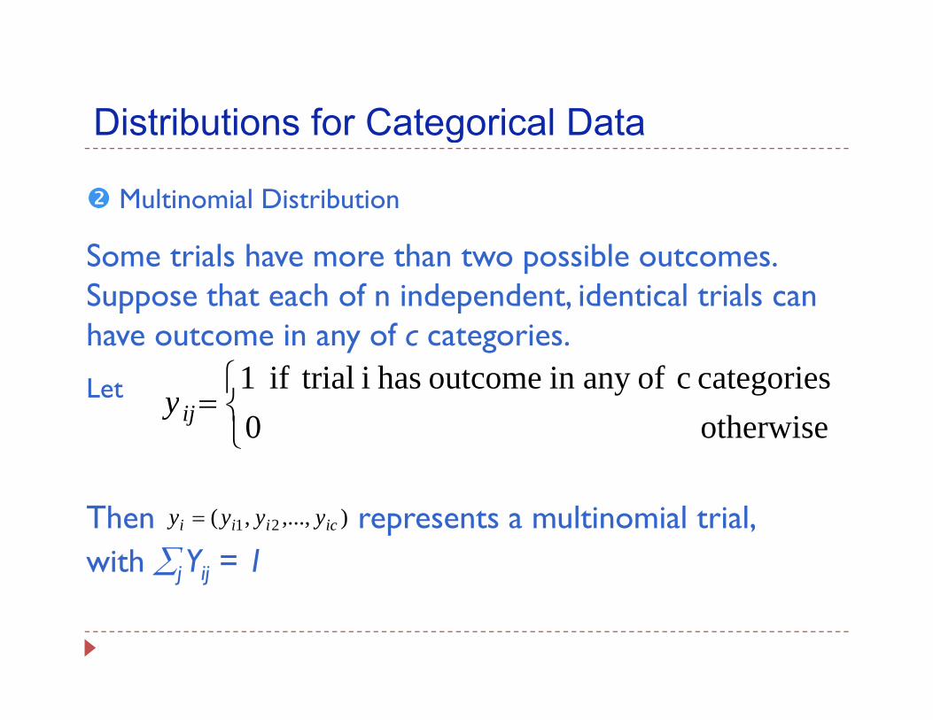
Distributions for Categorical DataDistributions for Categorical Data
Multinomial Distribution
Some trials have more than two possible outcomes. Suppose that each of n independent, identical trials can have outcome in any of c categories.
Let⎨⎧
=categories c ofany in outcome has i trialif1
y⎩⎨=
otherwise0ijy
Then represents a multinomial trial, with ∑j Yij = 1
),...,,( 21 iciii yyyy =
Distributions for Categorical DataDistributions for Categorical Data
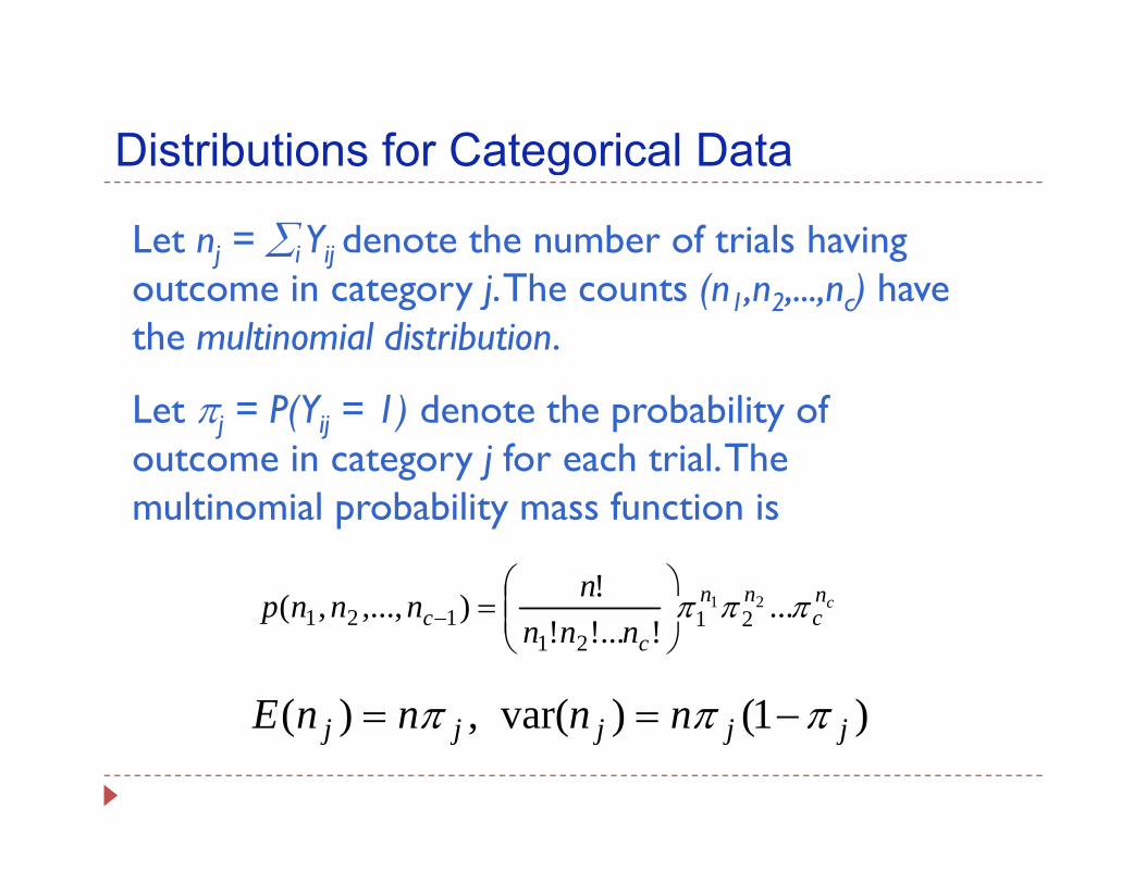
Let nj = ∑i Yij denote the number of trials having Th ( ) h outcome in category j. The counts (n1,n2,...,nc) have
the multinomial distribution.
Let πj = P(Yij = 1) denote the probability of outcome in category j for each trial. The
lti i l b bilit f ti i multinomial probability mass function is
cnnnnnnnp πππ!)( 21⎟⎟⎞
⎜⎜⎛
= cc
c nnnnnnp πππ ...
!!...!),...,,( 21
21121 ⎟⎟
⎠⎜⎜⎝
=−
)1()var()( jjjjj nnnnE πππ −== )1()var(,)( jjjjj nnnnE πππ ==
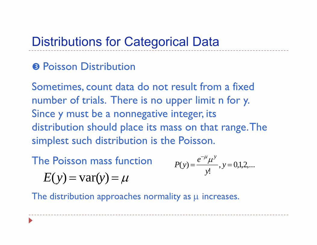
Distributions for Categorical DataDistributions for Categorical Data
Poisson Distribution
Sometimes, count data do not result from a fixed number of trials. There is no upper limit n for y. Since y must be a nonnegative integer, its distribution should place its mass on that range. The i l t h di t ib ti i th P isimplest such distribution is the Poisson.
The Poisson mass function ,...2,1,0,!
)( ==−
yeyPyμμ
The distribution approaches normality as μ increases.
!yμ== )var()( yyEpp y μ
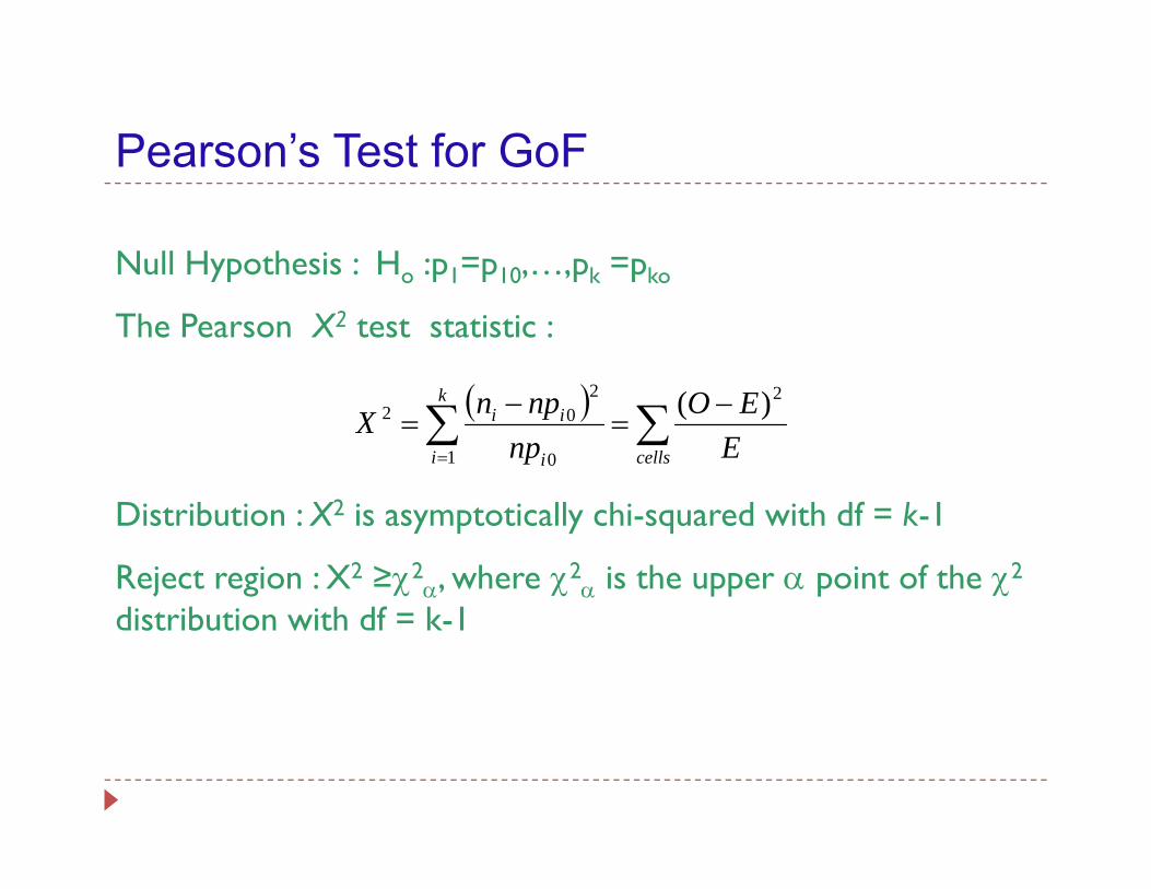
Pearson’s Test for GoFPearson s Test for GoF
Null Hypothesis : Ho :p1=p10,…,pk =pkoyp o p1 p10, ,pk pko
The Pearson X2 test statistic :
( )k 22
2
( )∑ ∑=
−=
−=
k
i cellsi
ii
EEO
npnpnX
1
2
0
202 )(
Distribution : X2 is asymptotically chi-squared with df = k-1
Reject region : X2 ≥χ2α, where χ2
α is the upper α point of the χ2
di t ib ti ith df = k 1distribution with df = k-1
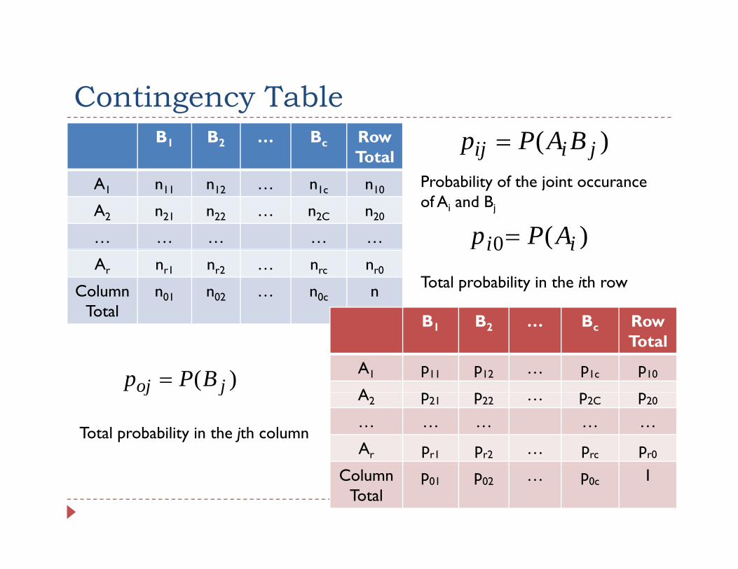
Contingency TableContingency TableB1 B2 … Bc Row
TotalP b bili f h j i
)( jiij BAPp =A1 n11 n12 … n1c n10
A2 n21 n22 … n2C n20
… … … … …
Probability of the joint occuranceof Ai and Bj
)(0 ii APp =Ar nr1 nr2 … nrc nr0
Column Total
n01 n02 … n0c n
B B B Row
)(0 iip
Total probability in the ith row
B1 B2 … Bc Row Total
A1 p11 p12 … p1c p10
A)( joj BPp =
A2 p21 p22 … p2C p20
… … … … …
Ar pr1 pr2 … prc pr0
jj
Total probability in the jth column
Column Total
p01 p02 … p0c 1
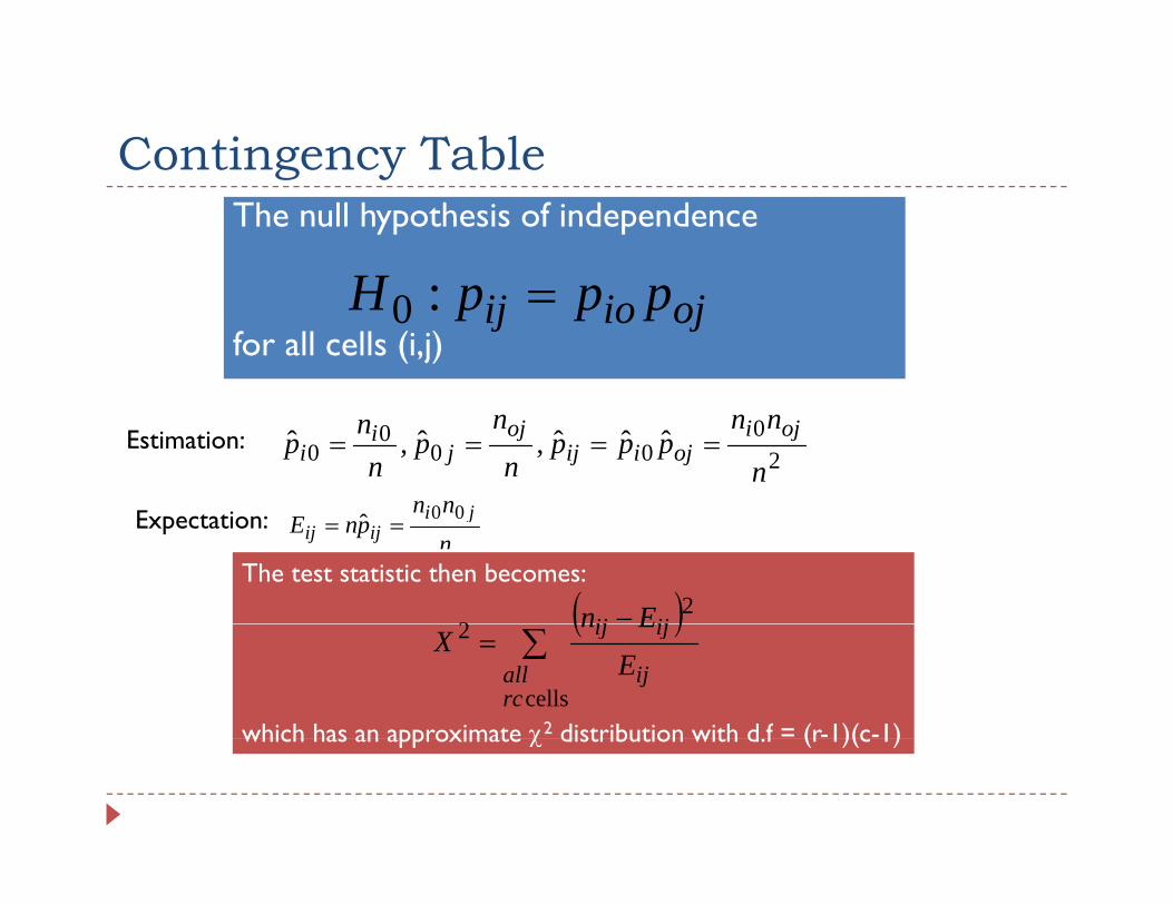
Contingency TableContingency TableThe null hypothesis of independence
Hfor all cells (i,j)
ojioij pppH =:0
Estimation:2
000
00 ˆˆˆ,ˆ,ˆ
n
nnppp
nn
pn
np oji
ojiijoj
ji
i ====
nn ji 00Expectation:nnn
pnE jiijij
00ˆ ==
The test statistic then becomes:
( )− 22 ijij En
which has an approximate χ2 distribution with d f = (r-1)(c-1)
( )∑=
cells
2
rcall ij
ijij
EEn
X
which has an approximate χ distribution with d.f (r 1)(c 1)
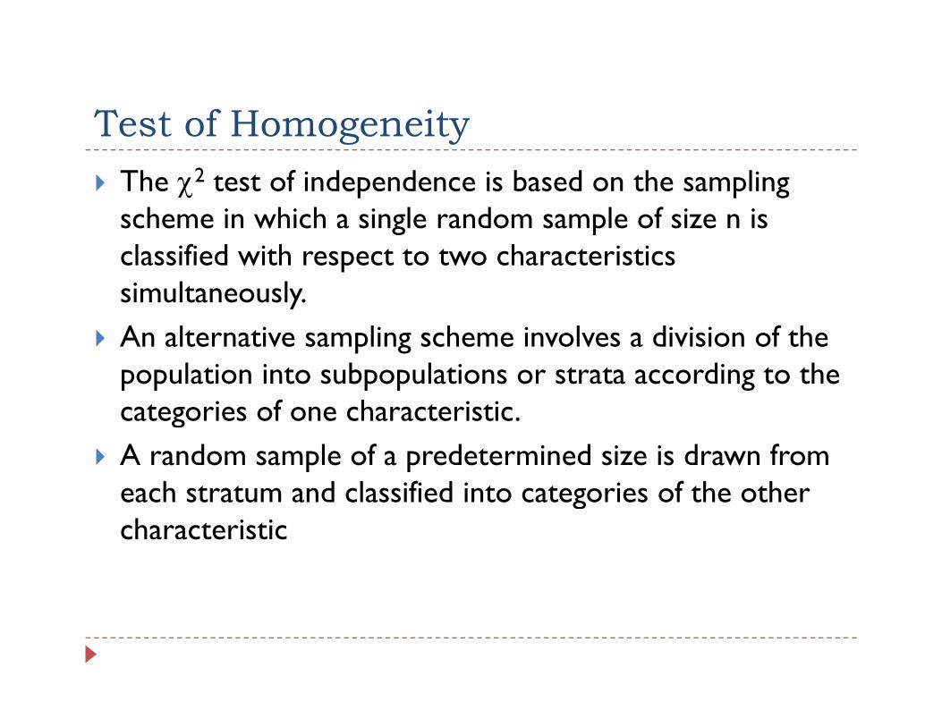
Test of HomogeneityTest of HomogeneityThe χ2 test of independence is based on the sampling scheme in which a single random sample of size n is scheme in which a single random sample of size n is classified with respect to two characteristics simultaneously.An alternative sampling scheme involves a division of the population into subpopulations or strata according to the categories of one characteristiccategories of one characteristic.A random sample of a predetermined size is drawn from each stratum and classified into categories of the other each stratum and classified into categories of the other characteristic
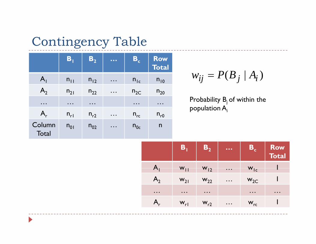
Contingency TableContingency TableB1 B2 … Bc Row
Total)|( ijij ABPw =A1 n11 n12 … n1c n10
A2 n21 n22 … n2C n20
… … … … … Probability Bj of within the l ti A
)|( ijij ABPw =
Ar nr1 nr2 … nrc nr0
Column Total
n01 n02 … n0c n
population Ai
B1 B2 … Bc Row Total
A w w 2 w 1A1 w11 w12 … w1c 1
A2 w21 w22 … w2C 1
… … … … …
Ar wr1 wr2 … wrc 1
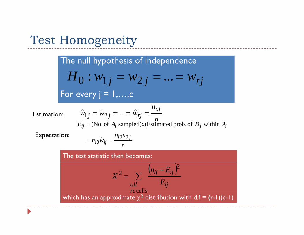
Test HomogeneityTest HomogeneityThe null hypothesis of independence
HFor every j = 1,…,c
rjjj wwwH === ...: 210
Estimation: nn
www ojrjjj ==== ˆ...ˆˆ 21
ABAE ijiij within of prob. Estimatedsampled)x( of (No. =
Expectation:nnn
wn jiiji
000 ˆ ==
The test statistic then becomes:
( )∑
−=
cells
22
rcall ij
ijij
EEn
X
which has an approximate χ2 distribution with d.f = (r-1)(c-1)cellsrc
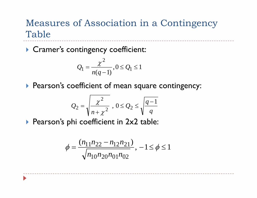
Measures of Association in a Contingency TableTable
Cramer’s contingency coefficient:2
Pearson’s coefficient of mean square contingency:
10,)1( 1
2
1 ≤≤−
= Qqn
Q χ
Pearson s coefficient of mean square contingency:
qqQ
nQ 10, 22
2
2−
≤≤+
=χ
χ
Pearson’s phi coefficient in 2x2 table:qn + χ
11,)(
02012010
21122211 ≤≤−−
= φφnnnnnnnn
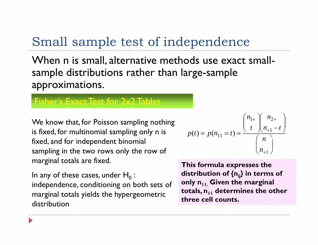
Small sample test of independenceSmall sample test of independenceWhen n is small, alternative methods use exact small-sample distributions rather than large-sample p g papproximations.Fisher’s Exact Test for 2x2 Tables
We know that, for Poisson sampling nothing is fixed, for multinomial sampling only n is
⎞⎛
⎟⎟⎠
⎞⎜⎜⎝
⎛−⎟⎟
⎠
⎞⎜⎜⎝
⎛
=== +
++
1
21
11 )()(n
tnn
tn
tnptpfixed, and for independent binomial sampling in the two rows only the row of marginal totals are fixed.
⎟⎟⎠
⎞⎜⎜⎝
⎛
+1nn
This formula expresses the In any of these cases, under H0 : independence, conditioning on both sets of marginal totals yields the hypergeometric
distribution of {nij} in terms of only n11. Given the marginal totals, n11 determines the other three cell countsdistribution three cell counts.

Small sample test of independenceSmall sample test of independenceFor 2x2 tables, independence is equivalent to the odds ratio θ = 1 To test H : θ = 1 the P-value is the odds ratio θ = 1. To test H0 : θ = 1, the P-value is the sum of certain hypergeometric probabilities. To illustrate, consider Ha: θ > 1. For the given marginal a g gtotals, tables having larger n11 have larger odds ratios and hence stronger evidence in favor of Ha.
Thus, the P-value equals P(n11 ≥ t0), where t0 denotes the observed value of n11.
This test for 2x2 tables is called Fisher’s exact test
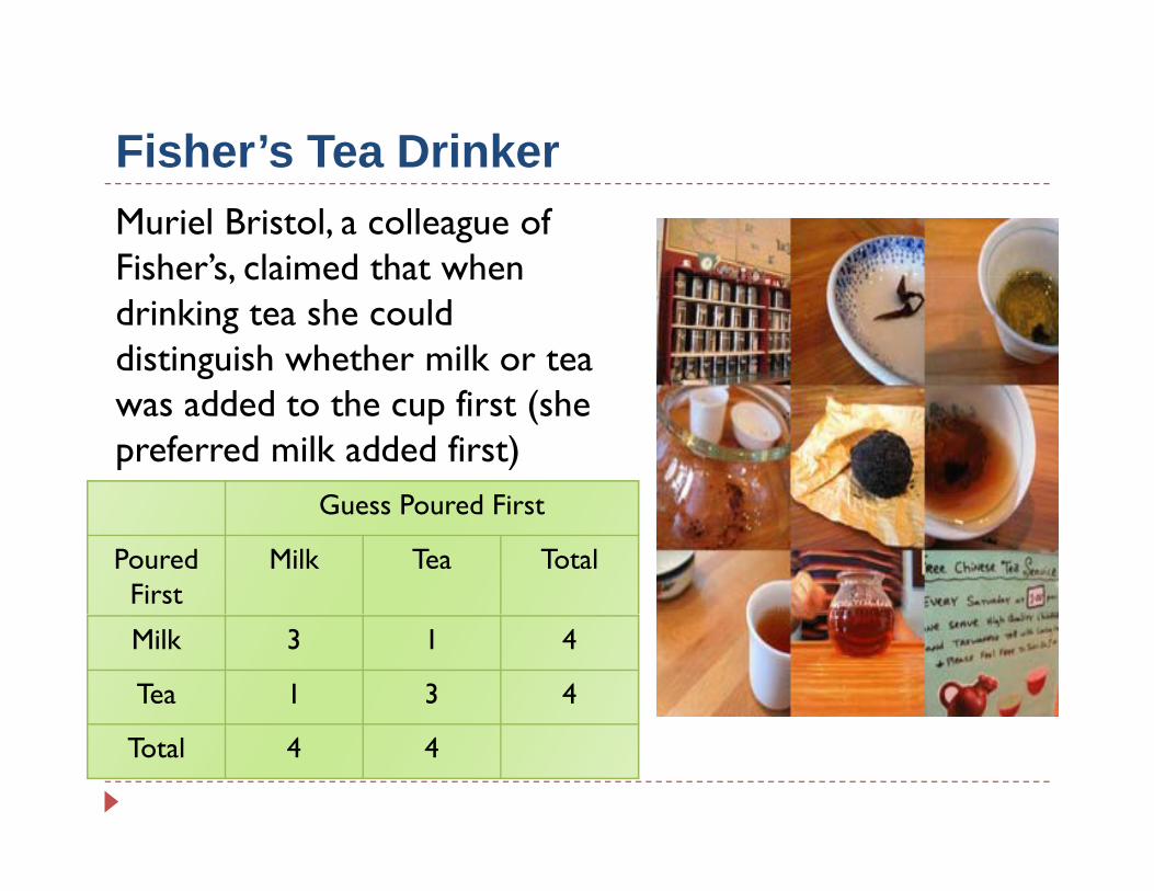
Fisher’s Tea DrinkerFisher s Tea DrinkerMuriel Bristol, a colleague of Fisher’s, claimed that when Fisher s, claimed that when drinking tea she could distinguish whether milk or tea was added to the cup first (she preferred milk added first)
Guess Poured FirstGuess Poured First
Poured First
Milk Tea Total
Milk 3 1 4
Tea 1 3 4
Total 4 4
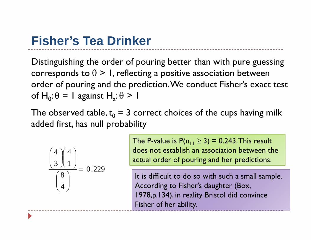
Fisher’s Tea DrinkerFisher s Tea DrinkerDistinguishing the order of pouring better than with pure guessing corresponds to θ > 1 reflecting a positive association between corresponds to θ > 1, reflecting a positive association between order of pouring and the prediction. We conduct Fisher’s exact test of H0: θ = 1 against Ha: θ > 1
The observed table, t0 = 3 correct choices of the cups having milk added first, has null probability
14
34
⎟⎟⎠
⎞⎜⎜⎝
⎛⎟⎟⎠
⎞⎜⎜⎝
⎛The P-value is P(n11 ≥ 3) = 0.243. This result does not establish an association between the actual order of pouring and her predictions.
229.0
48
13=
⎟⎟⎠
⎞⎜⎜⎝
⎛⎠⎝⎠⎝
It is difficult to do so with such a small sample. According to Fisher’s daughter (Box, 1978 p 134) in reality Bristol did convince 1978,p.134), in reality Bristol did convince Fisher of her ability.