catdograt dog3 rat45 cow676 barbara holland phylogenetics workhop, 16-18 august 2006 cat dog rat cow...

Cat Dog Rat

Dog 3

Rat 4 5

Cow 6 7 6

Barbara Holland

Phylogenetics Workhop, 16-18 August 2006

Cat

Dog

Rat

Cow

11

2

2 4

Distance Based Methodsfor estimating phylogenetic trees

How do we get distance data? Observed vs. actual distances Correcting for hidden changes Not all distances are “tree-like” Tree building: clustering methods

UPGMANeighbor-joining

Tree building: optimality criteriaLeast Squares

Overview

What do edge lengths represent? In some trees edges represent time, in which case all

modern sequences should be the same distance from the root.

Sometimes edge lengths represent the product μ∙t of the rate of change μ and time t in which case different tips can be different distances from the root provided that the rate has changed across the tree.

Cat

Dog

Rat

Cow

11

2

2 4

Distance matrices There are many ways of building phylogenetic

trees, one family of methods uses a distance matrix as a starting point.

A distance matrix is a table that indicates pairwise dissimilarity, for instance...

Cat Dog Rat Cow

Cat 0 2 4 7

Dog 2 0 5 6

Rat 4 5 0 3

Cow 7 6 3 0

A B C D

B 400 - - -

C 300 300 - -

D 250 150 250 -

E 250 250 500 200

Properties of distances

d(x,x) = 0 d(x,y) = d(y,x) d(x,y) + d(y,z) >= d(x,z) (the triangle inequality)

The distances used in phylogenetics always have the first two properties but sometimes not the third.

I want to build a tree - will any old distances do? Not all distances will be suitable for

building trees. Tree-building methods do not discriminate,

they will return a tree regardless of whether you give them roadmap distances or distances based on a sequence alignment.

Some distances are perfectly “tree-like”.

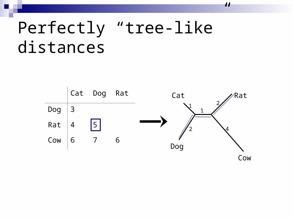
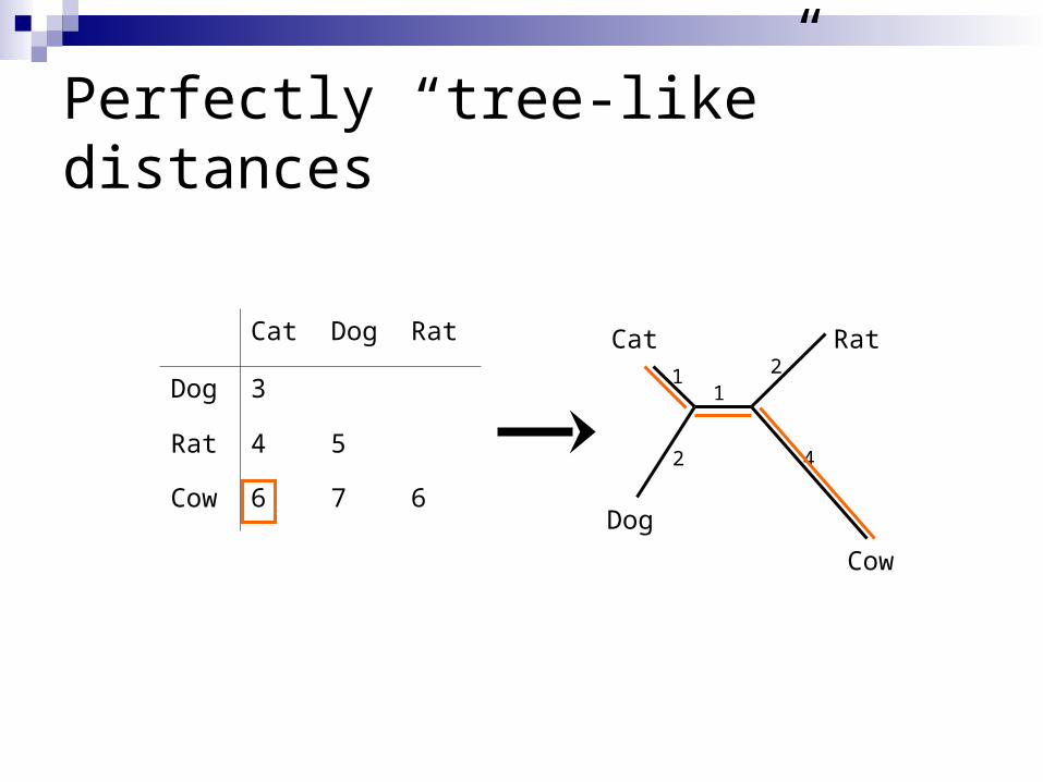
Perfectly “tree-like” distances

Cat Dog Rat

Dog 3

Rat 4 5

Cow 6 7 6

Cat

Dog

Rat

Cow

11

2

2 4

The 4-Point Condition Distances that fit exactly on a tree can be

characterised by a condition on any quartet i, j, k, l (i.e. it must hold true for any 4 taxa).

We write d(x,y) for the distance between x and y.Given 4 taxa i, j, k, l, of the 3 sums

d(i,j) + d(k,l) d(i,k) + d(j,l) d(i,l) + d(j,k)

The largest two are equal. Distances with this property are called additive,

because the weights on the paths along the tree add up to the values in the distance matrix.

Why is this true of tree-like distances?

i

j

k

l

i

j

k

l

i

j

k

l

d(i,j)+d(k,l) d(i,k)+d(j,l) d(i,l)+d(j,k)< =

Clock-like distances

An even stricter condition on distances is that they fit on a clock-like tree.

Distances with this property are called ultrametric.

time

i j k

d(i,k) = d(j,k) > d(i,j)

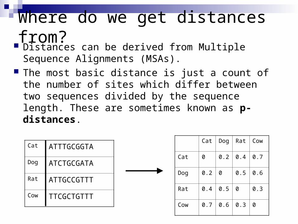
Distances can be derived from Multiple Sequence Alignments (MSAs).

The most basic distance is just a count of the number of sites which differ between two sequences divided by the sequence length. These are sometimes known as p-distances.

Cat ATTTGCGGTA

Dog ATCTGCGATA

Rat ATTGCCGTTT

Cow TTCGCTGTTT

Cat Dog Rat Cow

Cat 0 0.2 0.4 0.7

Dog 0.2 0 0.5 0.6

Rat 0.4 0.5 0 0.3

Cow 0.7 0.6 0.3 0

Where do we get distances from?

Other sources of distances

Immunological data Similarity between proteins A and B can be assessed by how well the

immune system responds to B after already having seen A.

DNA/DNA hybridization more similar DNA hybrids "melt" at higher temperatures

Fragment length polymorphism “Chop DNA up” using restriction enzymes. Amplify some fragments usign PCR Run the fragments out on an electrophoretic gel Compare profiles of different genomes

BLAST scores

Observed distances usually underestimate the true number of changes

ATTTGCGGTA ATCTGCGATA

ATTTGCGATA

Actual Changes = 2Observed Changes = 2

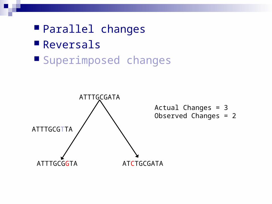
Parallel changes Reversals Superimposed changes


ATTCGCGATA




ATTTGCGATA


ATTCGCGATA



ATTTGCGATA


ATTTGCGTTA

Given a statistical model of how point mutations occur it is possible to estimate the true genetic distance from the observed distance.

Correcting for hidden changes

Correcting under a simple model The Jukes-Cantor model states that all

states {A,C,G,T} and all changes between states, e.g. A→C, are equally likely.

A G

C T

u/3

u/3

u/3

u/3 u/3u/3

As a mathematical conviencence imagine we have a rate 4u/3 of change to a random state, this includes the possibility of a state changing to itself.

A Poisson process The probability of no change at a site over time t is e-4/3ut

The probability of at least one event is then 1- e-4/3ut

The probability of at least one event that leads to a different state from the one we started at is ¾(1- e-4/3ut) as one time out of four we will “mutate” to the same base we started with.

The expected observed distance d given a true genetic distance of ut is d = ¾(1- e-4/3ut)

Inverting this formula gives our correction D = ut = -3/4 ln (1-4/3d)

Correction for hidden changes has been shown (both theoretically and by simulation studies) to improve accuracy.

However, this is not universally true. If data is clock-like then corrections will not

change the relative size of the distances However, the more complicated the model

is the larger the variance (error) of the distances will become.

Correcting for hidden changes

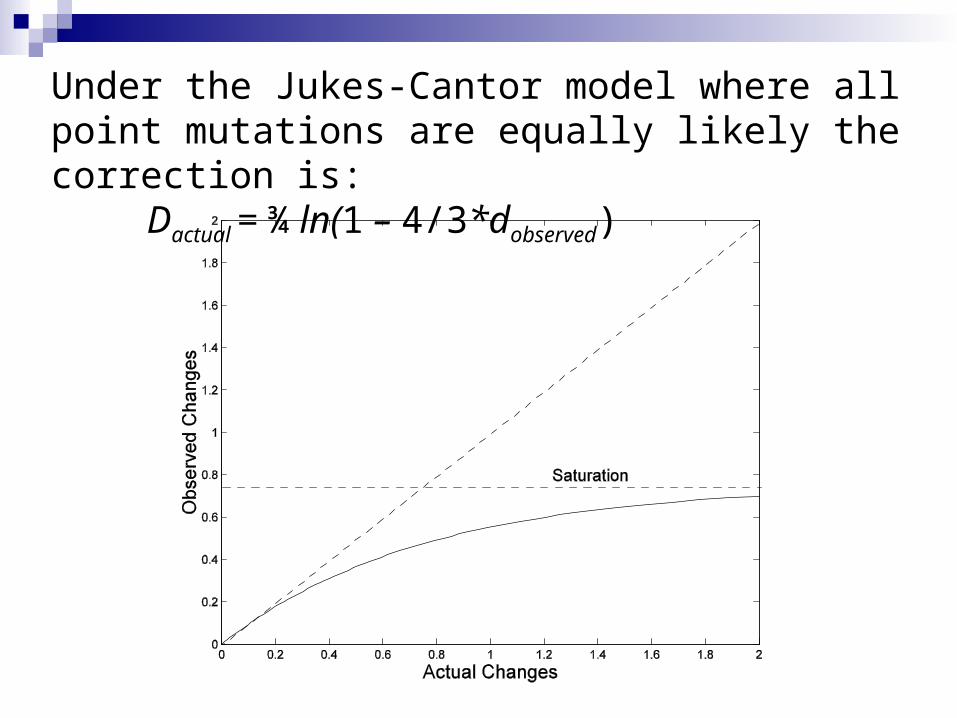
Under the Jukes-Cantor model where all point mutations are equally likely the correction is:

Dactual = ¾ ln(1 – 4/3*dobserved)

error

error

An interesting observation

Uncorrected distances always obey the triangle inequality d(x,y) + d(y,z) >= d(x,z)

But corrected distance do not. E.g. if sequences a and b differ at 10 / 100 sites

and sequences b and c differ at a different 10 / 100 sites the uncorrected distances are d(a,b) = d(b,c) = 0.1, d(a,c) = 0.2 and the corrected distances (under the JC model) are D(a,b) = D(b,c) = 0.107, D(a,c) = 0.233

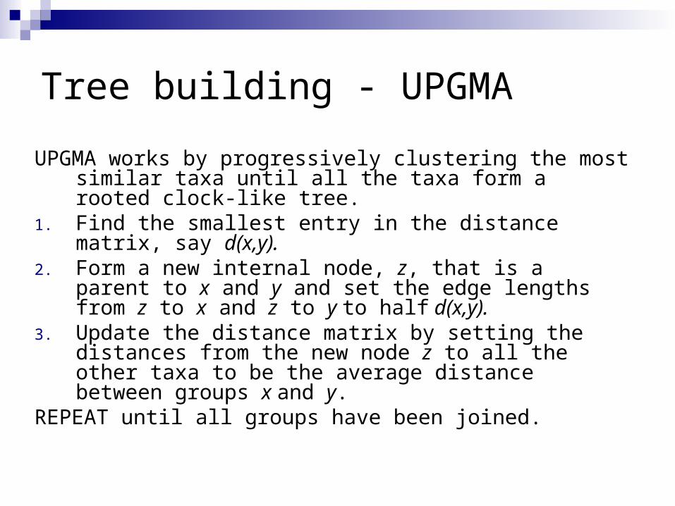
Tree building - UPGMA

UPGMA works by progressively clustering the most similar taxa until all the taxa form a rooted clock-like tree.

1. Find the smallest entry in the distance matrix, say d(x,y).

2. Form a new internal node, z, that is a parent to x and y and set the edge lengths from z to x and z to y to half d(x,y).

3. Update the distance matrix by setting the distances from the new node z to all the other taxa to be the average distance between groups x and y.

REPEAT until all groups have been joined.

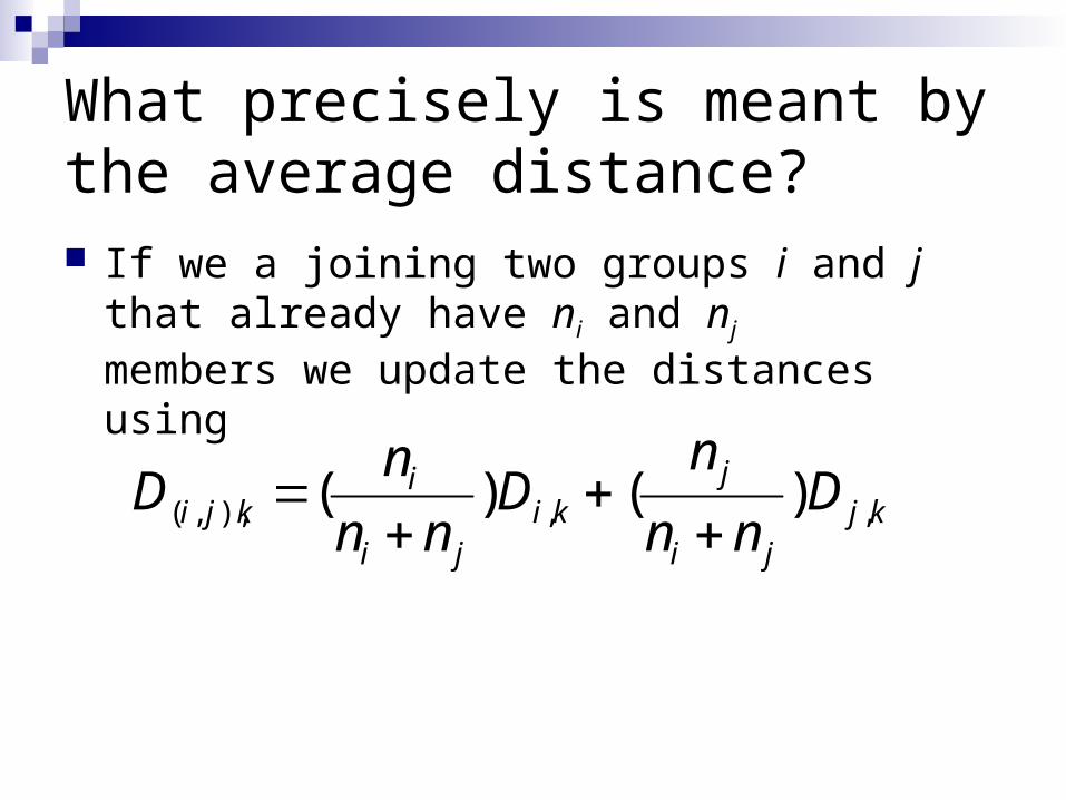
What precisely is meant by the average distance? If we a joining two groups i and j that already

have ni and nj members we update the distances using

kjji

jki

ji

ikji D

nn

nD

nn

nD ,,),,( )()(

d(i,j) A B C D E F A - B 2 - C 4 4 - D 4 4 2 - E 7 7 7 7 - F 5 5 5 5 6 - G 8 8 8 8 9 5

G

11

A B

I C

D

E

F

A

B

D

E

F

G

Step 2 - Cluster taxa A and B, form a new internal node ICalculate the lengths of the new edges d(A,I)=d(B,I)=1/2 d(A,B)=1

Step 1 – Find the smallest entry in the distance matrix

Step 3 – Update the distance matrixd(C,I) = ½(d(A,C) + d(B,C)) = 4 etc...

C

Step 2 - Cluster taxa C and D, form a new internal node IICalculate the lengths of the new edges d(C,II)=d(D,II)=1/2 d(C,D)=1

11

A B

I

E

F

11

C D

II

11

A B

I C

D

E

FG

d(i,j) I (A+B) C D E F

I (A+B) -

C 4 -

D 4 2 -

E 7 7 7 -

F 5 5 5 6 -

G 8 8 8 9 5

Step 1 – Find the smallest entry in the distance matrix

Step 3 – Update the distance matrixd(I,II)=1/2(d(I,C)+d(I,D)) = 4d(E,II) = ½(d(E,C) + d(E,D)) = 7 etc...

G

A B

I

A

B

C

DE

F

C D

EF

G

G

A B

I

E

FG

C D

II

A B C D

I IIIII

E

FG

I II

IIIIV

A B C D F

EG

I II

IIIIV

A B C D F E

G

V0.4

3.83.4

0.9

11

11

1 1

0.5

2.5I II

IIIIV

A B C D F E

V

G

VI

And so on...

...until we have a rooted tree.

But, is it the right tree?

d(i,j) A B C D E F A - B 2 - C 4 4 - D 4 4 2 - E 7 7 7 7 - F 5 5 5 5 6 - G 8 8 8 8 9 5

1

A

B

C D

E

G

F

11

11

1

1

1

14

4

0.4

3.8

3.4

0.9

11

11

11

0.5

2.5III

III

IV

A B C D F E

V

G

VI

=

The tree that matches the distances is not recovered by UPGMA.

UPGMA is not consistent for additive distances

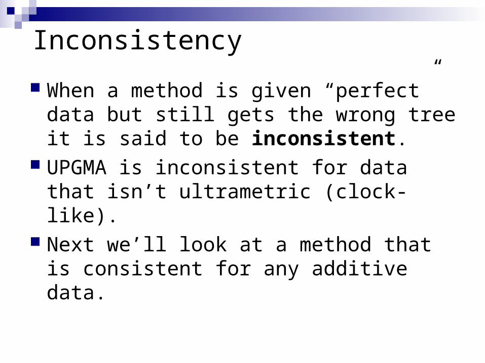
Inconsistency

When a method is given “perfect” data but still gets the wrong tree it is said to be inconsistent.

UPGMA is inconsistent for data that isn’t ultrametric (clock-like).

Next we’ll look at a method that is consistent for any additive data.

Neighbor-joining (NJ)

NJ works by progressively clustering taxa until all the taxa form an unrooted tree.

1. Rather than using the distance matrix directly to determine which taxa should be clustered at each stage, NJ uses the S matrix where

S(i,j) = (N-2)d(i,j) - R(i) - R(j)

N is the number of taxa.

R(i) is the sum of the ith row in the distance matrix.

R(j) is the sum of the jth row in the distance matrix.

2. Find the smallest entry in the S matrix, say S(x,y).

3. Form a new internal node, z, that is a parent to x and y and calculate the edge lengths from z to x and z to y.

d(x,z) = 1/(2(N-2))[(N-2)d(x,y) + R(x) – R(y)]d(y,z) = d(x,y) – d(x,z)

4. Update the distance matrixd(w,z) = ½ (d(x,w) + d(y,w) – d(x,y))

REPEAT until only two things are left to be joined.

NJ Example

Cat Dog Rat

Dog 3

Rat 4 5

Cow 6 7 6

Cat Dog Rat

Dog -22

Rat -20 -20

Cow -20 -20 -22

D= S=

R(cat) = 13R(dog) = 15R(rat) = 15R(cow) = 19

e.g. S(cat,dog) = (4-2)x3 – 13 – 15 = -22S(cat,rat) = (4-2)x4 – 13 – 15 = -20

Step 1

NJ Example

Cat Dog Rat

Dog 3

Rat 4 5

Cow 6 7 6

Cat Dog Rat

Dog -22

Rat -20 -20

Cow -20 -20 -22

D= S=

Cat

Dog

Rat

Cow

zStep 3d(cat,z) = ¼[2d(cat,dog) + R(cat) – R(dog)]

= ¼ [6 + 13 – 15]= 1

d(dog,z) = 3-1= 2

Step 1 Step 2

Cat

Dog

Rat

Cow

z

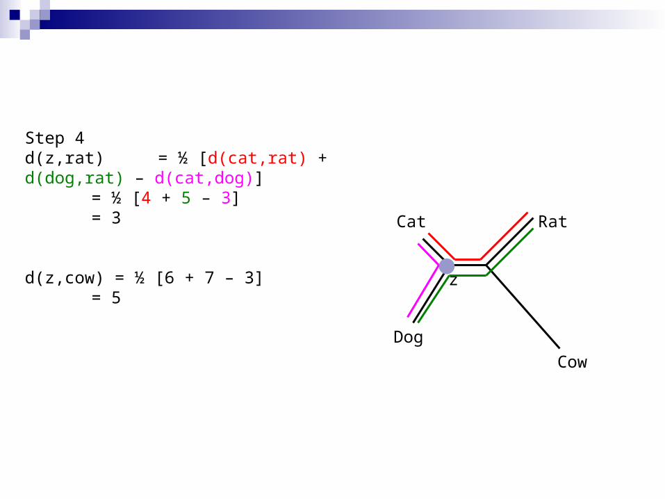
Step 4d(z,rat) = ½ [d(cat,rat) + d(dog,rat) – d(cat,dog)]

= ½ [4 + 5 – 3]= 3

d(z,cow) = ½ [6 + 7 – 3]= 5

Global vs Local methods UPGMA and NJ are local construction methods.

At each step they pick they best pair of taxa to cluster, once a decision is made it cannot be unmade. This makes these methods very fast.

There are also global methods for making trees based on distances. These evaluate an optimality criterion on each possible tree and then pick the tree with the best score. Examples of global methods for distance data include least squares and minimum evolution. Because the number of trees grows very quickly with the number of taxa, these methods are slow.

Least Squares

We would like the path lengths on the tree we choose to be as close as possible to the corresponding values in the distance matrix.

With additive data we can always find a tree where the path length distances and the distance matrix match exactly. However, most data isn’t perfect...

We can try and minimise the discrepency between the observed distances and the tree distances using a least squares approach.

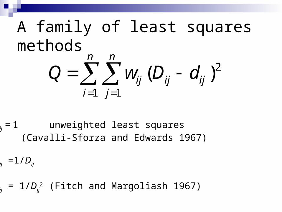
A family of least squares methods

n

i

n

jijijij dDwQ

1 1

2)(

wij = 1 unweighted least squares (Cavalli-Sforza and Edwards 1967)

wij =1/Dij

wij = 1/Dij2 (Fitch and Margoliash 1967)

Picking the best weights for a given tree

The tree distances dij can be represented by the equation

k

kkijij exd ,

where xij,k is an indicator variable that is 1 if edge k lies on the path from i to j and 0 otherwise.

We want to find edge weights ek that minimise

n

i

n

j kkkijijij exDwQ

1 1

2, )(

The indicator variables can be expressed in matrix format

E

AB

C

D

e1

e2

e3

e4

e5

e6 e7

1 1 1 0 0 0 01 1 0 1 1 0 01 1 0 1 0 0 11 0 0 0 0 1 00 0 1 1 1 0 00 0 1 1 0 0 10 1 1 0 0 1 00 0 0 0 1 0 10 1 0 1 1 1 00 0 0 0 0 1 1

X =

Each row of X corresponds to a path in the tree

We can write D = Xe

DAB

DAC

DAD

DAE

DBC

DBD

DBE

DCD

DCE

DDE

D =

e1

e2

e3

e4

e5

e6

e7

e =

Experience the joy of linear algebra

D=Xe

XTD = (XTX)e

e = (XTX)-1XTD

This assumes that the weights wij = 1

Minimum evolution

Uses the least squares method to fit the branch lengths for each tree

BUT uses a different optimality criterion than least squares.

Prefers the tree with the shortest sum of branch lengths

Review Observed distances derived from sequence alignments

will always underestimate the true number of mutations. Hence it is ususally a good idea to correct for these hidden changes.

Clustering methods like UPGMA and Neighbor-joining are very fast as they only make local decisions and never backtrack. These methods are often used as a starting point for heuristic searches.

There are also optimality criteria that use distances as input, e.g. Least squares and minimum evolution.

Review Not all distances can be fit perfectly onto a tree. Methods can be inconsistent, for example for

some non-clocklike distances UPGMA is guaranteed to recover the wrong tree.

UPGMA is consistent for clock-like distances and NJ is consistant for any additive distances.

catdograt dog3 rat45 cow676 barbara holland phylogenetics workhop, 16-18 august 2006 cat dog rat cow...

Documents

different distances

actual distances

old distances

roadmap distances

j slide

tree building

properties of distances

true of tree