STATE HIGHWAY ADMINISTRATION

RESEARCH REPORT

CATALOG OF MATERIAL PROPERTIES FOR MECHANISTIC-EMPIRICAL PAVEMENT DESIGN

CHARLES W. SCHWARTZ RUI LI

UNIVERITY OF MARYLAND

Project number SP808B4F FINAL REPORT

January 2011

MD-11-SP808B4F

Martin O’Malley, Governor Anthony G. Brown, Lt. Governor

Beverley K. Swaim-Staley, Secretary Neil J. Pedersen, Administrator

The contents of this report reflect the views of the author who is responsible for the facts and the accuracy of the data presented herein. The contents do not necessarily reflect the official views or policies of the Maryland State Highway Administration. This report does not constitute a standard, specification, or regulation.

Technical Report Documentation Page1. Report No. MD-11-SP808B4F

2. Government Accession No. 3. Recipient's Catalog No.

4. Title and Subtitle Catalog of Material Properties for Mechanistic-Empirical Pavement Design

5. Report Date January 2011

6. Performing Organization Code

7. Author/s Charles W. Schwartz Rui Li

8. Performing Organization Report No.

9. Performing Organization Name and Address University of Maryland College Park MD 20742

10. Work Unit No. (TRAIS) 11. Contract or Grant No.

SP808B4F 12. Sponsoring Organization Name and Address Maryland State Highway Administration Office of Policy & Research 707 North Calvert Street Baltimore MD 21202

13. Type of Report and Period Covered

Final Report 14. Sponsoring Agency Code (7120) STMD - MDOT/SHA

15. Supplementary Notes 16. Abstract The new Mechanistic-Empirical Pavement Design Guide adopted by AASHTO represents a fundamental advance over the current 50-year old empirical pavement design procedures derived from the AASHTO Road Test. The goal is to provide more cost-effective and better-performing pavement designs for the traffic volumes, vehicle characteristics, pavement materials, construction/rehabilitation techniques, and performance demands of today and the future. The MEPDG design procedures are implemented in the new DARWin-ME software currently under development and scheduled for release in April 2011. Material characterization for the MEPDG, the focus of this report, is significantly more fundamental and extensive than in the previous empirically-based AASHTO pavement design methodology. A hierarchical input data scheme has been implemented in the MEPDG to permit varying levels of sophistication for specifying material properties, ranging from laboratory measured values (Level 1) to empirical correlations (Level 2) to default values (Level 3). The development of this type of organized database of material properties for the most common paving materials in Maryland was the primary objective of this study. The database that was developed was populated with information received from the Maryland State Highway Administration (SHA). It provides complete data management tools for adding future data as well as data display screens for MEPDG inputs that mirror the input screens in the MEPDG Version 1.100 software. These data display screens can be easily modified to mirror the DARWin-ME input screens once the DARWin-ME software has been finalized and released to the public. All of the detailed testing recommendations for each of the specific materials are compiled in the summary.

17. Key Words Paving material properties, material characterization, MEPDG

18. Distribution Statement: No restrictions This document is available from the Research Division upon request.

19. Security Classification (of this report) None

20. Security Classification (of this page) None

21. No. Of Pages 127

22. Price

Form DOT F 1700.7 (8-72) Reproduction of form and completed page is authorized.

Catalog of Material Properties for Mechanistic-Empirical Pavement Design

Final Report

SHA Project No. SP808B4F

UMD FRS No. 430011

Submitted to: Tim Smith, P.E.

Director, Office of Materials Technology Maryland State Highway Administration

Hanover, MD 21076

Report prepared by:

Charles W. Schwartz Professor

Rui Li

Graduate Research Assistant

Department of Civil and Environmental Engineering The University of Maryland College Park, MD 20742

January 2011

i

TABLE OF CONTENTS

 LIST OF TABLES ......................................................................................................................... iii LIST OF FIGURES ....................................................................................................................... vii EXECUTIVE SUMMARY ............................................................................................................. 1 1. INTRODUCTION ....................................................................................................................... 2 2. BINDER DATA .......................................................................................................................... 5 

2.1 MEPDG Input Requirements ................................................................................................ 5 2.2 Binder Data Received and Preliminary Analysis .................................................................. 5 2.3 Sensitivity Analysis of Level 1/2 vs. Level 3 Binder Property Data ................................... 24 2.4 Summary ............................................................................................................................. 25 

2.4.1 Testing Recommendations ........................................................................................... 25 2.4.3 Recommended MEPDG Inputs .................................................................................... 26 

3. HMA DATA .............................................................................................................................. 29 3.1 MEPDG Input Requirements .............................................................................................. 29 

3.1.1 New Construction/Reconstruction/Overlays ................................................................ 29 3.1.2 Rehabilitation ............................................................................................................... 31 

3.2 HMA Data Summary and Preliminary Analysis ................................................................. 32 3.3 Sensitivity Analyses for HMA Mixture Inputs .................................................................... 47 

3.3.1 Level 1 vs. Level 2 vs. Level 3 Dynamic Modulus ...................................................... 47 3.3.2 Thermal Properties ....................................................................................................... 50 

3.4 Summary ............................................................................................................................. 54 3.4.1 Testing Recommendations ........................................................................................... 54 3.4.2 Recommended MEPDG Inputs .................................................................................... 55 

4. PCC DATA ............................................................................................................................... 59 4.1 MEPDG Input Requirements .............................................................................................. 59 

4.1.1 New Construction/Reconstruction/Overlays ................................................................ 59 4.1.2 Rehabilitation ............................................................................................................... 62 

4.2 PCC Data Summary ............................................................................................................ 63 4.3 Sensitivity Analyses for PCC Inputs ................................................................................... 65 

4.3.1 Strength and Stiffness Properties .................................................................................. 65 4.3.2 Thermal Properties ....................................................................................................... 82 4.3.3 Shrinkage Properties ..................................................................................................... 83 

4.4 Summary ............................................................................................................................. 84 4.4.1 Testing Recommendations ........................................................................................... 84 

ii

4.4.2 Recommended MEPDG Inputs .................................................................................... 84 5. UNBOUND MATERIAL DATA ............................................................................................. 87 

5.1 MEPDG Input Requirements .............................................................................................. 87 5.2 Summary of Data and Preliminary Analysis ....................................................................... 90 5.3 Analyses of Unbound Material Properties ........................................................................... 96 

5.3.1 Stiffness Properties ....................................................................................................... 96 5.3.2 Hydraulic Properties ................................................................................................... 105 

5.4 Summary ........................................................................................................................... 114 5.4.1 Testing Recommendations ......................................................................................... 114 5.4.2 Recommended MEDPG Inputs .................................................................................. 115 

6. MATERIAL PROPERTIES DATABASE .............................................................................. 119 6.1 Introduction ....................................................................................................................... 119 6.2 Instructions for Using MatProp ......................................................................................... 119 

6.2.1 User Interface for Flexible Pavement Material Management ..................................... 121 6.2.2 User Interface for Rigid Pavement Material Management ......................................... 132 6.2.3 User Interface for Unbound Material ......................................................................... 133 

6.3 Database Structure ............................................................................................................. 135 7. SUMMARY OF RECOMMENDATIONS ............................................................................. 145 

7.1 Project Summary ............................................................................................................... 145 7.2 Testing Recommendations ................................................................................................ 145 

7.2.1 Asphalt Binders .......................................................................................................... 145 7.2.2 HMA Mixtures ........................................................................................................... 145 7.2.3 PCC Mixtures ............................................................................................................. 146 7.2.4 Unbound Materials ..................................................................................................... 147 

8. REFERENCES ........................................................................................................................ 148 

iii

LIST OF TABLES Table 1. Number of test records received from SHA. ..................................................................... 5 

Table 2. Legend for supplier code numbers in Figure 1 to Figure 3. .............................................. 6 

Table 3. Differences in predicted distresses using MEPDG Level 3 vs. Level 1 binder inputs. ... 25 

Table 4. Recommended Level 3 binder grade inputs for wearing courses/surface layers (OMT, 2006). ............................................................................................................................................. 27 

Table 5. MEPDG thermal conductivity and heat capacity inputs. (NCHRP, 2004). ..................... 30 

Table 6. Typical coefficient of thermal expansion ranges for common aggregates (NCHRP, 2004). ............................................................................................................................ 30 

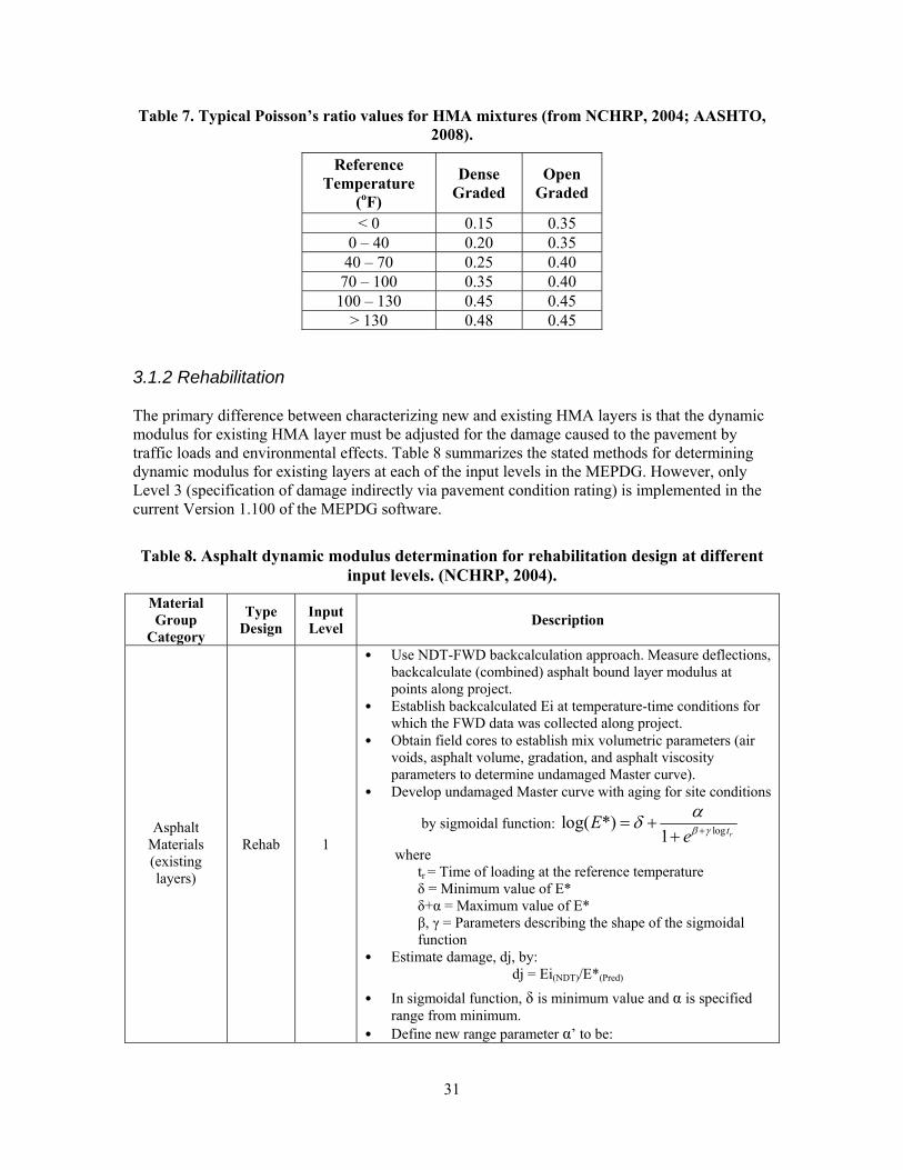
Table 7. Typical Poisson’s ratio values for HMA mixtures (from NCHRP, 2004; AASHTO, 2008). ............................................................................................................................................. 31 

Table 8. Asphalt dynamic modulus determination for rehabilitation design at different input levels. (NCHRP, 2004). ................................................................................................................. 31 

Table 9. Number of mixtures in database for each mixture size and type. Mixtures in bold italics were included in the correlation analyses. ..................................................................................... 33 

Table 10. Correlation analysis result for 9.5mm high polish mixes. ............................................. 45 

Table 11. Correlation analysis result for 12.5mm virgin mixes. ................................................... 45 

Table 12. Correlation analysis for 19.0mm virgin mixes. ............................................................. 46 

Table 13. Correlation analysis for 9.5mm RAP mixes. ................................................................. 46 

Table 14. Correlation analysis for 19.0mm RAP mixes. ............................................................... 47 

Table 15. Definitions of binder and traffic codes. ......................................................................... 47 

Table 16. Recommendation material property inputs for new HMA layers for Maryland conditions. ..................................................................................................................................... 55 

Table 17. Recommendation material property inputs for existing HMA layers for Maryland conditions. ..................................................................................................................................... 56 

Table 18. Recommendation thermal cracking inputs for new HMA layers for Maryland conditions. ..................................................................................................................................... 56 

Table 19. Level 3 inputs for Maryland HMA mixtures (based on material properties database at time of report). ............................................................................................................................... 57 

Table 20. SHA historical unit weights for Superpave mixes at 4% air voids (OMT, 2006). ........ 57 

Table 21. PCC elastic modulus estimation for new, reconstruction, and overlay design (NCHRP, 2004). ............................................................................................................................................. 60 

Table 22. PCC modulus of rupture estimation for new or reconstruction design and PCC overlay design (NCHRP, 2004). ................................................................................................................. 61 

Table 23. Estimation of PCC thermal conductivity, heat capacity, and surface absorptivity at various hierarchical input levels (NCHRP, 2004). ........................................................................ 62 

Table 24. Recommended condition factor values used to adjust moduli of intact slabs (from NCHRP, 2004). ................................................................................................................... 63 

iv

Table 25. Level 3 guidelines for in-place PCC elastic modulus (from NCHRP, 2004). ............... 63 

Table 26. Composition of Missouri DOT PCC mixes (ARA, 2009)............................................. 66 

Table 27. Mixture Properties from Missouri DOT. ....................................................................... 67 

Table 28. Predicted distresses using MEPDG Level 1, 2 and 3 PCC material property inputs based on “Gradation B” in Missouri DOT (ARA, 2009). ............................................................. 71 

Table 29. Predicted distresses using MEPDG Level 1, 2 and 3 PCC material property inputs based on “Gradation B Opt” in Missouri DOT (ARA, 2009). ...................................................... 72 

Table 30. Predicted distresses using MEPDG Level 1, 2 and 3 PCC material property inputs based on “Gradation D” in Missouri DOT (ARA, 2009). ............................................................. 73 

Table 31. Predicted distresses using MEPDG Level 1, 2 and 3 PCC material property inputs based on “Gradation D Opt” in Missouri DOT (ARA, 2009). ...................................................... 74 

Table 32. Predicted distresses using MEPDG Level 1, 2 and 3 PCC material property inputs based on “Gradation F” in Missouri DOT (ARA, 2009). .............................................................. 75 

Table 33. Baseline cases in OAT sensitivity analysis. Bold values are measured. ....................... 80 

Table 34. Generalized sensitivity indices of Ec and MOR at different ages to predictions. .......... 80 

Table 35. Recommended PCC thermal and shrinkage property inputs for Maryland conditions (all JPCP construction types). .............................................................................................................. 84 

Table 36. Recommended PCC mix property inputs for Maryland conditions. ............................. 85 

Table 37. Recommended strength and stiffness input properties for new PCC for Maryland conditions (new/reconstruction/rehabilitation designs). ................................................................ 85 

Table 38. Recommended strength and stiffness input properties for existing PCC for Maryland conditions (rehabilitation designs). ............................................................................................... 85 

Table 39. Ratio of laboratory MR to field backcalculated EFWD modulus values for unbound materials (AASHTO, 2008)........................................................................................................... 88 

Table 40. Models relating material index and strength properties to resilient modulus (NCHRP, 2004). ............................................................................................................................................. 89 

Table 41. MEPDG Level 3 default resilient moduli values at optimum moisture and density (AASHTO, 2008). ......................................................................................................................... 89 

Table 42. Number of test records received from SHA. ................................................................. 90 

Table 43. Recommended moduli for unbound materials from SHA Pavement Design Guide. .... 96 

Table 44. Suggested bulk stress θ (psi) values for use in design of granular base layers (AASHTO, 1993). ......................................................................................................................... 97 

Table 45. Stress states for various typical Maryland pavement structures. ................................... 97 

Table 46. Summary of stress state ranges from Richter (2002). ................................................. 100 

Table 47. Typical states of stress for Arizona flexible pavement sections (Andrei, 2003). ........ 100 

Table 48. Consolidated estimates of pavement stress states for Maryland conditions. ............... 101 

Table 49. SHA resilient modulus data evaluated at representative stress states. ......................... 102 

Table 50. MEPDG values of a, b, and ks for Eq. (6). .................................................................. 103 

v

Table 51. Recommendation material property inputs for unbound materials for Maryland conditions. ................................................................................................................................... 116 

Table 52. Typical Poisson’s ratio values for unbound granular and subgrade materials (NCHRP, 2004). ........................................................................................................................................... 116 

Table 53. Typical coefficient of lateral pressure for unbound granular, subgrade, and bedrock materials (NCHRP, 2004). .......................................................................................................... 117 

Table 54. Average properties for Maryland unbound materials (based on material property database at time of report). .......................................................................................................... 117 

vii

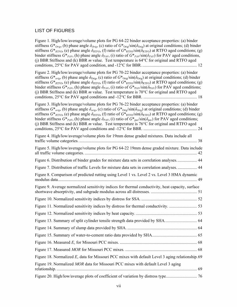
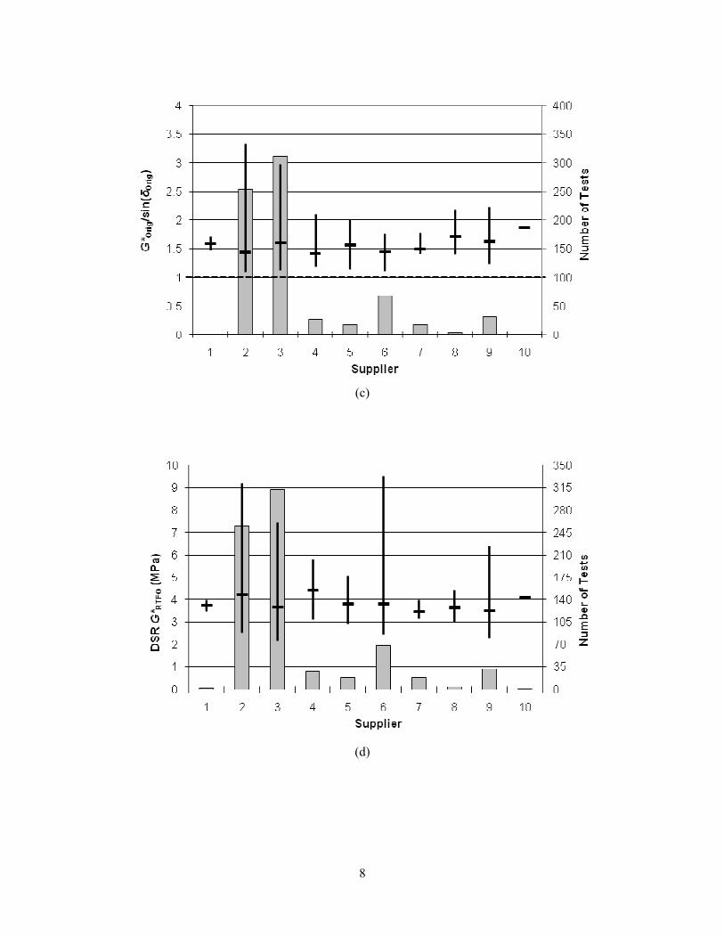
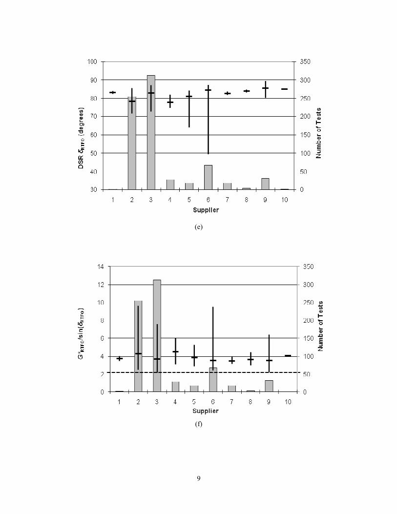
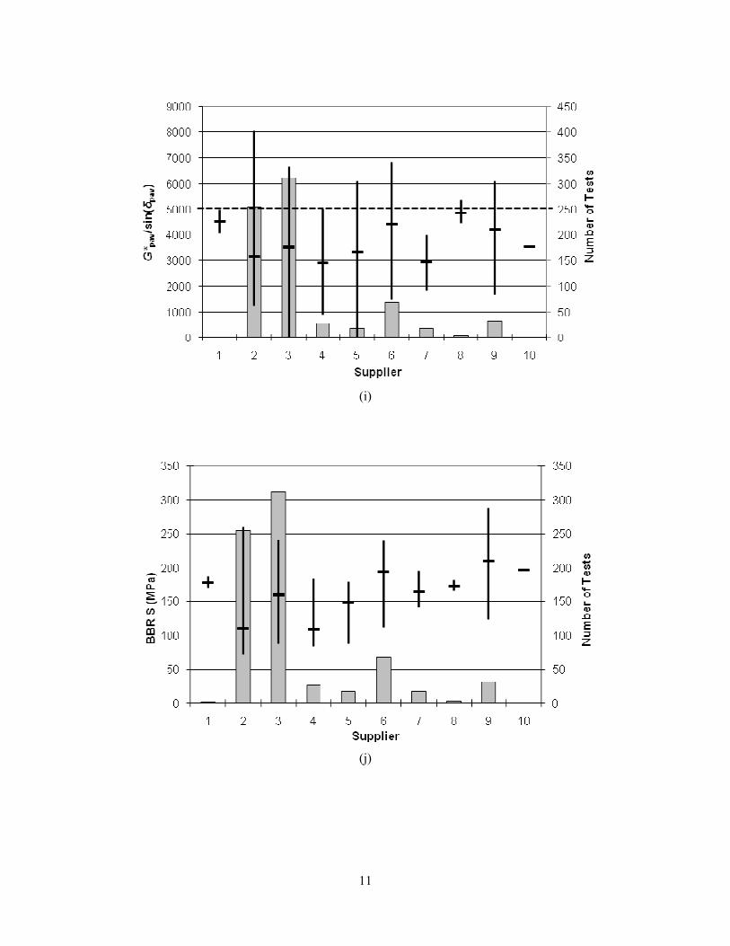
LIST OF FIGURES Figure 1. High/low/average/volume plots for PG 64-22 binder acceptance properties: (a) binder stiffness G*Orig, (b) phase angle δOrig, (c) ratio of G*Orig/sin(δOrig) at original conditions; (d) binder stiffness G*RTFO, (e) phase angle δRTFO, (f) ratio of G*RTFO/sin(δRTFO) at RTFO aged conditions; (g) binder stiffness G*PAV, (h) phase angle δPAV, (i) ratio of G*PAV/sin(δPAV) for PAV aged conditions, (j) BBR Stiffness and (k) BBR m value. Test temperature is 64°C for original and RTFO aged conditions, 25°C for PAV aged condition, and -12°C for BBR. ................................................... 12 

Figure 2. High/low/average/volume plots for PG 70-22 binder acceptance properties: (a) binder stiffness G*orig, (b) phase angle δOrig, (c) ratio of G*Orig/sin(δOrig) at original conditions; (d) binder stiffness G*RTFO, (e) phase angle δRTFO, (f) ratio of G*RTFO/sin(δRTFO) at RTFO aged conditions; (g) binder stiffness G*PAV, (h) phase angle δPAV, (i) ratio of G*PAV/sin(δPAV) for PAV aged conditions; (j) BBR Stiffness and (k) BBR m value. Test temperature is 70°C for original and RTFO aged conditions, 25°C for PAV aged conditions and -12°C for BBR. .................................................. 18 

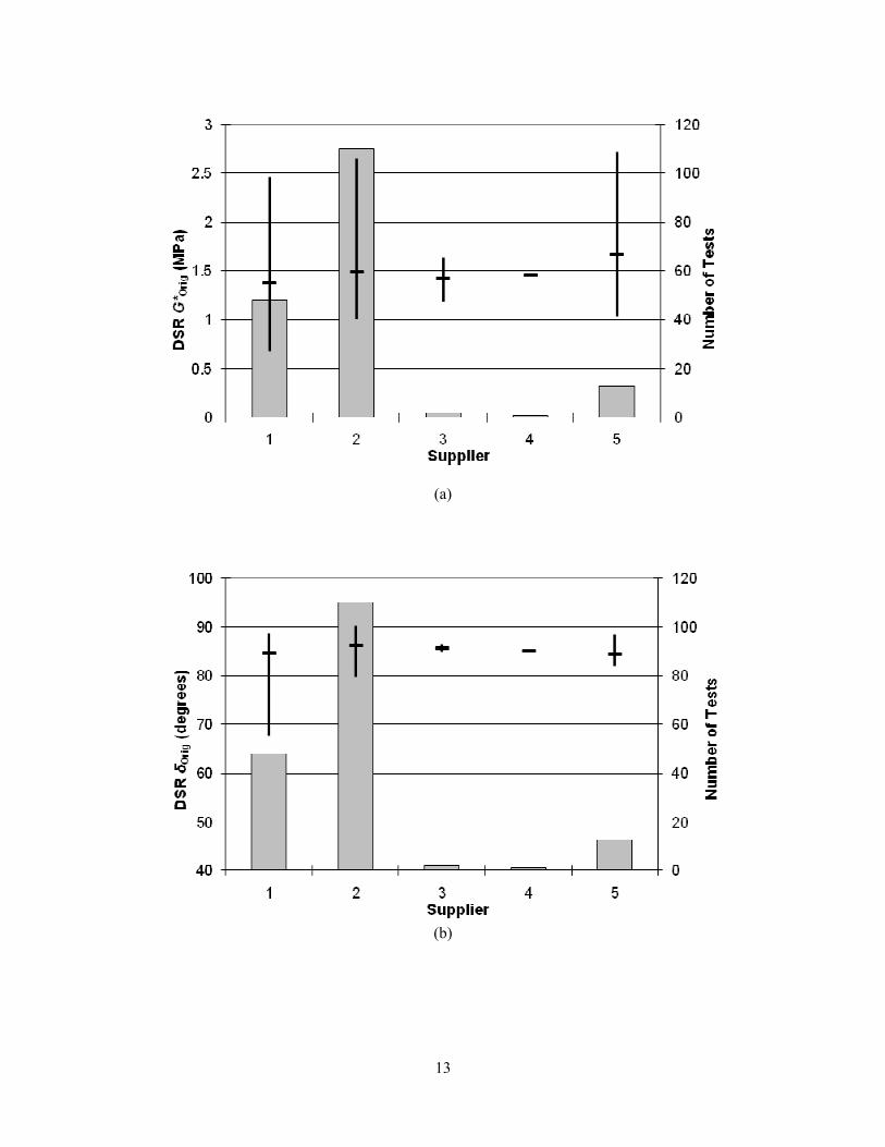
Figure 3. High/low/average/volume plots for PG 76-22 binder acceptance properties: (a) binder stiffness G*orig, (b) phase angle δorig, (c) ratio of G*Orig/sin(δOrig) at original conditions; (d) binder stiffness G*RTFO, (e) phase angle δRTFO, (f) ratio of G*RTFO/sin(δRTFO) at RTFO aged conditions; (g) binder stiffness G*PAV, (h) phase angle δPAV, (i) ratio of G*pav/sin(δpav) for PAV aged conditions; (j) BBR Stiffness and (k) BBR m value. Test temperature is 76°C for original and RTFO aged conditions, 25°C for PAV aged conditions and -12°C for BBR. .................................................. 24 

Figure 4. High/low/average/volume plots for 19mm dense graded mixtures. Data include all traffic volume categories. .............................................................................................................. 38 

Figure 5. High/low/average/volume plots for PG 64-22 19mm dense graded mixture. Data include all traffic volume categories. ......................................................................................................... 42 

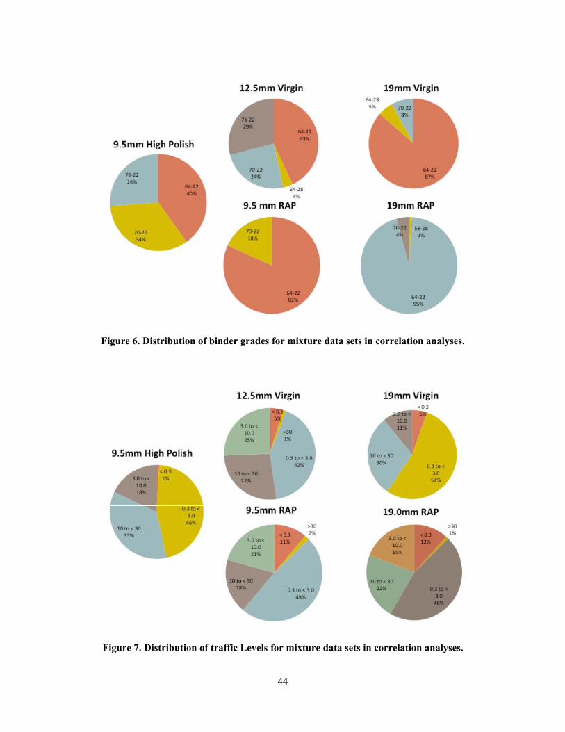
Figure 6. Distribution of binder grades for mixture data sets in correlation analyses. .................. 44 

Figure 7. Distribution of traffic Levels for mixture data sets in correlation analyses. .................. 44 

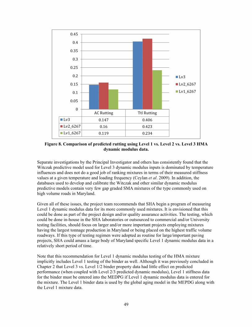
Figure 8. Comparison of predicted rutting using Level 1 vs. Level 2 vs. Level 3 HMA dynamic modulus data. ................................................................................................................................. 49 

Figure 9. Average normalized sensitivity indices for thermal conductivity, heat capacity, surface shortwave absorptivity, and subgrade modulus across all distresses. ........................................... 51 

Figure 10. Normalized sensitivity indices by distress for SSA. .................................................... 52 

Figure 11. Normalized sensitivity indices by distress for thermal conductivity. .......................... 53 

Figure 12. Normalized sensitivity indices by heat capacity. ......................................................... 53 

Figure 13. Summary of split cylinder tensile strength data provided by SHA. ............................. 64 

Figure 14. Summary of slump data provided by SHA. ................................................................. 64 

Figure 15. Summary of water-to-cement ratio data provided by SHA. ......................................... 65 

Figure 16. Measured Ec for Missouri PCC mixes. ........................................................................ 68 

Figure 17. Measured MOR for Missouri PCC mixes. ................................................................... 68 

Figure 18. Normalized Ec data for Missouri PCC mixes with default Level 3 aging relationship. 69 

Figure 19. Normalized MOR data for Missouri PCC mixes with default Level 3 aging relationship. ................................................................................................................................... 69 

Figure 20. High/low/average plots of coefficient of variation by distress type. ............................ 76 

viii

Figure 21. Predicted slab cracking value for different input levels and slab thicknesses for Gradation B mixture. ..................................................................................................................... 77 

Figure 22. Predicted slab cracking value for different input levels and slab thicknesses for Gradation B Opt mixture. .............................................................................................................. 77 

Figure 23. Predicted slab cracking value for different input levels and slab thicknesses for Gradation D mixture. ..................................................................................................................... 78 

Figure 24. Predicted slab cracking value for different input levels and slab thicknesses for Gradation D Opt mixture. .............................................................................................................. 78 

Figure 25. Predicted slab cracking compared to Level 1. ............................................................. 79 

Figure 26. Normalized sensitivity of predicted distresses to Ec and MOR values at different ages. ....................................................................................................................................................... 81 

Figure 27. Generalized Sensitivity Index of CTE of different Levels in MEPDG ........................ 83 

Figure 28. Averages and ranges of resilient modulus values at 95% compaction and optimum moisture content (includes all stress states). .................................................................................. 91 

Figure 29. Averages and ranges of optimum water contents......................................................... 92 

Figure 30. Averages and ranges of saturation levels at optimum moisture. .................................. 92 

Figure 31. Averages and ranges of maximum dry unit weights. ................................................... 93 

Figure 32. Averages and ranges of k2 and k3 for A-2-4 and A-7-5 soils. ...................................... 94 

Figure 33. Predicted vs. measured resilient moduli for A-2-4 and A-7-5 soils. ............................ 95 

Figure 34. Calculated stress states for granular base and subbase layers (Richter, 2002). ............ 98 

Figure 35. Calculated stress states for coarse grained subgrade soils (Richter, 2002). ................. 99 

Figure 36. Calculated stress states for fine grained subgrade soils (Richter, 2002). ..................... 99 

Figure 37. Predicted service life vs. subgrade resilient modulus; base modulus = 30,600 psi (Schwartz, 2009). ........................................................................................................................ 104 

Figure 38. Predicted service life vs. granular base modulus; subgrade modulus = 5000 psi (Schwartz, 2009). ........................................................................................................................ 104 

Figure 39. Examples of SWCC curves from the MEPDG. .......................................................... 106 

Figure 40. Predicted distresses for reference conditions (4 in. HMA, A-4 subgrade, 7 ft GWT depth, medium traffic). ................................................................................................................ 107 

Figure 41. Sensitivity of distresses to subgrade type at each location. ........................................ 108 

Figure 42. Influence of subgrade type on selected predicted distresses at all four climate locations (4 in. HMA thickness, 7 ft. GWT depth, medium traffic). .......................................................... 109 

Figure 43. Average modulus of top 2 feet of subgrade vs. time (4 in. HMA thickness, 7 ft. GWT depth, medium traffic). ................................................................................................................ 110 

Figure 44. Sensitivity to MR for all distresses at all locations. .................................................... 112 

Figure 45. Average absolute sensitivity to subgrade MR. ............................................................ 113 

Figure 46. Average absolute sensitivity to environmental variables. .......................................... 113 

Figure 47. Organization of MatProp database. ........................................................................... 119 

ix

Figure 48. Security warning. ....................................................................................................... 120 

Figure 49. Security alert. ............................................................................................................. 120 

Figure 50. Main menu. ................................................................................................................ 120 

Figure 51. “Show MEDPG HMA Input” screen for level 1 Asphalt Mix properties. ................. 122 

Figure 52. “Show MEDPG HMA Input” screen for level 2/3 Asphalt Mix properties. .............. 123 

Figure 53. “Show MEDPG HMA Input” screen for level 1/2 Asphalt Binder properties. ......... 124 

Figure 54. “Show MEDPG HMA Input” screen for level 3 Asphalt Binder properties. ............. 125 

Figure 55. “Show MEDPG HMA Input” screen for Asphalt General properties (all input levels). ..................................................................................................................................................... 126 

Figure 56. “Manage Binder Data” – main screen. ....................................................................... 127 

Figure 57. Add new binder. ......................................................................................................... 127 

Figure 58. Look up binder supplier. ............................................................................................ 127 

Figure 59. Add new supplier. ...................................................................................................... 128 

Figure 60. Look up terminal. ....................................................................................................... 128 

Figure 61. Add new terminal. ...................................................................................................... 128 

Figure 62. Data integrity checking before deleting terminal. ...................................................... 129 

Figure 63. Saving without completion. ....................................................................................... 129 

Figure 64. ID integrity checking. ................................................................................................ 129 

Figure 65. “Edit Binder Property” screen. ................................................................................... 129 

Figure 66. Delete without selection. ............................................................................................ 130 

Figure 67. “Manage HMA Data” – main screen. ........................................................................ 130 

Figure 68. Add HMA mixture. .................................................................................................... 131 

Figure 69. Edit dynamic modulus data. ....................................................................................... 131 

Figure 70. Attempt to add creep data without providing temperature. ........................................ 131 

Figure 71. Add creep compliance data. ....................................................................................... 132 

Figure 72. “Manage PCC Data” – main screen. .......................................................................... 132 

Figure 73. New PCC mixture. ..................................................................................................... 133 

Figure 74. “Manage Unbound Data” – main screen. ................................................................... 133 

Figure 75. Add unbound material. ............................................................................................... 134 

Figure 76. Edit unbound material. ............................................................................................... 134 

Figure 77. New testing condition. ............................................................................................... 134 

Figure 78. Edit testing condition. ................................................................................................ 135 

Figure 79. Add MR data. .............................................................................................................. 135 

Figure 80. Edit MR data. .............................................................................................................. 135 

Figure 81. Tables and relations for binder material data. ............................................................ 136 

x

Figure 82. Tables and relations for HMA mixture data. ............................................................. 136 

Figure 83. Tables and relations for PCC mixture data. ............................................................... 137 

Figure 84. Tables and relations for unbound material data. ........................................................ 138 

1

EXECUTIVE SUMMARY The new Mechanistic-Empirical Pavement Design Guide (MEPDG) developed in NCHRP Project 1-37A , refined in NCHRP Project 1-40D, and subsequently adopted by AASHTO represents a fundamental advance over the current 50-year old empirical pavement design procedures derived from the AASHTO Road Test. The overall goal of the MEPDG is to provide more cost-effective and better-performing pavement designs for the traffic volumes, vehicle characteristics, pavement materials, construction/rehabilitation techniques, and performance demands of today and the future. The MEPDG design procedures are implemented in the new DARWin-ME software currently under development and scheduled for release by AASHTO in April 2011. Support of the DARWin-3.1 software based on the older empirical design procedure will be discontinued shortly thereafter. Material characterization for the MEPDG, the focus of this report, is significantly more fundamental and extensive than in the previous empirically-based AASHTO pavement design methodology. A hierarchical input data scheme has been implemented in the MEPDG to permit varying levels of sophistication for specifying material properties, ranging from laboratory measured values (Level 1) to empirical correlations (Level 2) to default values (Level 3). Databases or libraries of typical material property inputs must be developed for the following categories:

• Binder properties (e.g., binder dynamic modulus G* and phase angle δ or binder viscosities η)

• HMA mechanical properties (e.g., dynamic modulus E* master curves—either measured directly or predicted empirically)

• PCC mechanical properties (e.g., elastic modulus Ec, modulus of rupture MOR)

• Unbound mechanical properties (e.g., resilient modulus Mr or k1-k3 values)

• Thermohydraulic properties (e.g., saturated hydraulic conductivity ksat)

The development of this type of organized database of material properties for the most common paving materials used in Maryland is the primary objective of the study described in this report. Separate chapters for each of the major material types (asphalt binders, hot mix asphalt concrete, Portland cement concrete, and unbound/subgrade materials) provide the following essential information for understanding and using the MEPDG: MEPDG Input Requirements New Construction/Reconstruction/Overlays Rehabilitation (Existing Layers) Data Available from Maryland SHA Analyses of MEDPG Inputs Level 1 vs. Level 2 vs. Level 3 Sensitivity Analyses Summary Testing Recommendations Recommended MEPDG Inputs For convenience, all of the detailed testing recommendations for each of the specific materials are compiled in the concluding summary chapter.

2

A comprehensive material property database developed in Microsoft Access 2007 accompanies this report. This database is initially populated with all information received from SHA. It provides complete data management tools for adding future data as well as data display screens for MEPDG inputs that mirror the input screens in the MEPDG Version 1.100 software. These data display screens can be easily modified to mirror the DARWin-ME input screens once the DARWin-ME software has been finalized and released to the public.

3

1. INTRODUCTION The new pavement design methodology developed in NCHRP Project 1-37A , refined in NCHRP Project 1-40D, and subsequently adopted by AASHTO (AASHTO, 2008) is based on mechanistic-empirical principles that are expected to be used in parallel with and eventually replace the current empirical pavement design procedures derived from the AASHO Road Test conducted in the late 1950’s (HRB, 1962). The new mechanistic-empirical pavement design guide (MEPDG) requires greater quantities and quality of input data in four major categories: traffic; material characterization; environmental factors; and pavement performance (for local calibration/validation). Material characterization for the mechanistic-empirical approach, the focus of this report, is significantly more fundamental and extensive than in the current empirically-based AASHTO Design Guide (AASHTO, 1993). The implementation plan developed by the University of Maryland (UMD) for the Maryland State Highway Administration (SHA) recommended a range of research projects to be completed in preparation for the MEPDG (Schwartz, 2007). One of the higher priority efforts identified in the plan was to catalog and compile existing material properties. This project final report addresses this need. A hierarchical input data scheme has been implemented in the MEPDG to permit varying levels of sophistication for specifying material properties, ranging from laboratory measured values (Level 1) to empirical correlations (Level 2) to default values (Level 3). It is expected that most states, including Maryland, will begin implementation of the new design procedure using Level 3 default inputs or Level 2 correlations that are relevant to their local materials and conditions and will, over time, supplement these with typical Level 1 measured data for their most common materials. To accomplish this, databases or libraries of typical material property inputs must be developed for the following categories:

- Binder properties (e.g., binder dynamic modulus G* and phase angle δ or binder viscosities η)

- HMA mechanical properties (e.g., dynamic modulus E* master curves—either measured directly or predicted empirically)

- PCC mechanical properties (e.g., elastic modulus Ec, modulus of rupture MOR)

- Unbound mechanical properties (e.g., resilient modulus Mr or k1-k3 values)

- Thermohydraulic properties (e.g., saturated hydraulic conductivity ksat)

The objective of the study described in this report is to develop this type of organized database of material properties for the most common paving materials used in Maryland. Note that this project provides an essential prerequisite for an eventual full local calibration/validation of the MEPDG for Maryland conditions. The work plan for accomplishing the research objective was organized into seven tasks:

Task 1: Database Design Task 2: Binder Properties Task 3: HMA Mechanical and Physical Properties Task 4: PCC Mechanical and Physical Properties Task 5: Unbound Mechanical and Physical Properties Task 6: Thermohydraulic Properties Task 7: Workshop and Final Report

4

The organization of this report closely mirrors the work plan. The principal difference is that the findings on thermohydraulic properties from Task 6 have been merged with the coverage of the mechanical and physical properties for each material type. The organization of the chapters of this report is thus: 1: Introduction 2: Binder Data 3: HMA Data 4: PCC Data 5: Unbound Material Data 6: Material Properties Database 7: Summary of Recommendations 8: References Each of the specific material Chapters 2 through 5 generally follows the same consistent organization: MEPDG Input Requirements New Construction/Reconstruction/Overlays Rehabilitation (Existing Layers) Data Available from Maryland SHA Analyses of MEDPG Inputs Level 1 vs. Level 2 vs. Level 3 Sensitivity Analyses Summary Testing Recommendations Recommended MEPDG Inputs The final Chapter 7 compiles in one location all of the detailed testing recommendations from each of the specific material Chapters 2 through 5. A comprehensive material property database developed in Microsoft Access 2007 accompanies this report. This database is initially populated with all information receive from SHA. It provides complete data management tools for adding future data as well as data display screens for MEPDG inputs that mirror the input screens in the MEPDG Version 1.100 software. Documentation of this database is provided in Chapter 6. A workshop summarizing the findings of this study was held at the Office of Materials Technology headquarters on July 23, 2010. This workshop was attended by approximately 20 SHA staff. In addition to this report, results from this study have appeared/will appear in part in published articles by Schwartz (2009), Schwartz and Li (2010), and Schwartz et al. (2011). Complete citations for these articles can be found in the reference list at the end of this report.

5

2. BINDER DATA 2.1 MEPDG Input Requirements The binder properties required at each of the input levels in the MEPDG are as follows:

• Level 1: Shear stiffness G* and phase angle δ at multiple temperatures at a frequency of ω = 10 radians/sec (AASHTO T315)

• Level 2: Same as Level 1 • Level 3: Default A-VTS viscosity temperature susceptibility parameters based on

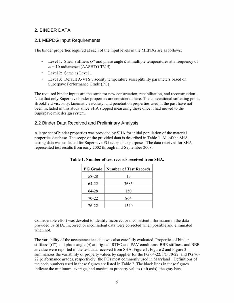
Superpave Performance Grade (PG) The required binder inputs are the same for new construction, rehabilitation, and reconstruction. Note that only Superpave binder properties are considered here. The conventional softening point, Brookfield viscosity, kinematic viscosity, and penetration properties used in the past have not been included in this study since SHA stopped measuring these once it had moved to the Superpave mix design system. 2.2 Binder Data Received and Preliminary Analysis A large set of binder properties was provided by SHA for initial population of the material properties database. The scope of the provided data is described in Table 1. All of the SHA testing data was collected for Superpave PG acceptance purposes. The data received for SHA represented test results from early 2002 through mid-September 2008.

Table 1. Number of test records received from SHA.

PG Grade Number of Test Records

58-28 15

64-22 3685

64-28 150

70-22 864

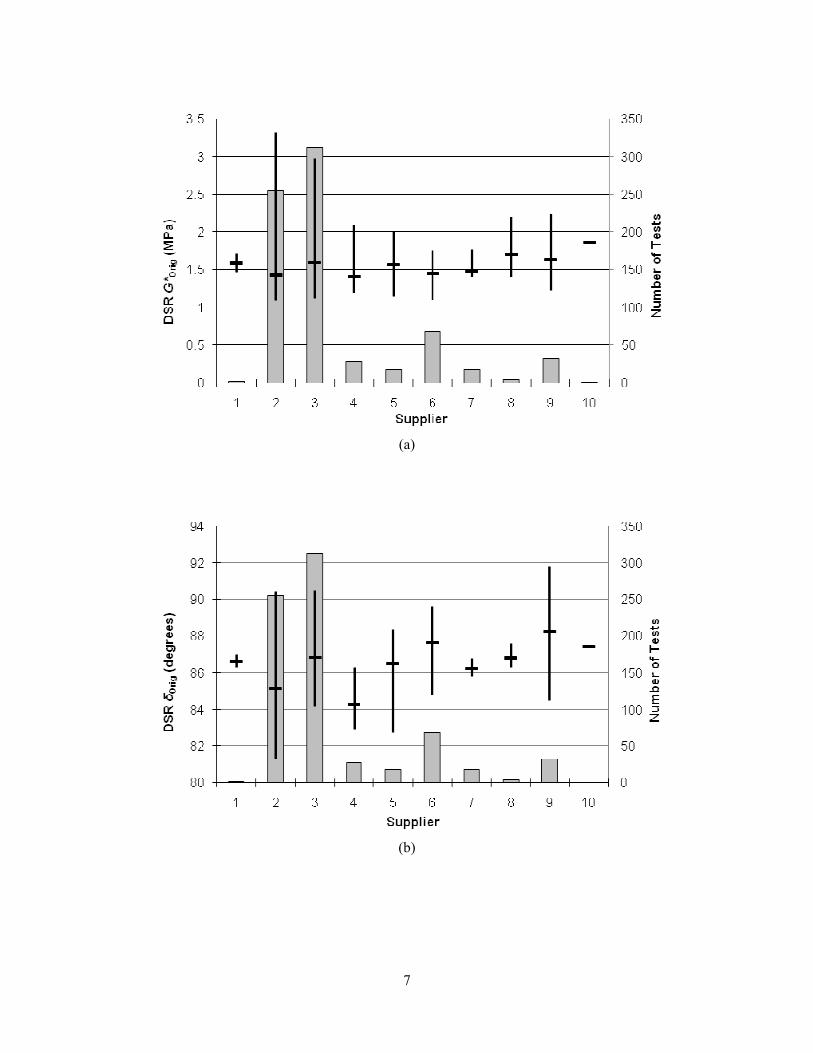
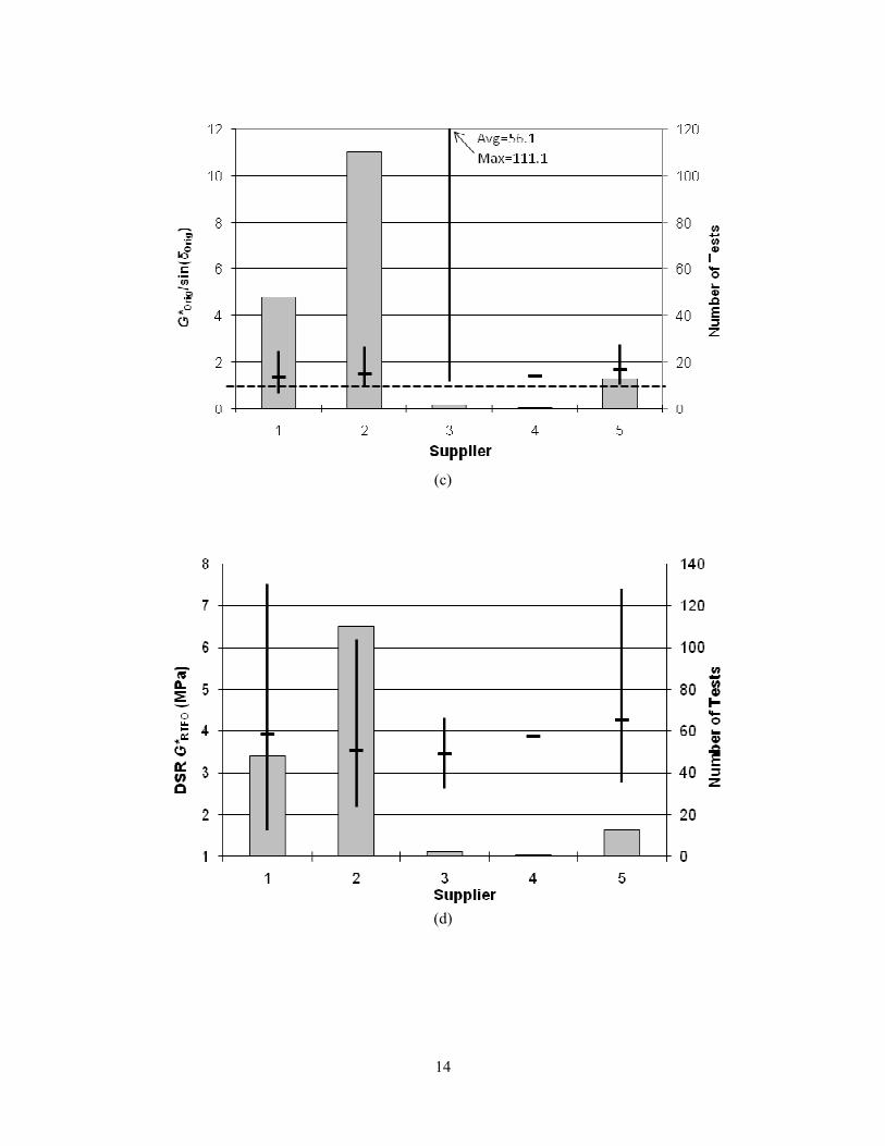
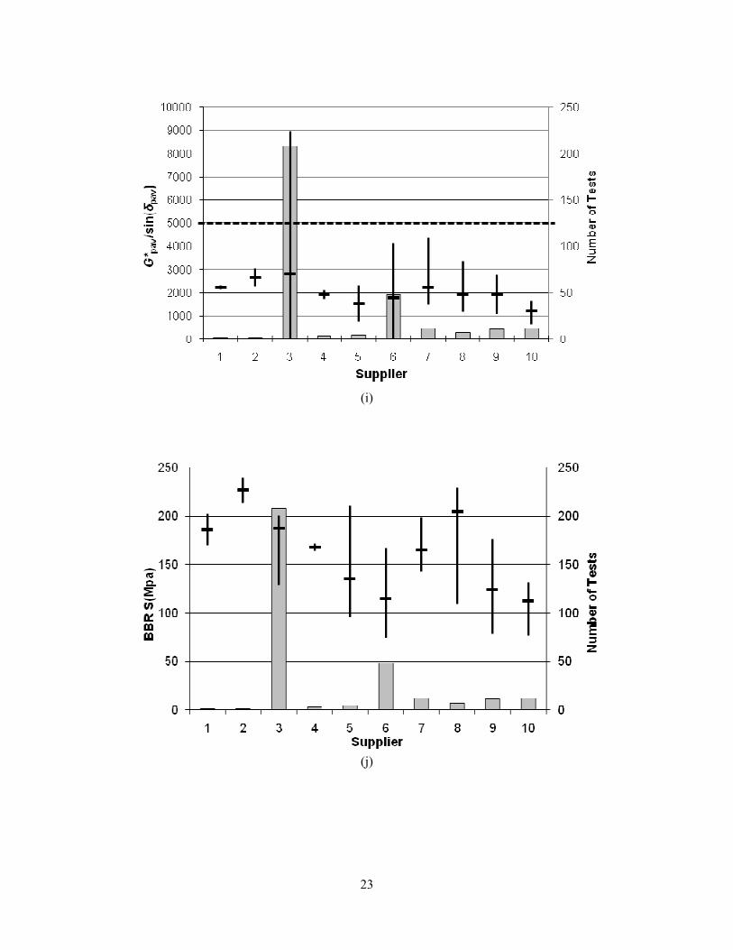
76-22 1540 Considerable effort was devoted to identify incorrect or inconsistent information in the data provided by SHA. Incorrect or inconsistent data were corrected when possible and eliminated when not. The variability of the acceptance test data was also carefully evaluated. Properties of binder stiffness (G*) and phase angle (δ) at original, RTFO and PAV conditions, BBR stiffness and BBR m value were reported in the test data received from SHA. Figure 1, Figure 2 and Figure 3 summarizes the variability of property values by supplier for the PG 64-22, PG 70-22, and PG 76-22 performance grades, respectively (the PGs most commonly used in Maryland). Definitions of the code numbers used in these figures are listed in Table 2. The black lines in these figures indicate the minimum, average, and maximum property values (left axis), the gray bars

6

summarize the number of test data in each category (right axis). Note that the thick dashed lines in Chart (c), Chart (f) and Chart (i) in each figure indicate the specification limits for G*/sinδ at each aging condition. There are no specification values for BBR stiffness or BBR m value. From these figures it can be seen that nearly all data fall within the specification limits for the original and RTFO conditions. Some data are significantly above the maximum limit for the PAV aged condition (i.e. Supplier 2 and 6 in Figure 2.1(i)). The reasons and consequences of these violations of the acceptance specification conditions are unknown. However, since the stiffness properties at PAV condition represent binder performance at low temperature, this should not have much practical significance in Maryland where low temperature cracking is not a problem. Furthermore, since binder data at the PAV condition is not an input in MEPDG, it will not affect the MEPDG predictions.

Table 2. Legend for supplier code numbers in Figure 1 to Figure 3.

Code Figure 1 Figure 2 Figure 3

1 Associated Asphalt Chevron Associated Asphalt

2 Chevron Citgo Chevron

3 Citgo Marathon Ashland Citgo

4 ESM ASPHALT, LLC NuStar Asphalt Refining, LLC Conoco Phillips

5 Koch Valero ESM ASPHALT, LLC

6 Marathon Ashland Koch

7 NuStar Asphalt Refining, LLC Marathon Ashland

9 United NuStar Asphalt Refining, LLC

10 Valero SEM Materials

7

(a)

(b)

8

(c)

(d)

9

(e)

(f)

10

(g)

(h)

11

(i)

(j)

12

(k)

Figure 1. High/low/average/volume plots for PG 64-22 binder acceptance properties: (a) binder stiffness G*Orig, (b) phase angle δOrig, (c) ratio of G*Orig/sin(δOrig) at original

conditions; (d) binder stiffness G*RTFO, (e) phase angle δRTFO, (f) ratio of G*RTFO/sin(δRTFO) at RTFO aged conditions; (g) binder stiffness G*PAV, (h) phase angle δPAV, (i) ratio of

G*PAV/sin(δPAV) for PAV aged conditions, (j) BBR Stiffness and (k) BBR m value. Test temperature is 64°C for original and RTFO aged conditions, 25°C for PAV aged condition,

and -12°C for BBR.

13

(a)

(b)

14

(c)

(d)

15

(e)

(f)

16

(g)

(h)

17

(i)

(j)

18

(k)

Figure 2. High/low/average/volume plots for PG 70-22 binder acceptance properties: (a) binder stiffness G*orig, (b) phase angle δOrig, (c) ratio of G*Orig/sin(δOrig) at original

conditions; (d) binder stiffness G*RTFO, (e) phase angle δRTFO, (f) ratio of G*RTFO/sin(δRTFO) at RTFO aged conditions; (g) binder stiffness G*PAV, (h) phase angle δPAV, (i) ratio of

G*PAV/sin(δPAV) for PAV aged conditions; (j) BBR Stiffness and (k) BBR m value. Test temperature is 70°C for original and RTFO aged conditions, 25°C for PAV aged conditions

and -12°C for BBR.

19

(a)

(b)

20

(c)

(d)

21

(e)

(f)

22

(g)

(h)

23

(i)

(j)

24

(k)

Figure 3. High/low/average/volume plots for PG 76-22 binder acceptance properties: (a) binder stiffness G*orig, (b) phase angle δorig, (c) ratio of G*Orig/sin(δOrig) at original conditions;

(d) binder stiffness G*RTFO, (e) phase angle δRTFO, (f) ratio of G*RTFO/sin(δRTFO) at RTFO aged conditions; (g) binder stiffness G*PAV, (h) phase angle δPAV, (i) ratio of G*pav/sin(δpav)

for PAV aged conditions; (j) BBR Stiffness and (k) BBR m value. Test temperature is 76°C for original and RTFO aged conditions, 25°C for PAV aged conditions and -12°C for BBR.

As documented later in Chapter 6, binder property tables for the MatProp database have been designed to accommodate both the current Superpave acceptance testing data provided by SHA and to permit future entry of full Superpave characterization data—i.e., DSR at multiple temperatures at RTFO conditions, BBR, etc. No conventional binder viscosity data (e.g., Brookfield viscosity, penetration, etc.) were provided by SHA. Therefore, no provisions for storing these older superseded viscosity characteristics have been included in the database design. 2.3 Sensitivity Analysis of Level 1/2 vs. Level 3 Binder Property Data Since acceptance testing is performed at a single temperature, it does not provide sufficient information for Level 1 or Level 2 Superpave binder characterization in the MEPDG. Therefore, only Level 3 inputs—PG grade—can be provided for the binders based on the data received from SHA. The major question regarding appropriate input levels for binder property data is: “Are there significant differences in predicted performance from the MEPDG using Level 1, 2, or 3 binder property data?” A review of the literature found no published studies that specifically addressed this question. Therefore, the project team conducted a very limited comparison analysis using the MEPDG for typical Maryland conditions. The analysis scenario was a simple pavement section

25

consisting of 6 inches of HMA (19mm dense graded, PG 76-22) over 15 inches of granular base (A-1-b) over subgrade (A5, upper 12 inches compacted). The HMA was based on the control mixture at the FHWA ALF test, which was designed using aggregates and unmodified binders similar to those commonly used in dense graded mixtures in Maryland. Level 2 binder test data was extracted from the FHWA ALF research reports. Level 3 defaults were assumed for all other material properties. Traffic was set at 950 trucks per day in the design lane (TTC4 for Principal Arterials – Interstates and Defense Highways) and Baltimore (BWI) weather history (interpolated with DC and IAD weather history) was taken as the climate input. Reliability was set at the MEPDG default 90% level for all distresses. The distresses predicted by the MEPDG using Level 3 vs. Level 1 inputs for this scenario are summarized in Table 3 (recall that Level 2 binder inputs are the same as Level 1). The MEPDG consistently predicts slightly higher distress magnitudes using Level 1 than Level 3 inputs for this scenario, but the differences are very small. Although this comparison is extremely limited (i.e., just one binder, albeit of a type commonly used in Maryland), a reasonable conclusion is that, based just on the binder influence alone, it does not seem worthwhile for SHA to embark on a large-scale Level 1/Level 2 binder testing program. However, as will be shown in Chapter 3, this conclusion is superseded when considering Level 1 vs. Level 3 HMA properties. Level 1 stiffness data for the binder must be entered into the MEPDG if Level 1 dynamic modulus data is entered for the mixture. The Level 1 binder data is used by the global aging model in the MEPDG along with the Level 1 mixture data. Table 3. Differences in predicted distresses using MEPDG Level 3 vs. Level 1 binder inputs.

Distress Type Distress Magnitude Level 3 Inputs Level 1 Inputs Δ (%) Level 3 1

Longitudinal Cracking (ft/mile) 470 501 +6.2 Alligator Cracking(% wheelpath) 2.31 2.43 +4.9 Transverse Cracking (ft/mile) 0 0 -- Subgrade Rutting (in) 0.2655 0.2663 +0.3 Base Rutting(in) 0.0998 0.1015 +1.7 HMA Rutting(in) 0.250 0.265 +5.7 Total Rutting (in) 0.615 0.633 +2.8 IRI (in/mile) 120.2 121.0 +0.7

2.4 Summary

2.4.1 Testing Recommendations The sensitivity of predicted pavement performance to Level 1 vs. Level 2 vs. Level 3 binder inputs appears slight. Therefore, based only on this criterion there would be little purpose for SHA collection of Level 1 or 2 binder data. As will be shown in Chapter 3, however, predicted pavement performance can be substantially different using MEPDG Level 1 vs. Level 2 vs. Level 3 HMA mixture inputs. There is consequently a motivation for SHA collection of Level 1 HMA dynamic modulus values. However, input of Level 1 HMA properties also requires input of Level 1/2 binder data. It is recommended that SHA develop a policy of full binder characterization on major projects and that the test results be entered into the material property database so that typical Level 1/2

26

properties can be input into the MEPDG in the future. The testing frequency for full binder characterization should match the recommendations for HMA dynamic modulus testing as detailed in Chapter 3.

2.4.3 Recommended MEPDG Inputs Only binder acceptance data has been collected by SHA to date. This is insufficient for Level 1 or Level 2 inputs in the MEPDG. Consequently, only Level 3 binder data can be input at this time. Until Level 1 binder data become available, it is recommended that the PG grade for Level 3 input be selected according to the binder recommendations in the SHA/OMT Pavement Design Guide:

1. All HMA layers other than wearing course/surface layer: PG 64-22

2. HMA wearing courses/surface layers other than gap-graded: See Table 4.

3. Gap-graded HMA wearing courses/surface layers: PG 76-22

27

Table 4. Recommended Level 3 binder grade inputs for wearing courses/surface layers (OMT, 2006).

(a) Wearing surface for all counties except Garrett

(b) Wearing surface for Garrett county

29

3. HMA DATA 3.1 MEPDG Input Requirements

3.1.1 New Construction/Reconstruction/Overlays Dynamic modulus is the principal mechanical property input for HMA in the MEPDG. The methods for specifying dynamic modulus at each of the input levels in the MEDPG are as follows:

• Level 1: Laboratory-measured dynamic modulus |E*| at multiple temperatures and loading frequencies (AASHTO TP62). In addition, Level 1/2 binder stiffness and phase angle data are required for the global aging model.

• Level 2: Gradation and volumetric data for use in the Witczak |E*| predictive model: percent retained above the 3/4” sieve; percent retained above the 3/8” sieve; percent retained above the #4 sieve; percent passing the #200 sieve; effective volumetric binder content (%); and in-place air voids (%). In addition, Level 1/2 stiffness and phase angle data are also required for the binder.

• Level 3: Gradation and volumetric data for use in the Witczak |E*| predictive model. Default binder stiffness properties are based on the Superpave Performance Grade for the binder.

Creep compliance and low temperature tensile strength are additional mechanical properties required in the MEPDG for predicting thermal cracking distress. The methods for specifying these properties at each of the input levels in the MEPDG are as follows:

• Level 1: Laboratory-measured creep compliance at three temperatures and various loading times and laboratory-measured tensile strength at 14oF (AASHTO T322).

• Levels 2 and 3: Default creep compliance and low temperature tensile strength determined from empirical relations built into the MEPDG; empirical relations are functions of mix volumetric and binder viscosity properties.

HMA thermal properties required by the MEPDG include:

• Thermal conductivity and heat capacity: see Table 5.

• Surface shortwave absorptivity (SSA), which quantifies the fraction of available solar energy that is absorbed by a given surface. Lighter and more reflective surfaces have lower SSA values. The recommended methods for determining SSA at each of the input levels are: o Level 1: Estimate through laboratory testing. However there is no AASHTO certified

testing standards for this. o Levels 2 and 3: Default values based on surface characteristics:

- Weathered asphalt (gray) 0.80-0.90 - Fresh asphalt(black) 0.90-0.98

30

• Aggregate coefficient of thermal expansion (also sometimes called coefficient of thermal contraction): see Table 6.

Additional physical mixture properties required for all input levels are Poisson’s ratio and total unit weight. Both of these properties have relatively small influence on predicted pavement performance. There is no national test protocol for measuring Poisson’s ratio for HMA; the default Level 3 values recommended in the MEDPG are given in Table 7. HMA total unit weight can be measured in the laboratory according to AASHTO T166 or estimated based on previous construction records.

Table 5. MEPDG thermal conductivity and heat capacity inputs. (NCHRP, 2004).

Table 6. Typical coefficient of thermal expansion ranges for common aggregates (NCHRP, 2004).

31

Table 7. Typical Poisson’s ratio values for HMA mixtures (from NCHRP, 2004; AASHTO, 2008).

Reference Temperature

(oF)

Dense Graded

Open Graded

< 0 0.15 0.35 0 – 40 0.20 0.35

40 – 70 0.25 0.40 70 – 100 0.35 0.40 100 – 130 0.45 0.45

> 130 0.48 0.45

3.1.2 Rehabilitation The primary difference between characterizing new and existing HMA layers is that the dynamic modulus for existing HMA layer must be adjusted for the damage caused to the pavement by traffic loads and environmental effects. Table 8 summarizes the stated methods for determining dynamic modulus for existing layers at each of the input levels in the MEPDG. However, only Level 3 (specification of damage indirectly via pavement condition rating) is implemented in the current Version 1.100 of the MEPDG software.

Table 8. Asphalt dynamic modulus determination for rehabilitation design at different input levels. (NCHRP, 2004).

Material Group

Category

Type Design

Input Level Description

Asphalt

Materials (existing layers)

Rehab 1

• Use NDT-FWD backcalculation approach. Measure deflections, backcalculate (combined) asphalt bound layer modulus at points along project.

• Establish backcalculated Ei at temperature-time conditions for which the FWD data was collected along project.

• Obtain field cores to establish mix volumetric parameters (air voids, asphalt volume, gradation, and asphalt viscosity parameters to determine undamaged Master curve).

• Develop undamaged Master curve with aging for site conditions

by sigmoidal function: loglog( *)1 rt

Eeβ γ

αδ += ++

where tr = Time of loading at the reference temperature δ = Minimum value of E* δ+α = Maximum value of E* β, γ = Parameters describing the shape of the sigmoidal function

• Estimate damage, dj, by: dj = Ei(NDT)/E*(Pred)

• In sigmoidal function, δ is minimum value and α is specified range from minimum.

• Define new range parameter α’ to be:

32

α’ = (1-dj) α • Develop field damaged master curve using α’ rather than α

2

• Use field cores to establish mix volumetric parameters (air voids, asphalt volume, gradation, and asphalt viscosity parameters to define Ai-VTSi values).

• Develop by predictive equation, undamaged master curve with aging for site conditions from mix input properties determined from analysis of field cores.

• Conduct indirect Mr laboratory tests, using revised protocol developed at University of Maryland for NCHRP 1-28A from field cores.

• Use 2 to 3 temperatures below 70°F • Estimate damage, dj, at similar temperature and time rate of

load conditions: dj = Mri/E*(Pred)

• In sigmoidal function , δ is minimum value and α is specified range from minimum. Define new range parameter α’ to be:

• α’ = (1-dj) α • Develop field damaged master curve using α’ rather than α

3

• Use typical estimates of mix modulus prediction equation (mix volumetric, gradation and binder type) to develop undamaged master curve with aging for site layer.

• Using results of distress/condition survey, obtain estimate for pavement rating (excellent, good, fair, poor, very poor)

• Use a typical tabular correlation relating pavement rating to pavement layer damage value, dj.

• In sigmoidal function, δ is minimum value and α is specified range from minimum. Define new range parameter α’ to be:

α’ = (1-dj) α • Develop field damaged master curve using α’ rather than α

Other existing HMA layer properties are specified in the MEPDG as follows:

• Creep compliance and low temperature tensile strength: Not required for existing HMA layers.

• Thermal conductivity and heat capacity: Same as for new construction (Table 5). • Surface shortwave absorptivity: Not required for existing HMA layers. • Aggregate coefficient of expansion: Not required for existing HMA layers. • Unit weight and Poisson’s ratio: Same as for new construction (Table 7).

3.2 HMA Data Summary and Preliminary Analysis A large set of asphalt mixture design properties was provided by SHA for initial population of the material properties database. The scope of the provided data is described in Table 9. The date range for these data is unknown, other than that they were received from SHA in Fall 2008. As for the binder data in Chapter 2, the project team devoted considerable effort identifying incorrect or inconsistent information in the data. Incorrect or inconsistent data were corrected when possible and eliminated when not.

33

Table 9. Number of mixtures in database for each mixture size and type. Mixtures in bold italics were included in the correlation analyses.

HMAS Mix Type Number

4.75mm High Polish 1 Virgin 25

9.5mm Gap Graded 10 High Polish 122 RAP 126 Shingle 5 Virgin 68

12.5mm Gap Graded 40 High Polish 56 RAP 84 Shingle 6 Virgin 86

19.0mm Gap Graded 1 High Polish 24 RAP 122 Shingle 8 Virgin 37

25.00mm RAP 50 Virgin 20

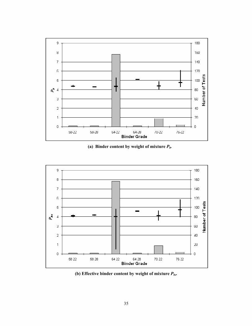
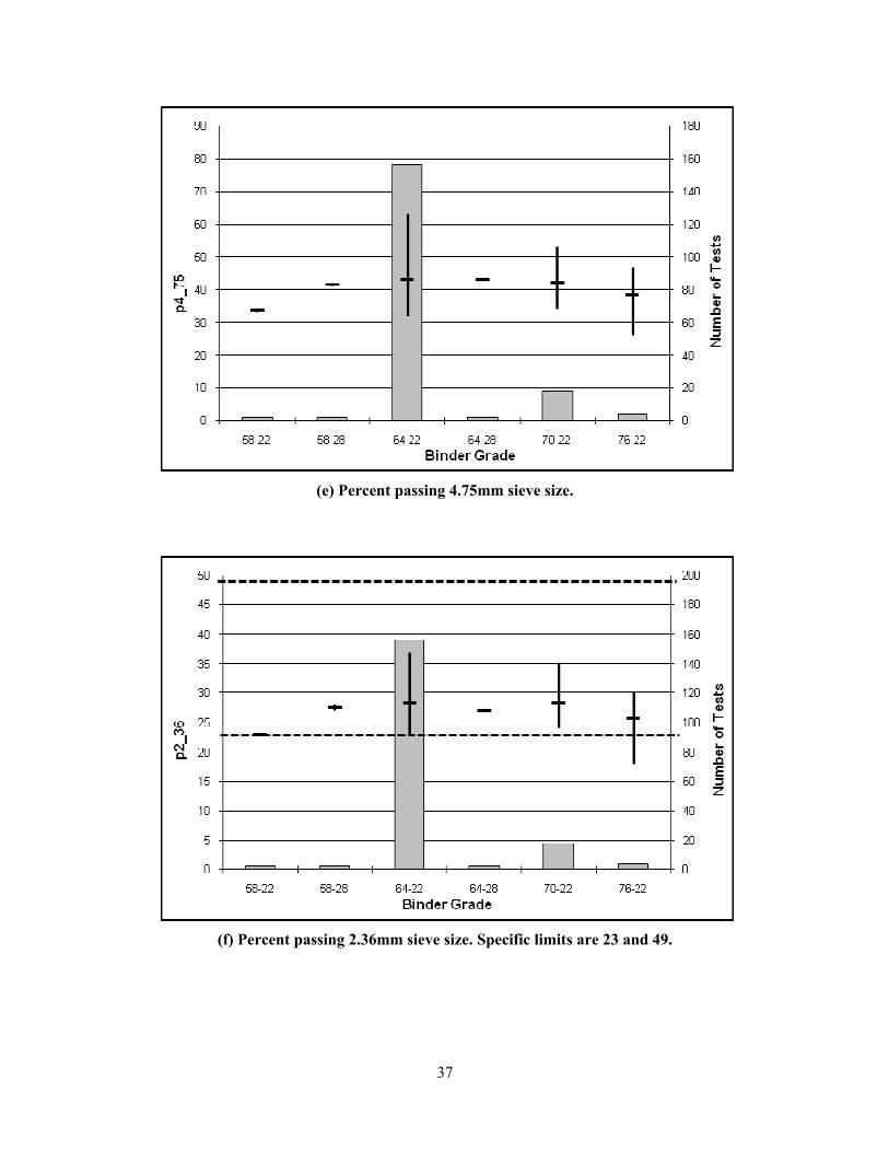
37.5mm RAP 6 The HMA mixture information provided by SHA is limited to volumetric and gradation data suitable for Level 3 input to the MEPDG. No measured dynamic modulus, creep compliance, low temperature tensile strength, or thermal property values suitable for Level 1 inputs were provided. Although the volumetric and gradation data provided by SHA are sufficient for Level 2 inputs, the required corresponding Level 2 binder data are absent. The simplest way to categorize typical Level 3 volumetric and gradation MEPDG inputs for Maryland materials is to define them as a function only of mix type (e.g., gap- vs. dense-graded) and mix size (e.g., 19 mm nominal maximum aggregate size). To explore whether this is possible, trends in volumetric and gradation data for a given mix type and mix size as a function of binder grade and/or traffic level were examined, as illustrated in Figure 4 and Figure 5 respectively for 19 mm dense-graded mixtures. In these figures, the grey bars indicate the number of tests included in the database for each subset of data (right axis), the heavy black vertical lines indicate the ranges of the data (left axis), and the heavy black short horizontal lines indicate the mean values (left axis). Noteworthy observations regarding the data in these figures include the following:

• The PG 64-22 is the most common binder in the data set (Figure 4). This is not surprising, as this is the recommended binder for Maryland environmental conditions under all but the heaviest traffic conditions.

• The ranges of the volumetric properties are largest for the PG 64-22 mixtures (Figure 4). This is most likely because these are the most common mixtures, and thus the opportunity for encountering especially high or low values is large.

34

• The ranges of the volumetric properties for the PG 70-22 and PG 76-22 mixtures (Figure

4), although not as large as for the PG 64-22 data, are still surprisingly large, especially given that the number of mixtures using these binders is comparatively small. Air voids Va is the only exception to this trend (Figure 4h). Note that the PG 70-22 and PG 76-22 binders are generally specified by SHA for its premium mixtures—e.g., SMA surface mixtures on heavily trafficked interstate highways.

• The 0.3-3M ESAL traffic category is the most common design condition (Figure 5). Very few mix designs fall into the >30M ESAL very high traffic condition.

• Overall, the range of the volumetric properties is moderate to large for the four lowest traffic categories (Figure 5). There are insufficient mixtures in the highest traffic category to portray the property ranges accurately.

There were no consistent overall trends in the mean values for the volumetric and gradation properties either with regard to binder grade or traffic level. This is consistent with expectations, as the SHA mix design specifications for these properties are not functions of binder grade or traffic level.

35

(a) Binder content by weight of mixture Pb.

(b) Effective binder content by weight of mixture Pbe.

36

(c) Voids in mineral aggregates VMA. Minimum VMA is 13.

(d) Dust to effective binder ratio D/Pbe.

37

(e) Percent passing 4.75mm sieve size.

(f) Percent passing 2.36mm sieve size. Specific limits are 23 and 49.

38

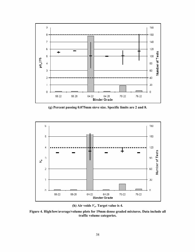
(g) Percent passing 0.075mm sieve size. Specific limits are 2 and 8.

(h) Air voids Va. Target value is 4.

Figure 4. High/low/average/volume plots for 19mm dense graded mixtures. Data include all traffic volume categories.

39

(a) Binder content by weight of mixture Pb.

(b) Effective binder content by weight of mixture Pbe.

40

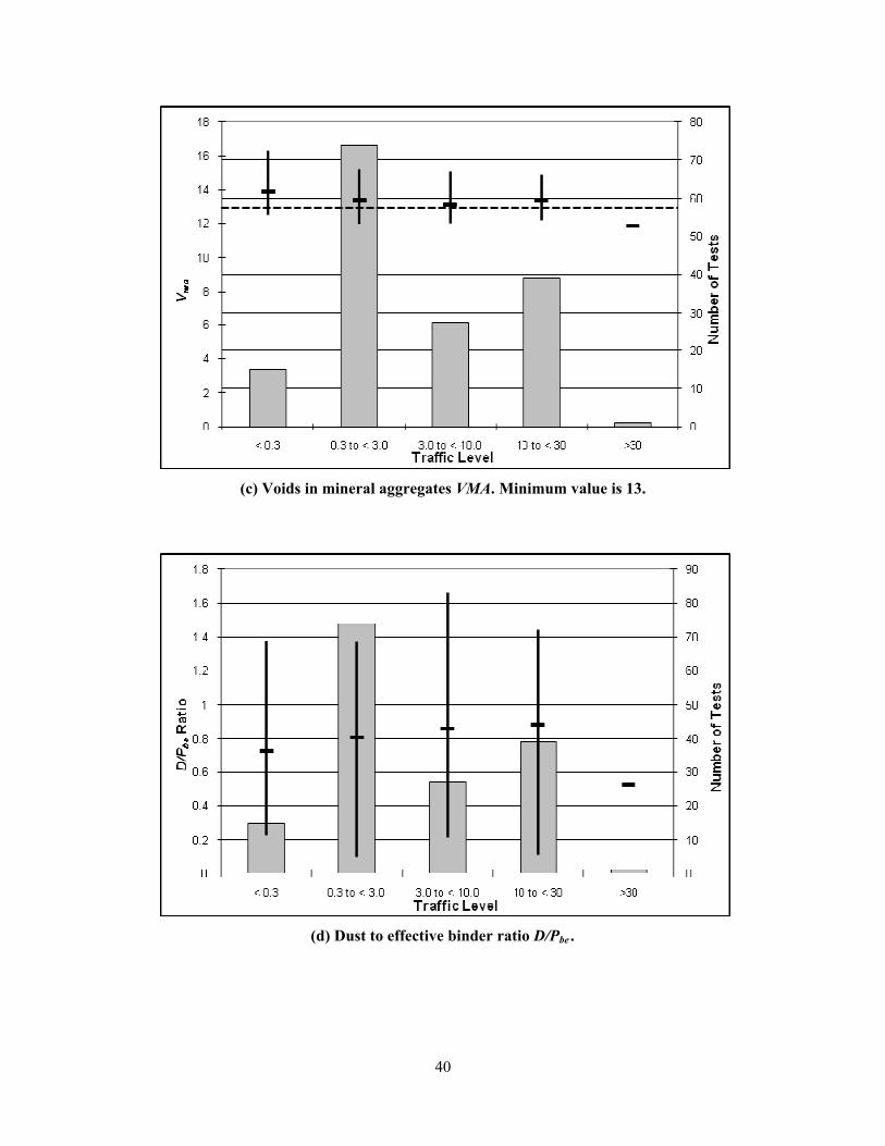
(c) Voids in mineral aggregates VMA. Minimum value is 13.

(d) Dust to effective binder ratio D/Pbe .

41

(e) Percent passing 4.75mm sieve size.

(f) Percent passing 2.36mm sieve size. Specific limits are 23 and 49.

42

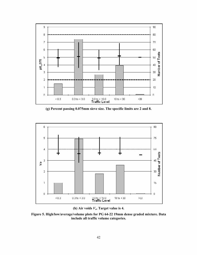
(g) Percent passing 0.075mm sieve size. The specific limits are 2 and 8.

(h) Air voids Va. Target value is 4.

Figure 5. High/low/average/volume plots for PG 64-22 19mm dense graded mixture. Data include all traffic volume categories.

43

The large amount of HMA mixture property data provided by SHA can be used to develop Maryland-specific average values for use as Level 3 inputs in the MEPDG. In order to develop these average properties, however, the appropriate level of data aggregation must be determined. Clearly, mixture gradation, and possibly volumetric properties, will be direct functions of nominal maximum aggregate size (NMAS, termed “band” in the SHA data set). Gradation and volumetric properties will also be functions of mix type (e.g., dense vs. gap graded). However, volumetric properties might also vary significantly with respect to other categorizations such as binder grade and/or traffic. Although Figure 4 and Figure 5 suggest that there were no consistent overall trends in the mean values for the gradation and volumetric properties either with regard to binder grade or traffic level, a correlation analysis was conducted to examine more thoroughly whether volumetric properties are functions of binder grade or traffic. The number of mixtures in the SHA database corresponding to each mixture type is summarized in Table 9. Since there are many different mixture types, only a representative subset was considered for the correlation analyses. These, indicated in bold italic font in Table 9, were selected to provide a range of mix size and type subsets having large numbers of data points for statistical validity. In order for the correlation results to be credible, there must be a reasonable distribution of binder grades and traffic Levels in each analysis data set. As shown in Figure 6 and Figure 7, this was achieved in most of the data sets. The results from the correlation analyses for the selected mixture types are summarized in Table 10 through Table 14. The binder grades and traffic Levels corresponding to the binder and traffic code columns are defined in Table 15. The following observations can be drawn from these results: • The volumetric properties are insensitive to binder grade. Only four correlation coefficients

were greater than 0.2. The largest coefficient was 0.47 for the correlation of binder grade and traffic for 12.5 mm mixtures. This simply reflects the fact that MDSHA uses stiffer binders for both dense and gap graded surface mixes on high volume roadways.

• The volumetric properties are insensitive to traffic Level. Eight correlation coefficients were greater than 0.2 but none exceeded 0.35.

Based on these findings, it was determined that grouping mixtures by NMAS and mix type is sufficient for determining average Level 3 input properties. A built-in query was implemented in the MatProp database to determine these average values.

44

Figure 6. Distribution of binder grades for mixture data sets in correlation analyses.

Figure 7. Distribution of traffic Levels for mixture data sets in correlation analyses.

45

Table 10. Correlation analysis result for 9.5mm high polish mixes.

BG Code Traffic CodeBG Code 1.00 Traffic Code 0.16 1.00Gmm 0.23 0.04Gmb -0.07 -0.10Gse 0.22 0.00Pb -0.12 -0.19Pba 0.09 -0.03Pbe -0.18 -0.11Va 0.11 0.12Vma 0.10 0.11Vfa -0.14 -0.15D/Pbe Ratio -0.15 0.01D/B Ratio -0.16 -0.03

Table 11. Correlation analysis result for 12.5mm virgin mixes.

BG Code Traffic CodeBG Code 1.00 Traffic Code 0.47 1.00Gmm 0.19 0.15Gmb 0.16 -0.11Gse 0.16 0.17Pb -0.20 0.00Pba -0.07 0.01Pbe -0.14 -0.01Va -0.12 0.15Vma -0.12 0.15Vfa 0.09 -0.14D/Pbe Ratio 0.02 -0.05D/B Ratio -0.07 -0.09

46

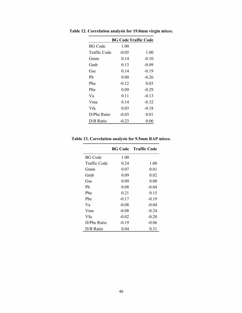
Table 12. Correlation analysis for 19.0mm virgin mixes.

BG Code Traffic CodeBG Code 1.00 Traffic Code -0.05 1.00Gmm 0.14 -0.10Gmb 0.13 -0.09Gse 0.14 -0.19Pb 0.00 -0.26Pba -0.12 0.03Pbe 0.09 -0.29Va 0.11 -0.13Vma 0.14 -0.32Vfa 0.03 -0.18D/Pbe Ratio -0.03 0.01D/B Ratio -0.23 0.06

Table 13. Correlation analysis for 9.5mm RAP mixes.

BG Code Traffic Code

BG Code 1.00 Traffic Code 0.24 1.00Gmm 0.07 0.01Gmb 0.09 0.02Gse 0.09 0.00Pb 0.08 -0.04Pba 0.21 0.15Pbe -0.17 -0.19Va -0.08 -0.04Vma -0.08 -0.24Vfa -0.02 -0.20D/Pbe Ratio -0.19 -0.06D/B Ratio 0.04 0.31

47

Table 14. Correlation analysis for 19.0mm RAP mixes.

BG Code Traffic Code

BG Code 1.00 Traffic Code 0.11 1.00Gmm 0.15 0.15Gmb 0.13 0.13Gse 0.16 0.09Pb 0.00 -0.30Pba 0.00 -0.13Pbe 0.00 -0.18Va 0.09 0.10Vma 0.06 0.00Vfa -0.01 -0.01D/Pbe Ratio 0.00 0.22D/B Ratio -0.01 0.21

Table 15. Definitions of binder and traffic codes.

Binder Code Binder Grade Traffic (MESALs)

0 PG 58-22 N/A

1 PG 58-28 <0.3

2 PG 64-22 0.3 to <3

3 PG 64-28 3 to < 10

4 PG 70-22 10 to < 30

5 PG 76-22 >30

3.3 Sensitivity Analyses for HMA Mixture Inputs

3.3.1 Level 1 vs. Level 2 vs. Level 3 Dynamic Modulus The Maryland SHA has not to date collected any Level 1 property data for any of its HMA mixtures. The SHA laboratories contain an Asphalt Mixture Performance Tester (AMPT) and a UTM-25 general purpose test system, both of which could be employed for measuring Level 1 dynamic modulus, creep compliance, and low temperature tensile strength properties. The question is whether there is a compelling reason to perform this testing. The project team recommends against Level 1 testing by SHA for creep compliance, low temperature tensile strength, and aggregate coefficient of thermal contraction. These properties

48

are used only for thermal cracking prediction, which is not a major problem in Maryland except perhaps for the western mountains in Garrett, Allegany, and Washington counties. The MEPDG generally does not predict any significant thermal cracking in Maryland provided an appropriate binder grade is specified. Given this, the Level 3 relationships built into the MEPDG code for converting dynamic modulus and other mixture properties to creep compliance, low temperature tensile strength, and aggregate coefficient of thermal contraction are judged sufficient for Maryland purposes. The recommendation for Level 1 dynamic modulus testing is different, however. Past studies using earlier versions of the MEPDG code have found significant differences in predicted performance using Level 1 vs. Level 3 dynamic modulus data (Azari et al. 2008) and some inability of Level 2/3 inputs to differentiate between different mixes adequately (e.g., Flintsch et al., 2008; Ceylan et al., 2009) The project team conducted a limited comparison analysis to confirm these general findings using the current version of the MEPDG software for Maryland conditions. The analysis scenario was a simple pavement section consisting of 10 inches of HMA (19mm dense graded, PG 76-22) over 20 inches of crushed stone base over subgrade (A-7-5). The HMA was based on the control mixture at the FHWA ALF test, which uses aggregates and binders similar to those commonly used for dense graded mixtures in Maryland. The Level 1 dynamic modulus test data was extracted from the FHWA ALF research reports. Level 3 defaults were assumed for all other material properties. Traffic was set at 950 trucks per day in the design lane and Baltimore (BWI) weather history (interpolated with DC and IAD) was taken as the climate input. Reliability was set at the MEPDG 90% default level for all distresses. The distresses predicted by the MEPDG using Level 1 vs. Level 2 vs. Level 3 dynamic modulus inputs for this scenario are summarized in Figure 8. The predicted rutting for the HMA layer is slightly larger for the Level 2 and 3 inputs than for the Level 1 value. However, the predicted total rutting using Level 2 and 3 inputs is significantly larger than when using the Level 1 inputs. Although this comparison is extremely limited (i.e., just one mixture, albeit of a type commonly used in Maryland), the findings are broadly comparable with those by others.

49

Figure 8. Comparison of predicted rutting using Level 1 vs. Level 2 vs. Level 3 HMA

dynamic modulus data.

Separate investigations by the Principal Investigator and others has consistently found that the Witczak predictive model used for Level 3 dynamic modulus inputs is dominated by temperature influences and does not do a good job of ranking mixtures in terms of their measured stiffness values at a given temperature and loading frequency (Ceylan et al. 2009). In addition, the databases used to develop and calibrate the Witczak and other similar dynamic modulus predictive models contain very few gap graded SMA mixtures of the type commonly used on high volume roads in Maryland. Given all of these issues, the project team recommends that SHA begin a program of measuring Level 1 dynamic modulus data for its more commonly used mixtures. It is envisioned that this could be done as part of the project design and/or quality assurance activities. The testing, which could be done in-house in the SHA laboratories or outsourced to commercial and/or University testing facilities, should focus on larger and/or more important projects employing mixtures having the largest tonnage production in Maryland or being placed on the highest traffic volume roadways. If this type of testing regimen were adopted as routine for large/important paving projects, SHA could amass a large body of Maryland specific Level 1 dynamic modulus data in a relatively short period of time. Note that this recommendation for Level 1 dynamic modulus testing of the HMA mixture implicitly includes Level 1 testing of the binder as well. Although it was previously concluded in Chapter 2 that Level 3 vs. Level 1/2 binder property data had little effect on predicted performance (when coupled with Level 2/3 predicted dynamic modulus), Level 1 stiffness data for the binder must be entered into the MEDPG if Level 1 dynamic modulus data is entered for the mixture. The Level 1 binder data is used by the global aging model in the MEPDG along with the Level 1 mixture data.

AC Rutting Ttl RuttingLv3 0.147 0.406Lv2_6267 0.16 0.423Lv1_6267 0.119 0.234

0

0.05

0.1

0.15

0.2

0.25

0.3

0.35

0.4

0.45

Lv3

Lv2_6267

Lv1_6267

50

3.3.2 Thermal Properties The MEPDG requires input values for the HMA thermal conductivity, heat capacity and the surface shortwave absorptivity (SSA). HMA thermal conductivity is the capability of HMA material to transmit heat, heat capacity is the capability of a HMA material to store heat, and SSA is the capability of HMA surface to absorb solar thermal radiation. These HMA thermal properties are expected to have significant effects on pavement performance. These properties are not commonly measured in the laboratory, and literature data on typical values are sparse. The MEPDG recommends values in the range of about 0.4 to 0.8 BTU/hr-ft-oF for HMA thermal conductivity, 0.2 to 0.4 BTU/lb-oF for HMA heat capacity, and 0.8 to 1.0 (dimensionless) for SSA. The basis for these recommended ranges is not known, but the ranges are reasonably narrow. In order to evaluate whether more effort needs to be devoted to better quantify these properties, a limited sensitivity study was conducted to evaluate the impact of HMA thermal conductivity and heat capacity on pavement performance (Schwartz and Li, 2010). Typical pavement sections were evaluated for College Park MD climate conditions as well as for Seattle WA, Caribou ME, and Phoenix AZ in order to evaluate more extreme climate cases. Sensitivity of performance to material inputs was quantified using the following normalized index Sji

j iRji

i jR

D XSX D

⎛ ⎞∂= ⎜ ⎟⎜ ⎟∂ ⎝ ⎠ (1)

which quantifies the variation of distress magnitude Dj about some baseline reference condition DjR cause by varying an analysis input Xi around its reference condition XiR. The normalized sensitivity index Sji can be interpreted as the percentage change in distress Dj caused by a given percentage change in input Xi. Figure 9 provides an overall summary of the normalized sensitivity indices as averaged (in absolute value terms) across all distresses. As shown, SSA has nearly the same normalized influence on overall performance at all four sites as does subgrade stiffness—i.e., a very high sensitivity. However, the normalized sensitivity indices for HMA thermal conductivity and heat capacity are about an order of magnitude lower than those for SSA.

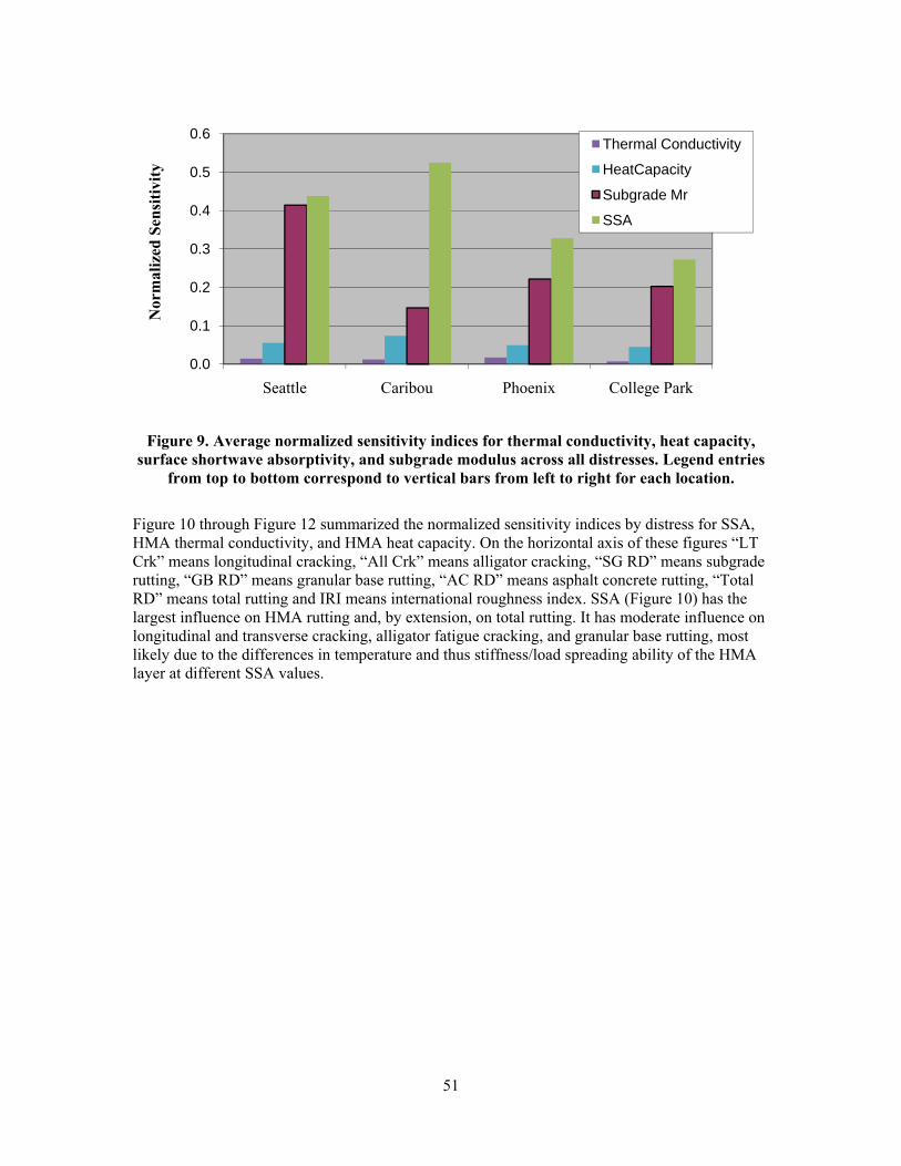
51

Figure 9. Average normalized sensitivity indices for thermal conductivity, heat capacity,

surface shortwave absorptivity, and subgrade modulus across all distresses. Legend entries from top to bottom correspond to vertical bars from left to right for each location.

Figure 10 through Figure 12 summarized the normalized sensitivity indices by distress for SSA, HMA thermal conductivity, and HMA heat capacity. On the horizontal axis of these figures “LT Crk” means longitudinal cracking, “All Crk” means alligator cracking, “SG RD” means subgrade rutting, “GB RD” means granular base rutting, “AC RD” means asphalt concrete rutting, “Total RD” means total rutting and IRI means international roughness index. SSA (Figure 10) has the largest influence on HMA rutting and, by extension, on total rutting. It has moderate influence on longitudinal and transverse cracking, alligator fatigue cracking, and granular base rutting, most likely due to the differences in temperature and thus stiffness/load spreading ability of the HMA layer at different SSA values.

0.0

0.1

0.2

0.3

0.4

0.5

0.6

Seattle Caribou Phoenix College Park

Nor

mal

ized

Sen

sitiv

ityThermal Conductivity

HeatCapacity

Subgrade Mr

SSA

52

Figure 10. Normalized sensitivity indices by distress for SSA. Legend entries from top to

bottom correspond to vertical bars from left to right for each location.

HMA thermal conductivity (Figure 11) has a negligible influence on all distresses. HMA heat capacity (Figure 12) also has a small but somewhat larger influence. Interestingly, the largest effect of heat capacity is on subgrade and base rutting, with rutting in these materials decreasing as HMA heat capacity increases. The mechanism for this is unclear. Increased heat capacity increases the thermal inertia of the HMA layer and thus smoothes out some of the temperature fluctuations in the layers, which may play a role in reducing the rutting in the unbound layers.

0.0

0.2

0.4

0.6

0.8

1.0

1.2

1.4

1.6

1.8

LT Crk All Crk SG RD GB RD AC RD Total RD IRI

Nor

mal

ized

Sen

sitiv

ity

Distress

Surface Shortwave Absorptivity

SeattleCollege ParkCaribouPhoenixOlympia

53

Figure 11. Normalized sensitivity indices by distress for thermal conductivity. Legend

entries from top to bottom correspond to vertical bars from left to right for each distress.

Figure 12. Normalized sensitivity indices by heat capacity. Legend entries from top to

bottom correspond to vertical bars from left to right for each distress.

The overall conclusion that SSA is the only environment-related HMA material input showing a strong impact on predicted performance. HMA thermal conductivity and heat capacity all show normalized sensitivity indices (averaged across all distresses in absolute value terms) an order of magnitude lower than SSA. SSA is not an easily measured parameter, however, and it changes

-0.6

-0.4

-0.2

0.0

0.2

0.4

0.6

LT Crk All Crk SG RD GB RD AC RD Total RD IRI

Nor

mal

ized

Sen

sitiv

ity

Distress

Thermal Conductivity

SeattleCollege ParkCaribouPhoenix

-0.6

-0.4

-0.2

0.0

0.2

0.4

0.6

LT Crk All Crk SG RD GB RD AC RD Total RD IRI

Nor

mal

ized

Sen

sitiv

ity

Distress

Heat Capacity

SeattleCollege ParkCaribouPhoenix

54

significantly over the pavement life (e.g., as the asphalt surface bleaches and lightens with time). Consequently, there is no good alternative to using the MEPDG Level 3 default values for this input. 3.4 Summary

3.4.1 Testing Recommendations The principal findings and recommendations relevant to HMA material property testing by SHA are as follows: 1. The HMA mixture information provided by SHA is limited to volumetric and gradation data

suitable for Level 3 input to the MEPDG. No measured dynamic modulus values suitable for Level 1 inputs are available. There is the potential for significant differences in predicted performance using Level 1 vs. Level 2/3 dynamic modulus data. In addition, the Witczak predictive equation used to generate the Level 2/3 dynamic modulus data is not intended for SMA mixtures, a common premium mixture type in Maryland, and often does not differentiate among different dense graded mixtures adequately. Therefore, SHA should plan to begin measuring Level 1 dynamic modulus data over time for the most commonly used mixture types in conjunction with major paving projects. Level 1 dynamic modulus testing of HMA mixtures will also require companion Level 1 characterization of the asphalt binders. It is recommended that SHA develop a policy requiring Level 1 HMA dynamic modulus and binder characterization testing for all major projects. Major projects could be defined by SHA in terms of a minimum placement tonnage, minimum traffic volume, or some other measure of project/mix importance. This testing could be done in-house using either the UTM-25 or AMPT test systems in the SHA laboratories; however, some equipment repair and/or calibration would be required as both of these systems are currently nonoperational. This testing could also be outsourced to local commercial testing facilities (e.g., Advanced Asphalt Technologies, LLC) and/or the University of Maryland (HMA dynamic modulus testing only).

2. There is no perceived need for measuring Level 1 creep compliance, low temperature tensile strength, and aggregate coefficient of thermal contraction properties. These properties are used only for predictions of thermal cracking, which is not a major distress type in Maryland. The Level 3 relationships built into the MEPDG code for converting dynamic modulus and other mixture inputs to creep compliance, low temperature tensile strength, and aggregate coefficient of thermal contraction are judged as sufficient for Maryland purposes.

3. HMA thermal conductivity and heat capacity generally have a very slight influence on

pavement performance predicted by the MEPDG. Consequently, the Level 3 default values built into the MEPDG software are sufficient and laboratory measurement of these properties is not warranted.

4. Although SSA has a much more significant influence on predicted performance, there at present is no easy widely-used method for measuring this parameter, either initially after construction or over the pavement life. Therefore, the Level 3 defaults values built into the MEPDG software should be used.

55

3.4.2 Recommended MEPDG Inputs The recommended HMA dynamic modulus and asphalt inputs to the MEPDG for Maryland conditions are summarized in Table 16 and Table 17 for new and existing HMA layers, respectively. Table 18 summarizes the recommendations for creep compliance and low temperature tensile strength inputs for both new and exiting HMA layers.

Table 16. Recommendation material property inputs for new HMA layers for Maryland conditions.

Property Input Level

Value Comment

Asphalt material type All Asphalt concrete Only option available. Layer thickness All Project specific Asphalt Mix Dynamic Modulus Table 1 Mixture specific Recommended for future collection. Aggregate gradation and volumetric properties1

2/3 Mixture specific See Table 19 for typical values for Maryland mixtures.

Asphalt Binder Superpave binder dynamic stiffness data

1/2 Binder specific Recommended for future collection.

Superpave binder grade 3 Mixture specific See Table 4 for Maryland SHA binder recommendations.

Asphalt General Reference temperature All 70 Does not influence predictions. Effective binder content All Mixture specific See Table 19 for typical values for Maryland

mixtures. In-Place Air Voids All Project specific See Table 19 for typical values for Maryland

mixtures. Total unit weight All Project specific See Table 20 for typical values for Maryland

mixtures. (Note: Values in table should be adjusted for in-place air voids percentage.)

Poisson’s ratio All 0.35 MEPDG default Thermal conductivity All 0.67 MEPDG default (global calibration value). Heat capacity asphalt All 0.23 MEPDG default (global calibration value). Short wave absorption All 0.85 MEPDG default (global calibration value). 1Percent retained above the 3/4” sieve; percent retained above the 3/8” sieve; percent retained above the #4 sieve; percent passing the #200 sieve; effective volumetric binder content (%); and in-place air voids (%).

56

Table 17. Recommendation material property inputs for existing HMA layers for Maryland conditions.

Property Input Level

Value Comment

Asphalt material type All Asphalt concrete Layer thickness All Project specific Asphalt Mix Aggregate gradation and volumetric properties1

All Mixture specific See Table 19 for typical values for Maryland mixtures.

Superpave binder dynamic stiffness data

1/2 Binder specific Recommended for future collection.

Superpave binder grade 3 Mixture specific See Table 4 for Maryland SHA binder recommendations.

Asphalt General Reference temperature All 70 Does not influence predictions. Effective binder content All Mixture specific See Table 19 for typical values for Maryland

mixtures. In-Place Air Voids All Project specific See Table 19 for typical values for Maryland

mixtures. Total unit weight All Project specific Poisson’s ratio All 0.35 MEPDG default Thermal conductivity All 0.67 MEPDG default (global calibration value). Heat capacity asphalt All 0.23 MEPDG default (global calibration value). Pavement condition rating

All Project specific

1Percent retained above the 3/4” sieve; percent retained above the 3/8” sieve; percent retained above the #4 sieve; percent passing the #200 sieve; effective volumetric binder content (%); and in-place air voids (%).

Table 18. Recommendation thermal cracking inputs for new HMA layers for Maryland conditions.

Property Input Level

Value Comment

Average tensile strength at 14 ºC 3 Mixture specific MEPDG calculated value Creep compliance 3 Mixture specific MEPDG calculated value Mixture coefficient of thermal contraction 3 Mixture specific MEPDG calculated value Aggregate coefficient of thermal contraction 3 Project specific See Table 6

57

Table 19. Level 3 inputs for Maryland HMA mixtures (based on material properties database at time of report).

NMAS (mm) Mix Type

% Retained above

3/4” sieve

% Retained above

3/8” sieve

% Retained above

#4 sieve

% Passing #200 sieve

Effective Volumetric Binder

Content (%)

In-Place Air Voids

(%) 4.75 Virgin 0.0  0.0  6.9  7.7  14.06 6.54 9.5 Shingle 0.0  4.8  39.2  6.4  11.61 6.47 9.5 RAP 0.0  4.7  38.1  5.5  11.59 6.47 9.5 Virgin 0.0  3.7  34.5  6.0  11.88 6.47 9.5 GAP 0.0  10.7  61.3  9.2  14.85 6.47 9.5 High Polish 0.0  3.4  36.7  5.5  11.76 6.47

12.5 High Polish 0.0  14.0  49.1  5.1  11.09 6.47 12.5 RAP 0.0  13.0  50.0  5.4  10.70 6.47 12.5 Shingle 0.0  14.2  50.7  6.1  10.73 6.47 12.5 Virgin 0.0  15.6  45.3  5.3  11.14 6.47 12.5 GAP 0.0  21.7  66.8  8.6  14.31 6.47 19 GAP 5.0  44.0  74.0  8.1  13.84 6.47 19 RAP 3.5  26.6  57.4  5.0  9.69 6.47 19 Shingle 4.1  29.5  58.8  5.6  9.72 6.47 19 High Polish 2.5  30.4  58.3  5.3  10.20 6.47 19 Virgin 5.5  33.5  55.5  4.9  10.08 6.47 25 RAP 11.7  40.6  65.2  4.7  9.10 6.47 25 Virgin 15.0  47.0  63.5  4.2  9.46 6.47

37.5 RAP 23.0  52.2  70.8  4.4  8.38 6.47 4.75 Virgin 0.0  0.0  6.9  7.7  14.06 6.54

Table 20. SHA historical unit weights for Superpave mixes at 4% air voids (OMT, 2006).

59

4. PCC DATA 4.1 MEPDG Input Requirements 4.1.1 New Construction/Reconstruction/Overlays The key project-specific PCC stiffness and strength properties required for new construction/reconstruction/overlay designs in the MEPDG are the elastic modulus (Ec) and the modulus of rupture (MOR). The methods for determining these properties at each of the input levels in the MEPDG are summarized in Table 21 and Table 22. The corresponding required user inputs at each level are:

• Level 1: Ec and MOR at 7, 14, 28, and 90 days and the estimated ratio of 20 year to 28 day values.

• Level 2: Compressive strength (fc′) at 7, 14, 28 and 90 days and the estimated ratio of 20 year to 28 day values. The corresponding Ec and MOR values are estimated using the standard empirical relationships shown in Table 21 and Table 22.

• Level 3: Either the 28-day MOR or the 28-day fc′. The corresponding 28-day Ec modulus is then either estimated by the MEPDG software using the standard empirical relationship shown in Table 21 or optionally provided by the user. The values of Ec and MOR are determined at other time values using the default aging relationships shown in Table 21 and Table 22, respectively.

Additional PCC properties required at all input levels include:

• Mix properties: Unit weight; Poisson’s ratio; cement type; cementitious material content; water cement ratio; aggregate type; curing method.

• Thermal properties: thermal conductivity; heat capacity; surface shortwave absorptivity; coefficient of thermal expansion; PCC zero-stress temperature

• Shrinkage properties: ultimate shrinkage at 40% relative humidity; reversible shrinkage; time to develop 50% of ultimate shrinkage.

The methods for determining thermal conductivity, heat capacity, and surface shortwave absorptivity at each of the input levels in the MEPDG are summarized in Table 23. Coefficient of thermal expansion can be measured using AASHTO TP60 (Level 1), approximated using mixture theory (Level 2), or estimated from historical values (Level 3). Default values are provided in the MEPDG software for all of these additional PCC properties. These default values may be overridden by the user if desired.

60

Table 21. PCC elastic modulus estimation for new, reconstruction, and overlay design (NCHRP, 2004).

61

Table 22. PCC modulus of rupture estimation for new or reconstruction design and PCC overlay design (NCHRP, 2004).

62

Table 23. Estimation of PCC thermal conductivity, heat capacity, and surface absorptivity at various hierarchical input levels (NCHRP, 2004).

4.1.2 Rehabilitation There are two primary differences between characterizing new concrete layers and existing layers: (a) the Ec and MOR values for existing PCC slabs to be overlaid need to be adjusted for the damage caused to the pavement by traffic loads and environmental effects; (b) gains in Ec and MOR over time are not considered for the old existing PCC. The material properties required by the MEPDG at each input level for existing PCC in rehabilitation projects are as follows:

• Level 1: o Elastic modulus ETEST is measured from cores taken from the existing pavement

in accordance with ASTM C 46. Alternatively, ETEST can be determined via FWD nondestructive evaluation at mid-slab. ETEST is then adjusted for pavement condition to determine the Ec value of the existing pavement to be used in design:

c TESTE C E= ∗ (2) in which C is the pavement condition factor given in Table 24.

o In-place MOR is measured from prismatic beams cut from the existing concrete pavement in accordance with AASHTO T97.

• Level 2: o In-place fc′ is measured from cores taken from the existing pavement in

accordance with AASHTO T22.

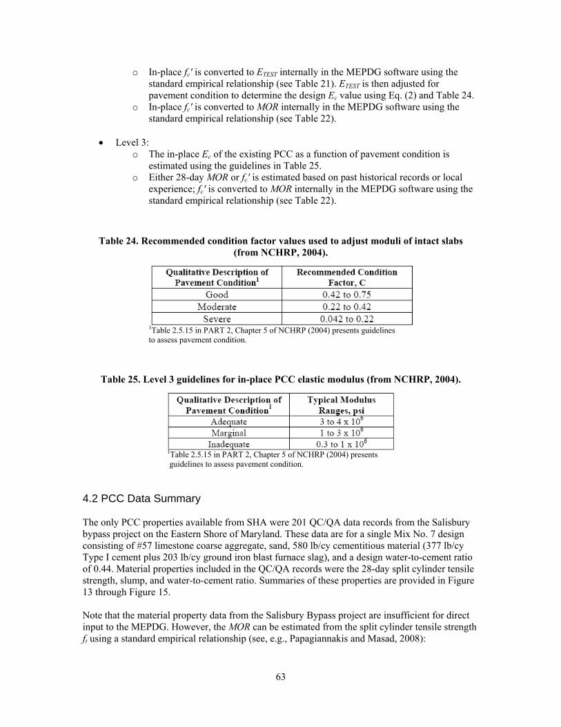
63

o In-place fc′ is converted to ETEST internally in the MEPDG software using the standard empirical relationship (see Table 21). ETEST is then adjusted for pavement condition to determine the design Ec value using Eq. (2) and Table 24.

o In-place fc′ is converted to MOR internally in the MEPDG software using the standard empirical relationship (see Table 22).

• Level 3: o The in-place Ec of the existing PCC as a function of pavement condition is

estimated using the guidelines in Table 25. o Either 28-day MOR or fc′ is estimated based on past historical records or local

experience; fc′ is converted to MOR internally in the MEPDG software using the standard empirical relationship (see Table 22).

Table 24. Recommended condition factor values used to adjust moduli of intact slabs (from NCHRP, 2004).

1Table 2.5.15 in PART 2, Chapter 5 of NCHRP (2004) presents guidelines

to assess pavement condition.

Table 25. Level 3 guidelines for in-place PCC elastic modulus (from NCHRP, 2004).

1Table 2.5.15 in PART 2, Chapter 5 of NCHRP (2004) presents

guidelines to assess pavement condition.

4.2 PCC Data Summary The only PCC properties available from SHA were 201 QC/QA data records from the Salisbury bypass project on the Eastern Shore of Maryland. These data are for a single Mix No. 7 design consisting of #57 limestone coarse aggregate, sand, 580 lb/cy cementitious material (377 lb/cy Type I cement plus 203 lb/cy ground iron blast furnace slag), and a design water-to-cement ratio of 0.44. Material properties included in the QC/QA records were the 28-day split cylinder tensile strength, slump, and water-to-cement ratio. Summaries of these properties are provided in Figure 13 through Figure 15. Note that the material property data from the Salisbury Bypass project are insufficient for direct input to the MEPDG. However, the MOR can be estimated from the split cylinder tensile strength ft using a standard empirical relationship (see, e.g., Papagiannakis and Masad, 2008):

64

1.35 tMOR f= (3) Using this relation and the data in Figure 13, the average MOR for the Salisbury bypass mix is estimated at 685 psi.

Figure 13. Summary of split cylinder tensile strength data provided by SHA.

Figure 14. Summary of slump data provided by SHA.

2 2

11

15 14

28

20

23 23

28

17

11

42 1

0

5

10

15

20

25

30

380  400  420  440  460  480  500  520  540  560  580  600  620  640  660 

Freq

uency

Split Cylinder Tensile Strength (psi)

Mean: 507.7StDev: 57.04

211

27

92

38

114 2 1 0 1 3 0 3 2 3 0 0 0 1

0

10

20

30

40

50

60

70

80

90

100

0.25 0.5

0.75

1

1.25 1.5

1.75

2

2.25 2.5

2.75

3

3.25 3.5

3.75

4

4.25 4.5

4.75

5

Freq

uency

Slump (in)

Mean: 1.21StDev: 0.71

65

Figure 15. Summary of water-to-cement ratio data provided by SHA.

4.3 Sensitivity Analyses for PCC Inputs

4.3.1 Strength and Stiffness Properties Effect of Input Level  The major question regarding the appropriate input level for PCC strength and stiffness data is: “Are there significant differences in predicted performance from the MEPDG using Level 1, 2 or 3 PCC material inputs?” A review of the literature found a few relevant studies, but they either did not definitively address the question or they were for climate conditions significantly different from Maryland. Therefore, the project team conducted a very limited comparison of MEPDG predictions using Level 1 vs. Level 2 vs. Level 3 PCC inputs for typical Maryland conditions. Since no Level 1 PCC material properties were available from SHA, the project team tried several alternatives to obtain the required data. In the first attempt, 28-day PCC compressive strength, 28-day modulus of rupture, and 28-day elastic modulus data collected by the University of Maryland as part of the Salisbury bypass project were used along with the property vs. time relations incorporated in the MEPDG to estimate the missing Level 1 and Level 2 PCC properties. No significant differences were found among the Level 1, 2, and 3 predicted performances. However, this was expected and merely shows that PCC material inputs portion of the MEPDG software is bug-free and internally consistent. The second attempt capitalized on a study by Hall and Beam (2005) that detailed Level 1, 2 and 3 PCC property data for a specific concrete mixture. Using these data, the MEPDG predicted

2 40

16 16

60 59

22

148

0

10

20

30

40

50

60

70

0.32  0.34  0.36  0.38  0.4  0.42  0.44  0.46  0.48  0.5 

Freq

uency

Water‐to‐Cement Ratio

Mean: 0.43StDev: 0.03 

66

performance again showed little difference between Level 1, Level 2, and Level 3 inputs. However, the Hall and Beam paper did not describe how the Level 2 and Level 3 data were obtained. It is quite likely that these data were generated using the same approach as our initial attempt with the Salisbury bypass data. The third and best attempt was based on measured Level 1, 2, and 3 PCC material input data acquired from Missouri DOT for five PCC mixes (ARA, 2009). All five mixes used Type I cement, limestone coarse aggregate, and flyash1. The mix composition data are described in Table 26 and the corresponding measured stiffness and strength data are summarized in Table 27. Plots of Ec and MOR are shown in Figure 16 and Figure 17. The Ec and MOR values when normalized by their 28-day values are replotted in Figure 18 and Figure 19 along with the MEPDG Level 3 default strength and stiffness gains. Note that although these are the best PCC material property data that could be found by the project team, there are still some anomalies:

• high 14-day Ec and MOR values (or alternatively a counterintuitive dip in the 28-day Ec and MOR values) for the Gradation B mixture;

• an elevated 7-day MOR for the Gradation B Opt mixture at 7 days; • anomalously high 28-day Ec and MOR values and/or anomalously low 90-day values for

the Gradation D Opt mixture; • consistently higher MOR values for Gradation F as compared to the other mixtures at all

ages but particularly at 90 days; • measured stiffness and strength changes with time (Figure 18 and Figure 19) that are

greater than those predicted by the MEPDG Level 3 default aging relations (with the exception of the Gradation D Opt mixture, but this may be because of the anomalously high 28-day Ec and MOR values used to normalize the trends).

Table 26. Composition of Missouri DOT PCC mixes (ARA, 2009).

1 Flyash affects the rate of strength gain.

67

Table 27. Mixture Properties from Missouri DOT.

MoDOT Mix Designation

Sample Age, days

Compressive Strength, psi

Flexural Strength (MOR), psi

Modulus of Elasticity, psi

Gradation B

3 3343 477 3775772 7 4001 550 4172195

14 4390 654 4318238 28 4902 626 4290195 90 5421 674 4757531

Gradation B Opt

3 3472 564 3729516 7 3936 634 3972549

14 4474 652 4164558 28 4857 718 4266237 90 5606 788 4632843

Gradation D

3 3756 587 3835707 7 4472 595 4291245

14 4848 640 4271614 28 5082 655 4452082 90 5875 725 4974852

Gradation D Opt

3 3884 540 4049615 7 4382 583 4239712

14 4810 637 4347735 28 5120 744 4958388 90 5970 699 4785520

Gradation F

3 3243 566 3348184 7 3847 654 3767819*

14 4502 739 4101783 28 4886 772 4320960 90 5643 897 4635612

*Missing data; interpolated via regression analysis from other Gradation F Ec values.

68

Figure 16. Measured Ec for Missouri PCC mixes.

Figure 17. Measured MOR for Missouri PCC mixes.

3000000

3500000

4000000

4500000

5000000

5500000

0 20 40 60 80 100

E c(psi)

Age (days)

B

B Opt

D

D Opt

F

400

500

600

700

800

900

1000

0 20 40 60 80 100

MOR (psi)

Age (days)

B

B Opt

D

D Opt

F

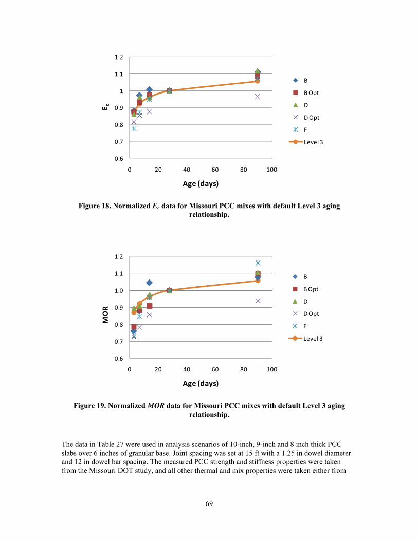
69

Figure 18. Normalized Ec data for Missouri PCC mixes with default Level 3 aging

relationship.

Figure 19. Normalized MOR data for Missouri PCC mixes with default Level 3 aging

relationship.

The data in Table 27 were used in analysis scenarios of 10-inch, 9-inch and 8 inch thick PCC slabs over 6 inches of granular base. Joint spacing was set at 15 ft with a 1.25 in dowel diameter and 12 in dowel bar spacing. The measured PCC strength and stiffness properties were taken from the Missouri DOT study, and all other thermal and mix properties were taken either from

0.6

0.7

0.8

0.9

1

1.1

1.2

0 20 40 60 80 100

E c

Age (days)

B

B Opt

D

D Opt

F

Level 3

0.6

0.7

0.8

0.9

1.0

1.1

1.2

0 20 40 60 80 100

MOR

Age (days)

B

B Opt

D

D Opt

F

Level 3

70

the Maryland Salisbury bypass project or set equal to the MEPDG Level 3 defaults.2 Initial two-way AADTT was set at 4000 (Principal Arterials – Interstate and Defense, TTC 1), with all other traffic variables set equal to the Level 3 default values in MEPDG. Baltimore (BWI) weather history was interpolated with Washington Dulles (IAD) data for the climate input to the MEPDG. This interpolation was required because the BWI weather history has gaps. The MEPDG default reliability of 90% was used for all predicted distresses. The distresses predicted by the MEPDG using Level 1, 2 and 3 inputs for these scenarios are summarized in Table 28 to Table 32. Each table corresponds to one set of mix properties in Table 27 as applied to each of the three slab thicknesses (only the 8 inch slab thickness was analyzed for Gradation F because of the small levels of cracking predicted). The four alternatives for Level 3 are: Level 3a – 28-day fc′ only; Level 3b – 28-day MOR only; Level 3c – 28-day fc′ and Ec; and Level 3d – 28-day MOR and Ec. The Missouri DOT report did not specify the estimated 20-year to 28-day property ratio. Therefore the Level 3 default value of 1.2 was used.

2 CTE values were measured for the Missouri mixes, but these data are judged to be unreliable.

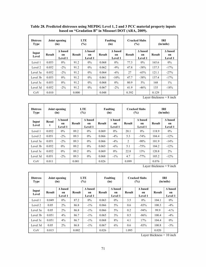
71

Table 28. Predicted distresses using MEPDG Level 1, 2 and 3 PCC material property inputs based on “Gradation B” in Missouri DOT (ARA, 2009).

Distress Type

Joint opening (in)

LTE (%)

Faulting (in)

Cracked Slabs (%)

IRI (in/mile)

Input Level Result

Δ based on

Level 1 Result

Δ based on

Level 1 Result

Δ based on

Level 1 Result

Δ based on

Level 1 Result

Δ based on

Level 1 Level 1 0.053 0% 91.2 0% 0.068 0% 77.3 0% 165.6 0%

Level 2 0.052 -2% 91.2 0% 0.062 -9% 47.8 -38% 137.5 -17%

Level 3a 0.052 -2% 91.2 0% 0.064 -6% 27 -65% 121.1 -27%

Level 3b 0.053 0% 91.2 0% 0.061 -10% 47.7 -38% 137.4 -17%

Level 3c 0.053 0% 91.2 0% 0.068 0% 80.9 5% 168 1%

Level 3d 0.052 -2% 91.2 0% 0.067 -2% 41.9 -46% 135 -18%

CoV 0.010 0.000 0.048 0.392 0.129 Layer thickness = 8 inch

Distress Type

Joint opening (in)

LTE (%)

Faulting (in)

Cracked Slabs (%)

IRI (in/mile)

Input Level

Result

Δ based on

Level 1 Result

Δ based on

Level 1 Result

Δ based on

Level 1 Result

Δ based on

Level 1 Result

Δ based on

Level 1 Level 1 0.052 0% 89.2 0% 0.069 0% 20.1 0% 118.9 0%

Level 2 0.051 -2% 89.3 0% 0.066 -4% 5.3 -74% 104.4 -12%

Level 3a 0.051 -2% 89.3 0% 0.066 -4% 2 -90% 101.9 -14%

Level 3b 0.052 0% 89.2 0% 0.065 -6% 5.1 -75% 104.2 -12%

Level 3c 0.052 0% 89.2 0% 0.069 0% 22.8 13% 120.8 2%

Level 3d 0.051 -2% 89.3 0% 0.068 -1% 4.7 -77% 105.2 -12%

CoV 0.011 0.001 0.026 0.899 0.076 Layer thickness = 9 inch

Distress Type

Joint opening (in)

LTE (%)

Faulting (in)

Cracked Slabs (%)

IRI (in/mile)

Input Level Result

Δ based on

Level 1 Result

Δ based on

Level 1 Result

Δ based on

Level 1 Result

Δ based on

Level 1 Result

Δ based on

Level 1 Level 1 0.049 0% 87.2 0% 0.063 0% 3.5 0% 104.1 0%

Level 2 0.05 2% 86.8 -1% 0.066 5% 0.6 -83% 100.3 -4%

Level 3a 0.05 2% 86.8 -1% 0.066 5% 0.2 -94% 99.9 -4.%

Level 3b 0.051 4% 86.7 -1% 0.065 3% 0.5 -86% 100.4 -4%

Level 3c 0.051 4% 86.7 -1% 0.068 8% 4.1 17% 104.4 0%

Level 3d 0.05 2% 86.8 -1% 0.067 6% 0.6 -83% 100.8 -3%

CoV 0.015 0.002 0.026 1.095 0.020 Layer thickness = 10 inch

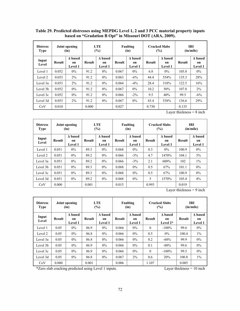
72

Table 29. Predicted distresses using MEPDG Level 1, 2 and 3 PCC material property inputs based on “Gradation B Opt” in Missouri DOT (ARA, 2009).

Distress Type

Joint opening (in)

LTE (%)

Faulting (in)

Cracked Slabs (%)

IRI (in/mile)

Input Level Result

Δ based on

Level 1 Result

Δ based on

Level 1 Result

Δ based on

Level 1 Result

Δ based on

Level 1 Result

Δ based on

Level 1 Level 1 0.052 0% 91.2 0% 0.067 0% 6.8 0% 105.8 0%

Level 2 0.053 2% 91.2 0% 0.063 -6% 44.4 554% 135.3 28%

Level 3a 0.053 2% 91.2 0% 0.064 -4% 28.4 318% 122.5 16%

Level 3b 0.052 0% 91.2 0% 0.067 0% 10.2 50% 107.8 2%

Level 3c 0.052 0% 91.2 0% 0.066 -2% 9.5 40% 99.5 -6%

Level 3d 0.053 2% 91.2 0% 0.067 0% 43.4 538% 136.6 29%

CoV 0.010 0.000 0.027 0.730 0.135 Layer thickness = 8 inch

Distress Type

Joint opening (in)

LTE (%)

Faulting (in)

Cracked Slabs (%)

IRI (in/mile)

Input Level Result

Δ based on

Level 1 Result

Δ based on

Level 1 Result

Δ based on

Level 1 Result

Δ based on

Level 1 Result

Δ based on

Level 1 Level 1 0.051 0% 89.3 0% 0.068 0% 0.3 0% 100.9 0%

Level 2 0.051 0% 89.2 0% 0.066 -3% 4.7 1470% 104.1 3%

Level 3a 0.051 0% 89.2 0% 0.066 -3% 2.1 600% 102 1%

Level 3b 0.051 0% 89.3 0% 0.068 0% 0.5 67% 101.1 0%

Level 3c 0.051 0% 89.3 0% 0.068 0% 0.5 67% 100.9 0%

Level 3d 0.051 0% 89.2 0% 0.068 0% 5 1570% 105.4 4%

CoV 0.000 0.001 0.015 0.993 0.019 Layer thickness = 9 inch

Distress Type

Joint opening (in)

LTE (%)

Faulting (in)

Cracked Slabs (%)

IRI (in/mile)

Input Level Result

Δ based on

Level 1 Result

Δ based on

Level 1 Result

Δ based on

Level 1 Result

Δ based on

Level 2* Result

Δ based on

Level 1 Level 1 0.05 0% 86.9 0% 0.066 0% 0 -100% 99.6 0%

Level 2 0.05 0% 86.8 0% 0.066 0% 0.5 0% 100.4 1%

Level 3a 0.05 0% 86.8 0% 0.066 0% 0.2 -60% 99.9 0%

Level 3b 0.05 0% 86.9 0% 0.066 0% 0.1 -80% 99.6 0%

Level 3c 0.05 0% 86.9 0% 0.066 0% 0 -100% 99.5 0%

Level 3d 0.05 0% 86.8 0% 0.067 2% 0.6 20% 100.8 1%

CoV 0.000 0.001 0.006 1.107 0.005 *Zero slab cracking predicted using Level 1 inputs. Layer thickness = 10 inch

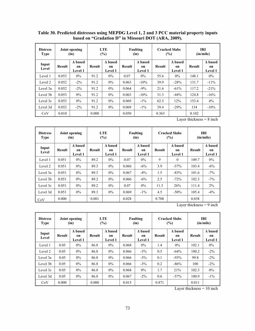
73

Table 30. Predicted distresses using MEPDG Level 1, 2 and 3 PCC material property inputs based on “Gradation D” in Missouri DOT (ARA, 2009).

Distress Type

Joint opening (in)

LTE (%)

Faulting (in)

Cracked Slabs (%)

IRI (in/mile)

Input Level Result

Δ based on

Level 1 Result

Δ based on

Level 1 Result

Δ based on

Level 1 Result

Δ based on

Level 1 Result

Δ based on

Level 1 Level 1 0.053 0% 91.2 0% 0.07 0% 55.6 0% 148.1 0%

Level 2 0.052 -2% 91.2 0% 0.063 -10% 39.9 -28% 131.7 -11%

Level 3a 0.052 -2% 91.2 0% 0.064 -9% 21.6 -61% 117.2 -21%

Level 3b 0.053 0% 91.2 0% 0.063 -10% 31.3 -44% 124.8 -16%

Level 3c 0.053 0% 91.2 0% 0.069 -1% 62.5 12% 153.4 4%

Level 3d 0.052 -2% 91.2 0% 0.069 -1% 39.4 -29% 134 -10%

CoV 0.010 0.000 0.050 0.363 0.102 Layer thickness = 8 inch

Distress Type

Joint opening (in)

LTE (%)

Faulting (in)

Cracked Slabs (%)

IRI (in/mile)

Input Level Result

Δ based on

Level 1 Result

Δ based on

Level 1 Result

Δ based on

Level 1 Result

Δ based on

Level 1 Result

Δ based on

Level 1 Level 1 0.051 0% 89.2 0% 0.07 0% 9 0 109.7 0%

Level 2 0.051 0% 89.3 0% 0.066 -6% 3.9 -57% 103.4 -6%

Level 3a 0.051 0% 89.3 0% 0.067 -4% 1.5 -83% 101.6 -7%

Level 3b 0.051 0% 89.2 0% 0.066 -6% 2.5 -72% 102.3 -7%

Level 3c 0.051 0% 89.2 0% 0.07 0% 11.3 26% 111.4 2%

Level 3d 0.051 0% 89.3 0% 0.069 -1% 4.5 -50% 105.4 -4%

CoV 0.000 0.001 0.028 0.708 0.038

Layer thickness = 9 inch

Distress Type

Joint opening (in)

LTE (%)

Faulting (in)

Cracked Slabs (%)

IRI (in/mile)

Input Level Result

Δ based on

Level 1 Result

Δ based on

Level 1 Result

Δ based on

Level 1 Result

Δ based on

Level 1 Result

Δ based on

Level 1 Level 1 0.05 0% 86.8 0% 0.068 0% 1.4 0% 102.1 0%

Level 2 0.05 0% 86.8 0% 0.066 -3% 0.5 -64% 100.2 -2%

Level 3a 0.05 0% 86.8 0% 0.066 -3% 0.1 -93% 99.8 -2%

Level 3b 0.05 0% 86.8 0% 0.066 -3% 0.2 -86% 100 -2%

Level 3c 0.05 0% 86.8 0% 0.068 0% 1.7 21% 102.3 0%

Level 3d 0.05 0% 86.8 0% 0.067 -2% 0.6 -57% 100.9 -1%

CoV 0.000 0.000 0.015 0.871 0.011 Layer thickness = 10 inch

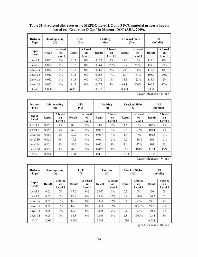
74

Table 31. Predicted distresses using MEPDG Level 1, 2 and 3 PCC material property inputs based on “Gradation D Opt” in Missouri DOT (ARA, 2009).

Distress Type

Joint opening (in)

LTE (%)

Faulting (in)

Cracked Slabs (%)

IRI (in/mile)

Input Level Result

Δ based on

Level 1 Result

Δ based on

Level 1 Result

Δ based on

Level 1 Result

Δ based on

Level 1 Result

Δ based on

Level 1 Level 1 0.052 0% 91.3 0% 0.071 0% 18.5 0% 117.3 0%

Level 2 0.052 0% 91.2 0% 0.064 -20% 36.7 98% 129.3 10%

Level 3a 0.052 0% 91.2 0% 0.065 -8% 21 14% 116.8 0%

Level 3b 0.052 0% 91.3 0% 0.068 -4% 6.1 -67% 105.7 -10%

Level 3c 0.052 0% 91.3 0% 0.072 1% 14.5 -22% 114.9 -2%

Level 3d 0.052 0% 91.2 0% 0.073 3% 69.1 274% 160.7 37%

CoV 0.000 0.001 0.055 0.819 0.157 Layer thickness = 8 inch

Distress Type

Joint opening (in)

LTE (%)

Faulting (in)

Cracked Slabs (%)

IRI (in/mile)

Input Level Result

Δ based on

Level 1 Result

Δ based on

Level 1 Result

Δ based on

Level 1 Result

Δ based on

Level 1 Result

Δ based on

Level 1 Level 1 0.051 0% 89.3 0% 0.07 0% 1.5 0% 102.7 0%

Level 2 0.051 0% 89.3 0% 0.067 -4% 3.4 127% 103.1 0%

Level 3a 0.051 0% 89.3 0% 0.067 -4% 1.4 -7% 101.5 -1%

Level 3b 0.051 0% 89.3 0% 0.068 -3% 0.3 -80% 101 -2%

Level 3c 0.051 0% 89.3 0% 0.071 1% 1.1 -27% 103 0%

Level 3d 0.051 0% 89.3 0% 0.072 3% 15.9 960% 116.1 13%

CoV 0.000 0.000 0.031 1.513 0.055 Layer thickness = 9 inch

Distress Type

Joint opening (in)

LTE (%)

Faulting (in)

Cracked Slabs (%)

IRI (in/mile)

Input Level Result

Δ based on

Level 1 Result

Δ based on

Level 1 Result

Δ based on

Level 1 Result

Δ based on

Level 1 Result

Δ based on

Level 1 Level 1 0.05 0% 87.0 0% 0.067 0% 0.2 0% 100 0%

Level 2 0.05 0% 86.8 0% 0.066 -2% 0.4 100% 100.2 0%

Level 3a 0.05 0% 86.8 0% 0.066 -2% 0.1 -50% 99.8 9%

Level 3b 0.05 0% 87.0 0% 0.066 -2% 0 -100.0% 99.5 -1%

Level 3c 0.05 0% 87.0 0% 0.068 2% 0.1 -50% 100.3 0%

Level 3d 0.05 0% 86.8 0% 0.069 3% 2.8 1300% 103.4 3%

CoV 0.000 0.001 0.019 1.810 0.014 Layer thickness = 10 inch

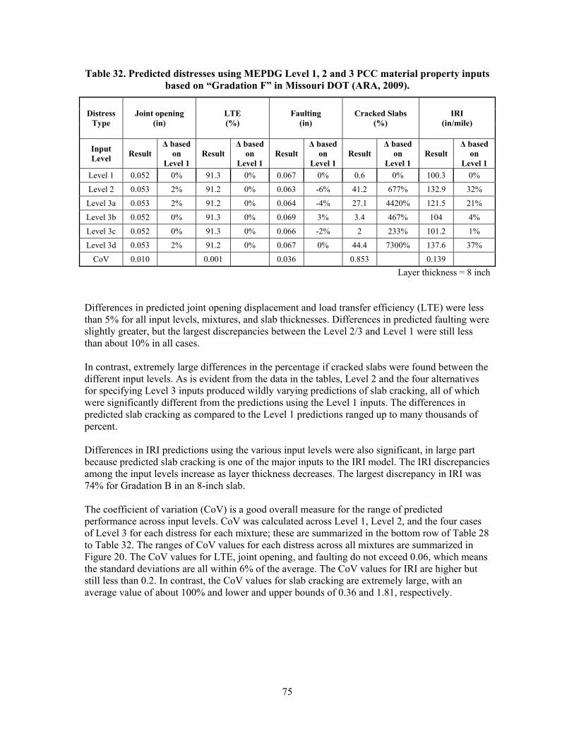
75

Table 32. Predicted distresses using MEPDG Level 1, 2 and 3 PCC material property inputs based on “Gradation F” in Missouri DOT (ARA, 2009).

Distress Type

Joint opening (in)

LTE (%)

Faulting (in)

Cracked Slabs (%)

IRI (in/mile)

Input Level Result

Δ based on

Level 1 Result

Δ based on

Level 1 Result

Δ based on

Level 1 Result

Δ based on

Level 1 Result

Δ based on

Level 1 Level 1 0.052 0% 91.3 0% 0.067 0% 0.6 0% 100.3 0%

Level 2 0.053 2% 91.2 0% 0.063 -6% 41.2 677% 132.9 32%

Level 3a 0.053 2% 91.2 0% 0.064 -4% 27.1 4420% 121.5 21%

Level 3b 0.052 0% 91.3 0% 0.069 3% 3.4 467% 104 4%

Level 3c 0.052 0% 91.3 0% 0.066 -2% 2 233% 101.2 1%

Level 3d 0.053 2% 91.2 0% 0.067 0% 44.4 7300% 137.6 37%

CoV 0.010 0.001 0.036 0.853 0.139 Layer thickness = 8 inch

Differences in predicted joint opening displacement and load transfer efficiency (LTE) were less than 5% for all input levels, mixtures, and slab thicknesses. Differences in predicted faulting were slightly greater, but the largest discrepancies between the Level 2/3 and Level 1 were still less than about 10% in all cases. In contrast, extremely large differences in the percentage if cracked slabs were found between the different input levels. As is evident from the data in the tables, Level 2 and the four alternatives for specifying Level 3 inputs produced wildly varying predictions of slab cracking, all of which were significantly different from the predictions using the Level 1 inputs. The differences in predicted slab cracking as compared to the Level 1 predictions ranged up to many thousands of percent. Differences in IRI predictions using the various input levels were also significant, in large part because predicted slab cracking is one of the major inputs to the IRI model. The IRI discrepancies among the input levels increase as layer thickness decreases. The largest discrepancy in IRI was 74% for Gradation B in an 8-inch slab. The coefficient of variation (CoV) is a good overall measure for the range of predicted performance across input levels. CoV was calculated across Level 1, Level 2, and the four cases of Level 3 for each distress for each mixture; these are summarized in the bottom row of Table 28 to Table 32. The ranges of CoV values for each distress across all mixtures are summarized in Figure 20. The CoV values for LTE, joint opening, and faulting do not exceed 0.06, which means the standard deviations are all within 6% of the average. The CoV values for IRI are higher but still less than 0.2. In contrast, the CoV values for slab cracking are extremely large, with an average value of about 100% and lower and upper bounds of 0.36 and 1.81, respectively.

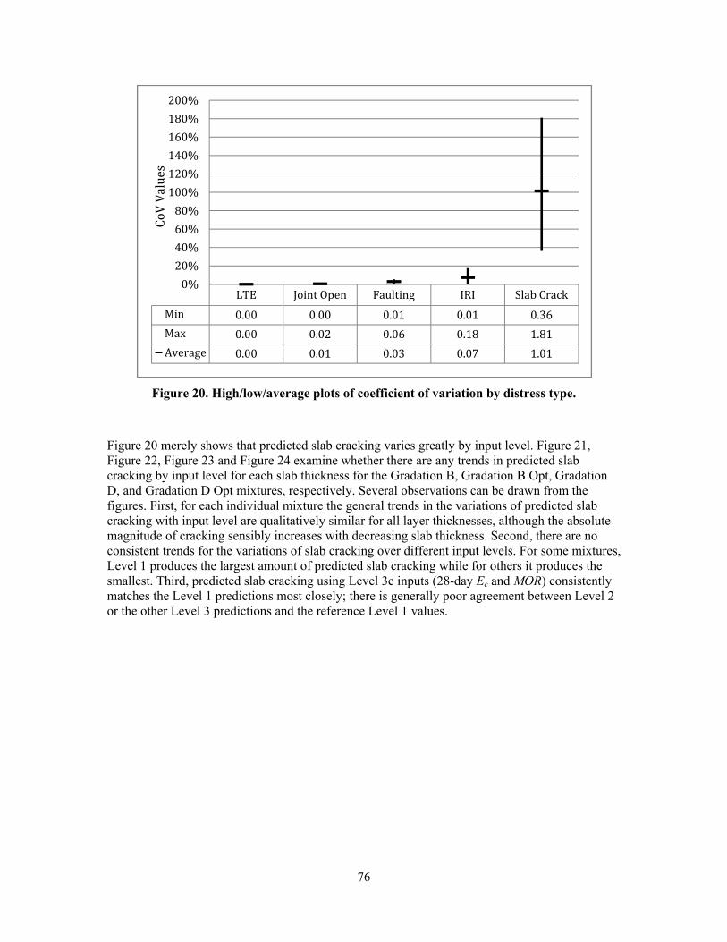
76

Figure 20. High/low/average plots of coefficient of variation by distress type.

Figure 20 merely shows that predicted slab cracking varies greatly by input level. Figure 21, Figure 22, Figure 23 and Figure 24 examine whether there are any trends in predicted slab cracking by input level for each slab thickness for the Gradation B, Gradation B Opt, Gradation D, and Gradation D Opt mixtures, respectively. Several observations can be drawn from the figures. First, for each individual mixture the general trends in the variations of predicted slab cracking with input level are qualitatively similar for all layer thicknesses, although the absolute magnitude of cracking sensibly increases with decreasing slab thickness. Second, there are no consistent trends for the variations of slab cracking over different input levels. For some mixtures, Level 1 produces the largest amount of predicted slab cracking while for others it produces the smallest. Third, predicted slab cracking using Level 3c inputs (28-day Ec and MOR) consistently matches the Level 1 predictions most closely; there is generally poor agreement between Level 2 or the other Level 3 predictions and the reference Level 1 values.

LTE Joint Open Faulting IRI Slab CrackMin 0.00 0.00 0.01 0.01 0.36Max 0.00 0.02 0.06 0.18 1.81Average 0.00 0.01 0.03 0.07 1.01

0%20%40%60%80%100%120%140%160%180%200%

CoVValues

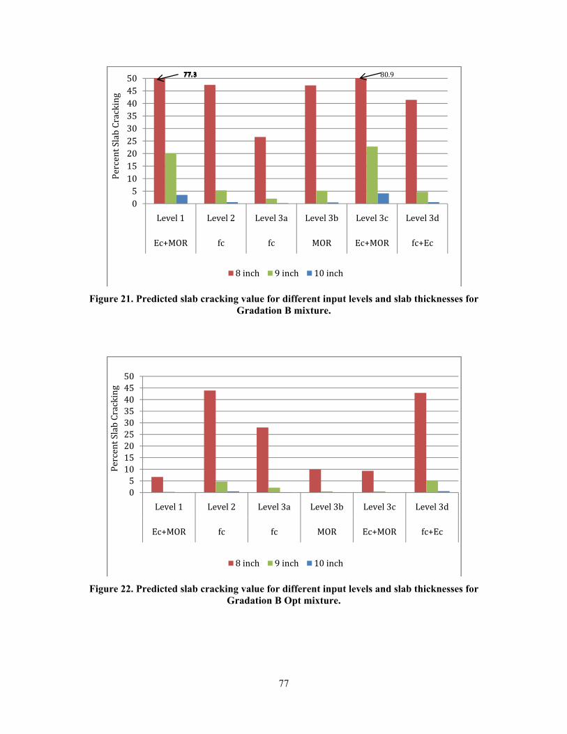
Figu

Figu

ure 21. Predi

ure 22. Predi

05101520253035404550

L

E

Percent Slab Cracking

05101520253035404550

L

Ec

Percent Slab Cracking

icted slab cra

icted slab cra

Level 1 L

c+MOR

Level 1 L

c+MOR

acking value Gradat

acking value Gradatio

evel 2 Lev

fc

8 inch

evel 2 Le

fc

8 inch

77

for differenttion B mixtu

for differenton B Opt mix

vel 3a Lev

fc M

9 inch 1

evel 3a Le

fc M

9 inch 1

t input levelsure.

t input levelsxture.

vel 3b Leve

MOR Ec+M

10 inch

evel 3b Le

MOR Ec

10 inch

s and slab thi

s and slab thi

el 3c Leve

MOR fc+E

80.9

evel 3c Le

c+MOR f

icknesses for

icknesses for

l 3d

Ec

evel 3d

fc+Ec

r

r

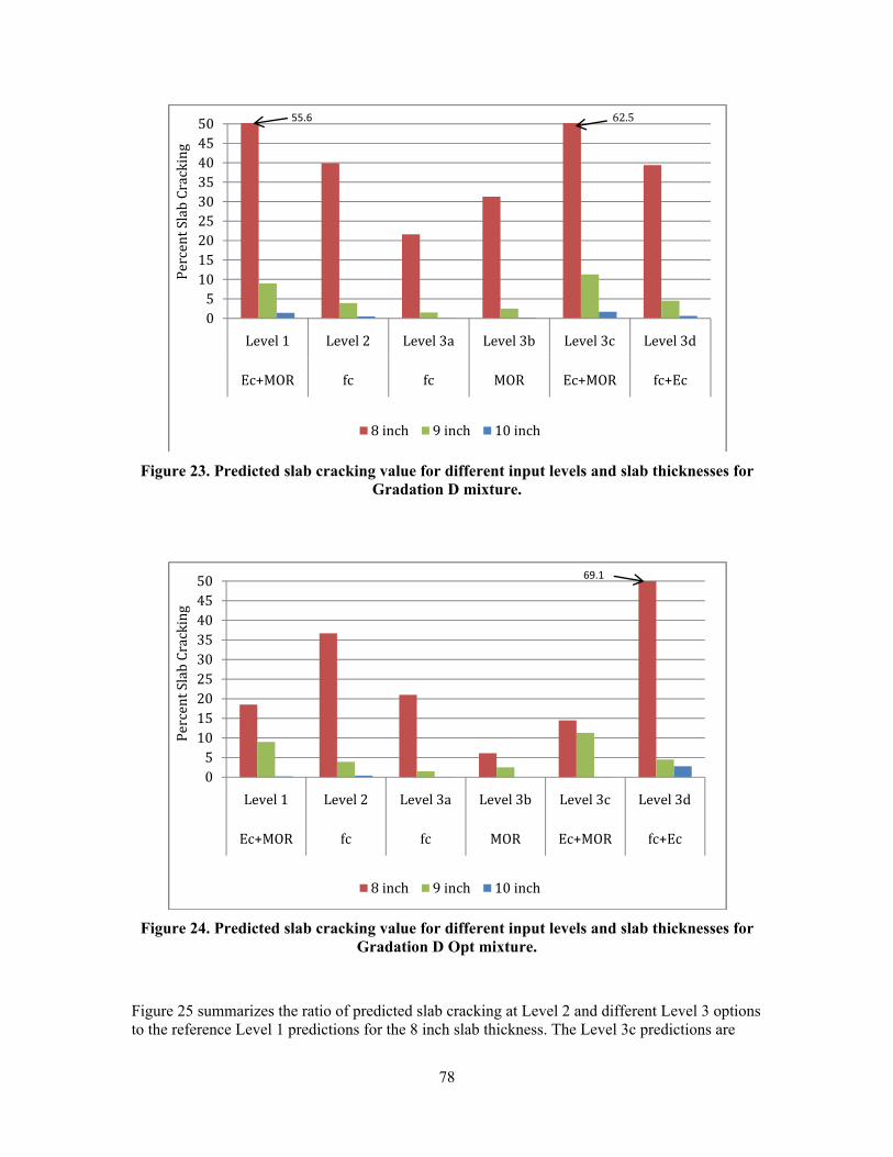
78

Figure 23. Predicted slab cracking value for different input levels and slab thicknesses for

Gradation D mixture.

Figure 24. Predicted slab cracking value for different input levels and slab thicknesses for

Gradation D Opt mixture.

Figure 25 summarizes the ratio of predicted slab cracking at Level 2 and different Level 3 options to the reference Level 1 predictions for the 8 inch slab thickness. The Level 3c predictions are

05101520253035404550

Level 1 Level 2 Level 3a Level 3b Level 3c Level 3d

Ec+MOR fc fc MOR Ec+MOR fc+Ec

Percent Slab Cracking

8 inch 9 inch 10 inch

55.6 62.5

05101520253035404550

Level 1 Level 2 Level 3a Level 3b Level 3c Level 3d

Ec+MOR fc fc MOR Ec+MOR fc+Ec

Percent Slab Cracking

8 inch 9 inch 10 inch

69.1

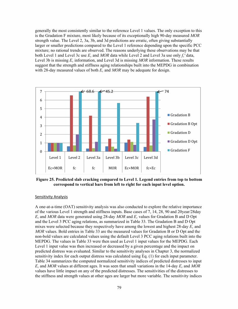
79

generally the most consistently similar to the reference Level 1 values. The only exception to this is the Gradation F mixture, most likely because of its exceptionally high 90-day measured MOR strength value. The Level 2, 3a, 3b, and 3d predictions are erratic, often giving substantially larger or smaller predictions compared to the Level 1 reference depending upon the specific PCC mixture; no rational trends are observed. The reasons underlying these observations may be that both Level 1 and Level 3c use Ec and MOR data while Level 2 and Level 3a use only fc′ data, Level 3b is missing Ec information, and Level 3d is missing MOR information. These results suggest that the strength and stiffness aging relationships built into the MEPDG in combination with 28-day measured values of both Ec and MOR may be adequate for design.

Figure 25. Predicted slab cracking compared to Level 1. Legend entries from top to bottom

correspond to vertical bars from left to right for each input level option.

Sensitivity Analysis  A one-at-a-time (OAT) sensitivity analysis was also conducted to explore the relative importance of the various Level 1 strength and stiffness inputs. Base cases of 7, 14, 28, 90 and 20year/28day Ec and MOR data were generated using 28-day MOR and Ec values for Gradation B and D Opt and the Level 3 PCC aging relations, as summarized in Table 33. The Gradation B and D Opt mixes were selected because they respectively have among the lowest and highest 28-day Ec and MOR values. Bold entries in Table 33 are the measured values for Gradation B or D Opt and the non-bold values are calculated values using the default Level 3 PCC aging relations built into the MEPDG. The values in Table 33 were then used as Level 1 input values for the MEPDG. Each Level 1 input value was then increased or decreased by a given percentage and the impact on predicted distress was evaluated. Similar to the sensitivity analyses in Chapter 3, the normalized sensitivity index for each output distress was calculated using Eq. (1) for each input parameter. Table 34 summarizes the computed normalized sensitivity indices of predicted distresses to input Ec and MOR values at different ages. It was seen that small variations in the 14-day Ec and MOR values have little impact on any of the predicted distresses. The sensitivities of the distresses to the stiffness and strength values at other ages are larger but more variable. The sensitivity indices

0

1

2

3

4

5

6

7

Level 1 Level 2 Level 3a Level 3b Level 3c Level 3d

Ec+MOR fc fc MOR Ec+MOR fc+Ec

Gradation B

Gradation B Opt

Gradation D

Gradation D Opt

Gradation F

68.6 45.2 74

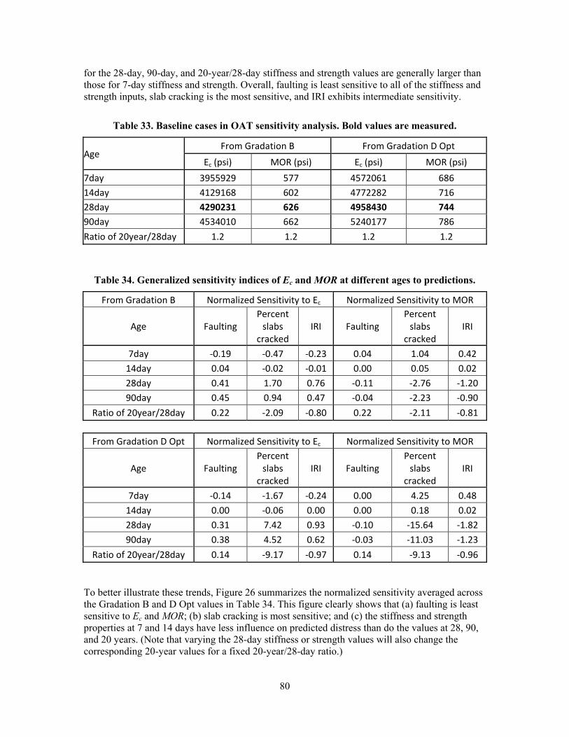
80

for the 28-day, 90-day, and 20-year/28-day stiffness and strength values are generally larger than those for 7-day stiffness and strength. Overall, faulting is least sensitive to all of the stiffness and strength inputs, slab cracking is the most sensitive, and IRI exhibits intermediate sensitivity.

Table 33. Baseline cases in OAT sensitivity analysis. Bold values are measured.

Age From Gradation B  From Gradation D Opt 

Ec (psi)  MOR (psi)  Ec (psi)  MOR (psi) 

7day  3955929  577  4572061  686 14day  4129168  602  4772282  716 28day  4290231  626  4958430  744 90day  4534010  662  5240177  786 

Ratio of 20year/28day  1.2  1.2  1.2  1.2 

Table 34. Generalized sensitivity indices of Ec and MOR at different ages to predictions.

From Gradation B  Normalized Sensitivity to Ec  Normalized Sensitivity to MOR 

Age  Faulting Percent slabs 

cracked IRI  Faulting 

Percent slabs 

cracked IRI 

7day  ‐0.19  ‐0.47  ‐0.23  0.04  1.04  0.42 14day  0.04  ‐0.02  ‐0.01  0.00  0.05  0.02 

28day  0.41  1.70  0.76  ‐0.11  ‐2.76  ‐1.20 90day  0.45  0.94  0.47  ‐0.04  ‐2.23  ‐0.90 

Ratio of 20year/28day  0.22  ‐2.09  ‐0.80  0.22  ‐2.11  ‐0.81  From Gradation D Opt  Normalized Sensitivity to Ec  Normalized Sensitivity to MOR 

Age  Faulting Percent slabs 

cracked IRI  Faulting 

Percent slabs 

cracked IRI 

7day  ‐0.14  ‐1.67  ‐0.24  0.00  4.25  0.48 

14day  0.00  ‐0.06  0.00  0.00  0.18  0.02 28day  0.31  7.42  0.93  ‐0.10  ‐15.64  ‐1.82 

90day  0.38  4.52  0.62  ‐0.03  ‐11.03  ‐1.23 

Ratio of 20year/28day  0.14  ‐9.17  ‐0.97  0.14  ‐9.13  ‐0.96  To better illustrate these trends, Figure 26 summarizes the normalized sensitivity averaged across the Gradation B and D Opt values in Table 34. This figure clearly shows that (a) faulting is least sensitive to Ec and MOR; (b) slab cracking is most sensitive; and (c) the stiffness and strength properties at 7 and 14 days have less influence on predicted distress than do the values at 28, 90, and 20 years. (Note that varying the 28-day stiffness or strength values will also change the corresponding 20-year values for a fixed 20-year/28-day ratio.)

81

Figure 26. Normalized sensitivity of predicted distresses to Ec and MOR values at different

ages.

Summary and Recommendations  The key findings from the analyses reported in this section are as follows:

1. Predicted slab cracking for JPCP is highly sensitive to the input level for Ec and MOR. IRI is also sensitive to input level, primarily because it is a function a slab cracking. Predicted joint faulting and load transfer efficiency are essentially the same at all input levels.

2. Performance predictions using Level 3 inputs of 28-day Ec and MOR closely agree with those using the full Level 1 inputs. Therefore, this Level 3 input combination should be

‐8.00

‐6.00

‐4.00

‐2.00

0.00

2.00

4.00

6.00

Normalized Sensitivity Index

Sensitivity to Ec

Faulting

PercentslabscrackedIRI

‐10.00

‐8.00

‐6.00

‐4.00

‐2.00

0.00

2.00

4.00

Normalized Sensitivity Index

Sensitivity to MOR

Faulting

Percentslabscracked

IRI

82

suitable for most SHA designs.

3. For full Level 1 inputs, predicted performance is most sensitive to 28-day, 90-day, and 20year/28day Ec and MOR inputs and less sensitive to 7-day and 14-day values.

4.3.2 Thermal Properties Previous reviews of the literature (Schwartz and Ceylan, 2010) have documented that rigid pavement performance is very sensitive to surface shortwave absorptivity and the coefficient of thermal expansion, moderately sensitive to thermal conductivity, and insensitive to heat capacity. As described in Table 23, there is no accepted method for measuring surface shortwave absorptivity, so the Level 3 guidelines should be followed for this input. Thermal conductivity can be measured in the laboratory, but as indicated in Table 23 this property is relatively fixed for PCC and therefore the Level 3 default value should suffice for most designs. The strong influence of the coefficient of thermal expansion (CTE) on JPCP performance has been demonstrated in several prior studies (Tanesi et al., 2007; Buch et al., 2008; Kampmann, 2008; Oh and Fernando, 2008; Haider et al., 2008, 2009; Velasquez et al., 2009). Results from these studies suggest that this influence may be inconsistent across different climates. Therefore, a limited sensitivity analysis of predicted pavement performance to CTE for typical Maryland conditions was conducted. The baseline inputs for this sensitivity study are the same as for 8 inch thick Gradation D Opt PCC calculation (the results are shown in first subtable in Table 33). Climate conditions correspond to the Baltimore metropolitan area. A CTE value of 5.5x106/oF was taken as a baseline, and this value was then adjusted +0.1x106/oF to evaluate the sensitivity of predicted distress to CTE. The sensitivity of pavement performance to CTE input is defined in terms of a normalized sensitivity index S:

D CTESCTE DΔ

=Δ (4)

in which ΔD is the change in distress caused by ΔCTE and D and CTE are the corresponding values for the baseline conditions. The results from the CTE sensitivity study are summarized in Figure 27. Faulting and IRI were found to have a high sensitivity to CTE, with sensitivity indices averaging 2.9 and 1.6, respectively. Slab cracking was found to be extremely sensitive to CTE, reaching normalized sensitivity index values of up to 7.3; this means that a 10% increase in CTE will cause a 73% increase in the predicted percentage of cracked slabs. These findings confirm the literature findings that CTE is a critical input for PCC performance predictions in the MEPDG. Consequently, accurate values of CTE will be required for design. Because CTE is important but difficult to measure, a literature review was conducted in an attempt to find good predictive models for estimating CTE. No suitable model was found in this search. The weighted average method incorporated in the MEPDG appears to be the best model currently available. As an added complication, a recent position paper issued by the FHWA (2009) cautions that the current AASHTO TP60 test protocol overestimates CTE by about 15%. Based on the limited

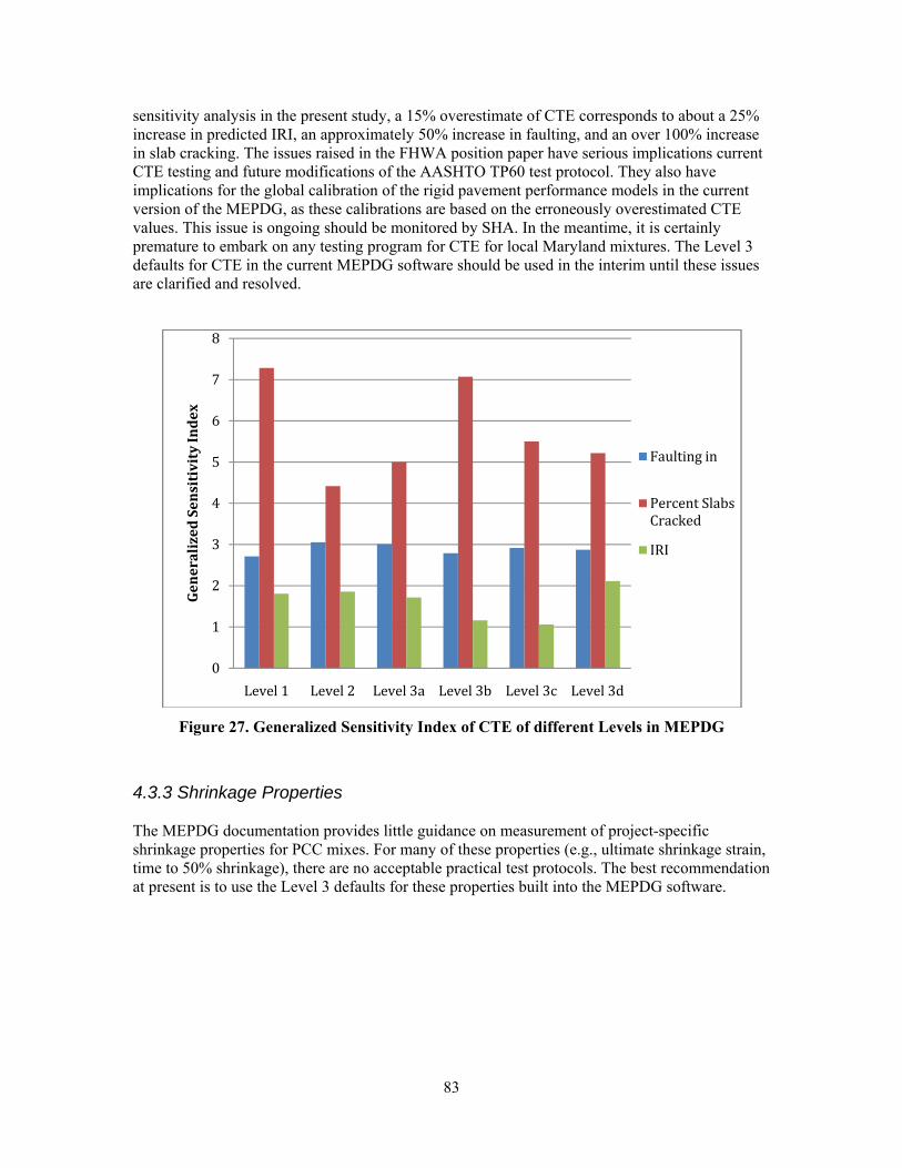
83

sensitivity analysis in the present study, a 15% overestimate of CTE corresponds to about a 25% increase in predicted IRI, an approximately 50% increase in faulting, and an over 100% increase in slab cracking. The issues raised in the FHWA position paper have serious implications current CTE testing and future modifications of the AASHTO TP60 test protocol. They also have implications for the global calibration of the rigid pavement performance models in the current version of the MEPDG, as these calibrations are based on the erroneously overestimated CTE values. This issue is ongoing should be monitored by SHA. In the meantime, it is certainly premature to embark on any testing program for CTE for local Maryland mixtures. The Level 3 defaults for CTE in the current MEPDG software should be used in the interim until these issues are clarified and resolved.

Figure 27. Generalized Sensitivity Index of CTE of different Levels in MEPDG

4.3.3 Shrinkage Properties The MEPDG documentation provides little guidance on measurement of project-specific shrinkage properties for PCC mixes. For many of these properties (e.g., ultimate shrinkage strain, time to 50% shrinkage), there are no acceptable practical test protocols. The best recommendation at present is to use the Level 3 defaults for these properties built into the MEPDG software.

0

1

2

3

4

5

6

7

8

Level 1 Level 2 Level 3a Level 3b Level 3c Level 3d

Generalized Sensitivity Index

Faulting in

Percent Slabs Cracked

IRI

84

4.4 Summary

4.4.1 Testing Recommendations There is very little data on the physical and mechanical properties Maryland PCC mixes to be incorporated into the database at this time. Much of the physical data required by the MEPDG (e.g., cement type, cementitious material content, water/cement ratio) is routinely available for individual projects and should be collected and entered into the database. Continued measurement of split cylinder tensile strength should be discontinued, as this is not a primary input to the MEPDG (or to the 93 AASHTO Design Guide). Instead, 28-day PCC elastic modulus and modulus of rupture should be measured for JPCP paving projects in the future, incorporated into the database, and used for Level 3 inputs to the MEPDG. There is no documented need to perform additional laboratory testing to determine the full Level 1 stiffness and strength inputs for PCC. Given the lack of practical accepted test standards, ongoing test protocol issues, and other reasons, it is recommended that SHA not embark on any additional testing for thermal or shrinkage properties at this time. The current version of the MEPDG has been calibrated using the default Level 3 values for these properties, and these default values should continue to be used until accepted testing standards are available. 4.4.2 Recommended MEPDG Inputs The recommended PCC inputs for the MEPDG are summarized in Table 35 through Table 38 below.

Table 35. Recommended PCC thermal and shrinkage property inputs for Maryland conditions (all JPCP construction types).

Property Input Level

Value Comment

General Properties PCC Material 3 JPCP Only option available. Layer thickness 1 Project specific Unit weight 3 150 pcf MEPDG default Poisson’s ratio 3 0.2 MEPDG default Thermal Properties Coefficient of thermal expansion

3 5.5x10-2/oF MEPDG default (global calibration value).

Thermal conductivity 3 1.25 BTU/hr-ft-oF MEPDG default (global calibration value). Heat capacity 3 0.28 BTU/lb-ft MEPDG default (global calibration value).

85

Table 36. Recommended PCC mix property inputs for Maryland conditions.

Property Input Level

Value Comment

Cement type 1 Type 1 Based on Mix 7 data from Salisbury bypass; should be replaced by mix-specific value if available

Cementitious material content

1 580 lb/cy Based on Mix 7 data from Salisbury bypass; should be replaced by mix-specific value if available

Water/cement ratio 1 0.44 Based on Mix 7 data from Salisbury bypass; should be replaced by mix-specific value if available

Aggregate type 1 Limestone Based on Mix 7 data from Salisbury bypass; should be replaced by mix-specific value if available

PCC zero stress temperature

3 Project specific Default calculated by MEDPG as function of site weather conditions and cementitious material content

Ultimate shrinkage 2 Project specific Default calculated by MEPDG as function of cement type, cement content, water/cement ratio, 28-day compressive strength, and curing conditions

Reversible shrinkage 3 50% Value used in global calibration of distress models Time to develop 50% shrinkage

3 35 days Value used in global calibration of distress models

Curing method 1 Project specific

Table 37. Recommended strength and stiffness input properties for new PCC for Maryland conditions (new/reconstruction/rehabilitation designs).

Property Input Level

Value Comment

28-day PCC modulus of rupture

3 685 psi Based on Mix 7 split cylinder tensile strength from Salisbury bypass and empirical conversion; should be replaced by mix-specific value if available

28-day PCC elastic modulus

3 4,371,000 psi Based on Mix 7 split cylinder tensile strength from Salisbury bypass and empirical conversion; should be replaced by mix-specific value if available

Table 38. Recommended strength and stiffness input properties for existing PCC for Maryland conditions (rehabilitation designs).

Property Input Level

Value Comment

28-day PCC compressive strength

2 Project specific Obtained from cores of existing PCC slab.

87

5. UNBOUND MATERIAL DATA 5.1 MEPDG Input Requirements The principal mechanical property for unbound materials is the resilient modulus at the reference condition of optimum moisture and in-place density (AASHTO T180). The input requirements for resilient modulus vary by input level:

• Level 1

o Laboratory Measurement (New Construction/Reconstruction): The regression coefficients k1, k2, and k3 for the stress-dependent resilient modulus relationship (AASHTO T307 or NCHRP 1-28A):

2 3

1 1k k

octR a

a a

M k pp p

τθ⎛ ⎞ ⎛ ⎞= +⎜ ⎟ ⎜ ⎟

⎝ ⎠ ⎝ ⎠ (5)

in which:

MR = resilient modulus θ = bulk stress = σ1 + σ2 + σ3

τoct = octahedral shear stress = ( ) ( ) ( )2 2 2

1 2 2 3 1 3

13

σ σ σ σ σ σ− + − + −

σ1,σ2,σ3 = principal stresses pa = atmospheric pressure (normalizing factor)

o Field Measurement (Rehabilitation/Overlay Design): FWD backcalculated EFWD values (AASHTO T256/ASTM D5858). These field backcalculated EFWD value must be converted to an equivalent laboratory MR value using the adjustment factors in Table 39.

• Level 2 - MR determined from correlations with California Bearing Ratio, R-value, structural layer coefficient ai, or plasticity index and gradation as summarized in Table 40.

• Level 3 - Default MR at optimum moisture and density as a function of AASHTO soil type as summarized in Table 41.

In addition to stiffness, hydraulic properties for the partially saturated unbound materials in the base, subbase, and subgrade layers are required as inputs for the Enhanced Integrated Climate Model (EICM) built into the MEPDG.3 The principal hydraulic properties for unbound materials are the saturated hydraulic conductivity (permeability) and the soil water characteristic curve (SWCC). The input requirements for these vary by input level:

• Level 1 – Measured saturated hydraulic conductivity (AASHTO T215) and measured soil water characteristic curve (ASTM D6836) for determining parameters of the Fredlund-

3 Note that the details of the relations for the EICM inputs in the current version of the MEPDG have changed slightly from the descriptions in the NCHPR 1-37A final report. The updated formulation is described in Zapata and Houston (2008) and in Zapata et al. (2009).

88

Xing (1994) model.

• Level 2/3 – Default saturated hydraulic conductivity as a function of gradation and plasticity index; default Fredlund-Xing SWCC parameters as f unction of gradation (nonplastic/coarse soils) or gradation and plasticity (plastic/fine-grained soils).

Additional mechanical and physical property data required at all input levels in the MEPDG include:

• Gradation (AASHTO T88) • Atterberg limits (AASHTO T89, T90) • Specific gravity of solids Gs (AASHTO T100) • Maximum dry density and optimum moisture content (AASHTO T180) • Poisson’s ratio ν • Coefficient of lateral earth pressure K0

Default values for these properties for each AASHTO soil class are provided in the MEPDG software. These default values can be replaced by project-specific data if available.

Table 39. Ratio of laboratory MR to field backcalculated EFWD modulus values for unbound materials (AASHTO, 2008).

Layer Type Location MR/EFWD

Aggregate Base/Subbase Between a stabilized and HMA layer 1.43 Below a PCC layer 1.32 Below an HMA layer 0.62

Subgrade/Embankment Below a stabilized subgrade/embankment 0.75 Below an HMA or PCC layer 0.52 Below an unbound aggregate base 0.35

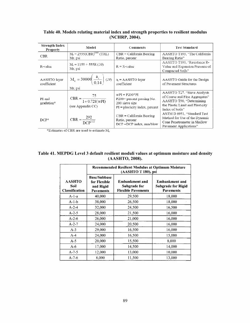
89

Table 40. Models relating material index and strength properties to resilient modulus (NCHRP, 2004).

Table 41. MEPDG Level 3 default resilient moduli values at optimum moisture and density (AASHTO, 2008).

90

5.2 Summary of Data and Preliminary Analysis A total of 85 acceptable sets of unbound properties were provided by SHA for initial population of the material properties database. Each set of data contained the following unbound material properties: AASHTO class and Group Index; Atterberg limits (PI and LL); percents passing the No. 4 and No. 200 sieves; moisture content, saturation, and dry density at optimum conditions (AASHTO T180 assumed) and at other resilient modulus testing conditions; one or more sets of laboratory-measured resilient modulus data. Considerable effort was devoted to identify incorrect or inconsistent information in the data provided by SHA. Incorrect or inconsistent data were corrected when possible and eliminated when not. The key mechanical property required for unbound base/subbase/subgrade materials is the resilient modulus, MR, at optimum moisture content and in-place density. For Level 1 inputs, the stress dependence of MR must also be included as determined from the AASHTO T307, LTPP P46, or NCHRP 1-28A test protocols. The scope of the provided data is described in Table 42. Many of the soils had laboratory measured MR data at multiple moisture contents (typically optimum and optimum+2%).There are multiple MR testing records for each moisture condition since MR is measured at different stress states. Gradation information was limited to the percents passing the No. 4 and No. 200 sieves. Other properties received included the PI, LL, maximum dry unit weight, optimum gravity water content, saturation degree at optimum condition were also received. No hydraulic properties (e.g., hydraulic conductivity) were provided.

Table 42. Number of test records received from SHA.

Classification Number of Property

Sets

Number of Acceptable MR

Records

A-1-b 3 44 A-2-4 17 575 A-2-6 6 103 A-3 1 56 A-4 33 1331 A-5 1 42 A-6 13 463 A-7-5 4 168 A-7-6 2 84 Classification Not Mentioned 5 45

TOTAL 85 2911 The mean and ranges of values for the unbound material supplied by SHA are summarized in Figure 28 through Figure 31. These summaries include MR at 95% compaction and optimum moisture content (Figure 28), optimum moisture content (Figure 29), degree of saturation at

91

optimum moisture (Figure 30), and maximum dry unit weight (Figure 31) for each soil type. The grey bars (right axis) indicate the number of test records included in the database, the heavy black vertical lines (left axis) indicate the ranges of the data, and the heavy black short horizontal lines indicate the mean values. Noteworthy observations regarding the data in these figures include the following:

• The A-2-4, A-4 and A-6 are the most common unbound material in the data set. There is not much data for the A-1-b, A-2-6, A-3, A-5, A-7-5, and A-7-6 soil classes.

• The ranges of the MR value are large for all soil types. This is because all stress states are included in the chart.

• The ranges of optimum moisture content, saturation at optimum, and maximum dry unit weight are within reasonable limits.

Figure 28. Averages and ranges of resilient modulus values at 95% compaction and

optimum moisture content (includes all stress states).

92

Figure 29. Averages and ranges of optimum water contents.

Figure 30. Averages and ranges of saturation levels at optimum moisture.

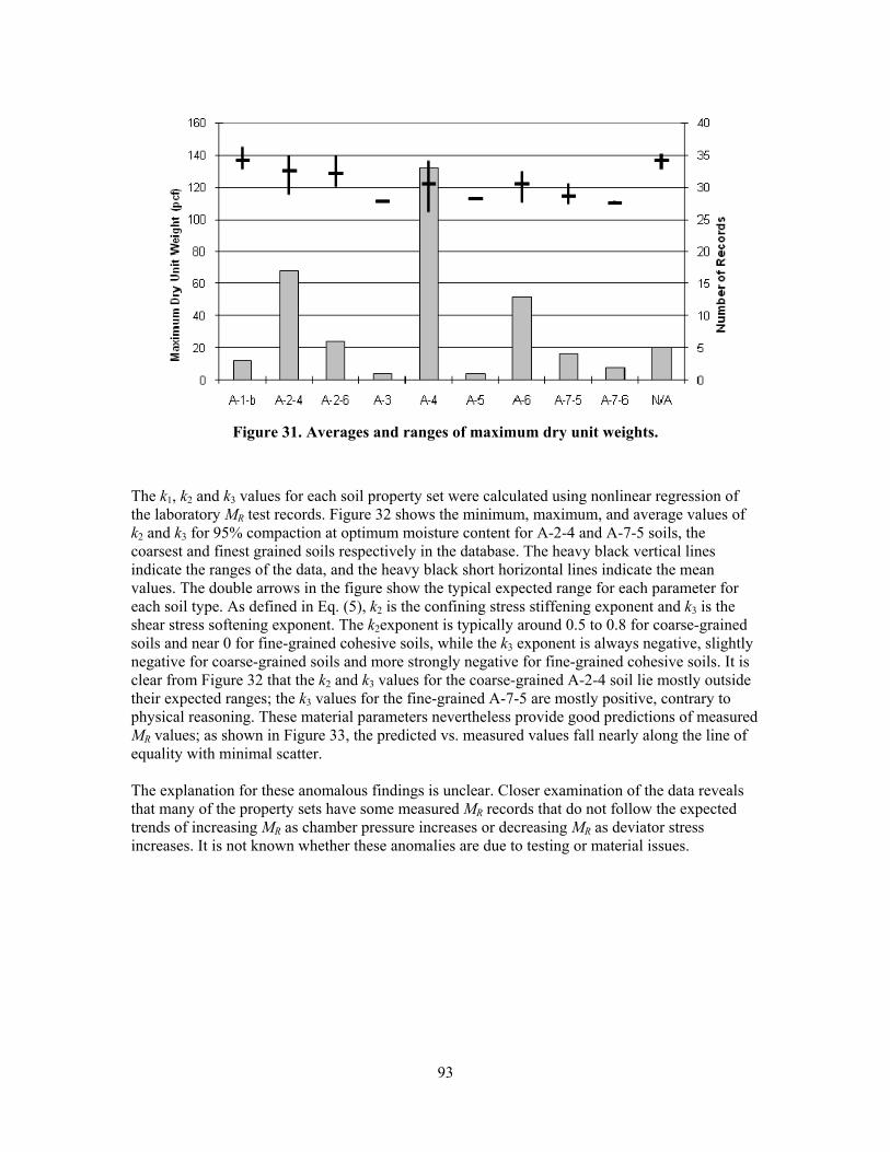
93

Figure 31. Averages and ranges of maximum dry unit weights.

The k1, k2 and k3 values for each soil property set were calculated using nonlinear regression of the laboratory MR test records. Figure 32 shows the minimum, maximum, and average values of k2 and k3 for 95% compaction at optimum moisture content for A-2-4 and A-7-5 soils, the coarsest and finest grained soils respectively in the database. The heavy black vertical lines indicate the ranges of the data, and the heavy black short horizontal lines indicate the mean values. The double arrows in the figure show the typical expected range for each parameter for each soil type. As defined in Eq. (5), k2 is the confining stress stiffening exponent and k3 is the shear stress softening exponent. The k2exponent is typically around 0.5 to 0.8 for coarse-grained soils and near 0 for fine-grained cohesive soils, while the k3 exponent is always negative, slightly negative for coarse-grained soils and more strongly negative for fine-grained cohesive soils. It is clear from Figure 32 that the k2 and k3 values for the coarse-grained A-2-4 soil lie mostly outside their expected ranges; the k3 values for the fine-grained A-7-5 are mostly positive, contrary to physical reasoning. These material parameters nevertheless provide good predictions of measured MR values; as shown in Figure 33, the predicted vs. measured values fall nearly along the line of equality with minimal scatter. The explanation for these anomalous findings is unclear. Closer examination of the data reveals that many of the property sets have some measured MR records that do not follow the expected trends of increasing MR as chamber pressure increases or decreasing MR as deviator stress increases. It is not known whether these anomalies are due to testing or material issues.

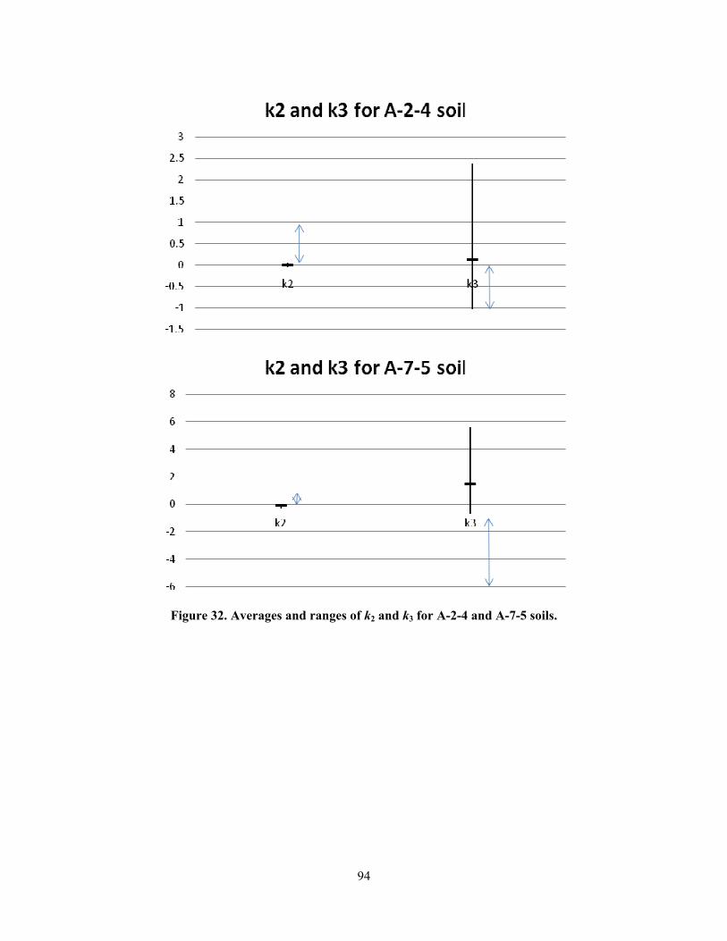
94

Figure 32. Averages and ranges of k2 and k3 for A-2-4 and A-7-5 soils.

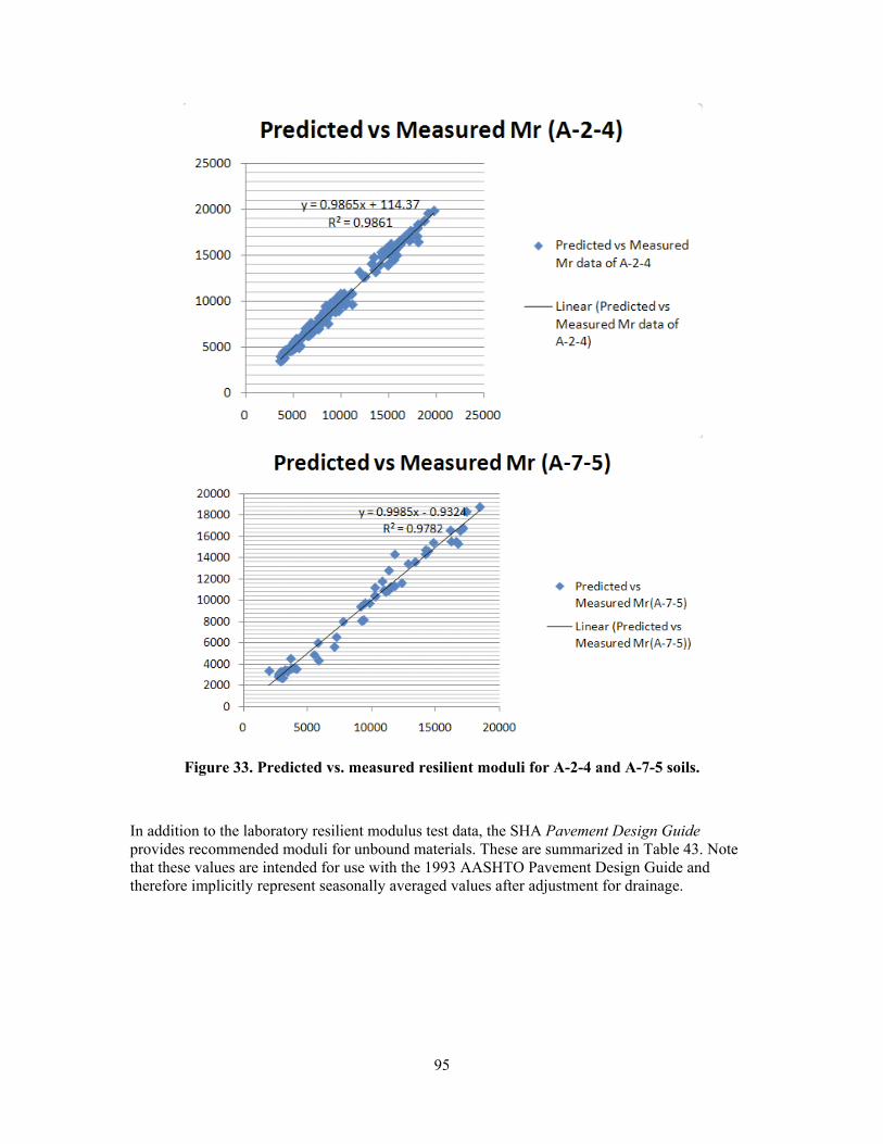
95

Figure 33. Predicted vs. measured resilient moduli for A-2-4 and A-7-5 soils.

In addition to the laboratory resilient modulus test data, the SHA Pavement Design Guide provides recommended moduli for unbound materials. These are summarized in Table 43. Note that these values are intended for use with the 1993 AASHTO Pavement Design Guide and therefore implicitly represent seasonally averaged values after adjustment for drainage.

96

Table 43. Recommended moduli for unbound materials from SHA Pavement Design Guide.

Material Modulus (psi) Minimum Typical Maximum

Base/Subbase Materials Graded Aggregate Base 15,000 25,000 45,000 Gravel 10,000 15,000 30,000 Soil Contaminated Aggregate Base 3,000 10,000 20,000 Capping Borrow 10,500 10,500 10,500 Subgrade Soils Silts and Clays (w/ high compressibility) 1,000 – 2000 Fine Grained Soils with Silts and Clays (w/ low compressibility)

2,000 – 3,000

Poorly Graded Sands 3,000 – 4,500 Gravely Soils, Well Graded Sands, and Sand/Gravel Mixtures

4,500 – 10,000

5.3 Analyses of Unbound Material Properties 5.3.1 Stiffness Properties Input Level  Level 1 unbound resilient modulus inputs are not recommended for use in the MEPDG at this time for the following reasons:

1. Input of Level 1 properties for unbound materials automatically switches the MEPDG structural analysis model from multilayer elastic theory to finite element analysis. The execution time for the flexible pavement finite element calculations in the current version of the MEPDG is far too long for practical usage.

2. Performance predictions using Level 1 unbound material properties have not been calibrated in the current version of the MEPDG.

Both of these issues will likely change in future versions of the MEPDG. However, to date there have been no published studies using Level 1 unbound material inputs to provide any guidance on the sensitivity of predicted performance to resilient modulus input level. Unlike many agencies, the Maryland SHA is well-equipped to perform Level 1 laboratory characterization of unbound materials, and the SHA testing effort to date has practical value despite the recommendations against Level 1 unbound resilient modulus inputs in the current version of the MEPDG. Laboratory measurements can be evaluated for expected in-service stress states to develop improved estimates of MR values for Level 2/3 input. However, this requires estimates of typical in situ stress states for granular base layers and subgrades. The 1993 AASHTO Design Guide provides typical values for the bulk stress θ for granular base layers. These are summarized in Table 44. Since the 1993 AASHTO Guide does not consider shear stress effects for granular base layers, no typical values for the octahedral shear stress τoct

97

are provided. For typical Maryland pavement conditions, the data in Table 44 suggest a bulk stress θ in the range of 5 to 10 psi for granular base layers.

Table 44. Suggested bulk stress θ (psi) values for use in design of granular base layers (AASHTO, 1993).

Asphalt Concrete Thickness (inches*)

Subgrade Resilient Modulus (psi*) 3,000 7,500 15,000

< 2 20 25 30 2 – 4 10 15 20 4 – 6 5 10 15 > 6 5 5 5

*1 inch = 25.4 mm; 1 psi = 6.9 kPa Von Quintus and Killingsworth (1997a, 1997b) provide examples for estimating the stress state in granular base and subgrade for an individual pavement structure. The representative conditions are taken at one-quarter depth into the granular base layer and 18 inches below the top of subgrade for a 9 kip wheel load. In situ stresses at these locations based on the material unit weights and the coefficients of lateral stress are combined with the load-induced stresses computed using multilayer elastic theory and reasonable preliminary estimates of the layer moduli. Seasonal effects due to moisture variations can also be included in the calculations. Table 45 summarizes for typical Maryland conditions the stress states in the granular base and subgrade layers computed using Von Quintus and Killingsworth’s approach. The HMA stiffness was assumed as 250,000 psi in all cases and the base layer stiffness was estimated as 25,000 psi. The load consisted of a 9000 lb tire having a 120 psi pressure. Full-slip conditions were assumed at the layer interface. All stress states also include the influence of the in situ stresses. The average computed stress states over all HMA and granular base thickness and subgrade MR conditions were θ ≅ 40 psi, τoct ≅ 3.5 psi for the granular base layer and θ ≅ 10 psi, τoct ≅ 2 psi for the subgrade.

Table 45. Stress states for various typical Maryland pavement structures.

Richter (Richter, 2002; Richter and Schwartz, 2002) used multilayer elastic theory to estimate stress states at various locations within granular base/subbase layers and subgrades for field sections in the LTPP Seasonal Monitoring Program. These calculations were part of an effort to

z (in) σv (psi) σh (psi) θ (psi) τoct (psi) z (in) σv (psi) σh (psi) θ (psi) τoct (psi)4 8 2000 6 31.005 25.418 82.84 2.75 30 3.858 0.605 10.07 2.12

5000 6 34.031 20.609 76.25 6.45 30 5.308 0.582 11.47 2.8212 2000 7 33.919 19.598 74.28 6.89 34 2.932 0.571 9.74 1.78

5000 7 35.264 15.931 68.29 9.25 34 4.205 0.606 11.08 2.3610 8 2000 12 5.007 4.796 16.60 0.34 36 1.427 0.415 8.26 1.18

5000 12 6.43 4.281 16.99 1.25 36 2.215 0.517 9.25 1.5112 2000 13 6.364 5.142 18.81 0.83 40 1.328 0.403 8.80 1.22

5000 13 7.416 4.408 18.40 1.67 40 2.048 0.508 9.73 1.5116 2000 14 7.163 4.969 19.43 1.31 44 1.196 0.383 9.30 1.25

5000 14 7.914 4.152 18.55 2.05 44 1.843 0.49 10.16 1.50MINIMUM 16.60 0.34 8.26 1.18MAXIMUM 82.84 9.25 11.47 2.82AVERAGE 41.05 3.28 9.79 1.73

Base - Quarter Depth Subgrade - 18 in DepthD1 (in) D2 (in)

Subgrade MR (psi)

98

evaluate stress dependency of backcalculated layer moduli. Her calculated stresses are summarized in Figure 34 for granular base/subbase layers and in Figure 35 and Figure 36 for coarse and fine grained subgrades, respectively. Ranges of stress states encompassing most of the data points in these figures are summarized in Table 46 after conversion to U.S. Customary units.

Figure 34. Calculated stress states for granular base and subbase layers (Richter, 2002).

99

Figure 35. Calculated stress states for coarse grained subgrade soils (Richter, 2002).

Figure 36. Calculated stress states for fine grained subgrade soils (Richter, 2002).

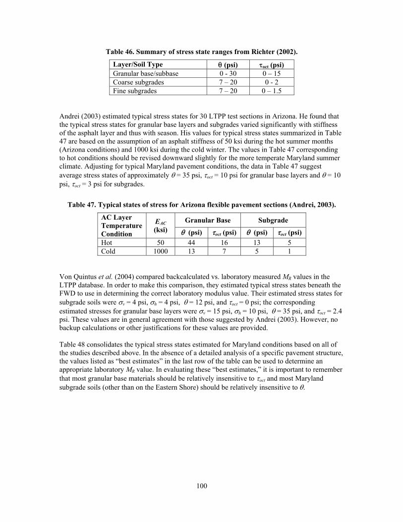
100

Table 46. Summary of stress state ranges from Richter (2002).

Layer/Soil Type θ (psi) τoct (psi) Granular base/subbase 0 - 30 0 – 15 Coarse subgrades 7 – 20 0 - 2 Fine subgrades 7 – 20 0 – 1.5

Andrei (2003) estimated typical stress states for 30 LTPP test sections in Arizona. He found that the typical stress states for granular base layers and subgrades varied significantly with stiffness of the asphalt layer and thus with season. His values for typical stress states summarized in Table 47 are based on the assumption of an asphalt stiffness of 50 ksi during the hot summer months (Arizona conditions) and 1000 ksi during the cold winter. The values in Table 47 corresponding to hot conditions should be revised downward slightly for the more temperate Maryland summer climate. Adjusting for typical Maryland pavement conditions, the data in Table 47 suggest average stress states of approximately θ = 35 psi, τoct = 10 psi for granular base layers and θ = 10 psi, τoct = 3 psi for subgrades.

Table 47. Typical states of stress for Arizona flexible pavement sections (Andrei, 2003).

AC Layer Temperature Condition

EAC (ksi)

Granular Base Subgrade

θ (psi) τoct (psi) θ (psi) τoct (psi) Hot 50 44 16 13 5 Cold 1000 13 7 5 1

Von Quintus et al. (2004) compared backcalculated vs. laboratory measured MR values in the LTPP database. In order to make this comparison, they estimated typical stress states beneath the FWD to use in determining the correct laboratory modulus value. Their estimated stress states for subgrade soils were σv = 4 psi, σh = 4 psi, θ = 12 psi, and τoct = 0 psi; the corresponding estimated stresses for granular base layers were σv = 15 psi, σh = 10 psi, θ = 35 psi, and τoct = 2.4 psi. These values are in general agreement with those suggested by Andrei (2003). However, no backup calculations or other justifications for these values are provided. Table 48 consolidates the typical stress states estimated for Maryland conditions based on all of the studies described above. In the absence of a detailed analysis of a specific pavement structure, the values listed as “best estimates” in the last row of the table can be used to determine an appropriate laboratory MR value. In evaluating these “best estimates,” it is important to remember that most granular base materials should be relatively insensitive to τoct and most Maryland subgrade soils (other than on the Eastern Shore) should be relatively insensitive to θ.

101

Table 48. Consolidated estimates of pavement stress states for Maryland conditions.

Source Granular Base Subgrade

θ (psi) τoct (psi) θ (psi) τoct (psi) 1993 AASHTO 5 – 10 Von Quintus and Killingsworth (1997a, 1997b) – Table 45

40 3.5 10 2

Richter (2002) 0 – 30 0 – 15 7 – 20 0 – 1.5 Andrei (2003) 35 10 10 3 Von Quintus et al. (2004) 35 2.4 12 0 Best Estimate 30 5 12 2

The k1, k2, and k3 resilient modulus parameters for Eq. (5) were evaluated for the laboratory MR measurements provided by SHA and then Eq. (5) was evaluated for the “best estimate” stress states in Table 48. The results from this analysis are summarized in Table 49 by AASHTO soil class and moisture condition. In cases where multiple sets of test records are available, both the mean and the range of values are reported. Some soils are typical only of base conditions (e.g., A-1-b), some could be either base/subbase or subgrade soils (e.g., A-2-4), and some are encountered only in subgrades (e.g., A-7-5). The appropriate MR values at the appropriate stress state are given for each case. The shaded entries in the table indicate values that appear to be excessively high or low for the given soil class and moisture condition. Note that the measured MR values in Table 48 for subbase materials (A-2-4, A-2-6) are slightly lower on average but within the range of values in Table 43 that SHA currently uses in its 1993 AASHTO designs (e.g., soil contaminated granular base). Conversely, the measured MR values in Table 48 for fine-grained subgrade materials (A-4, A-6) are higher than those in Table 43. However, the values in Table 43 are intended for use in the 1993 AASHTO Pavement Design Guide and implicitly include seasonal effects and drainage influences.

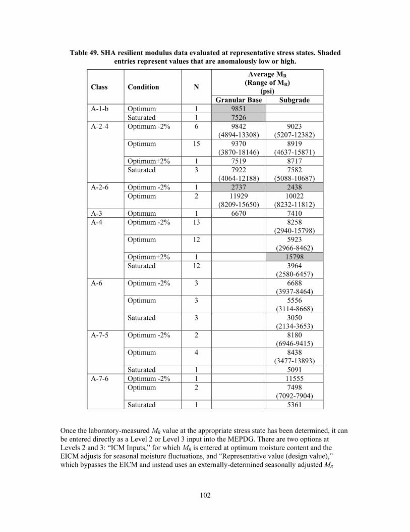
102

Table 49. SHA resilient modulus data evaluated at representative stress states. Shaded entries represent values that are anomalously low or high.

Class Condition N

Average MR (Range of MR)

(psi) Granular Base Subgrade

A-1-b Optimum 1 9851 Saturated 1 7526

A-2-4 Optimum -2% 6 9842 (4894-13308)

9023 (5207-12382)

Optimum 15 9370 (3870-18146)

8919 (4637-15871)

Optimum+2% 1 7519 8717 Saturated 3 7922

(4064-12188) 7582

(5088-10687) A-2-6 Optimum -2% 1 2737 2438

Optimum 2 11929 (8209-15650)

10022 (8232-11812)

A-3 Optimum 1 6670 7410 A-4 Optimum -2% 13

8258

(2940-15798) Optimum 12

5923

(2966-8462) Optimum+2% 1 15798 Saturated 12

3964

(2580-6457) A-6 Optimum -2% 3

6688

(3937-8464) Optimum 3

5556

(3114-8668) Saturated 3

3050

(2134-3653) A-7-5 Optimum -2% 2

8180

(6946-9415) Optimum 4

8438

(3477-13893) Saturated 1 5091

A-7-6 Optimum -2% 1 11555 Optimum 2

7498

(7092-7904) Saturated 1 5361

Once the laboratory-measured MR value at the appropriate stress state has been determined, it can be entered directly as a Level 2 or Level 3 input into the MEPDG. There are two options at Levels 2 and 3: “ICM Inputs,” for which MR is entered at optimum moisture content and the EICM adjusts for seasonal moisture fluctuations, and “Representative value (design value),” which bypasses the EICM and instead uses an externally-determined seasonally adjusted MR

103

(similar in concept to 1993 AASHTO approach). The equation used by the EICM for moisture effects is given as (Andrei, 2003):

( )( )10

,

log1 s opt

Rk S S

R opt

M b aaM e β + −

−= +

+ (6)

in which: MR = resilient modulus at field saturation S MR,opt = resilient modulus at maximum dry density and optimum moisture a = minimum value of the log of the modulus ratio b = maximum value of the log of the modulus ratio β = location parameter = ln(-b/a) ks = regression parameter (S-Sopt) = deviation of field saturation from optimum (decimal) Values for the coefficients in Eq. (6) as implemented in the MEPDG are given in Table 50. Equation (6) can also be used for external estimation of a seasonally adjusted MR.

Table 50. MEPDG values of a, b, and ks for Eq. (6).

Parameter Coarse-Grained Materials

Fine-Grained Materials

a -0.3123 -0.5934 b 0.3 0.4 ks 6.8157 6.1324

Yau and Von Quintus (2001) performed an extensive analysis of the LTPP database to determine regressions between k1, k2, and k3 in Eq. (5) as a function of gradation, Atterberg limits, and other physical properties. However, these regressions are more appropriately used when no laboratory resilient modulus test data are available. Sensitivity Analysis  The strong impact of base and subgrade stiffness on pavement performance is well-known from practical experience, from the 1993 AASHTO Design Guide, and from numerous MEPDG sensitivity studies reported in the literature (e.g., Masad and Little, 2004; El-Basyouny and Witczak 2005a, 2005b, 2005c; Carvalho and Schwartz, 2006; Hoerner et al., 2007; Schwartz, 2009; Ayyala et al., 2010). For example, Schwartz (2009) examined predicted service life as a function of granular base and subgrade properties for typical flexible pavement sections using both the 1993 AASHTO and MEPDG procedures. Figure 37 and Figure 38 summarize the sensitivity of predicted service life to base and subgrade stiffness, respectively, for a granular base layer thickness D2 = 12 inches and three HMA layer thicknesses D1 = 3, 6, and 9 inches. Reliability was set at 50% for both the AASHTO and MEPDG procedures. The strong impact of base and subgrade stiffness on predicted service life is clearly evident in all cases. There also is good agreement in the trends of the two design methods for the thin (3 inch) and medium (6 inch) asphalt layer cases. However, for the thick (9 inch) asphalt case, the sensitivity of service life to base modulus for the AASHTO design procedure is much greater than that for the MEPDG, as indicated by the steeper slope in the curve in Figure 38. Moreover, there is a crossing point for the thick asphalt case; the AASHTO procedure predicts much longer service life for pavements with high quality thick bases than does the MEPDG, but the reverse is true for low quality bases in this

104

scenario. These trends and other similar results from the literature emphasize that good estimates of the resilient modulus of the unbound layers are important for accurate pavement performance prediction.

Figure 37. Predicted service life vs. subgrade resilient modulus; base modulus = 30,600 psi

(Schwartz, 2009).

Figure 38. Predicted service life vs. granular base modulus; subgrade modulus = 5000 psi

(Schwartz, 2009).

0

10

20

30

40

50

0 5000 10000 15000Subgrade Mr (psi)

Serv

ice

Life

N18

(x1M

)

AASHTO D1=9MEPDG D1=9AASHTO D1=6MEPDG D1=6AASHTO D1=3MEPDG D1=3

0

10

20

30

40

50

20000 30000 40000 50000Base Modulus (psi)

Serv

ice

Life

N18

(x1M

)

AASHTO D1=9MEPDG D1=9AASHTO D1=6MEPDG D1=6AASHTO D1=3MEPDG D1=3

105

5.3.2 Hydraulic Properties Input Level  The environmental model in the MEPDG is a one-dimensional formulation for vertical heat and partially-saturated moisture flows in the pavement system. Some of the assumptions in the MEPDG analyses include: zero rainfall infiltration through the pavement surface; no lateral flow to edge drains; liquid flow only—i.e., no vapor flow; uncoupled heat and fluid flow; and unbound material thermal conductivity and heat capacity values set internally to typical default values. The principal hydraulic inputs in the MEPDG are the saturated hydraulic conductivity or permeability (ks) and the parameters defining the soil-water characteristic curve (SWCC) for unsaturated soil conditions typical of unbound materials beneath pavements. Saturated hydraulic conductivity (permeability) is a familiar property to most geotechnical and pavement engineers. The SWCC generally is not. The SWCC is a fundamental property of unsaturated soils that soil matric suction (in conceptual terms, the negative porewater pressure in a partially saturated soil) and water content as shown in Figure 39. The SWCC is required for analyses of water movement under partially saturated conditions. It is also used in characterizing the shear strength and compressibility of unsaturated soils, and the unsaturated hydraulic conductivity of soil is often estimated using properties from the SWCC together with the saturated hydraulic conductivity. The issue of Level 1 vs. Level 2 vs. Level 3 inputs for these properties is less significant than for other MEPDG inputs for several reasons:

• Few geotechnical laboratories, including the one at SHA, are equipped with the pressure plate apparatus (ASTM D3152-72) required to determine the level 1 SWCC inputs. In addition, this test procedure is exacting, time-consuming, and expensive to perform.

• The developers of the MEPDG expended considerable energy to develop a simplified yet accurate approach for specifying the SWCC in terms of the empirical Fredlund and Xing (1994) model. This model requires just four parameters to define the SWCC. The developers of the MEPDG developed correlations between these four parameters and grain size characteristics (for coarse soils) or grain size characteristic s and plasticity (for fine-grained cohesive soils).

• As will be shown in the next subsection, predicted pavement performance is relatively insensitive to the SWCC and other hydraulic properties.

106

Figure 39. Examples of SWCC curves from the MEPDG.

Sensitivity Analyses  The impacts of thermohydraulic properties for the bound layers on pavement performance predictions in the MEPDG have been well document. For flexible pavements, for example, the thermal properties of the asphalt concrete layer have a direct and pronounced influence on thermal contraction and low temperature cracking during sharp temperature drops in the winter and on softening and permanent deformations during high summer temperatures (e.g., Masad and Little, 2004; El-Basyouny et al., 2005a, 2005b; Carvalho and Schwartz, 2006). The sensitivity of predicted pavement distresses to variations in the hydraulic properties of the unbound pavement materials—or even typical ranges of values for many of these properties—are much less well established. For example, it is expected qualitatively that increasing subgrade moisture content will tend to reduce subgrade stiffness and increase rutting and fatigue cracking. What is not known are the quantitative magnitudes of these changes with respect to a given percentage change in subgrade moisture content or the changes in subgrade moisture for different sets of soil water characteristic curve parameters. A limited number of sensitivity analyses were performed as part of a reconnaissance study to quantify the influence of unbound hydraulic properties on predicted pavement performance. Four sites representing different climate extremes were considered: Seattle WA (wet-no freeze; PG 52-16), Caribou ME (wet-freeze; PG 52-34), Phoenix AZ (dry-no freeze; PG 76-10); and College Park MD (temperate; PG 64-22). Three pavement sections were analyzed at each site: 2 inches, 4 inches, and 6 inches of hot mix asphalt (HMA) over 12 inches of A-1-a base over a reference A-4 subgrade. Traffic levels were adjusted to give a service life of approximately 15 years for the reference conditions at a 50% reliability level for all distresses. After a preliminary study, AADTT values of 300, 1000, and 2000 were used with 2, 4, and 6 inches of HMA, respectively. HMA material properties were typical for a 19 mm dense graded Superpave mixture. All other reference inputs were set equal to the Level 3 defaults. Input parameters varied for the sensitivity analyses included subgrade type (A-2-4, A-4, and A-7-6), groundwater table (GWT) depth (2, 7,

107

and 12 feet), SWCC parameters (weighted plasticity index wPI varied by +50% from reference), saturated hydraulic conductivity ks (log ks varied by +50% from reference), traffic (+50% from reference) and subgrade resilient modulus MR (+50% from reference). Figure 40 summarizes the distress magnitudes predicted by the MEPDG for the reference analysis conditions. Because of the disparate units and magnitudes of the distress measures, they are expressed as a percentage of the MEPDG default design limits: 2000 ft/mi for longitudinal/top-down fatigue cracking; 25% of wheel path area for alligator/bottom-up fatigue cracking; 1000 ft/mi for transverse/thermal cracking; 0.25 in. for AC rutting; 0.75 in. for total rutting, and 172 in/mi for IRI. As is clear from Figure 40, rutting was the controlling distress at all locations, followed by IRI. Very little fatigue cracking was predicted in any of the analyses and no thermal cracking was predicted.

Figure 40. Predicted distresses for reference conditions (4 in. HMA, A-4 subgrade, 7 ft

GWT depth, medium traffic). Legend entries from top to bottom correspond to vertical bars from left to right for each distress.

A local sensitivity index Si for quantifying the effect of subgrade type on performance can be defined in normalized terms as:

1 1

2iD DS

D+ −−

= (7)

in which D is the distress magnitude predicted using the reference subgrade type (A-4) and D+1 and D-1 are the distress magnitude predicted using stronger (A-2-4) and weaker (A-7-6) subgrade, respectively. Figure 41 summarizes the effect of subgrade type on performance under different climate condition in terms of the sensitivity index defined in Eq. (7). Several trends can be observed in these results: (a) longitudinal cracking (LT Crk) is most sensitive to subgrade type; (b) the sensitivities of alligator cracking (All Crk) and subgrade rutting (SG RD) are similarly low in magnitude; (c) granular base rutting (GB RD), asphalt concrete rutting (AC RD), and IRI are not sensitive to subgrade type; and (d) the sensitivity index values do not appear to be a function of climate type.

0

20

40

60

80

100

LT Crk All. Crk AC Rut Total Rut IRI

Dis

tress

(% o

f Des

ign

Lim

it)

Seattle

Caribou

Phoenix

College Park

120 159

108

Seattle 

Caribou 

Phoenix 

College Park 

Figure 41. Sensitivity of distresses to subgrade type at each location.

Figure 42 summarizes the sensitivity of alligator cracking and total rutting to subgrade type variations at each of the four climate locations. The trends in Figure 42 are generally sensible. Alligator cracking decreases when going from a poor (A-7-6) to good (A-2-4) subgrade, and the rate of decrease is approximately the same at all four locations. Total rutting is less sensitive to subgrade type, although the trends from poor to good subgrades are physically reasonable. The

109

fact that subgrade deformations are only one part of total rutting may be responsible for the relatively lower sensitivities. Figure 42 shows that Caribou exhibited both the highest amount of alligator cracking and total rutting for all subgrade types among all of the climate locations. Examination of the average modulus of the top two feet of subgrade vs. time in Figure 43 sheds some insight into this. The annual freeze-thaw cycles at Caribou are very much evident for all three subgrade types. When frozen, the subgrade in Caribou is vastly stiffer than at any of the other locations. However, during the spring thaw and recovery the subgrade at Caribou has only about half the stiffness as at the other locations. The influence of subgrade stiffness on performance is not linear; this is true even in the AASHTO empirical pavement design procedure. The detrimental effects of very soft subgrades far outweigh the beneficial effects of stiff subgrades. In other words, the spring thaw at Caribou is more significant for performance than is the frozen winter. This certainly conforms to real-world experience—e.g., the posting of load limits on roads in northern climes during spring thaw conditions.

Figure 42. Influence of subgrade type on selected predicted distresses at all four climate

locations (4 in. HMA thickness, 7 ft. GWT depth, medium traffic).

0

1

2

3

4

5

6

7

8

9

Seattle Caribou Phoenix College Park

Allig

ator

Cra

ckin

g (%

)

0.0

0.1

0.2

0.3

0.4

0.5

0.6

0.7

0.8

Seattle Caribou Phoenix College Park

Tota

l Rut

ting

(in)

A-7-6A-4A-2-4

Figu

A locXi (win nor

ure 43. Aver

al sensitivity where X is the rmalized term

age modulus

index Sji for qvector of ana

ms as (Saltelli

s of top 2 feetGWT dept

quantifying thalysis inputs) et al., 2000):

110

t of subgradeth, medium t

he effect on paround some

e vs. time (4 traffic).

performance o reference co

in. HMA thi

of varying an ndition XiR ca

ickness, 7 ft.

analysis inpuan be defined

ut

111

j iRji

i jR

D XSX D

⎛ ⎞∂= ⎜ ⎟⎜ ⎟∂ ⎝ ⎠

(8)

in which Dj is the magnitude of distress j predicted using the input Xi and DjR is the distress magnitude predicted using the reference input XiR. Equation (8) can be interpreted as the percentage change in distress Dj caused by a given percentage change in input Xi. Figure 40 summarizes for all predicted distresses (except transverse thermal cracking) the normalized Sji values computed using Eq. (8) for varying subgrade resilient modulus MR +50% from reference. The reference resilient modulus values are 11500 psi for A-7-6, 16500 psi for A-4, and 21500 psi for A-2-4. Several trends can be observed in these results: (a) longitudinal cracking (LT Crk) is most sensitive to MR, and subgrade rutting (SG RD) is second; (b) longitudinal cracking is more sensitive in warm climates (e.g., Phoenix) than in cold (e.g., Caribou); (c) longitudinal cracking is more sensitive to MR at higher reference moduli for all locations except Caribou.; and (d) granular base rutting (GB RD), asphalt concrete rutting (AC RD) and IRI are insensitive to MR.

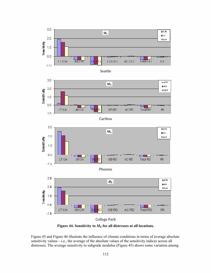
112

Seattle 

 Caribou 

Phoenix 

College Park 

Figure 44. Sensitivity to MR for all distresses at all locations.

Figure 45 and Figure 46 illustrate the influence of climate conditions in terms of average absolute sensitivity values—i.e., the average of the absolute values of the sensitivity indices across all distresses. The average sensitivity to subgrade modulus (Figure 45) shows some variation among

113

sites, but this is sensible. The highest sensitivity in Seattle is likely due to the fact that the moisture-adjusted moduli there are the lowest of the four sites. Conversely, the relatively low sensitivity of average performance to subgrade modulus for Caribou may be attributed to the frozen stiff state of the subgrade for much of the year. Subgrade conditions in Phoenix and College park are arguably intermediate between these two extremes, which is consistent with their intermediate sensitivity values. The variations in sensitivity of average performance to environmental inputs (Figure 46) are all much smaller than for subgrade modulus (Figure 45). Depths to the groundwater table, soil-water characteristic curve parameters, and saturated hydraulic conductivity all have minimal influence on the predicted pavement performance.

Figure 45. Average absolute sensitivity to subgrade MR.

Figure 46. Average absolute sensitivity to environmental variables.

0.00

0.01

0.02

0.03

0.04

0.05

0.06

0.07

0.08

0.09

Seattle Caribou Phoenix College Park

Nor

mal

ized

Sen

sitiv

ity

GWT DepthSWCClog ks

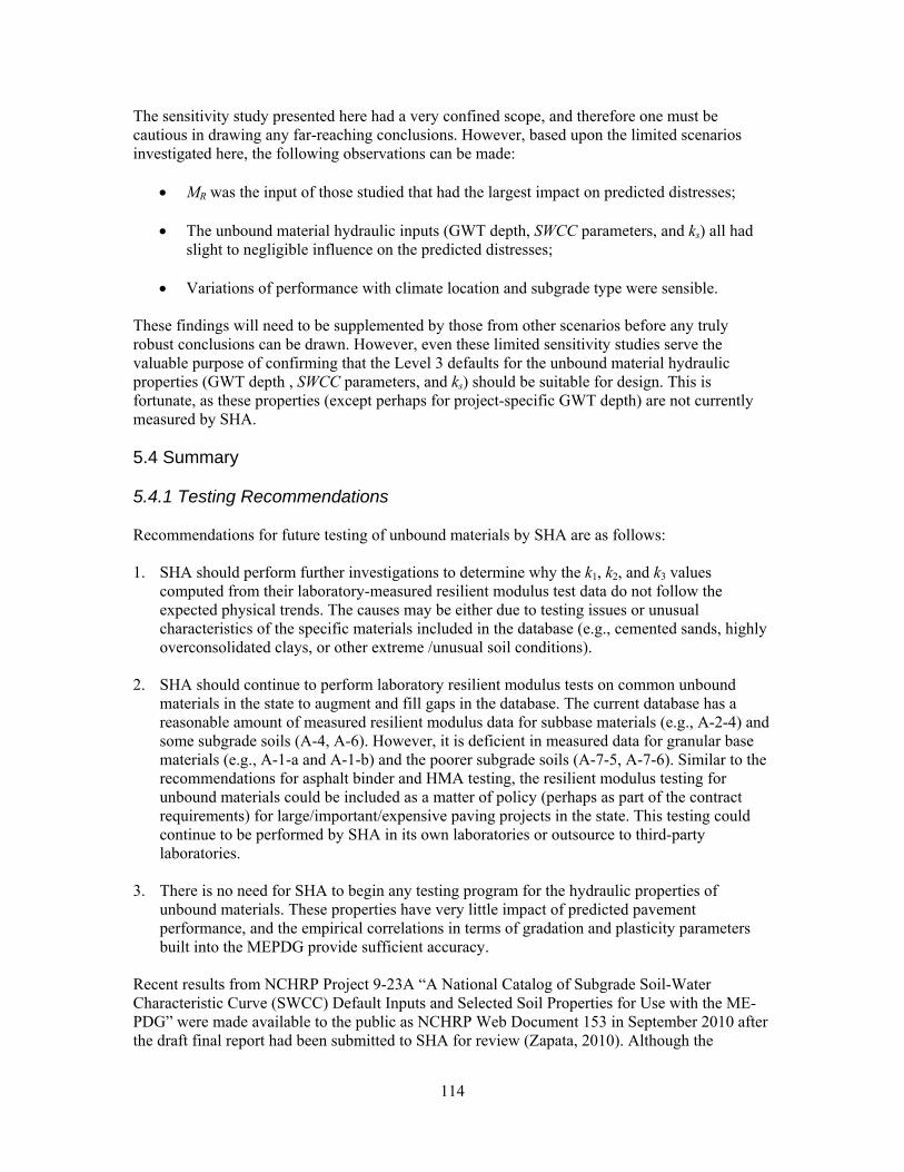
114

The sensitivity study presented here had a very confined scope, and therefore one must be cautious in drawing any far-reaching conclusions. However, based upon the limited scenarios investigated here, the following observations can be made:

• MR was the input of those studied that had the largest impact on predicted distresses;

• The unbound material hydraulic inputs (GWT depth, SWCC parameters, and ks) all had slight to negligible influence on the predicted distresses;

• Variations of performance with climate location and subgrade type were sensible.

These findings will need to be supplemented by those from other scenarios before any truly robust conclusions can be drawn. However, even these limited sensitivity studies serve the valuable purpose of confirming that the Level 3 defaults for the unbound material hydraulic properties (GWT depth , SWCC parameters, and ks) should be suitable for design. This is fortunate, as these properties (except perhaps for project-specific GWT depth) are not currently measured by SHA. 5.4 Summary 5.4.1 Testing Recommendations Recommendations for future testing of unbound materials by SHA are as follows: 1. SHA should perform further investigations to determine why the k1, k2, and k3 values

computed from their laboratory-measured resilient modulus test data do not follow the expected physical trends. The causes may be either due to testing issues or unusual characteristics of the specific materials included in the database (e.g., cemented sands, highly overconsolidated clays, or other extreme /unusual soil conditions).

2. SHA should continue to perform laboratory resilient modulus tests on common unbound materials in the state to augment and fill gaps in the database. The current database has a reasonable amount of measured resilient modulus data for subbase materials (e.g., A-2-4) and some subgrade soils (A-4, A-6). However, it is deficient in measured data for granular base materials (e.g., A-1-a and A-1-b) and the poorer subgrade soils (A-7-5, A-7-6). Similar to the recommendations for asphalt binder and HMA testing, the resilient modulus testing for unbound materials could be included as a matter of policy (perhaps as part of the contract requirements) for large/important/expensive paving projects in the state. This testing could continue to be performed by SHA in its own laboratories or outsource to third-party laboratories.

3. There is no need for SHA to begin any testing program for the hydraulic properties of unbound materials. These properties have very little impact of predicted pavement performance, and the empirical correlations in terms of gradation and plasticity parameters built into the MEPDG provide sufficient accuracy.

Recent results from NCHRP Project 9-23A “A National Catalog of Subgrade Soil-Water Characteristic Curve (SWCC) Default Inputs and Selected Soil Properties for Use with the ME-PDG” were made available to the public as NCHRP Web Document 153 in September 2010 after the draft final report had been submitted to SHA for review (Zapata, 2010). Although the

115

hydraulic properties of unbound materials have been found to have little influence on predicted pavement performance for Maryland conditions, the information in this report could be mined for additional default values if desired. Key primary information in the NCHRP 9-23A database include: AASHTO soil class; limited gradation data; Atterberg limits; saturated hydraulic conductivity; saturated volumetric water content; and volumetric water content at various levels of matric suction (used to compute soil water characteristic curve--SWCC). In addition to this primary information, there are also many secondary quantities in the database that are derived from the primary information, e.g., SWCC parameters and CBR estimated from correlations with gradation and plasticity, MR estimated from (estimated) CBR, etc. Data are organized by “map unit,” a geographical area over which the soil properties are assumed roughly uniform. There are a total of 568 map units for the state of Maryland; 79 of these have no information in the database. Of the remainder, it is expected that many will have only partial information. For example, on a national level only 66% of the map units have measured soil water characteristic curve data. Unfortunately, detailed evaluation of the Maryland data could not be performed in this study because the information became available to the public only at the very end of the project, approximately 2 months after the draft final report was submitted to SHA. 5.4.2 Recommended MEPDG Inputs The recommended unbound material inputs to the MEPDG for Maryland conditions are summarized in Table 51. Average gradation, plasticity, and volumetric information for Maryland materials as obtained from the data supplied by SHA is summarized in Table 54. The limited number of measured values for subgrade MR in Table 54 correspond to the data in Table 49 at optimum moisture and 95% compaction. Note that these values are almost all significantly lower than the MEPDG level 3 defaults and should therefore be used with caution.

116

Table 51. Recommendation material property inputs for unbound materials for Maryland conditions.

Property Input Level

Value Comment

Unbound material All Project specific Material class (e.g., AASHTO) Thickness All Project specific Strength Properties (ICM Calculated Modulus) Poisson’s ratio 3 Material specific Use level 3 defaults. Table 52 provides

additional guidance. Coefficient of lateral pressure

3 Material specific Use level 3 defaults. Table 53 provides additional guidance.

Modulus 2/3 Material specific Use level 3 defaults or values from Table 54 where available.

ICM (Mean Values) Gradation 2/3 Material specific Use values from Table 54 or level 3 defaults. Plasticity Index 2/3 Material specific Use values from Table 54 or level 3 defaults. Liquid Limit 2/3 Material specific Use values from Table 54 or level 3 defaults. Compacted All Project/layer

specific

Maximum dry unit weight

2/3 Material specific Use values from Table 54 or level 3 defaults.

Specific gravity 2/3 Material specific Use level 3 defaults. Saturated hydraulic conductivity

3 Material specific Use level 3 defaults.

Optimum gravimetric water content

2/3 Material specific Use values from Table 54 or level 3 defaults.

Degree of saturation at optimum

2/3 Material specific Use values from Table 54 or level 3 defaults.

Soil-water characteristic curve parameters (af, bf, cf, hr)

3 Material specific Use level 3 defaults.

Table 52. Typical Poisson’s ratio values for unbound granular and subgrade materials (NCHRP, 2004).

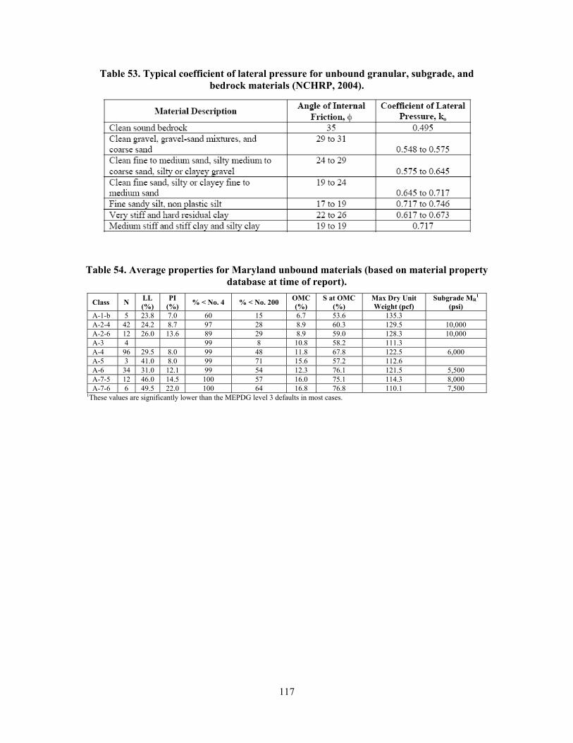
117

Table 53. Typical coefficient of lateral pressure for unbound granular, subgrade, and bedrock materials (NCHRP, 2004).

Table 54. Average properties for Maryland unbound materials (based on material property database at time of report).

Class N LL (%)

PI (%) % < No. 4 % < No. 200 OMC

(%) S at OMC

(%) Max Dry Unit Weight (pcf)

Subgrade MR1

(psi) A-1-b 5 23.8 7.0 60 15 6.7 53.6 135.3 A-2-4 42 24.2 8.7 97 28 8.9 60.3 129.5 10,000 A-2-6 12 26.0 13.6 89 29 8.9 59.0 128.3 10,000 A-3 4 99 8 10.8 58.2 111.3 A-4 96 29.5 8.0 99 48 11.8 67.8 122.5 6,000 A-5 3 41.0 8.0 99 71 15.6 57.2 112.6 A-6 34 31.0 12.1 99 54 12.3 76.1 121.5 5,500 A-7-5 12 46.0 14.5 100 57 16.0 75.1 114.3 8,000 A-7-6 6 49.5 22.0 100 64 16.8 76.8 110.1 7,500

1These values are significantly lower than the MEPDG level 3 defaults in most cases.

119

6. MATERIAL PROPERTIES DATABASE 6.1 Introduction MatProp is a MEPDG data management system based on Microsoft Access® 2007. It incorporates data entry, editing, and storing functionality for the material property inputs required by the MEPDG as well as additional data maintained by SHA. MatProp displays the data in a format similar to the MEPDG Version 1.100 data entry screens. The overall organization of MatProp is diagrammed in Figure 47.

Figure 47. Organization of MatProp database.

MatProp is composed of 3 main sections: flexible, rigid, and unbound materials. The flexible section includes both binder and HMA related data; the rigid section includes PCC related data, and the unbound section includes material property data for granular base and subgrade materials. 6.2 Instructions for Using MatProp Installation of MatProp consists of simply unzipping the “MatProp.zip” archive. This creates a folder named “MatProp System” containing 3 files: “MatProp.mdb”, the actual database; “Mouse Hook.dll,” a utility for increasing mouse functionality while within the database; and “Readme.txt,” which contains any release and/or installation notes. Double clicking “MatProp.mdb” opens MatProp. Depending upon the security settings of the host computer, the security warning shown in Figure 48 may be displayed (it may be hidden behind the main menu); if so, simply click “Options…”, choose “Enable this content” as shown in Figure 49, and click OK. After that, the main menu appears as shown in Figure 50.

Figure 48.

Figure 4

Figure

120

. Security wa

49. Security a

50. Main me

arning.

alert.

enu.

121

There are 3 buttons in the upper rectangle portion of the main menu that open screens that display the input data required by the MEPDG. Examples of these are shown in Figure 51 to Figure 55 for HMA materials after clicking “Show MEPDG HMA Input.” Note that the data display screens closely mirror the appearance of the corresponding data entry screen in the MEPDG Version 1.100. Similar MEPDG input screens are provided for the PCC and unbound material categories. The 4 buttons in the lower rectangle portion of the main menu are used for data entry and management. The data entry and management functionality for the different material categories is described in the following subsections. 6.2.1 User Interface for Flexible Pavement Material Management Clicking “Manage Binder Data” will bring up binder edit form shown in Figure 56. Binder data can be added or edited using the form in Figure 57. For consistency with the data received from SHA, the ID of binder data is numeric. Suppliers and terminals can also be added/edited/deleted as shown from Figure 58 to Figure 62. Data integrity checking is enforced as shown in Figure 63 and Figure 64. Binders can be edited by clicking “Edit” besides binder list in Figure 56 as shown in Figure 65. If “Delete” is clicked without selecting a record, a warning (Figure 66) will pop up. Clicking “Manage HMA Data” brings up the HMA data management form shown in Figure 67. New HMA mixtures can be added as shown in Figure 68. Dynamic modulus testing data can be managed as shown in Figure 69. Creep compliance data management is shown in Figure 71. If temperature is not specified beforehand, a warning will pop up as shown in Figure 70. Note that records can be excluded from calculations of average mixture properties (for a given nominal maximum aggregate size and mix type) by simply changing the “excluded” control to “Yes”.

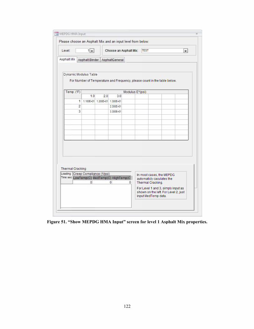
F

Figure 51. “SShow MEPDDG HMA Inp

122

put” screen foor level 1 Aspphalt Mix pr

roperties.

F

Figure 52. “Shhow MEPDGG HMA Inpu

123

ut” screen forr level 2/3 Assphalt Mix p

properties.

Fig

gure 53. “Shoow MEPDG HMA Input

124

” screen for level 1/2 Aspphalt Binder

properties.

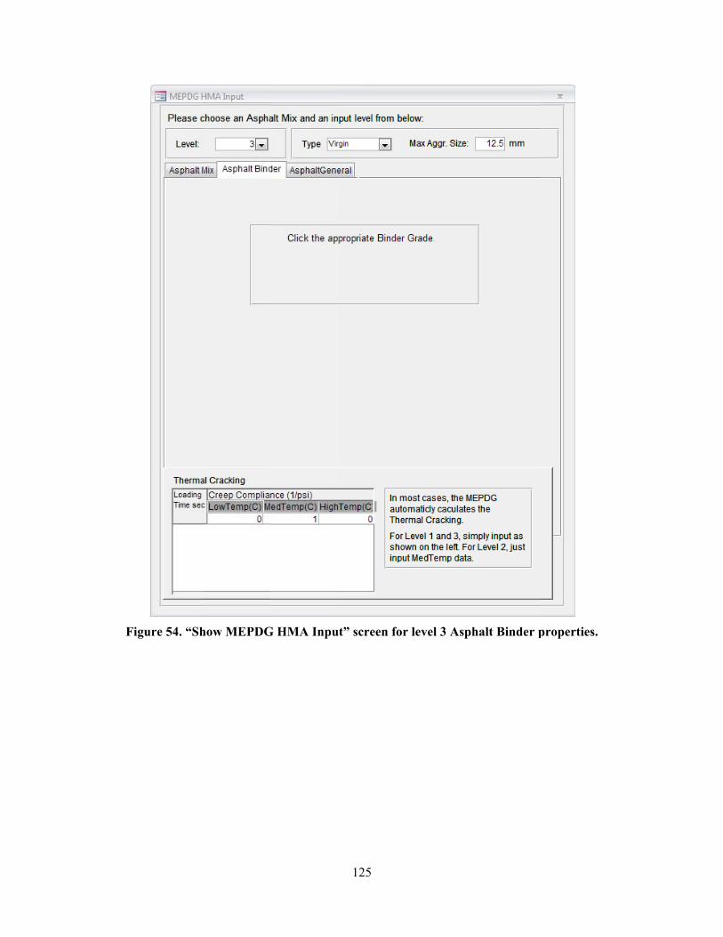
Fi

igure 54. “Shhow MEPDGG HMA Inpu

125

ut” screen forr level 3 Asphhalt Binder p

properties.

Figuure 55. “Show MEPDG HHMA Input”

126

” screen for Alevels).

Asphalt Geneeral properti

ies (all input

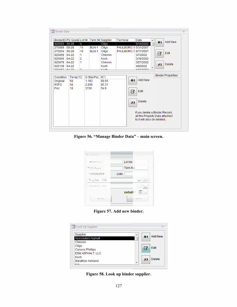
Figure 5

F

56. “Manage

Figure 57

igure 58. Loo

127

Binder Data

7. Add new bi

ok up binder

a” – main scr

inder.

r supplier.

reen.