cash flow risk management – in good times and bad of!financialrisks! to! their cash! flow! in!...
TRANSCRIPT

ERM Symposium 2011 – Chicago, IL – March, 2011 1
Abstract – Non-‐financial businesses face a variety of financial risks to their cash flow in good times, but in times of extreme economic volatility, proper risk management can mean the difference between survival and bankruptcy. This paper will review a variety of risk management theory that deals with correlated, non-‐normally distributed factors, and then apply risk management techniques to the U.S. steel industry using futures contract hedging that reduces a company’s risk and increases profit during the worst part of the 2007-‐2009 recession.
Keywords: supply and demand shocks, futures derivatives, optimal hedging, U.S. steel industry, filtered historical simulation, GARCH(1,1)
1. The Need for Risk Management When profits are consistently high, executives often find it difficult to justify taking measures that reduce the potential for loss. The logic goes that the longer the company remains profitable, the less likely a period of loss or sustained loss will occur. Nothing could be further from the truth.
To manufacturing companies, losses occur when revenues are lower than expenses.
Π = !"#$%& = !"#"$%" − !"#$%&$& = ! − ! (1)
!. !. ! > !
ℒ = !"## = !"#"$%" − !"#$%&$& = ! − ! (2)
!. !. ! < !
In general, a company can go from profit to loss if:
1. revenues decrease faster than expenses,
!! > !!!! ,!"!"> !"
!" (3)
2. or expenses increase faster than revenues.
!! < !!!! ,!"!"< !"
!" (4)
In practice, revenues and expenses are dependent on internal and external factors. Assuming companies can control their internal factors, the primary risks to the company are posed by external factors, or shocks.
When a demand shock causes revenue to fall faster than expenses (3), a manufacturing company has few options beyond borrowing to cover expenses or seeking bankruptcy to lower expenses.
When a supply shock causes expenses to rise faster than revenue (4), a manufacturing company may be able to raise its prices, but this risks lowering demand and offsetting any expected revenue increase.
In times of severe economic volatility, expenses may rise and revenues may fall simultaneously -‐ due solely to external factors outside of a company’s control. Only the strongest of the industry’s firms may survive.
During the 2007-‐2009 recession, the U.S. auto industry saw the first ever bankruptcies of two of the “Big Three” automakers. It was only through the direct takeover of GM and Chrysler by the US government did they manage to avoid liquidation and re-‐emerge from bankruptcy in 2010. After suffering an indirect supply shock of rising oil prices that caused their customers to shift from their large, fuel-‐inefficient vehicles to more fuel-‐efficient ones sold by their foreign rivals, GM and Chrysler suffered a severe demand shock when the U.S. economy entered its worst recession since the 1930s. By 2008, light vehicle sales in the United States had fallen to just over 9 million – down from 17 million in 2006. [Figure 1]
[Figure 1]
Cash Flow Risk Management – in good times and bad
Anthony (Tony) Sabbadini with Michael Lim

2 ERM Symposium 2011 – Chicago, IL – March, 2011 The supply shock effect of a rising oil price not only affects the auto industry, but all facets of the transportation sector – none more acutely than the airline industry. From 1979 to 2009, 42 airlines in the United States declared bankruptcy.1 Of those, only 3 airlines went bankrupt when the price of oil was below the long run average price from 1869 to 2009, computed in 2008 dollars. By far most bankruptcies occurred during periods of high or rising oil prices. [Figure 2]
[Figure 2]
In both the auto and airline industries, however, success stories stand out as examples of prudent risk management. In the case of Ford, America’s other “Big Three” automaker, and the only automaker not to go bankrupt and take federal bailout assistance, success can be attributed to a recognition in 2009 that its heavy debt load would bring bankruptcy if the US economy took another downturn, and a concrete debt reduction plan coupled with a built-‐in cash cushion. The result was an increase in its credit rating and a decrease in its subsequent borrowing costs.2
Southwest Airlines stands out among U.S. carriers as perhaps the most “aggressive hedger” when it comes to managing the risk of a rising price of oil (and in turn a rise in the price of crude-‐oil derived kerosene jet fuel.) In the third quarter of 2005, only 4 weeks after rival Delta Airlines had declared bankruptcy – citing rising fuel costs as a major reason3 -‐ Southwest reported a $227 million profit. What is particularly interesting to note is the airline also posted $295 million gain from its “successful hedging
1 http://en.wikipedia.org/wiki/Airline_bankruptcies 2 ‘The road back to investment grade: Ford Motor’, Treasury & Risk: 36: November, 2010 3 http://en.wikipedia.org/wiki/History_of_Delta_Air_Lines#Bankruptcy
program” against higher prices. In other words, Southwest would have incurred a $68 million loss if it had gone unhedged.4
Risk management programs, however, are not without their costs. During times of extreme economic volatility, hedges placed against a rise in prices may result in a loss as prices decline. But if hedging is done properly, lower expenses offset this loss -‐ e.g., lower jet fuel costs. Nonetheless, executive management is often tempted to scale back hedging programs that are currently out-‐of-‐the-‐money. In August 2008, US Airways ended its jet fuel hedging program, with prices of crude oil at around $60 a barrel. No doubt they imagined prices to continue their relatively low levels compared to the previous year, as the US economy entered the depths of its 18-‐month recession. Their timing could not have been worse. Almost immediately, prices proceeded to rise, reaching $90 a barrel within a year. At the time, Southwest had maintained its hedging program, citing “a philosophy of managing the business against catastrophic fuel prices.” Indeed, hedging is not meant to guarantee profits, but rather as an insurance policy against catastrophic loss.5
Predicting catastrophic supply or demand shocks, however, is extremely difficult. Quantitative techniques employing heavy application of statistics and computational power to forecasting prices and calculating risk is no guarantee against catastrophic loss, and can only serve as a supplement to a carefully constructed risk management program. In fact, overreliance on popular quantitative tools such as Economic Capital (EC) or Value at Risk (VaR) can lead to increased risk of catastrophic loss.6
A major problem lies in the pro-‐cyclical nature of these tools. During good times, the historical data used to estimate the probability of a downturn includes fewer and fewer bad days. This can lead managers to a false sense of security, and encourage them to take on more risk in the form of debt or enter less profitable or more volatile markets. This makes a company all the more vulnerable when markets turn against it.
The reality is, few if any people can truly predict a catastrophic downturn such as the one that brought the US housing market and banking sector to its knees in the 2007-‐2009 recession. The only thing companies can do is be prepared for when the inevitable downturn occurs. This requires long-‐term thinking on the part of management, and an appropriate set of risk management tools. This paper will offer one such approach. 4 ‘Southwest Hedging Fuels Q3 Results’, CFO.com, Oct. 21, 2005 5 ‘US Airlines rue hedging programs’, Global Markets, Aug. 2, 2010 6 ‘2009 Federal Reserve Bank of Chicago Annual Report’

ERM Symposium 2011 – Chicago, IL – March, 2011 3
2. The Tools of Risk Management The oldest form of managing risk is simply not to take it. If a house in on fire, don’t walk into it. Technically, this is called risk avoidance. But in practice, few risks are completely avoidable, and fewer still are as obvious to avoid as a burning house. The reality is that in order to make a profit, let alone exist, companies must take some risk in order to achieve their objectives. As such, companies must look beyond simple risk avoidance.
Perhaps the second oldest form of risk management is saving. Setting aside assets in good times to survive the bad times – the proverbial “rainy day fund.” Savings can be practiced in countless different ways, ranging from collecting firewood in the summer to burn during the winter, all the way to holding demand deposit accounts in various offshore banks, guaranteed by a patchwork of private and government-‐backed insurance schemes. Regardless of the form and level of sophistication, savings can and should be part of any risk management program, and goes a long way towards avoiding the problems caused by overleverage that have bankrupted many financial and non-‐financial firms alike during times of economic distress.
A third tool of risk management is diversification. By taking a portfolio approach to income streams as opposed to relying on a single source, companies can expect that weakness in one part of the portfolio be partially offset by another’s relative strength. The question then is what combination of income streams is appropriate for a given company’s risk tolerance.
[Figure 3]
In a purely financial portfolio, Modern Portfolio Theory7 (MPT) attempts to answer this by calculating the expected return E r and expected volatility E[!!] of different combinations of income streams. It can be shown that certain combinations have both lower E r and E[!!], and are thus deemed inferior and removed from further consideration (assuming investors seek higher returns and
7 Markowitz, Harry, ‘Portfolio Selection’, Journal of Finance, 1958
lower volatility.) The remaining combinations are referred to as the “efficient frontier” [Figure 3]. This filtering helps reduce the complexity of deciding where to allocate income streams, but it does not solve it. Investors must still decide what level of risk and return are preferred.
In a manufacturing portfolio, MPT can be applied to selecting a company’s product mix (output) or proportion of raw materials (input) within a volatility framework, saving on factory startup/shutdown costs.8 In certain businesses, the ability to change input and output characteristics is relatively easy, such as in some food and beverage products – swapping sugar with corn syrup, for example. But in other manufacturing businesses, firms are not able to freely adjust the proportion of their income streams as one would in a financial portfolio.
The main reason is that in manufacturing, product mix, raw materials and fixed-‐capital requirements are often constrained by strict product engineering specifications. In other words, few automobile manufacturers can simply swap out overnight their steel car body designs for aluminum ones when the price and volatility characteristics of spot aluminum become favorable. In reality, these design and manufacturing changes can take years of careful planning. For this reason, most manufacturing companies seek to offset the risk exposure of their current product mix using carefully tailored financial hedges.
3. An Introduction to Hedging A primary function of financial markets is to enable the efficient transfer of risk. Parties seeking to reduce their risk level can trade a variety of financial instruments that allow other parties to take the downside of price changes in exchange for the opportunity to profit from the upside.
The classic example of this exists in the forward contract. Imagine that a wheat farmer in the American Midwest is concerned about the chance of a good growing season creating a surplus of supply in the grain markets, thereby depressing prices he will receive when he goes to sell his harvest. In order to lock in a profitable budget for planting his crop, hiring help, and leasing the necessary farming machinery, the farmer calls a grain merchant and agrees to sell forward his wheat crop at a set date for an agreed upon price.
This forward contract removes the risk to the farmer that market price declines will force him to sell his crop unprofitably – but it also precludes the possibility of
8 Sabbadini, Tony, ‘Manufacturing Portfolio Theory’, InterSymp 2010

4 ERM Symposium 2011 – Chicago, IL – March, 2011 market price rises increasing the value of his crop. The grain merchant, in contrast, takes the opposite side of the trade. Concerned about a rise in prices, the grain merchant no longer carries the risk that the price she will pay this farmer will go up if the market price subsequently rises. Just like the farmer, however, she is limited on the upside. In her case, the merchant will not be able to take advantage of falling market prices. In effect, the two parties have traded each other’s upside potential in exchange for downside protection.
The basic principles illustrated in the preceding example form the basis for what is at the heart of all financial hedging transactions. Hedging exists to serve already functioning marketplaces composed of buyers and sellers, but adds the ability to manage risk. In the case of a buyer, she is concerned about an increase in price. As such, she is naturally “short”, and seeks to hedge her price risk by going “long” with an appropriate financial instrument and counterparty. Because of the difficulty of finding a counterparty that is willing to trade risk with her in her location at a reasonable price for her particular grade of product, the buyer will often go to a standardized futures and options derivative exchange such as the Chicago Board of Trade (CBOT). As the oldest futures and options exchange in the world, the CBOT, now part of the larger Chicago Mercantile Exchange (CME) Group, functions as a central meeting place for buyers and sellers of risk to:
1. find each other (matching)
2. trade at a market price (price discovery)
3. trade at a desired quantity (liquidity)
4. trade at a standardized quality (grading)
5. trade without concern for the counterparty defaulting on their obligations (clearing)
For these reasons and more, global futures and options markets on exchanges like the CBOT reached a total trading volume of over 17.7 billion contracts in 2009.9 Of the major financial instrument classes, futures contract trading comes second only to the foreign exchange currency spot market on a per instrument, average volume basis in the U.S. market, surpassing equity options, stocks, and bonds.10
In the US markets alone, futures contracts covering products ranging from corn and soybeans, crude oil and natural gas, gold and silver, copper and zinc, U.S. Treasury bonds, and a variety of foreign exchange
9 ‘Volume Trends’, Futures Industry, March 2010 10 ‘Harris, Larry, ‘Trading and Exchanges’, pg. 45, Oxford Press, 2003
currency pairs such as the Swiss Franc to Japanese Yen and the U.S. Dollar to British Pound have been trading with high volume for several decades. More recently, the New York Mercantile Exchange (NYMEX) (owned by CME) introduced the Hot Rolled Coil (HRC) steel futures contract, which will be the subject of this paper’s case study on risk management in the U.S. steel industry. This breadth of products allows financial and non-‐financial firms alike to manage the three primary forms of market risk:
1. price risk
2. interest rate risk
3. foreign exchange risk
Of the Dow Jones Industrial Average constituent “blue chip” 30 companies representing large, prominent publicly traded firms based in the United States, all of them make extensive use of financial derivatives, ranging from interest rate and currency swaps, options, and forwards to commodity futures.11
The breadth and depth of the financial derivatives marketplace makes it both powerful and relatively efficient -‐ yet simultaneously daunting. Choosing a trading strategy composed of price and volume conditions, order types, and various broker-‐dealers and clearing firms connecting you to derivatives exchanges is a full time job. Navigating the sheer number of contract types alone can take months of careful study. And designing a hedging strategy that aligns with company goals requires careful study of the individual business and an analysis of appropriate financial hedging instruments. This process is unique for every business examined. But an overall framework -‐ incorporating the best practices of the risk management field -‐ is needed in order to reduce research time, errors, and ultimately, risk.
4. Cash Flow Risk Management Businesses seek to maximize profit.
!"# Π = !"#(! − !) (5)
This further decomposes to:
!"# Π = !"# ! ,!"#(!) (6)
Unfortunately, revenue and expenses cannot be optimized separately, as they share terms. For a single-‐product firm:
profit = Π = ! − ! = ! ∗ !! − ! ∗ (!! +!") − !" (7)
11 Dr. Gary Giroux, http://acct.tamu.edu/giroux/, Texas A&M

ERM Symposium 2011 – Chicago, IL – March, 2011 5 Where Q is quantity produced, !! is the price of output, !! is the price of input, MC is the marginal cost, and FC is fixed costs (e.g., depreciation on capital equipment, etc.). Setting aside FC, cash flow = ! = Π + FC, and is a function of these four main components in the short run:
π = !(!,!!,!! ,!") (8)
The objective functions are, ceteris paribus:
!"# π,!! , !"# !! (9)
MC is typically modeled in classical microeconomic theory as a function of Q, representing increasing costs of each marginal unit produced (i.e., diminishing returns). But generally, this property is not always present in certain businesses such as software, where the production cost does not change with each incremental unit produced. Thus, it is can be viewed as a constant, zero, or a function of other variables, and does not have a general objective function. For quantity:
!"# ! (10)
!. !. !! − !! −!" > 0 ELSE Q = 0
Assuming a competitive market, the only variable a company has direct control over in the short run is Q, and is always maximized until (10) is no longer satisfied. Eventually, !! +!" = !! , and further production is no longer profitable -‐ or all demand is satisfied -‐ and production stops.
Extending this notion to the market, where all companies in the industry sell their goods to a public that buys more at a lower price and less at a higher price, the market price for goods is determined by the intersection of supply and demand curves reflecting these incentives.
The simplest example would be a two-‐company industry composed of firm ‘a’ and firm ‘b’. Each company has its own production costs and corresponding output:
Which, in the case where there is a linear demand equation of D = 12 – P, the market clears at a price (Po) of 4.5, as illustrated in Figure 4, period 1. In supply-‐demand graphs:
price (P) is on the vertical axis quantity (Q) is on the horizontal
[Figure 4]
The two firms ‘a’ and ‘b’ individual supply curves are the dashed ‘a’ and dotted ‘b’ lines, respectively, and they combine to form the industry total ‘t’. The ‘t’ curve intersects with the ‘demand’ curve at the diamond to form the industry-‐clearing market price (Po). The firms then sell their products until they reach the market price, and their respective production amounts are shown on their supply curves, denoted by the square for firm a and the circle for firm ‘b’.
[Figure 5]
From a risk management standpoint, this framework becomes useful when analyzing the impact of various shocks to the system.

6 ERM Symposium 2011 – Chicago, IL – March, 2011
Taking the U.S. auto industry again, the fall in sales during the 2007-‐2009 recession can be viewed as a demand shock in period 2 [Figure 5], shifting the demand curve down. As customers demand less, the market price and quantity each firm produces drops – as does profit.
The U.S. airline industry prior to the 2007-‐2009 recession experienced a supply shock as oil prices rose. In our framework, Pi shifted up [Figure 6].
[Figure 6]
As airlines cut their newly unprofitable routes, quantity supplied goes down, the price of airfare goes up, and each airline’s flight time decreases.
[Figure 7]
The question is what if one airline managed to hedge their costs, just like Southwest did successfully throughout the early to mid 2000s? The result in our framework is the hedged airline becomes more profitable and flies more. Its competitor makes less money and flies less -‐ just as many of Southwest’s competitors.
The effect of the hedge can be seen in Figure 7. As the supply shock sends the cost of production, Pi, up to 3 for company ‘b’, the firm a’s hedge offsets the increase in Pi and allows firm a to continue producing at Pi = 2. Visually, this shows up in the kinked ‘t’ (total) supply curve as firm ‘a’ is the only producer until its MC + Pi = 3, when firm ‘b’ starts producing as well. The actual results are:
Hedging, however, is not a guarantee of profits. A company can lose money from hedging as well. If, instead of Pi shifting up, Pi shifts down – a company like ‘a’ which had hedged against rising prices would lose money from the hedge, offsetting any benefits of the price decrease.
[Figure 8]
In effect, company ‘a’ has its original cost structure – the goal of the hedge – but its competitors have a lower cost structure. So why bother with hedging at all if it cannot guarantee higher profits? The answer is the cost of volatility. Done correctly, hedging reduces volatility.

ERM Symposium 2011 – Chicago, IL – March, 2011 7
5. Motivating the Hedge Reduction in cash flow volatility increases firm value. Several research papers illustrate how hedging reduces corporate taxes12, increase debt capacity13, and enables firms to take advantage of new investment opportunities (by, for example, not having a budget that is stripped of surplus capital due to excessive losses.) In the airline industry, this effect is estimated to increase firm value by 5 to 10%14. [Figures 9, 10: unhedged vs. hedged]
[Figure 9: unhedged]
[Figure 10: hedged]
Perhaps the simplest way to understand how hedging benefits firms is to consider the risk of bankruptcy. Even if in the long run a company breaks even, creditors may eventually refuse to lend to cover losses [Figure 11].
[Figure 11: unhedged]
12 Graham and Smith, ‘Tax Incentives to Hedge’, 1998 13 Graham; Rogers, ‘Does Corporate Hedging Increase Firm Value?’ 2000 14 Carter, et. al. ‘Does Hedging Affect Firm Value?’, 2006
Proper hedging reduces volatility, smoothing cash flow into an acceptable range [Figure 12]. Notice that over time, hedged cash flow is roughly equal to without hedging.
[Figure 12: hedged]
Thus, the measure of an effective hedging program is its reduction in volatility compared to the unhedged case.
6. Designing the Optimal Hedge A perfect hedge will reduce the volatility, measured as the standard deviation of an income stream (original + hedge position return), to zero. Perfect hedges are found in markets where the traded good being hedged is interchangeable with the hedging good. In futures markets, this means that the spot and future market prices converge upon contract expiration, and the purchaser can take delivery of the underlying asset to use as she would if she had instead purchased it on the spot market.
Often times, however, the hedger cannot or does not wish to use the deliverable grade of the underlying future contract asset, and simply offsets the contract before expiration. An airline hedging kerosene prices, for example, would typically offset their long futures position in crude oil without ever taking delivery. In effect, they are using the future contract as a cross hedge.
Cross hedges vary from simple, intuitive relationships -‐ such as those found in the transportation fuels markets – to complex and non-‐intuitive hedges composed of baskets of seemingly unrelated commodities and non-‐linear derivatives such as options. It is our experience that such “advanced” hedging strategies can be unstable, and only perform under precise assumptions about market conditions such as a normal Gaussian distribution of returns. Thus, in this paper we examine several relatively simple approaches to designing an effective hedge, and focus on reliability and protection from loss instead of marginal improvements in volatility reduction that perform only under prescribed scenarios.
To find such a robust and effective hedging strategy, we examine the U.S. steel industry.

8 ERM Symposium 2011 – Chicago, IL – March, 2011
7. The U.S. Steel Industry Steel is an old product. Known to have been made for over 3000 years, carbon steel (the most basic steel alloy between carbon and iron) has applications today in some of the most essential products in the modern economy, ranging from rail tracks, structural beams, car bodies, containers, and more. Worldwide, steel production reached over 1.4 billion metric tons in 2010.15
In the United States, steel has a long and storied history. It played a pivotal role in the construction of the great skyscrapers of Manhattan and Chicago, the building of the transcontinental railroad, the Hoover Dam, the Golden Gate Bridge, and of course the body of the first truly affordable passenger automobile, the Ford Model T. Without steel, the United States would arguably not have taken the helm as home to the world’s largest corporations in the 20th century. After all, the first billion-‐dollar company was formed in 1901 with the creation of U.S. Steel Corporation by J.P. Morgan’s merging of Carnegie Steel with the Federal and National steel companies.
U.S. Steel still exists today – perhaps as a testament to its great legacy. But since the late 1950s, the U.S. steel industry has undergone tremendous structural and secular decline, partly as post-‐war Europe and Japan emerged as fierce global competitors, but also because of outdated technology and strategy, legacy pension costs, and poor labor-‐relations. Beginning in the 1960s and spiking in the 1970s and early 2000s, large-‐scale bankruptcies of 50 to 100 year old firms occurred, culminating in the closure of Bethlehem Steel Corporation in 2003 – the very company that had provided the steel for the Hoover Dam and the Golden Gate Bridge.
[Figure 13]
Despite this volatility, the steel industry has until recently lacked a futures market for managing price risk. Perhaps because of it’s long history, steel companies have traditionally preferred to deal with customers and suppliers using long-‐term contracts at privately negotiated prices. This is changing, however, as steel firms demand
15 http://www.worldsteel.org/?action=newsdetail&id=319
more price transparency as prices of iron ore and finished goods such as hot rolled coil fluctuate. [Figure 13]
Of the commodities markets, steel is the second largest after crude oil, and is 15 times the size of all other metals markets combined -‐ and twice their value.16 Of these “lesser” metals, including such important commodities as copper, zinc, and aluminum, developed futures markets exist. Alcoa, America’s largest aluminum producer, uses futures and other derivatives extensively to hedge its price risk in aluminum. The LME aluminum futures contract serves as a direct hedging instrument, as well as a benchmark for other hedging derivatives.17
In fact, the LME now offers a steel billet futures contract that, after a slow start, has picked up considerable momentum, trading over 10 million metric tons in 2010. However, the world leader in steel futures trading, the Shanghai Futures Exchange (SHFE), dwarfs all others, with 180 million contracts traded in 2010. [Figure 14]
[Figure 14]
Unfortunately, the SHFE is only available to Chinese commercial hedgers and retail investors, and lacks delivery points outside of China. Another concern for U.S. steel makers is that the LME billet contract was recently reconfigured, and went from a fairly high correlation of 94% (good) with scrap metal prices – to 64% (poor).18 Thus, we focus in this paper on the U.S. Midwest Hot Rolled Coil (HRC) Steel Index futures, traded at the CME.
16 Joanne Morrison, ‘Steel Futures Forge Ahead’, Futures Industry, 1/2011 17 Dr. Gary Giroux, http://acct.tamu.edu/giroux/, Texas A&M 18 Michael Marley, ‘Scrap companies are still up for grabs, but no megadeals’ American Metal Market, 10/2010

ERM Symposium 2011 – Chicago, IL – March, 2011 9
8. Developing a Hedge for Steel Before we settled on the HRC futures contract as our principal risk management tool for a model of a U.S. steel company selling hot rolled coil, we considered a wide variety of possible cross hedges that might serve as a hedge against various economic shocks to steel prices and other factors important to making this type of steel. In short, we find a relatively simple approach performs best.
One of the approaches we tried was using a basket of futures contracts to hedge the volatility of important factors. DeMaskey19 develops this approach for finding the optimal number of a basket of currency future contracts to hedge the spot price of a different currency. While she was able to show that a basket of currency cross hedges was better than a single cross hedge, both performed worse (i.e., had higher volatility) than an unhedged position in the spot currency. Our preliminary results testing a basket of non-‐ferrous cross hedges (Japanese Yen, copper, etc.) revealed similar results: the baskets were better than individual cross hedges, but all basket hedges performed worse than unhedged case. It was our single-‐instrument, direct hedge using HRC futures that performed the best.
Take copper futures cross hedge, which has an 85% correlation with the scrap steel price20. [Figure 15]
[Figure 15]
Hedging with copper increased volatility (by 15%) compared to the unhedged case. Profits do increase, but at the expense of higher risk. This is speculation. Risk-‐adjusted, the hedge performed only marginally better, as measured by the Sharpe Ratio21 (S = Π/σ). [Figure 16]
19 Andrea DeMaskey, ‘Single and Multiple Portfolio Cross-‐Hedging with Currency Futures’, Multinational Finance Journal, 1997 20 CRB: No. 1 Heavy Melting Scrap, Chicago 21 http://en.wikipedia.org/wiki/Sharpe_ratio
[Figure 16]
Despite the increase in risk from copper future hedging, relatively speaking, it was one of the best cross hedges we tested. Other hedges we examined fared much worse, such as those with currency futures. Figure 17 shows the wide divergence in movements and volatility, especially that inherent in emerging markets.
[Figure 17]
When we did settle on a few promising hedge candidates, we noticed that using the naïve hedge ratio – i.e., taking an exactly equal number of offsetting contracts to the natural position – performed poorly compared to the minimum variance hedge.
[Figure 18]
Notice that the naïve copper hedge Figure 18 has a very large downside spike in 2006, resulting in a net loss.

10 ERM Symposium 2011 – Chicago, IL – March, 2011 Volatility is also higher than the unhedged case [Figure 19].
[Figure 19]
This happens because the naïve hedge is not adjusting to underlying changes in the correlation between scrap and copper prices, resulting in poorly positioned hedges. The correlation does stay within a trading range and, over the long run, appears somewhat stable, but nonetheless, the 1-‐year moving average of the correlations indicates there are times of extreme divergence from trend, and thus the resulting extreme losses on net profit [Figure 20].
[Figure 20]
To address this shortcoming, as well as the possible divergence over time in relative volatilities of the spot and futures prices, we employed a minimum variance hedge22 using a 1-‐year moving average of the natural logarithm of the monthly average prices (roughly equivalent to the monthly percentage change).
ℎ∗ = −1 ∙ !!,! ∙!!!! (11)
Where ℎ∗ is the optimal hedge ratio, !!,! is the correlation between the spot and future returns [ln(pricet/pricet-‐1)], !! is the standard deviation of the spot returns, and !! , the standard deviation of the future returns. The -‐1 is the inverse relationship a hedge has to the underlying spot position, offsetting a natural long position with a short, and vice-‐versa, assuming a positive correlation coefficient. Then, (12) shows how many contracts with which to hedge.
22 Luenberger, David G., ‘Investment Science’, 2009, Oxford Press, p. 283
!∗ = ℎ∗ ∙ !!!!∙!!
(12)
Where !∗ is the optimal number of futures contracts, !! is the cash flow of the natural spot position, !! is the price of the futures contract, and !! is the number of units of the underlying commodity in the futures contract, per contract (the HRC contract, for example is 20 tons.)
Furthermore, because we utilize a 1-‐year moving average of monthly prices, we implement a rolling hedge, maintaining an open position in 12 contracts of staggered maturity date 1 to 12 months out. Each month we close the contracts nearing expiration and book profits. Thus:
!!∗ = ℎ!∗ ∙!!,!
!!,!∙!!,!∙!"!!!!!!" (13)
Where !!∗ is the total number of rolling contracts outstanding at time t, and the other variables, as previously defined, for their respective time period i.
9. Hedging Results Using the approach outlined in (11-‐13), and staying away from tenuous cross hedges such as copper because of our preliminary results and other authors’ research23, we hedged the cash flow of a hypothetical U.S. based HRC steel producer, modeled after Nucor, from 2001 through July 2009, using HRC futures. Nucor, being a mini-‐mill operator that uses electric-‐arc furnaces to melt scrap metal into finished products, pays approximately 40-‐50% of its final product price towards the cost of scrap.
The remainder of its variable cost is in labor, electricity to run the furnaces, and general administrative sales and overhead. Most mini-‐mills operate on a flexible work arrangement, whereby the workers are paid only when the plant is operational – in stark contrast to some of the unionized integrated mill operators. Since the price of semi-‐skilled labor is fairly stable and usually benchmarked off the minimum wage, labor cost risk is relatively low for mini-‐mill operators.24
Turning to electricity price volatility, opaque over the counter (OTC) markets do exist for energy trading using swaps and other complex derivatives, but due to multiple cases of market failure and manipulation throughout the early 2000s by firms such as Enron, the electricity derivatives market remains largely closed to commercial hedgers and is tightly regulated. Despite being locked out of the hedging market, commercial users of electricity do enjoy the advantage of relatively stable 23 Dhuyvetter, et. al. -‐ 'Cross Hedging Agricultural Commodities' -‐ Kansas State University -‐ Agricultural Experiment Station and Cooperative -‐ 1997 24 'Iron & Steel Manufacturing in the US', IBIS World Industry -‐ 7/2010
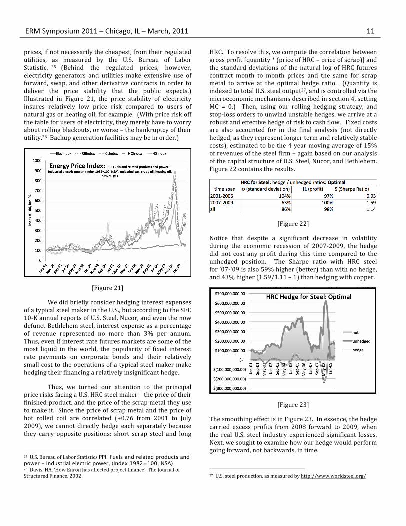
ERM Symposium 2011 – Chicago, IL – March, 2011 11 prices, if not necessarily the cheapest, from their regulated utilities, as measured by the U.S. Bureau of Labor Statistic. 25 (Behind the regulated prices, however, electricity generators and utilities make extensive use of forward, swap, and other derivative contracts in order to deliver the price stability that the public expects.) Illustrated in Figure 21, the price stability of electricity insures relatively low price risk compared to users of natural gas or heating oil, for example. (With price risk off the table for users of electricity, they merely have to worry about rolling blackouts, or worse – the bankruptcy of their utility.26 Backup generation facilities may be in order.)
[Figure 21]
We did briefly consider hedging interest expenses of a typical steel maker in the U.S., but according to the SEC 10-‐K annual reports of U.S. Steel, Nucor, and even the now defunct Bethlehem steel, interest expense as a percentage of revenue represented no more than 3% per annum. Thus, even if interest rate futures markets are some of the most liquid in the world, the popularity of fixed interest rate payments on corporate bonds and their relatively small cost to the operations of a typical steel maker make hedging their financing a relatively insignificant hedge.
Thus, we turned our attention to the principal price risks facing a U.S. HRC steel maker – the price of their finished product, and the price of the scrap metal they use to make it. Since the price of scrap metal and the price of hot rolled coil are correlated (+0.76 from 2001 to July 2009), we cannot directly hedge each separately because they carry opposite positions: short scrap steel and long
25 U.S. Bureau of Labor Statistics PPI: Fuels and related products and power - Industrial electric power, (Index 1982=100, NSA) 26 Davis, HA, 'How Enron has affected project finance', The Journal of Structured Finance, 2002
HRC. To resolve this, we compute the correlation between gross profit [quantity * (price of HRC – price of scrap)] and the standard deviations of the natural log of HRC futures contract month to month prices and the same for scrap metal to arrive at the optimal hedge ratio. (Quantity is indexed to total U.S. steel output27, and is controlled via the microeconomic mechanisms described in section 4, setting MC = 0.) Then, using our rolling hedging strategy, and stop-‐loss orders to unwind unstable hedges, we arrive at a robust and effective hedge of risk to cash flow. Fixed costs are also accounted for in the final analysis (not directly hedged, as they represent longer term and relatively stable costs), estimated to be the 4 year moving average of 15% of revenues of the steel firm – again based on our analysis of the capital structure of U.S. Steel, Nucor, and Bethlehem. Figure 22 contains the results.
[Figure 22]
Notice that despite a significant decrease in volatility during the economic recession of 2007-‐2009, the hedge did not cost any profit during this time compared to the unhedged position. The Sharpe ratio with HRC steel for ’07-‐‘09 is also 59% higher (better) than with no hedge, and 43% higher (1.59/1.11 – 1) than hedging with copper.
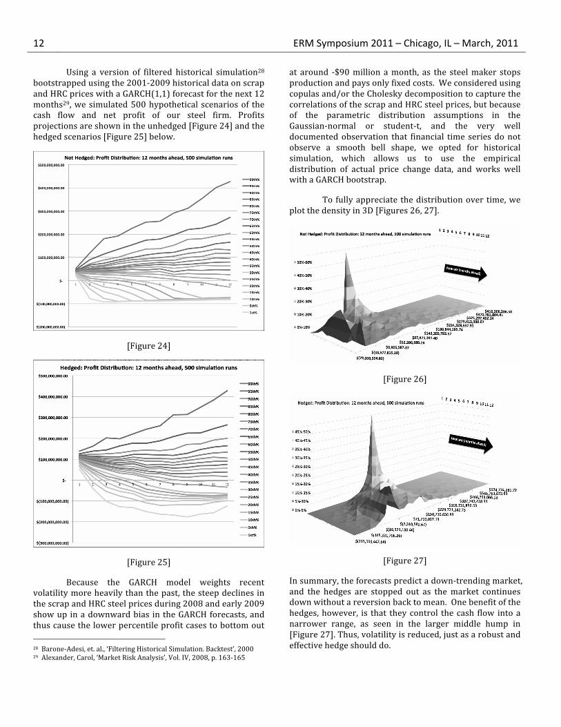
[Figure 23]
The smoothing effect is in Figure 23. In essence, the hedge carried excess profits from 2008 forward to 2009, when the real U.S. steel industry experienced significant losses. Next, we sought to examine how our hedge would perform going forward, not backwards, in time.
27 U.S. steel production, as measured by http://www.worldsteel.org/
12 ERM Symposium 2011 – Chicago, IL – March, 2011 Using a version of filtered historical simulation28 bootstrapped using the 2001-‐2009 historical data on scrap and HRC prices with a GARCH(1,1) forecast for the next 12 months29, we simulated 500 hypothetical scenarios of the cash flow and net profit of our steel firm. Profits projections are shown in the unhedged [Figure 24] and the hedged scenarios [Figure 25] below.
[Figure 24]
[Figure 25]
Because the GARCH model weights recent volatility more heavily than the past, the steep declines in the scrap and HRC steel prices during 2008 and early 2009 show up in a downward bias in the GARCH forecasts, and thus cause the lower percentile profit cases to bottom out 28 Barone-‐Adesi, et. al., ‘Filtering Historical Simulation. Backtest’, 2000 29 Alexander, Carol, ‘Market Risk Analysis’, Vol. IV, 2008, p. 163-‐165
at around -‐$90 million a month, as the steel maker stops production and pays only fixed costs. We considered using copulas and/or the Cholesky decomposition to capture the correlations of the scrap and HRC steel prices, but because of the parametric distribution assumptions in the Gaussian-‐normal or student-‐t, and the very well documented observation that financial time series do not observe a smooth bell shape, we opted for historical simulation, which allows us to use the empirical distribution of actual price change data, and works well with a GARCH bootstrap.
To fully appreciate the distribution over time, we plot the density in 3D [Figures 26, 27].
[Figure 26]
[Figure 27]
In summary, the forecasts predict a down-‐trending market, and the hedges are stopped out as the market continues down without a reversion back to mean. One benefit of the hedges, however, is that they control the cash flow into a narrower range, as seen in the larger middle hump in [Figure 27]. Thus, volatility is reduced, just as a robust and effective hedge should do.

ERM Symposium 2011 – Chicago, IL – March, 2011 13 10. Increasing Risk-‐adjusted Profit – steps to cash flow risk management
1. Identify supply chain factors: inputs and outputs
2. Identify factor risks: price, interest rate, and currency
3. Identify factor risk controls: find hedging instruments such as futures that are closely correlated (1 or -‐1) with underlying supply chain factors
4. Formulate strategy: compute optimal hedge ratio h*, number of contracts N*, and plan rolling hedge trades
5. Backtest: measure performance of hedges on historical data, using volatility (σ), profit (Π), and Sharpe (S = Π/σ)
6. Forward test: measure performance of hedges over potential future scenarios via filtered historical simulation
7. Select: choose strategy with the highest Sharpe ratio
8. Execute: trade, and update h* and N* over time
11. Conclusion Risk management is an essential part of financial and non-‐financial firms alike. With the increasing volatility in financial and commodity markets over the past 10 years, manufacturing firms cannot afford to operate without at least a basic understanding of the implications of volatility, and are advised to incorporate prudent measures to prepare for the inevitable downturn. In addition to tried and true methods of risk management such as savings and diversification, we believe financial hedging should be part of that toolkit.
In the case of steel, by applying the steps outlined in section 10, we were able to reduce risk by 37% with the same amount of profit as the unhedged case during the 2007-‐2009 U.S. recession. In the least profitable part of the downturn, 2009, our hedges increased profits.
Nonetheless, hedging, just like any financial tool, should only be practiced with only a thorough understanding of the potential for gain as well as loss. Done incorrectly, as illustrated with hedging scrap steel prices with copper futures, hedging can actually increase risk. Thus, a keen understanding of market fundamentals, hedging techniques, and trading mechanics are essential to creating an effective hedging strategy.
12. References [1] ‘2009 Federal Reserve Bank of Chicago Annual Report’ [2] Carol Alexander, ‘Market Risk Analysis’, Vol. IV, 2008, p. 163-‐165
[3] Barone-‐Adesi, et. al., ‘Filtering Historical Simulation. Backtest’, 2000 [4] Carter, et. al., ‘Does Hedging Affect Firm Value?’, 2006 [5] CRB: No. 1 Heavy Melting Scrap, Chicago [6] HA Davis, 'How Enron has affected project finance', The Journal of Structured Finance, 2002 [7] Andrea DeMaskey, ‘Single and Multiple Portfolio Cross-‐Hedging with Currency Futures’, Multinational Finance Journal, 1997 [8] Dhuyvetter, et. al. -‐ 'Cross Hedging Agricultural Commodities' -‐ Kansas State University -‐ Agricultural Experiment Station and Cooperative -‐ 1997 [9] Dr. Gary Giroux, http://acct.tamu.edu/giroux/, Texas A&M [10] Graham and Smith, ‘Tax Incentives to Hedge’, 1998 [11] Graham; Rogers, ‘Does Corporate Hedging Increase Firm Value?’ 2000 [12] Larry Harris, ‘Trading and Exchanges’, pg. 45, Oxford Press, 2003 [13] http://en.wikipedia.org/wiki/Airline_bankruptcies [14] http://en.wikipedia.org/wiki/History_of_Delta_Air_Lines [15] http://www.worldsteel.org/?action=newsdetail&id=319 [16] 'Iron & Steel Manufacturing in the US' IBIS World Industry, 7/2010 [17] David G. Luenberger, ‘Investment Science’, 2009, Oxford Press, p. 283 [18] Joanne Morrison, ‘Steel Futures Forge Ahead’, Futures Industry, 1/2011 [19] Harry Markowitz, ‘Portfolio Selection’, Journal of Finance, 1958 [20] Michael Marley, ‘Scrap companies are still up for grabs, but no megadeals’ American Metal Market, 10/2010 [21] Tony Sabbadini, ‘Manufacturing Portfolio Theory’, InterSymp 2010 [22] Shanghai Futures Exchange, Steel Rebar Futures, 2009-‐10 [23] http://en.wikipedia.org/wiki/Sharpe_ratio [24] The Steel Index, Quarterly Price Fluctuations, 2009-‐10 [25] ‘Southwest Hedging Fuels Q3 Results’, CFO.com, Oct. 21, 2005 [26] ‘The road back to investment grade: Ford Motor’, Treasury & Risk: 36: November, 2010 [27] ‘US Airlines rue hedging programs’, Global Markets, Aug. 2, 2010 [28] U.S. Bureau of Labor Statistics PPI: Fuels and related products and power -‐ Industrial electric power, (Index 1982=100, NSA) [29] U.S. Department of Commerce: BEA: Light Weight Vehicle Sales: Autos & Light Trucks, 1975-‐2010 [30] U.S. steel production, http://www.worldsteel.org/ [31] ‘Volume Trends’, Futures Industry, March 2010 [32] WTRG Economics, Crude Oil Price, 1869 – Aug. 2009
13. About the Authors
Michael Lim currently works with KPMG, LLP out of San Francisco, where he advises Wells Fargo & Co. and Visa Inc. on risk compliance. He has degrees in Business and Economics from UC Berkeley, and has served as a PhD Research Apprentice in the Econometrics Forecasting laboratory at the Korea Advanced Institute of Technology (KAIST) in Seoul. He also has experience with quantitative data analysis at Economic Risk Management, LLC.
Anthony (Tony) Sabbadini is the founder of Economic Risk Management, LLC, a risk management software company in Berkeley, California focused on the manufacturing sector. He has degrees in Economics and Industrial Engineering from UC Berkeley, and is a registered CTA. His work experience includes time at MSCI Barra, New United Motor Manufacturing Inc. (NUMMI), and IBM Almaden Research Center. [email protected]