cash by any other name? evidence on labeling from …repository.essex.ac.uk/12155/1/wfp jpube...

Forthcoming in the Journal of Public Economics

CASH BY ANY OTHER NAME? EVIDENCE ON LABELING FROM

THE UK WINTER FUEL PAYMENT*

Timothy K.M. Beatty

University of Minnesota

Laura Blow

Institute for Fiscal Studies

Thomas F. Crossley

University of Essex and Institute for Fiscal Studies

Cormac O’Dea

Institute for Fiscal Studies

June 2014

Abstract: Government transfers to individuals are often given labels indicating that they are

designed to support the consumption of particular goods. Standard economic theory implies

that the labeling of cash transfers or cash-equivalents should have no effect on spending

patterns. We study the UK Winter Fuel Payment, a cash transfer to older households. Our

empirical strategy nests a regression discontinuity design with an Engel curve framework.

We find robust evidence of a behavioral effect of labeling. On average households spend

47% of the WFP on fuel. If the payment were treated as cash, we would expect households to

spend 3% of the payment on fuel.

Keywords: labeling, benefits, expenditure, regression discontinuity

JEL codes: D12, H24

Correspondence:

Thomas F. Crossley

Department of Economics

University of Essex

Wivenhoe Park,

Colchester, UK, CO4 3SQ

[email protected]

* This research was made possible by a grant from the Nuffield Foundation and cofounding from the

ESRC Centre for the Microeconomic Analysis of Public Policy at the Institute for Fiscal Studies

(Reference RES-544-28-5001). The views expressed are those of the authors and not necessarily those

of the Nuffield Foundation. Thanks to Sule Alan, Mike Brewer, Andrew Chesher, Dominic Curran,

Valérie Lechene, Gugliemo Weber and participants in a number of seminars for helpful comments.

Any remaining errors are our own.


1

1. Introduction

Government transfers to households and individuals are often given labels indicating

that they are designed to support the consumption of a particular good or service. For

example, many countries provide transfers to households with children and label them a

“Child Benefit”. When such transfers are made in cash there is no obligation to spend all, or

even any, of the payment on its ostensive purpose. Standard economic theory implies that the

label of a particular transfer should have no bearing on how that transfer is ultimately spent

since all income is fungible. The recipient of a transfer with a suggestive label is expected to

react in exactly the same way as he would have reacted had he been given a transfer of

equivalent value with a neutral label. The receipt of an in-kind transfer such as food stamps is

similar as long as consumers are infra-marginal – i.e. for those whom consumption of the

good in question is already larger than the voucher amount. Why then do governments label

transfers? One possibility, of course, is that doing so makes redistribution more palatable to

voting taxpayers. Another intriguing possibility, though, is that standard economic theory is

mistaken on this particular point, and spending patterns can be influenced by the labeling of

cash or cash-equivalent transfers. In this paper we provide novel evidence on the behavioral

effect of labeling from the UK Winter Fuel Payment (WFP).

The theoretical proposition that labeling is irrelevant has been challenged. For

example, Thaler’s (1990, 1999) framework of mental accounts is one mechanism through

which the labeling of a transfer might affect its usage.1 There is, though, very little previous

empirical evidence to support the idea that the labeling of a transfer payment matters.

Kooreman (2000) and Blow, Walker and Zhu (2010) find evidence that additional

child benefit differs from other income in its effect on household spending patterns among

1 In the present context, income would be labeled according to its source, and so the Winter Fuel

Payment would be allocated to a mental account for spending on heating.


2

child benefit recipients in the Netherlands and the UK respectively. Kooreman finds some

evidence of a labeling effect (i.e. the child benefit is spent on child-related goods); in

contrast, Blow, Walker and Zhu’s results suggest child benefit is spent disproportionately on

adult-related goods2. Finally, Edmonds (2002) also looks at child benefit payments (in this

case amongst families in Slovakia) but finds no evidence of a labeling effect. These studies

use quasi-experimental difference-in-difference designs, exploiting differential changes over

time in the real value of benefits for different types. Effects are identified by a common

trends assumption.

A complication with these studies is that it is not possible - in two-adult households -

to separately identify a labeling effect of child benefit income from the alternative

explanation that the increase in the share of total household income received by the mother

(child benefit is almost always paid to the mother) leads to the change in spending patterns.

That is, it could be who receives the money, rather than the label, that matters, and the

potential labeling effect cannot be disentangled from a “recipiency” or intrahousehold effect.

This issue of intrahousehold allocation may be particularly important in the case of spending

on children. Among single-mother households, for whom these intrahousehold considerations

are not relevant, Kooreman finds an effect in the direction consistent with labeling mattering.

However, in his baseline specification the effect is not statistically different from zero at

conventional levels. Similarly, Blow, Walker and Zhu find weaker results for single-parent

households.

Turning to in-kind transfers, such as food stamps, while some researchers have

claimed to find evidence contradicting standard economic theory, the studies with the most

credible and convincing designs find the opposite. In particular, Moffitt (1989) and more

2 This does not imply parents disregard their children’s welfare. The paper finds evidence that this

spending effect comes from the unanticipated variation in child benefit, which suggests that parents

are altruistic and insulate their children from income variation.


3

recently Hoynes and Schanzenbach (2009) find no evidence that infra-marginal consumers

treat food stamps differently than an equivalent cash payment.

In contrast, Abeler and Marklein (2010) have recently compared in-kind grants and

(unlabeled) cash grants in small laboratory and field experiments and find evidence against

the fungibility of money in those contexts.3,4,5

The WFP, which we study, is a universal annual cash transfer paid to households

containing an individual aged 60. Its payment is unconditional - there is no obligation to

spend any of it on household fuel. The payment during most of the period covered by our

data was worth £250 to households where the oldest person is aged between 60 than 80 and

£400 where the oldest person is 80 or over. The sharp age cut-off for receipt eligibility (the

fact that all households where there is somebody aged 60 or older at the cut-off date qualify

for the benefit, and no households where all members are younger than 60 qualify) presents

an excellent opportunity to employ a regression discontinuity design to assess whether there

is a labeling effect associated with the WFP. Relative to small laboratory or field

experiments, studying the WFP has the advantage that the WFP is an actual transfer received

by a large population. Relative to studies of the child benefit, the WFP offers very clean

identification of a labeling effect through the regression discontinuity design. In our sample

confounding by a possible intra-household effect is much less likely. This is because, to avoid

concurrency of the onset of eligibility for the WFP and the female state pension, we exclude

3 First Abeler and Marklein show in a field experiment in a restaurant that beverage vouchers increase

beverage consumption by more than a general voucher towards their total bill. The difference is

statistically significant and larger than what might plausibly attributed to the small number of patrons

for whom the transfers might be distortionary. They then show a similar effect with notional

consumption of two goods in a laboratory experiment with students. 4 There is much better evidence that labeling of transfers between levels of government has an

important effect on how the transferred funds are spent. This is called the “flypaper effect”. See Hines

and Thaler (1995). 5 Card and Ransom (2011) find large effects on voluntary supplemental savings contributions

depending on the share of mandatory contributions to a defined contribution pension plan that is

labeled an employee contribution rather than an employer contribution.


4

couples where the woman is the older partner and so, at the eligibility threshold, the WFP is

received by the male. We also have sufficient sample size to test for effects in single person

households.

The WFP delivers additional disposable income, but eligibility for the WFP, being

based on age, is easily anticipated. Thus the additional disposable income may not lead to a

change in total spending at the onset of eligibility. To the extent that the additional disposable

income that the transfer delivers does lead to an increase in total expenditure6, we would

expect this to be associated with an increase in spending on fuel (because fuel is a normal

good) and a decrease in the fuel budget share (because fuel is a necessity), regardless of

whether the transfer is labeled. This variation in fuel spending and budget share with total

expenditure is the “income effect” of standard demand theory. To measure a labeling effect,

we need to account for this possible income effect. Therefore, in our analysis we embed our

regression discontinuity design within consumer demand framework. To model standard

“income effects” we estimate an Engel curve for fuel expenditure allowing for flexible effects

of total expenditure on the fuel budget share, and to test for a labeling effect we augment this

with smooth age effects on preferences and a discontinuity at age 60. This discontinuity

captures the effect of payment of the WFP on share of total expenditure spent on fuel,

holding total expenditure constant. The size of this shift is informative about the proportion

of the WFP that is spent on fuel above and beyond what would be expected from the usual

“income effect” (as measured by the slope of the Engel curve.)

We find statistically significant and robust evidence of a substantial labeling effect.

We estimate that households spend an average of 47% of the WFP on household fuel. If the

payment was treated in an equivalent manner to other increases in income we would expect

households to spend only about 3% of the payment on fuel. We conduct a number of

6 Research such as that by Parker, Souleles, Johnson and McClelland (2013) suggests that households

only increase total spending on receipt of predictable transfers and not in anticipation of them.


5

robustness and falsification tests. We carefully test – and reject – the possibility that this

effect arises from non-separabilities between consumption and leisure: the effect we observe

cannot be explained by retirements around age 60 altering the demand for heating fuel.

Moreover, we find no effect in data drawn from the period before the WFP was introduced.

In the program period we find a statistically significant effect for both singles and couples,

confirming that this is not an intrahousehold allocation effect. Thus this dramatic difference

in the marginal propensity to consume fuel out of the WFP is evidence that the name of the

benefit (possibly combined with the fact that it is paid in November or December) has some

persuasive influence on how it is spent.

Understanding the effect that labels have is important for public policy. If labeling

cash or cash-equivalents influences how they are spent, then governments might use labels

innovatively to increase consumption of particular goods or services that are thought to be

under-consumed.7 Of course, if the aim of a particular transfer is not to increase spending on

any particular good or service but rather to carry out a straightforward redistribution of

resources then an operative label might actually imply a utility cost – and care should be

taken in naming benefits.

This paper proceeds as follows. Section 2 gives a brief introduction to the Winter Fuel

Payment and to the data that we use (the Living Costs and Food Survey). Section 3 outlines

the empirical framework that we apply to identify the labeling effects, and our estimation

methods. Section 4 presents graphical evidence and our estimates of the labeling effect.

Section 5 provides further discussion of the estimates and Section 6 concludes.

7 Because labels do not impose constraints, this would be very much in the spirit of Thaler and

Sunstein’s (2008) “libertarian paternalism”.


6

2. Institutional Background and Data

2.1 The Winter Fuel Payment

The WFP is a universal annual cash transfer paid to households containing an individual

aged 60 or over.8 Eligibility is determined by age in the ‘qualifying week’ - recently, the

third full week of September - of the relevant year. The payment is usually made in one

lump sum in November or December and during most of the period covered by our data

was worth £250 to households where the oldest person is aged between 60 than 80 and

£400 where the oldest person is aged 80 or over (these values were reduced to £200 and

£300 in the UK Budget of March 2011). The level of the payment is unaffected by the

number of individuals in the household who are entitled to receive it - where both members

of a couple are eligible for the WFP half of the amount is paid to each member.

The WFP was introduced in 1997 – though initially the payment was means-tested

and of lesser value (£50) than currently. It took on its current form in 2000 – at which point

the means-testing was dropped, age became the only eligibility condition attached to receipt

and the level of the payment was increased. In all specifications (other than in our

falsification tests) we use data from 2000 onwards only.

For individuals who already receive any one of a number of other state benefits there

is no need to apply – payment is automatic. For others an application form must be

completed. For recipients of other benefits, payment is made in the same manner as for

those benefits. Recently, this is predominantly by bank transfer although earlier in our

sample period more would have received the payment by cheque. When the payment is

made automatically recipients receive a notification letter in the mail detailing the level and

timing of the payment. This may make the payment and its label very salient. For recipients

8 Strictly speaking the WFP is paid to households where anyone is over the female state pension age.

This age was 60 for the entire period for which we have data. However, between April 2010 and April

2046 it is planned that eligibility will rise gradually to the age of 68.


7

of the benefit who must make an application payment is now by bank transfer though

previously there was an option to receive a cheque instead. These recipients also receive

mailed notification of the timing and level of the payment prior to it being lodged to their

account.

The rate of take-up of the WFP is very high - it was above 90% in each year since 2003 -

the first year our data allows us to estimate it. Benefit take-up is typically under-reported in

surveys (see Brewer et al, 2008) so this is likely an underestimate.

2.2 Data

The Living Costs and Food Survey (LCFS)9 is the primary source of household-level

expenditure data in the UK. It is a nationally representative annual survey with a sample size

of approximately 6,000 households. Surveys are conducted throughout the year. The survey

consists of an interview and an expenditure diary. Each respondent is asked to keep a diary

for a two-week period in which they record every purchase that they make. In addition, an

expenditure questionnaire asks them to record recent purchases of more infrequently-bought

items. The combination of the diary and questionnaire allows the construction of a

comprehensive measure of household expenditure. In the case of fuel spending, most

information comes from the questionnaire (for example last payment of electricity on

account) although some comes from the diary (for example slot meter payments). The

questionnaire is completed with the interviewer present, and respondents are asked to consult

bills. Total spending on fuel includes gas and electricity payments, and the purchase of coal,

coke and bottled gas for central heating10

. Clearly some electricity and gas use may have been

for cooking, lighting etc and not heating, but it is not possible to separate this out. In addition

9 The LCFS was known as the Expenditure and Food Survey (EFS) between 2001 and 2007 and

previous to that was known as the Family Expenditure Survey (FES). 10

As a part of the interview, respondents are encouraged to provide interviewers with pay slips, bank

account statements, and gas and electricity bills (ONS 1991).


8

to these measures, the LCFS records detailed income, demographic and socio-economic

information on respondent households.

In our main analysis, we pool data from the years 2000 through 2008. The nominal

value of the WFP was fairly stable over this period, with the main rate (paid at age 60)

varying between £200 and £250 per year. We also use a second tranche of data covering the

years 1988 through 1996 to conduct a falsification test; these data predate the introduction of

the WFP in 1997. We do not use data from the years 1997 through 1999 before the WFP took

on its current form.

Additionally we exclude from our sample single women and couples where the

woman is older. We do this as the age of eligibility for the state pension for women was 60

during the period covered by our data – the same age as for the WFP (the state pension age

for men during this period was 65). This exclusion means that each household in our sample

(i.e. single men and couples without children in which the male member of the couple is

older) does not become eligible for the state pension and the WFP at the same time – an

important consideration for our identification strategy. The group we study (single men, and

couples in which the male partner is older) represent 52 percent of WFP eligible households,

and 57 percent of eligible households in the age range (aged between 45 and 75) which we to

study. Figure 1 plots the sample size in one-year bins over the relevant range.

[FIGURE 1 ABOUT HERE]

In addition to the state pension, entitlement to which is based on work history, the UK

has a means-tested payment known as Pension Credit (formerly known as the Minimum

Income Guarantee). Eligibility for this payment is based on age (being payable at 60) and

income. We discuss this further in Section 3.

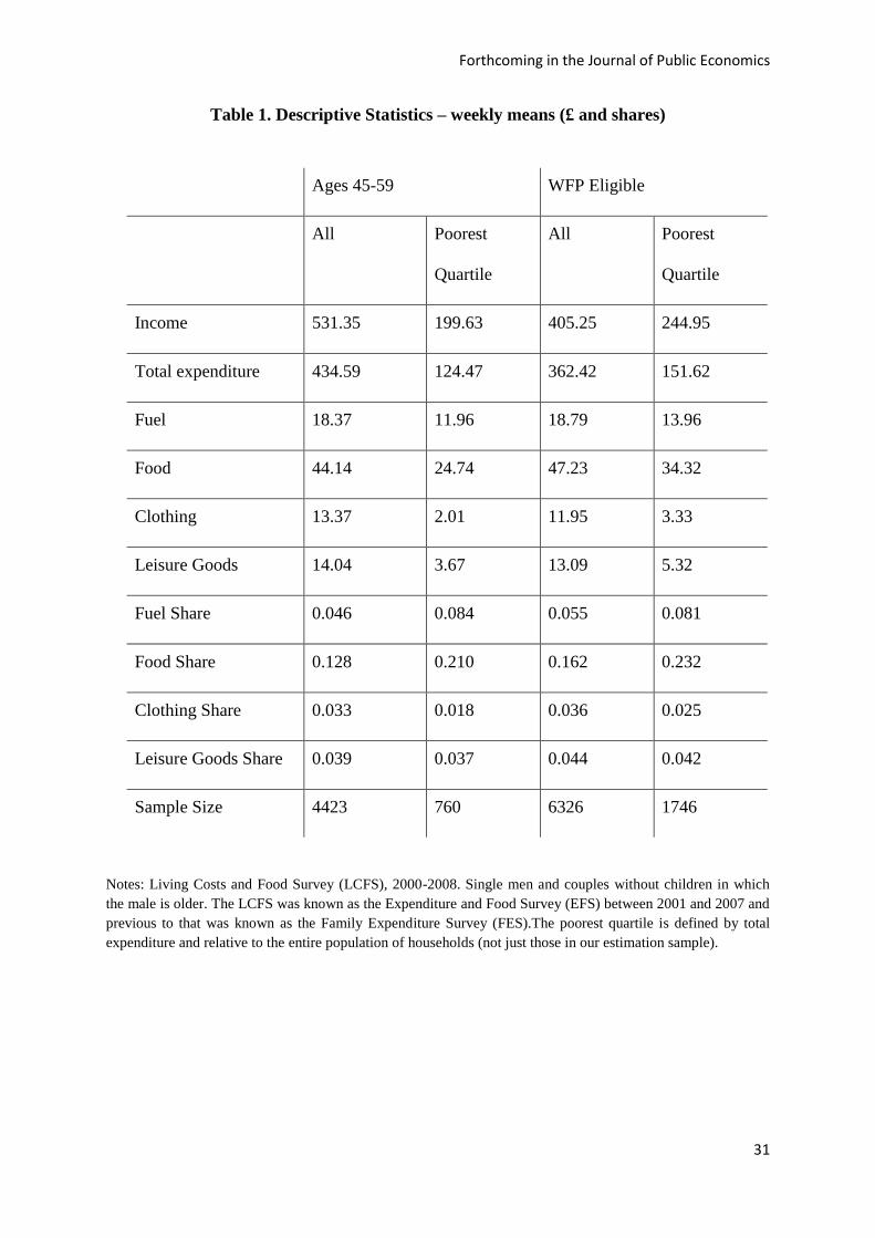
Table 1 presents summary statistics for our sample divided between eligible

households and households in which the oldest member is below the age cut-off. Eligible and


9

ineligible household differ in important ways. However, the regression discontinuity design

we describe below overcomes these differences by estimating an average treatment effect at

the eligibility threshold. That is, our research design rests not on the similarity of eligible and

ineligible households broadly, but on the similarity of those just above and below the

eligibility cut-off.

[TABLE 1 ABOUT HERE]

For both eligible and ineligible households, we present summary statistics for the

entire subsample, and for the poorest quartile of households as determined by household total

expenditure (we define quartiles with respect to the entire population of households and not

with respect to our estimation sample). Note that relative to the average, poorer households

spend less on fuel absolutely, but spend a larger share of their budget on fuel. Fuel is a

normal good, and a necessity. These facts are well known, but they play an important role in

our empirical design, which we turn to next.

3. Empirical Framework and Methods

Households where the eldest member turns 60 before the qualifying week are eligible

for the WFP and households where the eldest member turns 60 after the qualifying week are

not. This sharp eligibility criterion suggests estimating the effects of the WFP using a

regression discontinuity design (RDD). Take up of the WFP is very high (over 90%), and so a

research design based on the eligibility criterion can be considered a sharp RDD.

The intuition behind an RDD approach is straightforward: households immediately

below the cut-off provide evidence on how households immediately above the cut-off would

have behaved had they not received the transfer. The identifying assumption is that, in the

absence of the transfer, expenditures vary continuously with the forcing variable, age,

implying that, for the sample we consider, preferences and budget constraints evolve

smoothly with age. Any discrete change at age 60 is thus attributable to the average effect of


10

the WFP (at age 60).11

Age has previously been used as the forcing variable in regression

discontinuity designs. See for example: Edmonds et al. (2005), Card et al. (2008), Carpenter

and Dobkin (2009) and Lee and McCrary (2009).

3.1 Labeling Effects in an Engel Curve Framework

As noted above, if households do not adjust spending until an anticipated benefit is

received, receipt of WFP might lead to a change in fuel spending simply because of a

standard income effect. In our analysis we need to distinguish a labeling effect from an

income effect and to assess whether the WFP is allocated differently to how an unlabeled

transfer would be allocated. Therefore, we embed a regression discontinuity design within an

Engel curve framework. If households on either side of the eligibility criteria spend

significantly different shares of expenditure on fuel, holding total expenditure constant, this

would be direct evidence of a labeling effect.

In standard demand analysis, Engel curves measure the relationship between

household spending on a good and total household expenditure as total expenditure increases.

A common empirical specification of Engel curves relates budget shares to the logarithm of

total expenditure. Fuel is a normal good so as the level of total expenditure rises we would

expect fuel expenditure to rise. Because fuel is also a necessity, we would expect it to rise

less quickly than total expenditure, and so the budget share should fall. These are standard

income effects. Thus, an increase in fuel spending, or a decrease in the fuel budget share,

with receipt of the WFP might simply represent a standard move along the Engel curve – i.e.

an income effect; this is illustrated by the move from point A to point B in Figure I, where the

Engel curve is presented in share form. In contrast, if there is a labeling effect, when a

11

In principle we could also search for an effect at age 80, at which point the WFP becomes more

generous. However, in the LCFS age has been top-coded at 80 since 2002 which means that we are

unable to implement the RDD around age 80.


11

household receives a labeled transfer, they will shift off this Engel curve, as illustrated in

Figure 2 by the move from point B to point C.


To test for a labeling effect, while allowing for standard income effects, we estimate

standard Engel curves, which relate budget shares to a function of total expenditure,

combined with a regression discontinuity at age 60. We begin with a graphical analysis of

age-specific nonparametric Engel Curves. We then proceed to the RDD by estimating

parametric Engel curves augmented by the forcing variable (age) and other controls.

There are several advantages to working with the share form of Engel curves.

Extensive experience in modeling household demands has shown that working with shares

significantly reduces heteroscedasticity, and that budget shares are well modeled by a low-

order polynomial in the logarithm of total expenditure. In U.K. micro data the fuel share, in

particular, is approximately linear in the logarithm of total expenditure (see for example

Banks, Blundell and Lewbel, 1997). A further advantage is that an unmeasured increase in

income or other resources at age 60 would drive the share down (because fuel is a necessity)

and so bias our framework against finding a labeling effect. However, as a robustness check,

we also estimate our main model with fuel expenditures as the outcome variable of interest.

In our RDD estimates we allow preferences to evolve continuously with the forcing

variable, age of the oldest household member, Ai, by including polynomials in age (we use a

quadratic specification which minimizes Akaike’s Information Criterion and the Bayesian

Information Criterion). We augment this empirical specification with a dummy, Di, for WFP

eligibility. This variable captures any discontinuity in the way that budget shares vary with

age, conditional on total expenditure (and other covariates). We attribute any such

discontinuity to the effect of labeling the transfer. Eligibility is related to age by 1[𝐴𝑖 ≥ 60]

where 1[. ] is the indicator function. As per Lee and Lemieux (2010), we interact 60iA


12

and 2

60iA with program eligibility to allow the slope and curvature of the regression line

to differ on either side of the eligibility cut-off. Finally, we include a number of covariates,

Zi, to increase the precision of the regression discontinuity estimator and to capture variation

in relative prices. In all specifications, these include household size, month, area, and year. In

all specifications we also interact area dummies, and total expenditure variables (capturing

f (X) ) with year dummies. In several specifications we also include employment (of head

and, where relevant, spouse), housing tenure, number of rooms and education controls.

Hence, in complete form, our regression discontinuity Engel curve specification,

using quadratic terms in age, can be written:

wki

=a +tDi+ b

1Ai-60( ) + b

2Ai-60( )

2

+Di× b

3Ai-60( ) +D

i× b

4Ai-60( )

2

+dT × f Xi( ) +g TZ

i+ e

i (1)

where e is an independent (and possibly heteroscedastic) disturbance term and,

the

dependent variable is the budget share of good k, and

60 60lim [ | 60, , ] lim [ | 60, , ]k kA A

E w A Z z X x E w A Z z X x

provides a local estimate of the

effect of the WFP on budget shares at age 60, holding total expenditure constant. We estimate

this model (and all subsequent models except where otherwise stated) using least squares and

report robust standard errors.

This specification imposes that the labeling effect on the budget share, if any, is

independent of the level of total expenditure.12

We will test this specification below.13

In results presented below, we specify f (X) to be a quadratic function of the natural

logarithm of total expenditure, but results are robust to more flexible specifications. Note that

the total expenditure variables are also interacted with year dummies; within the constraints

12

Of course, this specification implies that the effect, in any, on pounds of fuel expenditure varies

with the level of total expenditure.

13 In Beatty et al. (2011) we lay out a more general specification that nests equation (1).


13

imposed by theory, we want to allow the form of the Engel curves we estimate to be quite

general and so we allow the slope (as well as the intercept) of the Engel curve to change as

relative prices change. This is important to ensure that the discontinuity effect we estimate is

not picking up changes in the shape of the Engel curve over time that we have not allowed

for.

We now turn to possible threats to the validity of this research design and how we

deal with them.

3.2 Measurement of Age

The LCF collects information on age in years at the time of interview but not date of

birth. If we assume that households where the oldest member of the household is 60 receive

the benefit then some misclassifications will occur. Recall that eligibility is determined

according to age in the ‘qualifying week’ – which during the period covered by our data was

in September. Consider then a household – interviewed, for example, on January 1st who

reports that the oldest member of the household is 60. If that person were born in January

through to the qualifying week in September of the previous year, they would be eligible for

the WFP, whereas if they were born after the qualify week (roughly October through to

January), they would not. Thus the probability that this household is eligible is about eight

twelfths. A household interviewed in February with the oldest member age 60 has a lower

probability of being eligible. A household interviewed in December with the oldest member

age 60 has a higher probability of being eligible. If birth dates and interview dates are

distributed evenly throughout the year, the average probability that a household with the

oldest member age 60 (at the interview date) is WFP eligible is one half. In our sample, the

distribution of interview dates (which we do observe) suggests a slightly higher probability of

about 52%, again assuming that birth dates (which we do not observe) are evenly distributed

through the year.


14

In spite of this, in what follows we classify households where the oldest member of

the household is 60 as receiving the WFP. If the benefit has a positive labeling effect on fuel

budget shares, our approach will bias downward the estimates of that effect (by

misclassifying some untreated households as treated) and so yield a conservative estimate. As

we are misclassifying approximately half of 60 year olds, the true effect for those of that age

will approach twice the impact that we find. There is no misclassification of eligibility among

households where the oldest member is 61 or older. We investigate the robustness of our

approach by re-estimating the labelling effect on a sample that omits households in which the

oldest individual reports an age of 60. This alternative strategy should not suffer from

attenuation bias, but it estimates the effect of the WFP on 61 year olds, rather than 60 year

olds.

3.3 Measurement Error in Total Expenditure

One possible concern is that measurement error in household expenditure could bias

our estimate of the effect of WFP. In general, measurement error in one variable can

potentially bias the estimate of all regression coefficients. In a simple example with classical

measurement error where the only regressors are log expenditure and WFP receipt, the bias

on the WFP coefficient would have the same sign as the relationship between log expenditure

and the fuel share, which is negative, and so the bias would actually be downwards (against

finding a labeling effect – this is, again, a benefit of working with the share form of Engel

curves). However, we cannot be sure that this would be the case in our more complicated

specification. Therefore, as a check, we follow standard practice in demand analysis and

instrument total expenditure with household income.

3.4 Employment Effects

From 1988 onwards individuals aged 60 or over have been entitled to a benefit, the

name and exact details of which have changed, but which is essentially a pensioner minimum


15

income guarantee (i.e. a minimum income guarantee without obligation to seek work). From

1988 to 1999 this was called Pensioner Income Support, from 1999 to 2003 it was known as

the Minimum Income Guarantee, and in 2003 this was replaced with Pension Credit. For the

rest of this paper we will refer to this benefit as the Minimum Income Guarantee (MIG).

Therefore, note that we do not have a period where age 60 brings only eligibility for WFP;

from 1988-1996 we have the MIG alone and from 1997-2008 we have the MIG plus WFP.14

Whilst we would not expect the MIG to have a labeling effect, it might have a labor

market participation effect, and, if consumption is not separable from leisure, this in turn will

have an effect on spending patterns. Specifically, when a working individual turns 60, they

become entitled to the MIG and they might prefer stopping work and receiving the MIG to

carrying on in employment. But dropping out of the labor market might influence spending

patterns; someone who is now at home for more of the day might heat their home more and

therefore have higher fuel spending. While the analysis in Blundell et al. (2011) indicates that

there is no evident discontinuity in male labor supply (at either the extensive or intensive

margin) at age 6015

, among our specification tests we include employment and self-

employment dummies and hours of work for both the head of household and (where there is

one) the spouse.

14 The means testing of housing and council tax benefit associated with the MIG became more

generous part way through our policy period, in 2003. Thus after 2003, turning 60 was associated with

somewhat larger transfers for some. However, we condition on total expenditure, which should

capture variation in resources, and, as argued above, additional resources that we fail to control for

should lead to lower, rather than higher fuel shares. Widespread travel discounts and free off-peak

travel in London significantly predate the introduction of WFP, but free off-peak travel outside

London was introduced in 2006. The substitution effect of a lower price of going out should be less

time at home (and hence perhaps lower fuel shares); the income effect should also lower the share of

necessities like fuel. 15

While there is a discontinuity in female labour supply at 60 (the age of eligibility for the state

pension for women), recall from Section 2 that we exclude from the sample single women and

couples where the woman is older. As a result no household in our sample first receives the state

pension and WFP at the same time – and our identification strategy is unaffected by discontinuities in

female labour supply at age 60.


16

It might be that controlling for observable labor market status in this way is enough to

deal with this (potential) issue. However, using 1988-1996 as a falsification test allows an

additional check on whether our results are contaminated by the labor market effect of the

MIG. Estimating an RDD on a pre-program period as a falsification test is normally good

practice (see, for example Lemieux and Milligan (2008)), but here it is particularly important

because the potential confounding of the WFP effect by the MIG. A significant effect in

these data would falsify the assumption that preferences evolve continuously with age.

3.5 Distinguishing Labeling from Intra-household Allocation

Effects

We noted above that in investigations of labeling and child benefit payments it is

difficult, in two-parent households, to distinguish a labeling effect from an effect induced by

the payment increasing the bargaining power of the woman. The WFP differs from child

benefit in that there is no compelling reason to believe that its effect on spending patterns

works through the intrahousehold distribution of income receipt. First, as noted above, there

is reason to think that the intrahousehold distribution of income receipt is particularly

important in the case of spending on children. In contrast, there is no obvious reason to think

that the intrahousehold distribution of income receipt is particularly important for spending

on fuel by older households. Second, in the sample of couples we have selected the male

member is always older. Thus at the eligibility threshold for WFP, only the male is eligible

and when only one member of a household is eligible for WFP, the transfer is paid to that

member. This means that, when implemented on our sample of couples in which the husband

is older, our regression discontinuity design studies the effect of a labeled transfer to

husbands. In the birth cohorts we study husbands were the primary earners and it is

implausible that this £250 transfer had a significant effect on the influence those husbands

had over household spending patterns. Finally, as a robustness check we implement our

analysis separately for singles and couples.


17

3.6 Additional Robustness Checks and Falsification Tests

Regression discontinuity designs can be sensitive to the choice of the range of the

forcing variable included in the regression, here the age of the oldest household member.

Our basic specification uses a window of fifteen years on either side of the discontinuity (45-

75). As a robustness check we re-estimate with a window of ten years on either side of the

discontinuity (50-70) and using the Imbens & Kalyanaraman (2012) optimal bandwidth in a

local linear regression discontinuity design framework.

We also repeat our analysis in levels of expenditure, rather than budget shares.

Although levels of expenditure are noisier, and more heteroscedastic than shares, this

provides a direct estimated of the impact on fuel spending.

Finally, we conduct a further falsification test. We rerun our main analysis but with

cut-offs at 55 and 65 rather than 60. Under the maintained assumptions of the regression

discontinuity design we should not find discontinuities (in levels or shares) at these age cut-

offs.

4. Results

4.1 Graphical Evidence

As suggested by Lee and Lemieux (2010), we begin with a straightforward graphical

presentation. Figure 3 plots the average fuel expenditure share in one-year age bins, over the

range 45-75, with a locally-weighted regression line overlaid on either side of the eligibility

threshold for the WFP. The top panel uses data from 2000 to 2008, when the WFP was in

effect. The bottom panel uses data from 1988 to 1996, prior to the introduction of the WFP.

The fuel share appears to change smoothly over time, with a fairly clear jump of roughly one

percentage point at age 60 in the period during which the WFP was paid. This jump is not

evident in the earlier period.

[FIGURES 3 ABOUT HERE]


18

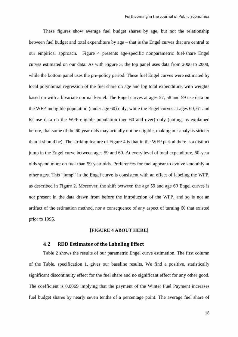
These figures show average fuel budget shares by age, but not the relationship

between fuel budget and total expenditure by age – that is the Engel curves that are central to

our empirical approach. Figure 4 presents age-specific nonparametric fuel-share Engel

curves estimated on our data. As with Figure 3, the top panel uses data from 2000 to 2008,

while the bottom panel uses the pre-policy period. These fuel Engel curves were estimated by

local polynomial regression of the fuel share on age and log total expenditure, with weights

based on with a bivariate normal kernel. The Engel curves at ages 57, 58 and 59 use data on

the WFP-ineligible population (under age 60) only, while the Engel curves at ages 60, 61 and

62 use data on the WFP-eligible population (age 60 and over) only (noting, as explained

before, that some of the 60 year olds may actually not be eligible, making our analysis stricter

than it should be). The striking feature of Figure 4 is that in the WFP period there is a distinct

jump in the Engel curve between ages 59 and 60. At every level of total expenditure, 60-year

olds spend more on fuel than 59 year olds. Preferences for fuel appear to evolve smoothly at

other ages. This “jump” in the Engel curve is consistent with an effect of labeling the WFP,

as described in Figure 2. Moreover, the shift between the age 59 and age 60 Engel curves is

not present in the data drawn from before the introduction of the WFP, and so is not an

artifact of the estimation method, nor a consequence of any aspect of turning 60 that existed

prior to 1996.


4.2 RDD Estimates of the Labeling Effect

Table 2 shows the results of our parametric Engel curve estimation. The first column

of the Table, specification 1, gives our baseline results. We find a positive, statistically

significant discontinuity effect for the fuel share and no significant effect for any other good.

The coefficient is 0.0069 implying that the payment of the Winter Fuel Payment increases

fuel budget shares by nearly seven tenths of a percentage point. The average fuel share of


19

those aged 45 to 59 is 4.6 percent, so this is substantial increase in spending on fuel. We

interpret this effect on the fuel share, holding total expenditure constant, as a labeling effect.16

Recall that this estimate understates the full effect for those aged 60 because our approach

misclassifies some of those who do not receive the benefit as receiving it (those who have

reached age 60 at when surveyed but had not done so at the preceding eligibility cutoff date).

We find no statistically significant effects on the share spent on food, clothing and

leisure goods.17

We also report estimates for total expenditure. While total expenditure is

lower for eligibles than for non-eligibles (see Table 1) there is no evidence of a discontinuity

at age 60. This affirms that the changes in shares reported in the rows above reflect changes

in the pattern of expenditures.

In column (2) we add additional control variables for education, employment, housing

tenure and number of rooms in the home. The positive effect on the fuel share is robust to the

inclusion of these additional controls. In column (3) we instrument for total expenditure with

household income to account for the possibility of measurement error in total expenditure.18

This has almost no impact on the estimated labeling effect. Although our quadratic age

polynomial used in each of these three specifications was chosen to minimize Akaike’s

Information Criterion, we experimented with higher order polynomials and found that our

16

The standard errors reported in the linear regressions here are robust to heteroskadasticity. We have

also examined the results obtained using one-way clustering on both age and year. In both cases, we

find smaller standard errors on the coefficient indicating the discontinuity. In presenting the results

therefore, we have, conservatively, chosen the standard errors that result in the least likelihood of

finding significant results. We have also tested the results obtained using two-way clustering on age

and year using the method suggested by Cameron et al. (2011). The variance covariance matrix in this

case is not of full rank. In such a situation Cameron et al. (2011) suggest setting the negative

eigenvalues of that matrix to zero. When we proceed in this manner, the statistically significant effect

of the winter fuel payment on fuel budget share remains.

17 Of course, the budget constraint implies that the positive effect on fuel spending must be offset by

reductions elsewhere, though the offset could be spread over many goods and hence difficult to detect. 18 To illustrate the strength of the instrument we have estimated regressions of the logarithm of

total expenditure on the logarithm of current income year by year. The smallest t-statistic we

find on income is 12.05 and smallest coefficient on log income (the elasticity) is 0.36.


20

results were entirely robust to variations in the specification of the age variables. These

results are not reported in the table but are available on request.

These regressions control for the total level of expenditure. The coefficient for the

base year on total expenditure in these regressions lies between -0.032 and -0.035 (these are

not reported in the tables). That the fuel share falls with total expenditure confirms that well

known fact that fuel spending is a necessity, as noted above.

Column (4) of Table 2 shows the results from the implementation of the local linear

regression discontinuity estimator and applies the optimal bandwidth of Imbens &

Kalyanaraman (2012).19

In each case the optimal bandwidth is close to 1 year. Identification

here, then, comes from comparing households located immediately on each side of the

threshold. Applying this estimator yields a larger point estimate than that found using our

baseline specification.


Table 3 shows the results of four additional robustness checks. Column (1) takes the

baseline specification augmented with additional controls and narrows the age window to 10

years on either side of age 60. Column (2) implements the local linear regression

discontinuity design estimator with double the optimal bandwidth (i.e. uses a bandwidth of 2

years). The estimated effect on fuel budget share of WFP receipt in each of these cases is

positive, significant and of a similar magnitude to our baseline estimate. Column (3) drops

those aged 60 – some of whom will be classified as having received the WFP when they have

not, - so that the comparison is between 59 and 61 year olds. In this case the coefficient falls

slightly, despite the fact that this comparison does not suffer from the attenuation effect

arising from the misclassification of 60 year olds. This suggests that the labelling effect of the

WFP is strongest when first received, and then diminishes. In fact, this pattern is also

19

This is estimated using the Stata package of Nichols (2012).


21

apparent in Figure 3. In the pre-policy period, the fuel budget share rises gently with age

(bottom panel). The Winter Fuel Payment appears to bring forward and accelerate this shift in

spending (top panel).

The fourth column of Table 3 reports the results from a regression of the levels of fuel

expenditure rather than shares. The estimate here is also positive and statistically significant.

The point estimate indicates that the payment of the WFP (of £250) induces additional

expenditure of over £75 annually on fuel.


Table 4 presents the results of our falsification tests. In Column (1) we report

estimates of a discontinuity at age 60 in the period before the WFP was introduced (1988-

1996)20

. This is effectively an omnibus test of many possible mis-specifications that might

affect the validity of our research design. If the positive effects of eligibility on fuel spending

documented in Table 2 are driven by any misspecification or omitted factor that pre-dated the

introduction of the policy, we should find evidence of that here. In particular, if the results are

driven by differences in labor-supply (and consequent differences in household technology)

then we should find an effect in this 1988-1996 falsification period in which the incentives

for a retirement around age 60 (including the MIG) were broadly the same.

As column (1) of Table 4 reports, we find no discontinuity in fuel spending at age 60

in the 1988-1996 pre-policy period. In fact, the coefficient on the age 60 dummy is negative,

although it is not statistically different from zero.

20

In an earlier version of the paper we report the results of estimating a “differenced-RDD”

specification on pooled data from 1988-1996 and 2000-2008. This is therefore the average effect of

the WFP on budget shares at age 60, conditional on total expenditure and net of any employment

effect at age 60. The point estimate for this “differenced-RDD” specification was larger than our

estimates in Table II. This is because, as we see in our falsification test (Table IV), in the placebo

period (1988 to 1986) the estimated coefficient on the eligibility dummy (age 60 and above) is

negative (though not statistically different from zero.) The differenced-RDD estimate is less precisely

estimated than the estimates in Table II, but is still significant at the 5% level. Full details are

available on request.


22

Columns (2) and (3) of Table 5 report tests for discontinuities in the relationship

between age and fuel budget share at ages 55 and 65, five years before and after eligibility for

the WFP. Note that the latter (age 65) is the focal retirement age in the UK. As with the pre-

policy period, we find no effect. Thus we are unable to find any evidence that contradicts the

assumptions of RDD design.


Our basic specification imposes that the labeling effect on budget shares, if present, is

unrelated to the level of total expenditure and to any other variable. In Table 5 we report the

results of relaxing this assumption and allowing the effect to vary by quartile of total

expenditure, by season, and by household type. Mostly the coefficients are not precisely

estimated, which is to be expected given the now much smaller sample sizes. We can only

marginally reject at the 10% level the hypothesis that there are no differences between

expenditure quartiles – with a larger effect for poorer households, and we cannot reject nulls

of no differences between groups defined by season and household types. In interpreting the

absence of any significant difference between the seasons, it should be kept in mind that over

half of all households pay for their fuel using equal installment plan (see Beatty et al. (2014)

for more details) and so additional consumption of fuel in winter will therefore result in

increased spending on fuel throughout the year.21

We discussed in Section 3 the reasons for which we think it implausible that the

results we find come from an intrahousehold effect rather than from a labeling effect. Despite

these considerations discussed there, it is reassuring to see, in column (3), that the labeling

21 As noted above some 60 year olds are mis-classified as treated when they are not. This will vary by

season and so it is possible that our estimates of effects by season are biased by this. However, we

have re-estimated these interactions dropping the 60 year olds (following the robustness check in

Column (3) of Table 3. When we do so, we are still unable to reject a common effect across all

seasons.


23

effect is still significant when we split our sample into single men and couples. This confirms

that the effect we find is indeed a labeling effect and not, instead, an intra-household effect.

The point estimate for single men is larger than for couples (although, as stated, not

significantly different from each other) but, again, the average total expenditure of this

sample of single men is much lower than the couples sample.


To summarize, we find a positive effect of WFP eligibility on the budget share of

fuel, conditional on total expenditure and allowing preferences to evolve with age in a

continuous fashion. The effect is strongly statistically significant and robust across alternative

specifications. Because of the very high take-up of this transfer among eligible households,

the effect of eligibility is for all intents and purposes also the effect of receipt. We attribute

this effect to the labeling of this transfer. A series of falsification tests failed to contradict our

identifying assumptions, and in particular, we find no evidence of a confounding of the

labeling effect with employment effects around age 60.

5 DISCUSSION

5.1 Price Effects

One further threat to our analysis is the idea that over-60 households pay lower prices for

fuel. Note that given the results of our falsification tests, it would have to be the case that this

was only true after 1996. There is no government policy of lower fuel prices for seniors of

which we are aware. It is true that various charitable service organizations provide advice to

seniors on how to find the best energy tariffs, and it is possible that such organizations are

more active in recent years than previously. However, empirical estimates show that fuel

demands are price inelastic (again see Banks, Blundell and Lewbel, 1997 as an example).

This means that lower prices would lead to lower, rather than higher, fuel shares.

5.2 Reporting Effects


24

Our spending data are from surveys, raising the possibility that receipt of the winter

fuel payments changes reports of fuel spending rather than fuel spending itself. However, as

noted above, most of the fuel spending information comes from the questionnaire which is

completed with the interviewer present, and respondents are asked to consult bills and report

the value of their last payment. Thus an effect on reporting behavior is unlikely.

5.3 Magnitudes

We can translate the magnitudes in Table 2 into spending changes as follows.

Ignoring other covariates for simplicity, if

𝑤𝑘 =𝑥𝑘

𝑋= 𝑓(𝑥)

then

𝜕𝑥𝑘

𝜕𝑋=

𝜕𝑤𝑘

𝜕𝑋𝑋 + 𝑤𝑘

so if households receive a transfer of 𝑤𝑓𝑝 then the slide along the Engel curve starting from

total budget 𝑋 (the move from A to B in Figure 1) is approximately

(𝜕𝑤𝑘

𝜕𝑋𝑋 + 𝑤𝑘) 𝑤𝑓𝑝

and if our estimate of the movement off the Engel curve measured in percentage points of

budget share (the move from B to C in Figure 1) is 𝜏, then the estimate of the labeling effect

measured in pounds of expenditure is approximately.

𝜏(𝑋 + 𝑤𝑓𝑝) (2)

With the results from, say, specification 2 in Table 2 our estimate of the slide along

the Engel curve for someone with the average fuel share in 2008 of 0.0613 and total budget

of around £308 per week receiving a transfer of £250 a year (so just under £5 a week) is

£0.128 with a standard error of 0.010 and a 95% confidence interval around this point

estimate of £0.108 to £0.148. Our estimate of the labeling effect is £2.13 with a standard error

of 0.592 and 95% confidence interval of £0.97 to £3.29. In other words, if there was no


25

labeling effect an average household would spend around 3% of a small transfer on fuel. We

estimate an additional labeling effect of 44% (with a confidence interval of 20% to 68%) so

that the overall marginal propensity to spend on fuel associated with the WFP is around 47%.

Again note that is a conservative estimate of the effect for those aged 60 (because household

members who are 60 at the interview date, but did not turn 60 before the eligibility cutoff

result in some mis-measurement of eligibility), and that, on the other hand, the data suggest

the effect is largest at age 60.

Equation (2) shows that the absolute labeling effect depends on the estimated size of

the discontinuity and on total household expenditure. Therefore, the different shifts estimated

by expenditure quartile translate into point estimates of additional labeling effects of £2.81,

£1.73, £0.91 and £1.38 respectively.

6 Conclusion

This paper asks whether labeling an unconditional cash transfer has any effect on the

way in which recipients spend it. In other words, does calling the £250 that most elderly

households in the UK receive in November / December a “Winter Fuel” payment make any

difference? Sharp differences in the eligibility requirements allow us to use a regression

discontinuity design to examine how fuel expenditure changes on receipt of the benefit. We

find a substantial and robust labeling effect. Our estimate of the (average) marginal

propensity to spend on household fuel out of unlabeled income is approximately 3%. On

average, we find recipient households exhibit an additional marginal propensity to spend on

household fuel out of the WFP of between about 20% and 68%, and so the combined effect is

between 23% and 71%. The data also suggest that the labelling effect of the WFP is strongest

when first received, and then diminishes.

The direct interpretation of this is straightforward: if households are given an

unconditional and neutrally-named cash transfer of £100 they would be expected to spend


26

approximately £3 on household fuel. If they are given an unconditional cash transfer called

the Winter Fuel Payment in the middle of winter we estimate that they will spend between

£23 and £71 on fuel (our point estimate is £47). Overall, our evidence implies that the label

of this particular transfer has a critical impact on the behavioral response of those who

receive it.

Labeling effects have been reported for child benefits but are not robustly replicated

in different countries and, where they have been found, are not robustly distinguished from an

intrahousehold effect. The other large transfer program with labeling that has been

extensively studied is food stamps (in the U.S). The best quasi-experimental studies of food

stamps do not find any framing or labeling effect; infra-marginal consumers treat food stamps

as a cash transfer, as standard economic theory would predict. Thus our findings are at odds

with most of the existing literature. Our findings are for a large labeled transfer that has not

been studied before and are based on a different identification strategy (the regression design)

than the prior literature. We also go beyond those papers that have found labeling effects in

an important way by robustly ruling out an intrahousehold effect as an explanation for the

differential spending of the transfer.

An unresolved challenge is to understand the mechanism behind this large effect. As

noted in the introduction, a possibility is that it is a result of mental accounting, though it is

unclear why such a mechanism would operate for WFP in the U.K. but not for food stamps in

the U.S. An alternative explanation is that elderly people in the U.K. take the labeling of the

WFP as health advice, about the importance of staying warm, from a credible source (the

government). Food stamps might not be interpreted in the same way. This is cannot a full

explanation as governments offer a wide range of health advice to their populations, some of

which is followed and some of which is ignored. Resolving the detailed mechanism at work


27

when a government labels transfers will require further research, with greater variation in

details of the labeling and in the contexts in which it occurs.


28

References

Abler, Johannes and Marklien, Felix, 2010. “Fungability, Labels and Consumption.”

University of Nottingham, Working Paper.

Banks, James, Blundell, Richard and Arthur Lewbel, 1997. “Quadratic Engel Curves and

Consumer Demand’’ The Review of Economics and Statistics, vol. 79(4), pages 527-

Beatty, Tim .K., Laura Blow and Thomas F. Crossley, 2014. “Is there a ‘heat-or-eat’ trade-off

in the UK?” Journal of the Royal Statistical Society: Series A, vol. 177(1), pages 281-

294.

Beatty, Tim .K., Laura Blow, Thomas .F. Crossley and C. O’Dea, 2011. “Cash By Any Other

Name? Evidence on Labeling From the UK Winter Fuel Payment.” Institute for Fiscal

Studies WP 11/10.

Blow, Laura, Ian Walker and Yu Zhu, 2010, “Who Benefits from Child Benefit?”, Economic

Inquiry, vol. 50(1), pages 153-170.

Blundell, Richard, Antoine Bozio, and Guy Laroque. 2011. “Labour Supply and the Intensive

Margin.", American Economic Review, vol. 11(3), p. 482-86.

Brewer, M., Muriel, A., Phillips, D. and Sibieta, L. (2008), Poverty and Inequality in the UK:

2008, Commentary no. 105, London: Institute for Fiscal Studies.

Cameron, A. Colin, Jonah B. Gelbach, and Douglas, L. Miller, 2011. "Robust Inference With

Multiway Clustering," Journal of Business & Economic Statistics, vol. 29(2), pages

238-249.

Card, David, Dobkin Carlos and Maestas, Nicole, 2008. “The Impact of Nearly Universal

Insurance Coverage on Health Care: Evidence from Medicare,” American Economic

Review, vol. 98(5), pages 2242–58.


29

Card, David, and Ransom, Michael, 2011. “Pension plan characteristics and framing effects

in employee savings behavior,” The Review of Economics and Statistics, 93(1), pages

228-243.

Carpenter, Christopher & Dobkin, Carlos, 2009. “The Effect of Alcohol Consumption on

Mortality: Regression Discontinuity Evidence from the Minimum Drinking Age,”

American Economic Journal: Applied Economics, vol. 1(1), pages 164-182.

Edmonds, Eric, 2002."Reconsidering the labeling effect for child benefits: evidence from a

transition economy," Economics Letters, Elsevier, vol. 76(3), pages 303-309.

Edmonds, Eric V., K Mammen and D. Miller, 2005. “Rearranging the Family? Household

Composition Responses to Large Pension Receipts,” The Journal of Human

Resources, vol. 40(1), pages 186-207.

Hines, James R., and Thaler, Richard H., 1995, “Anomalies: The Flypaper Effect”, Journal of

Economics Perspectives, vol. 9(4), pages 217-226, Fall.

Hoynes, Hilary, and Diane Whitmore Schanzenbach (2009), “Consumption Responses to the

In-Kind Transfers: Evidence from the Introduction of the Food Stamp Program”.

American Economic Journal: Applied Economics, 1:4,109-139.

Imbens, Guido, and Kalyanaraman, 2012. “Optimal Bandwidth Choice for the Regression

Discontinuity Estimator,” Review of Economic Studies, 79:3, 933-959.

Kooreman, Peter, 2000."The Labeling Effect of a Child Benefit System," American

Economic Review, vol. 90(3), pages 571-583.

Lee, David S. and Card, David, 2008, “Regression Discontinuity with Specification Error,”

Journal of Econometrics, vol. 142(2), pages 655-674.

Lee, David S. and Lemieux, Thomas, 2010. “Regression Discontinuity Designs in

Economics,” Journal of Economic Literature. vol. 48(2) , pages 281-355.


30

Lee, David S. and McCrary, Justin, 2009. “The Deterrence Effect of Prison: Dynamic Theory

and Evidence”, Working Paper 550, Princeton University, Department of Economics,

Industrial Relations Section.

Lemieux, Thomas and Milligan, Kevin, 2008. “Incentive effects of social assistance: A

regression discontinuity approach,” Journal of Econometrics, vol. 142(2) pages 807-

828.

Matheson, Jil, 1991. “Application of Computer Assisted Interviewing to the Family

Expenditure Survey,” Office of National Statistics.

http://www.ons.gov.uk/ons/guide-method/method-quality/survey-methodology-

bulletin/smb-29/survey-methodology-bulletin-29.pdf

Moffitt, Robert, 1989. "Estimating the Value of an In-Kind Transfer: The Case of Food

Stamps," Econometrica, vol. 57(2), pages 385-409.

Nichols, Austin. 2011. rd 2.0: Revised Stata module for regression discontinuity estimation.

http://ideas.repec.org/c/boc/bocode/s456888.html

Parker, John A., Nicholas S. Souleles, David S. Johnson & Robert McClelland, 2013.

"Consumer Spending and the Economic Stimulus Payments of 2008," American

Economic Review, vol. 103(6), p. 2530-53.

Thaler, Richard and Sunstein, Cass 2008. Nudge: Improving Decisions About Health,

Wealth, and Happiness. New Haven, CT: Yale University Press.

Thaler, Richard H., 1990. “Saving, fungibility and mental accounts”, Journal of Economic

Perspectives, vol. 4(1), pages 193-205.

Thaler, Richard H., 1999. “Mental accounting matters”, Journal of Behavioral Decision

Making, vol. 12(3), pages 183–206.

Zantomio, Francesca, 2008. “The Route to Take-up: Raising Incentives or Lowering

Barriers?” Mimeo, Institute for Social and Economic Research, University of Essex.


31

Table 1. Descriptive Statistics – weekly means (£ and shares)

Ages 45-59 WFP Eligible

All Poorest

Quartile

All Poorest

Quartile

Income 531.35 199.63 405.25 244.95

Total expenditure 434.59 124.47 362.42 151.62

Fuel 18.37 11.96 18.79 13.96

Food 44.14 24.74 47.23 34.32

Clothing 13.37 2.01 11.95 3.33

Leisure Goods 14.04 3.67 13.09 5.32

Fuel Share 0.046 0.084 0.055 0.081

Food Share 0.128 0.210 0.162 0.232

Clothing Share 0.033 0.018 0.036 0.025

Leisure Goods Share 0.039 0.037 0.044 0.042

Sample Size 4423 760 6326 1746

Notes: Living Costs and Food Survey (LCFS), 2000-2008. Single men and couples without children in which

the male is older. The LCFS was known as the Expenditure and Food Survey (EFS) between 2001 and 2007 and

previous to that was known as the Family Expenditure Survey (FES).The poorest quartile is defined by total

expenditure and relative to the entire population of households (not just those in our estimation sample).


32

Table 2. RDD estimates.

Effects of WFP on budget shares

(conditional on total expenditure) and on total expenditure

Shares (1)

OLS

(2)

OLS

(3)

IV

(4)

Local linear

Fuel 0.0069*** 0.0068*** 0.0067*** 0.0083**

(0.0019) (0.0019) (0.0019) (0.0026)

Food 0.0007 0.0006 0.0008 0.0025

(0.0036) (0.0036) (0.0036) (0.0045)

Clothing -0.0008 -0.0011 -0.0011 -0.0052

(0.0030) (0.0030) (0.0030) (0.0043)

Leisure Goods 0.0014 0.0011 0.0012 0.0020

(0.0029) (0.0028) (0.0029) (0.0037)

Total expenditure 0.0170 0.0098 --------- 0.0265

(0.0321) (0.0279) (0.0346)

Age Window 45-75 45-75 45-75 59-60 (Optimal)

Number of observations 10,749 10,749 10,749 854

Data Period 2000-

2008

2000-

2008

2000-

2008

2000-2008

Additional Controls Y Y Y

Notes:

1. The base specification for the share regressions contains the following controls: (the natural logarithm of)

total expenditure and its square; year dummies, region dummies and their interactions; interactions between

the year dummies and the total expenditure variables; month dummies; and (the natural logarithm of)

household size. The additional controls are employment, self-employment and hours (of the head, and where

relevant, the spouse), housing tenure, number of rooms and education controls. The results on total

expenditure include the same controls (with the exception of total expenditure itself).

2. The age window pertains to the oldest person in the household.

3. Robust standard errors are given in parentheses


33

4. † = significant at 10% level, * = significant at 5% level, ** = significant at 1% level, *** = significant at

0.1% level

Table 3. Robustness Checks

(1)

OLS

(2)

Local linear

(3)

OLS

(4)

OLS

Dependent Variable Budget

Share

Budget

Share

Budget

Share

Expenditure

Level

Effect of WFP on

Annual Fuel Spending

0.0079*** 0.0094** 0.0060**

(0.0021)

75.44*

(0.0023) (0.0039) (36.44)

Age Window 50-70 2*Opt. 45-75 45-75

Data Period 2000-2008 2000-2008 2000-2008 2000-2008

Number of observations 7,985 1,722 10,338 10,749

Additional Controls Y Y Y Y

Robustness Check Smaller age

window

Twice

optimal bw

(Ages 58-

61)

Dropping

age 60

Levels

Notes:

1. The base specification includes the following controls: (the natural logarithm of) total expenditure and its

square; year dummies, region dummies and their interactions; interactions between the year dummies and the

total expenditure variables; month dummies; and (the natural logarithm of) household size. The additional

controls are employment, self-employment and hours (of the head, and where relevant, the spouse), housing

tenure, number of rooms and education controls.


3. Robust standard errors are given in parentheses.


0.1% level


34

Table 4. Falsification Tests

Effects on Fuel Budget Share

(Conditional on Total Expenditure)

Shares (1)

OLS

(2)

OLS

(3)

OLS

Prior to Policy

Introduction

Discontinuity at

55

Discontinuity at

65

Fuel -0.0018 0.0027 -0.0014

(0.0021) (0.0025) (0.0019)

Age Window 45-75 45-756 45-75

6

Number of observations 10,614 10,749 10,749

Data Period 1988-1996 2000-2008 2000-2008

Additional Controls Y Y Y

Notes:

1. The base specification includes the following controls: (the natural logarithm of) total expenditure

and its square; year dummies, region dummies and their interactions; interactions between the year

dummies and the total expenditure variables; month dummies; and (the natural logarithm of)

household size. The additional controls are employment, self-employment and hours (of the head,

and where relevant, the spouse), housing tenure, number of rooms and education controls.



4. † = significant at 10% level, * = significant at 5% level, ** = significant at 1% level, *** =

significant at 0.1% level

5. Rebalancing the sample (for example changing the age window around 55 to be 40-70) also yields

insignificant results.


35

Table 5. RDD estimates for different sub-groups

Effects of WFP on budget Shares

(conditional on total expenditure)

(1)

Expenditure Quartile:

(2)

Season:

(3)

Household Type:

1st 0.0205** Winter 0.0085† Single man 0.0105*

(0.0077) (0.0044) (0.0048)

2nd

0.0066† Spring 0.0074† Couple 0.0048**

(0.0035) (0.0038) (0.0019)

3rd

0.0022 Summer 0.0083*

(0.0025) (0.0035)

4th

0.0019 Autumn 0.0042

(0.0021) (0.0036)

F-test

(p-value)

F(3,10129) = 2.16

(0.09)

F(3,10165) = 0.29

(0.83)

F(1,10433)= 1.23

(0.27)

Age Window 45-75 45-75 45-75

No. obs. 10,749 10,749 10,749

Data Period 2000-2008 2000-2008 2000-2008

Add. Conts. Y Y Y

Notes:

1. The base specification includes the following controls: (the natural logarithm of) total expenditure and its

square; year dummies, region dummies and their interactions; interactions between the year dummies and the

total expenditure variables; month dummies; and (the natural logarithm of) household size. The additional

controls are employment, self-employment and hours (of the head, and where relevant, the spouse), housing

tenure, number of rooms and education controls.




0.1% level


36

Figure 1: Sample size by age

0

50

100

150

200

250

300

350

400

450

500

45

46

47

48

49

50

51

52

53

54

55

56

57

58

59

60

61

62

63

64

65

66

67

68

69

70

71

72

73

74

75

Sam

ple

siz

e

Age


37

Figure 2: Engel Curve with

Income Effect and Labeling Effect


38

Figure 3: Fuel budget shares by age

(a) 2000 – 2008 Winter Fuel Payment in Effect

(b) 1988 – 1996 Pre- Policy Period

3.0%

3.5%

4.0%

4.5%

5.0%

5.5%

6.0%

6.5%

7.0%

45

46

47

48

49

50

51

52

53

54

55

56

57

58

59

60

61

62

63

64

65

66

67

68

69

70

71

72

73

74

75

Fue

l bu

dge

t sh

are

Age

3.0%

4.0%

5.0%

6.0%

7.0%

8.0%

9.0%

10.0%

45

46

47

48

49

50

51

52

53

54

55

56

57

58

59

60

61

62

63

64

65

66

67

68

69

70

71

72

73

74

75

Fue

l bu

dge

t sh

are

Age


39

Figure 4: Fuel Engel Curves by Age

(a) 2000 – 2008 Winter Fuel Payment in Effect

(b) 1988 – 1996 Pre- Policy Period

Notes: Fuel Engel curves estimated by local polynomial regression of the fuel share on age and log total

expenditure, with weights based on with a bivariate normal kernel (with age and log total expenditure as

arguments). This allows the fuel share to vary in a general way with age and log total expenditure. The Engel

curves at ages 57, 58 and 59 use data on the WFP-ineligible population (under age 60) only, while the Engel

curves at ages 60, 61 and 62 use data on the WFP-eligible population (over age 60 and over) only.

.03

.04

.05

.06

.07

.08

fuel sh

are

-1 -.5 0 .5 1standardised log expenditure

age_57 age_60

age_58 age_61

age_59 age_62

.04

.06

.08

.1.1

2

fuel sh

are

-1 -.5 0 .5 1standardised log expenditure

age_57 age_60

age_58 age_61

age_59 age_62

cash by any other name? evidence on labeling from …repository.essex.ac.uk/12155/1/wfp jpube...

Documents