case study 1: estimating click probabilities · 2013-01-10 · 1 1 l2 regularization for logistic...

1

1

L2 Regularization for Logistic Regression

Machine Learning/Statistics for Big Data CSE599C1/STAT592, University of Washington

Carlos Guestrin January 10th, 2013

©Carlos Guestrin 2013

Case Study 1: Estimating Click Probabilities

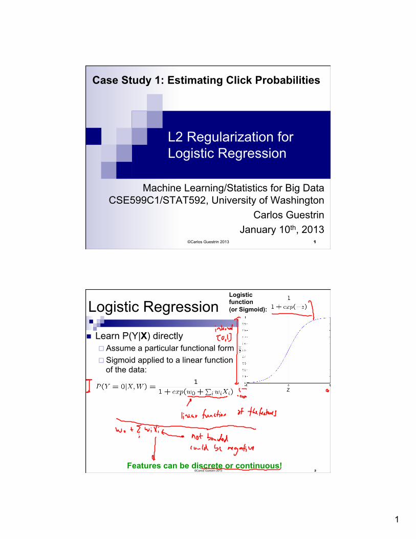
Logistic Regression Logistic function (or Sigmoid):

n  Learn P(Y|X) directly ¨ Assume a particular functional form ¨ Sigmoid applied to a linear function

of the data:

Z

Features can be discrete or continuous! 2 ©Carlos Guestrin 2013

2

Optimizing concave function – Gradient ascent

n  Conditional likelihood for Logistic Regression is concave. Find optimum with gradient ascent

n  Gradient ascent is simplest of optimization approaches ¨  e.g., Conjugate gradient ascent much better (see reading)

Gradient:

Step size, η>0

Update rule:

3 ©Carlos Guestrin 2013

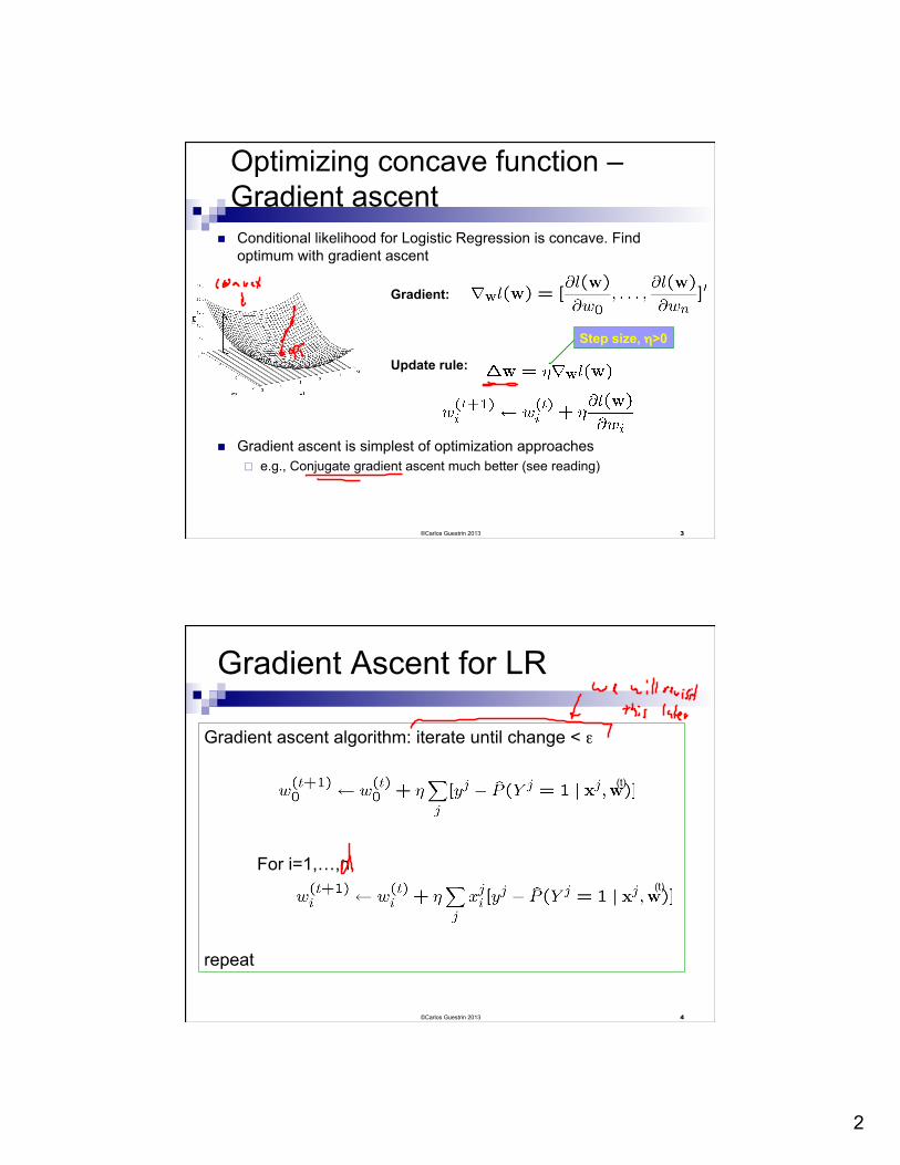
Gradient Ascent for LR

Gradient ascent algorithm: iterate until change < ε

For i=1,…,n,

repeat


(t)

(t)

3

Test set error as a function of model complexity


Regularization in linear regression

n  Overfitting usually leads to very large parameter choices, e.g.:

n  Regularized least-squares (a.k.a. ridge regression), for λ>0:

-2.2 + 3.1 X – 0.30 X2 -1.1 + 4,700,910.7 X – 8,585,638.4 X2 + …


4

©Carlos Guestrin 2013 7

Linear Separability

8

Large parameters → Overfitting

n  If data is linearly separable, weights go to infinity n  Leads to overfitting:

n  Penalizing high weights can prevent overfitting… ©Carlos Guestrin 2013

5

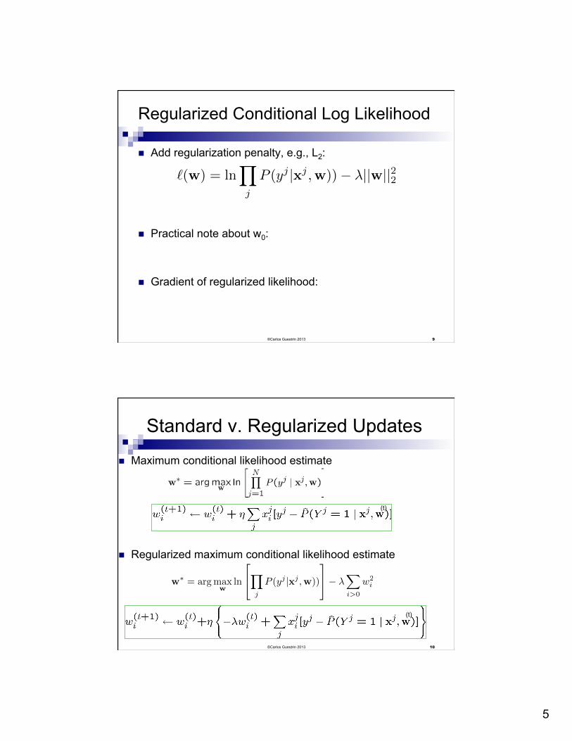
Regularized Conditional Log Likelihood

n  Add regularization penalty, e.g., L2:

n  Practical note about w0:

n  Gradient of regularized likelihood:


`(w) = lnY

j

P (yj |xj ,w))� �||w||22

10

Standard v. Regularized Updates

n  Maximum conditional likelihood estimate

n  Regularized maximum conditional likelihood estimate


(t)

(t)

w

⇤= argmax

wln

2

4Y

j

P (yj |xj ,w))

3

5� �X

i>0

w2i

6

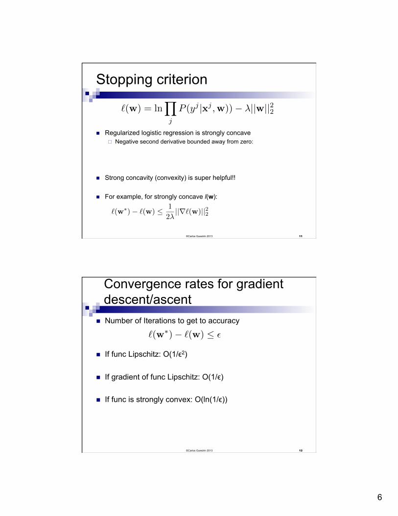
Stopping criterion

n  Regularized logistic regression is strongly concave ¨  Negative second derivative bounded away from zero:

n  Strong concavity (convexity) is super helpful!!

n  For example, for strongly concave l(w):


`(w) = lnY

j

P (yj |xj ,w))� �||w||22

`(w⇤)� `(w) 1

2�||r`(w)||22

Convergence rates for gradient descent/ascent

n  Number of Iterations to get to accuracy

n  If func Lipschitz: O(1/ϵ2)

n  If gradient of func Lipschitz: O(1/ϵ)

n  If func is strongly convex: O(ln(1/ϵ))


`(w⇤)� `(w) ✏

7

What you should know about Logistic Regression (LR) and Click Prediction

n  Click prediction problem: ¨  Estimate probability of clicking ¨  Can be modeled as logistic regression

n  Logistic regression model: Linear model n  Optimize conditional likelihood n  Gradient computation n  Overfitting n  Regularization n  Regularized optimization n  Convergence rates and stopping criterion


14

Online Learning Perceptron Algorithm Kernels

Machine Learning/Statistics for Big Data CSE599C1/STAT592, University of Washington

Carlos Guestrin January 10th, 2013


Case Study 1: Estimating Click Probabilities

8

Challenge 1: Complexity of Computing Gradients


(t)

Challenge 2: Data is streaming

n  Assumption thus far: Batch data

n  But, click prediction is a streaming data task: ¨  User enters query, and ad must be selected:

n  Observe xj, and must predict yj

¨  User either clicks or doesn’t click on ad: n  Label yj is revealed afterwards

¨  Google gets a reward if user clicks on ad

¨  Weights must be updated for next time:


9

Online Learning Problem

n  At each time step t: ¨  Observe features of data point:

n  Note: many assumptions are possible, e.g., data is iid, data is adversarially chosen… details beyond scope of course

¨  Make a prediction: n  Note: many models are possible, we focus on linear models n  For simplicity, use vector notation

¨  Observe true label: n  Note: other observation models are possible, e.g., we don’t observe the label directly, but only a noisy version... Details

beyond scope of course

¨  Update model:


The Perceptron Algorithm [Rosenblatt ‘58, ‘62] n  Classification setting: y in {-1,+1} n  Linear model

¨  Prediction:

n  Training: ¨  Initialize weight vector: ¨  At each time step:

n  Observe features: n  Make prediction: n  Observe true class:

n  Update model: ¨  If prediction is not equal to truth


10

Mistake Bounds

n  Algorithm “pays” every time it makes a mistake:

n  How many mistakes is it going to make?



Linear Separability: More formally, Using Margin

n  Data linearly separable, if there exists ¨ a vector ¨ a margin

n  Such that

11

Perceptron Analysis: Linearly Separable Case

n  Theorem [Block, Novikoff]: ¨  Given a sequence of labeled examples:

¨  Each feature vector has bounded norm:

¨  If dataset is linearly separable:

n  Then the number of mistakes made by the online perceptron on this sequence is bounded by


Perceptron Proof for Linearly Separable case

n  Every time we make a mistake, we get gamma closer to w*: ¨  Mistake at time t: w(t+1) = w(t) + y(t) x(t) ¨  Taking dot product with w*: ¨  Thus after k mistakes:

n  Similarly, norm of w(t+1) doesn’t grow too fast: ¨ 

¨  Thus, after k mistakes:

n  Putting all together:


||w(t+1)||2 = ||w(t)||2 + 2y(t)(w(t) · x(t)) + ||x(t)||2

12

Beyond Linearly Separable Case n  Perceptron algorithm is super cool!

¨  No assumption about data distribution! n  Could be generated by an oblivious adversary,

no need to be iid ¨  Makes a fixed number of mistakes, and it’s

done for ever! n  Even if you see infinite data

¨  Constant cost per iteration n  Converges in O(1/ϵ)

n  However, real world not linearly separable ¨  Can’t expect never to make mistakes again ¨  Analysis extends to non-linearly separable

case ¨  Very similar bound, see Freund & Schapire

from Readings ¨  Converges, but ultimately may not give good

accuracy (make many many many mistakes)



What if the data is not linearly separable?

Use features of features of features of features….

Feature space can get really large really quickly!

13


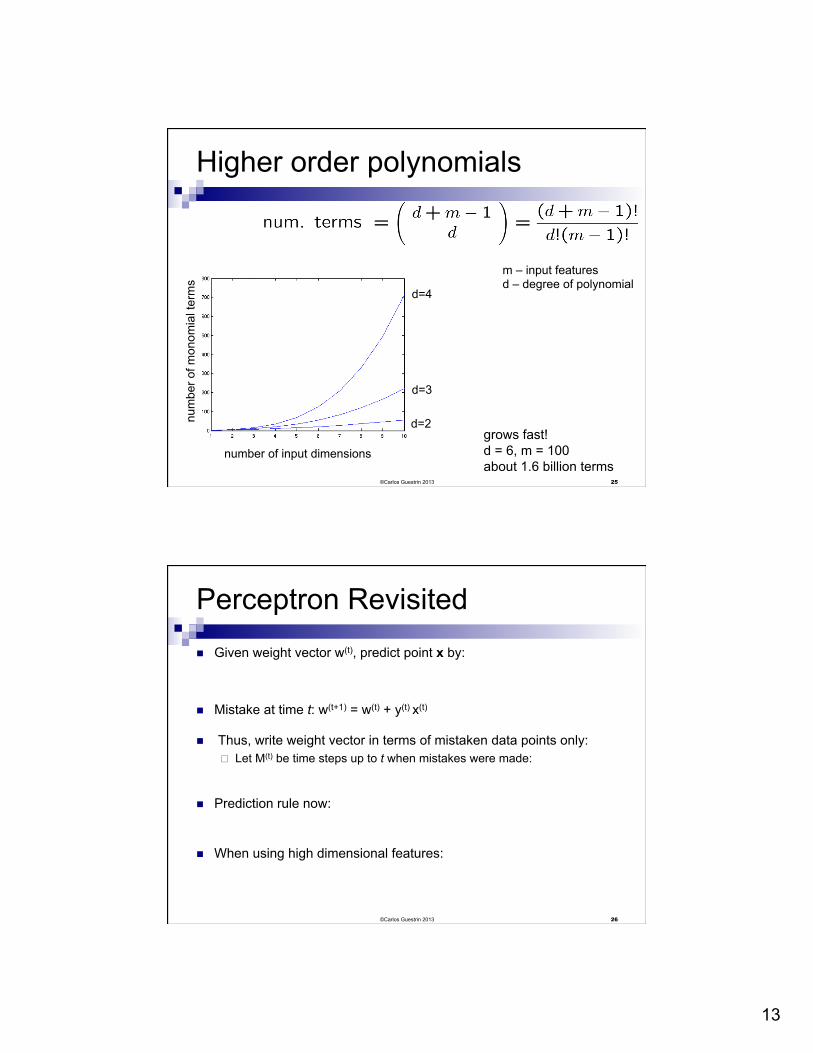
Higher order polynomials

number of input dimensions

num

ber o

f mon

omia

l ter

ms

d=2

d=4

d=3

m – input features d – degree of polynomial

grows fast! d = 6, m = 100 about 1.6 billion terms

Perceptron Revisited n  Given weight vector w(t), predict point x by:

n  Mistake at time t: w(t+1) = w(t) + y(t) x(t)

n  Thus, write weight vector in terms of mistaken data points only: ¨  Let M(t) be time steps up to t when mistakes were made:

n  Prediction rule now:

n  When using high dimensional features:


14


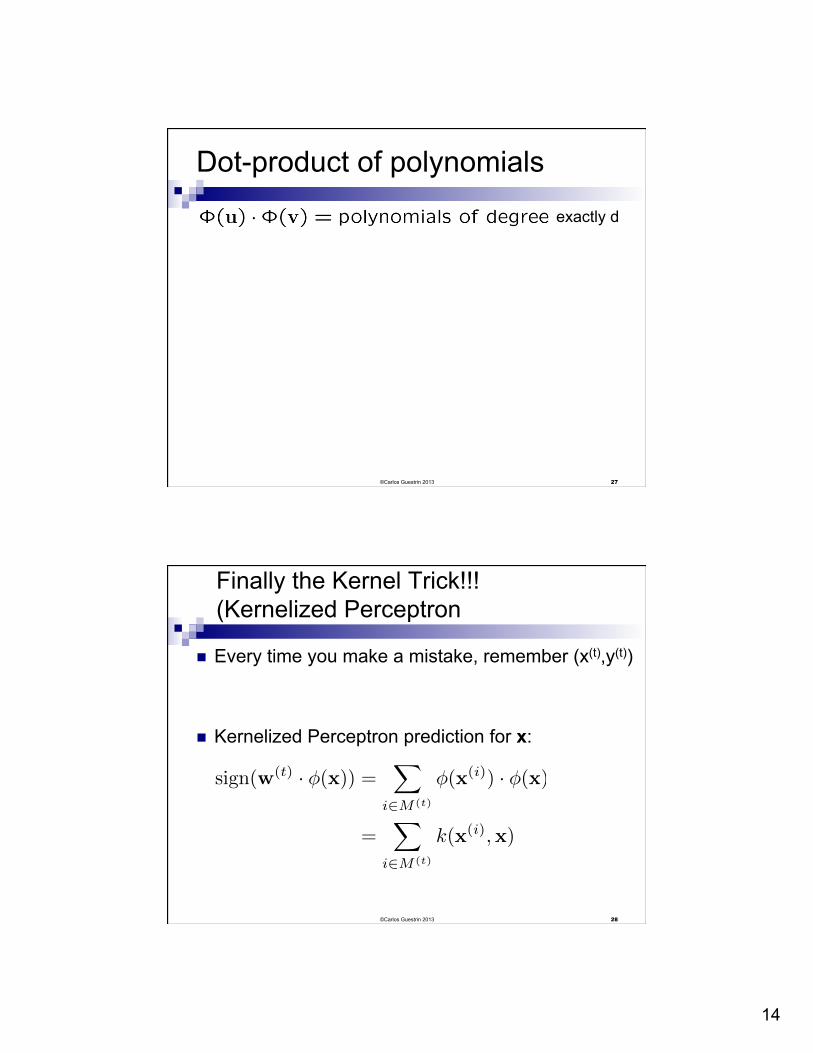
Dot-product of polynomials

exactly d

Finally the Kernel Trick!!! (Kernelized Perceptron

n  Every time you make a mistake, remember (x(t),y(t))

n  Kernelized Perceptron prediction for x:


sign(w(t) · �(x)) =X

i2M(t)

�(x(i)) · �(x)

=X

i2M(t)

k(x(i),x)

15


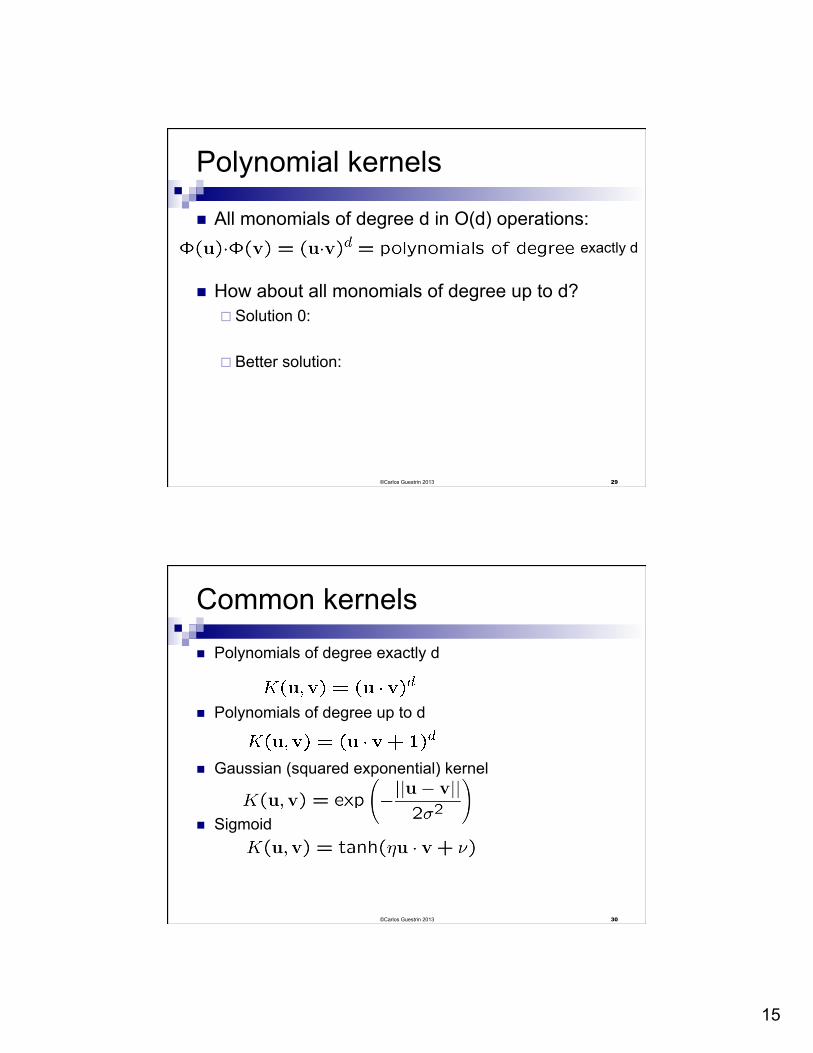
Polynomial kernels

n  All monomials of degree d in O(d) operations:

n  How about all monomials of degree up to d? ¨ Solution 0:

¨ Better solution:

exactly d


Common kernels

n  Polynomials of degree exactly d

n  Polynomials of degree up to d

n  Gaussian (squared exponential) kernel

n  Sigmoid

16

Fundamental Practical Problem for All Online Learning Methods: Which weight vector to report?

n  Suppose you run online learning method and want to sell your learned weight vector… Which one do you sell???

n  Last one?

n 

n 

n 


Choice can make a huge difference!!


[Freund & Schapire ’99]

17


What you need to know

n  Notion of online learning n  Perceptron algorithm n  Mistake bounds and proofs n  The kernel trick n  Kernelized Perceptron n  Derive polynomial kernel n  Common kernels n  In online learning, report averaged weights at the end

case study 1: estimating click probabilities · 2013-01-10 · 1 1 l2 regularization for logistic...

Documents