case fil copy - nasa · mately 1000 (octal) words. ... nbro number of trajectories already...

NASA TECHNICAL

MEMORANDUM

CMw»CO

NASA TM X-3529

CASE FILCOPY

THREE-DIMENSIONAL RANDOM EARTH ATMOSPHERES

FOR MONTE CARLO TRAJECTORY ANALYSES

Janet W. Campbell

Langley Research Center

Hampton, Va. 23665

NATIONAL AERONAUTICS AND SPACE ADMINISTRATION • WASHINGTON D. C. • AUGUST 1977

https://ntrs.nasa.gov/search.jsp?R=19770023097 2018-07-17T06:55:27+00:00Z

1. Report No. 2. Government Accession No. 3. Recipient's Catalog No.

NASA TM X-35294. Title and Subtitle

THREE-DIMENSIONAL RANDOM EARTH ATMOSPHERESMONTE CARLO TRAJECTORY ANALYSES

7. Author(s)

Janet W. Campbell

9. Performing Organization Name and AddressNASA Langley Research CenterHampton, VA 23665

12. Sponsoring Agency Name and AddressNational Aeronautics and Space AdministratWashington, DC 205^6

5. Report DateFOR August 1977

6. Performing Organization Code

8. Performing Organization Report No.

L-1062310. Work Unit No.

506-26-30-08

11. Contract or Grant No.

13. Type of Report and Period CoveredTechnical Memorandum

ion14. Sponsoring Agency Code

15. Supplementary Notes

16. Abstract

A set of four computer tapes containing random three-dimensional Earth atmo-spheres is available for Monte Carlo trajectory analyses. The four tapes - one foreach season - contain sufficient atmospheric tables to allow over 1400 replicationsof any trajectory below an altitude of 99 km. The atmospheres were provided by anempirical model designed to generate random atmospheres whose distributions matchthose in a data base of over 6000 sounding-rocket measurements. A readily imple-mentable means of linking the tapes to any existing trajectory simulation computerprogram is. described. It involves the addition of three subroutines which arelisted in an appendix.

17. Key Words (Suggested by Author(s))

Three-dimensional atmosphereRandom atmospheresMonte CarloTrajectory simulation

/•

19. Security Qassif. (of this report) 20. Security Classif. (of this

Unclassified Unclassified

18. Distribution Statement

Unclassified - Unlimited

Subject Category 88

page) 21. No. of Pages 22. Price*

45 $4.00

* For sale by (he National Technical Information Service, Springfield. Virginia 22161

THREE-DIMENSIONAL RANDOM EARTH ATMOSPHERES FOR

MONTE CARLO TRAJECTORY ANALYSES

Janet W. CampbellLangley Research Center

SUMMARY

A set of four magnetic computer tapes containing random global Earth atmo-spheres is available for Monte Carlo trajectory analyses below an altitude of99 km. The four tapes - each representing a different season - contain atmo-spheres in sufficient quantity to permit over 1400 independent replications ofany trajectory.

The atmospheres were generated by a statistical atmosphere model based onover 6000 rocket and high-altitude soundings. The model was constructed empiri-cally to generate temperatures, densities, and pressures whose distributionsmatch those in the data, and whose vertical gradients are likewise statisticallysimilar to gradients in the data.

A readily implementable means of interfacing the tapes with an existingtrajectory simulation program is described. The method involves the additionof three subroutines, which are linked to the trajectory "program through simplecalling statements. The core storage required for the subroutines is approxi-mately 1000 (octal) words.

INTRODUCTION

There is a recognized need among aircraft and spacecraft designers for ameans of estimating the impact of atmospheric variability on a vehicle's perform-ance. Standard Atmospheres (refs. 1 to 3) are commonly used to calculate trajec-tories, but the Earth's atmosphere is variable and always differs from any stan-dard. For example, high-altitude densities at a fixed location can vary by over100 percent within the same season. Densities vary by at least 10 percent atall altitudes.

The Random Earth Atmosphere Computer Tapes (REACT) are a set of four mag-netic tapes containing typical nonstandard densities and temperatures for athree-dimensional global atmosphere. The tapes are intended to be used alongwith a trajectory simulation program to generate samples of trajectories passingthrough different random atmospheres. Such samples can help define the variabil-ity in a vehicle's performance parameters resulting from atmospheric variations.Any vehicle (spacecraft or aircraft) can be studied by using the tapes in theflight regime where the altitude is below 99 kilometers.

The REACT atmospheres are profiles of temperatures and densities generatedby the empirical random atmosphere (ERA) statistical model (ref. 4) which was

developed empirically from over 6000 meteorological rocket and high-altitudesoundings. Pressure and other atmospheric properties (e.g., viscosity, speed ofsound, etc.) can be calculated from the temperatures and densities. The atmo-spheres on the tapes are described as typical in that their statistical distri-butions match those of the sounding data at corresponding altitudes, latitudes,and seasons.

The tapes represent four seasons as follows:

Tape

12

. 34

Months

March to MayJune to August

September to NovemberDecember to February

Tape identification

SPRINGSUMMERAUTUMNWINTER

(The season designation refers to that of the northern hemisphere. For example,the."SPRING" tape actually contains autumn atmospheres for southern hemispherelocations.)

Each tape contains sufficient atmospheric data to permit up to 361 indepen-dent replications of the same trajectory, the actual number depending on therange of longitudes covered by .that trajectory. The trajectory's performanceparameters (for example, range, surface heating rates, dynamic pressures, struc-tural loads, etc.), which are of interest to the vehicle designer, will varyfrom one replication to the next because of the atmosphere's variability. Thecollection of parameter values resulting from the simulations forms a randomstatistical sample which can be used to estimate that parameter's underlyingprobability distribution. Such distributions are needed in estimating the prob-ability of exceeding existing design values, in establishing new design values,and in designing adequate guidance and control systems. Sources of error otherthan the atmosphere can be incorporated and a thorough error analysis performed.

Because the three-dimensional REACT atmospheres introduce certain densitygradient effects which are not provided by the standard atmospheric models, adiscussion of horizontal and vertical density gradients is included. Densitygradients on the tapes are compared with those in the data and with proposed"design" gradients in reference 5. Vertical density gradients are consistentwith those found in the data. Since the data base consists of isolated verticalprofiles, inferences about horizontal density gradients cannot be made directlyfrom the data. Horizontal gradients were controlled by assuming a minimum dis-tance between uncorrelated profiles of 600 nautical miles (ref. 6). A fairlyhigh percentage of the REACT density gradients exceeded the "design" gradientsof reference 5, even though the latter were based on this same assumption. Itis believed, however, that the REACT density gradients are more representativeof realistic gradients.

Three subroutines which can be used to link REACT to a trajectory programare described and a listing of the subroutines is given in appendix A. Appen-

dix B presents a brief description of the empirical atmosphere model (ref.used to generate the tapes.

SYMBOLS AND ABBREVIATIONS

ATMOS one of three subroutines used to interface REACT with trajectoryprogram

COMMON/LINK/ common storage area containing block information from TAPE10shared by ATMOS, INITBLK, and READBLK subroutines

D atmospheric density,

DL increment used to convert longitude to "longitude" on TAPE10, deg

g acceleration due to gravity, m/sec^

INITBLK one of three subroutines used to interface REACT with trajectoryprogram

k refers to a season in northern hemisphere; k = 1 (spring), k = 2(summer), k = 3 (autumn), and k = 4 (winter)

N in subroutine READBLK, refers to next block to be read from TAPE10

NBR simulation or replication number

NBRO number of trajectories already simulated from TAPE10 on previous runof program

NMAX maximum number of independent trajectories which can be simulated byusing TAPE10

NO number of TAPE10 block currently stored in COMMON/LINK/

P atmospheric pressure, N/m^

Pg2 1962 Standard Atmosphere pressure, N/m^

R gas constant used in equation of state, 8314.34 J-kmol~^-K~^

REACT Random Earth Atmosphere Computer Tapes

READBLK one of three subroutines used to interface REACT with trajectoryprogram

RHO three-dimensional array containing random atmospheric densities fromTAPE10, kg/m3

S speed of sound, m/sec

SEASON alphanumeric word used to identify REACT tape (first record on eachtape)

s standard deviation of atmospheric temperature estimated from soundingdata, K

T atmospheric temperature, K

f mean atmospheric temperature estimated from sounding data, K

TAPE 10 REACT tape linked to a trajectory program at any given time

TAU three-dimensional array containing random atmospheric temperaturesfrom TAPE10, K

W mean molecular weight of air, 28.964 kg-kmol~^

XLAT latitude, deg

XLATI initial latitude of trajectory, deg

XLATO latitude locating RHO and TAU arrays, deg

XLOMAX maximum longitude of trajectory, deg

XLOMIN minimum longitude of trajectory, deg

XLONG "longitude" on TAPE10, deg

XLONGI initial longitude of trajectory, deg

XLONGO "longitude" locating RHO and TAU arrays, deg

Z altitude, m

z altitude, km

X longitude, deg

p atmospheric density, kg/m^

P62 1962 Standard Atmosphere density, kg/m^

<t> latitude, deg

TAPE SPECIFICATIONS

The tapes are 1.27-cm (0.5-in.) nine-track magnetic tapes written in binary(odd parity) mode, using a density of 629.9 characters per cm (1600 characters perin.), and labeled with ANSI standard labels. They were generated on a CONTROLDATA CYBER 175 computer which uses a physical record size of 512 60-bit words.

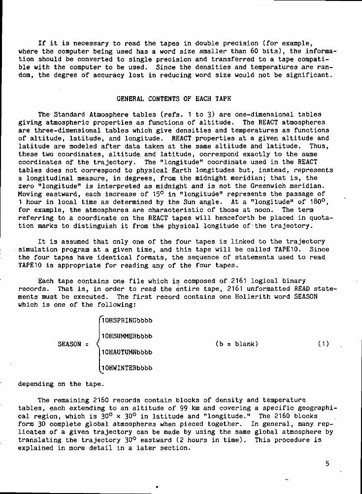
If it is necessary to read the tapes in double precision (for example,where the computer being used has a word size smaller than 60 bits), the informa-tion should be converted to single precision and transferred to a tape compati-ble with the computer to be used. Since the densities and temperatures are ran-dom, the degree of accuracy lost in reducing word size would not be significant.

GENERAL CONTENTS OF EACH TAPE

The Standard Atmosphere tables (refs. 1 to 3) are one-dimensional tablesgiving atmospheric properties as functions of altitude. The REACT atmospheresare three-dimensional tables which give densities and temperatures as functionsof altitude, latitude, and longitude. REACT properties at a given altitude andlatitude are modeled after data taken at the same altitude and latitude. Thus,these two coordinates, altitude, and latitude, correspond exactly to the samecoordinates of the trajectory. The "longitude" coordinate used in the REACTtables does not correspond to physical Earth longitudes but, instead, representsa longitudinal measure, in degrees, from the midnight meridian; that is, thezero "longitude" is interpreted as midnight and is not the Greenwich meridian.Moving eastward, each increase of 15° in "longitude" represents the passage of1 hour in local time as determined by the Sun angle. At a "longitude" of 180°,for example, the atmospheres are characteristic of those at noon. The termreferring to a coordinate on the REACT tapes will henceforth be placed in quota-tion marks to distinguish it from the physical longitude of-the trajectory.

It is assumed that only one of the four tapes is linked to the trajectorysimulation program at a given time, and this tape will be called TAPE10. Sincethe four tapes have identical formats, the sequence of statements used to readTAPE10 is appropriate for reading any of the four tapes.

Each tape contains one file which is composed of 2161 logical binaryrecords. That is, in order to read the entire tape, 2161 unformatted READ state-ments must be executed. The first record contains one Hollerith word SEASONwhich is one of the following:

SEASON = <

TOHSPRINGbbbb

lOHSUMMERbbbb(b = blank) (1)

lOHAUTUMNbbbb

lOHWINTERbbbbv.

depending on the tape.

The remaining 2160 records contain blocks of density and temperaturetables, each extending to an altitude of 99 km and covering a specific geographi-cal region, which is 30° x 30° in latitude and "longitude." The 2160 blocksform 30 complete global atmospheres when pieced together. In general, many rep-licates of a given trajectory can be made by using the same global atmosphere bytranslating the trajectory 30° eastward (2 hours in time). This procedure isexplained in more detail in a later section.

Each of the blocks must be read with a statement of the form

READ (10) NO,XLATO,XLONGO,RHO,TAU

where NO is the block number (NO = 1, . . ., 2160); XLATO and XLONGO are a ref-erence latitude and longitude which locate the block geographically; and RHO isan array of densities and TAU is an array of temperatures, both dimensioned34 x 4 x 4. The elements RHO(I,J,K) and TAU(I,J,K) are, respectively, atmo-spheric density, in kg/m3, and atmospheric temperature, in K, at

Altitude, km: z = 3(1 - 1) ( 1 = 1 , . . . ,

Latitude, deg: <|> = XLATO + 10(J - 1) (J = 1, . . ., 4)\ (2)

"Longitude," deg: X = XLONGO + 10(K - 1) (K = 1, . . ., 4)

Within each array the values are located every 3 km in altitude and every 10° inlatitude and "longitude." From the dimensions of the RHO and TAU arrays, it fol-lows that these tables cover the three-dimensional volume defined by

0 z z £ 99 km ^|

XLATO g <|> g XLATO + 30° \ (3)

XLONGO ^ X g XLONGO + -30°J

Figure 1 shows how the 2160 blocks fit together to cover the "longitude"-latitude plane. The number appearing in each block indicates the block numberNO. The reference point (XLONGO,XLATO) for a block is the grid point in thelower left-hand corner of that block. Blocks were stored on the tapes beginningat XLATO = -90° and XLONGO = 0°, and proceeding northward, keeping XLONGOfixed and increasing XLATO in increments of 30° until XLATO = 60°. Then XLONGOis increased by 30° and the same six values of XLATO are repeated. As theblocks encompass the Earth 30 times, the value of XLONGO goes from 0° to 10 770°(= 30 x 360° - 30°). It was more expedient from a programing standpoint toallow XLONGO to increase monotonically rather than set it back to 0° after eachrevolution. Near the equator the blocks cover an area approximately 3300 km by3200 km and near the poles they cover an area approximately 3300 km by 860 km.

The computer core storage required to read each block is 1091 words orslightly more than 2000 octal words. It should only be necessary to read andstore one block at a time. As the trajectory enters the three-dimensionalregion associated with a particular block, a subroutine should be called toread the appropriate block from TAPE10. The trajectory simulation can then con-tinue through this region until a boundary is reached. As the trajectory passesinto a new region, the subroutine should be called again to read the next appro-priate set of RHO and TAU values.

REPLICATION OF TRAJECTORIES

It is assumed that the user will want to maximize the number of independentreplicates of a trajectory which can be simulated by using TAPE10. That is, theuser will have a specific trajectory, such as a space shuttle entry trajectory,and will want to replicate this trajectory as many times as possible by usingdifferent random atmospheres from TAPE10.

Figure 2 shows the ground track of an entry trajectory from a 28.5°inclined orbit. The initial longitude and latitude, when z = 99 km, are -175°and -5°, respectively, and the final longitude and latitude are -119° and 36°,respectively. Figure 3 shows a set of independent replicates of this trajectoryrelative to the atmospheres on TAPE10. Notice that the first trajectory beginsat a "longitude" of 0°. The second begins at 30°, the third at 60°, and soforth. In simulating trajectories using different atmospheres from TAPE10, rep-licates will be independent provided that no two simulations use the same ele-ment of a RHO or TAU array to compute atmospheric properties. A 30° translationin "longitude" should result in trajectory replicates which are essentially inde-pendent. If ground tracks for different replicates approach or intersect oneanother when plotted on a latitude-"longitude" plane such as that in figure 3,the two replicates are not strictly independent. However, if their altitudes atpoints of intersection are substantially different, the dependence should beweak and can be ignored.

Since "longitudes" on TAPE10 actually represent time lines, the first tra-jectory in figure 3 starts at midnight, the second at 2 a.m., the third atk a.m., and so forth. If a large sample of replicates is generated or if thenumber of replicates is a multiple of 12, then the effect of local time willaverage out.

INCORPORATING REACT INTO A TRAJECTORY SIMULATION PROGRAM

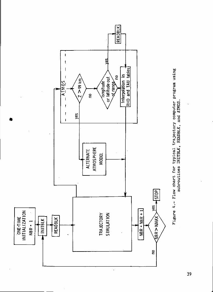
In order to interface a trajectory program with REACT, it is suggested thatthree subroutines, such as those listed in appendix A, be added. A flow chartutilizing these subroutines is shown in figure *J. The first INITBLK is calledonce at the beginning of each trajectory simulation to initialize the block. Itdetermines the trajectory's initial latitude and "longitude" relative to theblocks on TAPE10, and then calls the second subroutine READBLK which reads thecorrect block of information from TAPE10.

A third subroutine ATMOS is called at each point along a trajectory when-ever atmospheric properties (i.e., density, temperature, pressure, and speed ofsound) are needed. Presumably, ATMOS will replace any atmospheric model alreadyin the trajectory program and, as it will be called frequently, it should be asefficient as possible. ATMOS interpolates in the RHO and TAU arrays to give anatmospheric density and temperature at the altitude, latitude, and longitudespecified in its calling statement. Atmospheric pressure is then obtained fromthe equation of state, and the speed of sound is calculated from the temperature.(See formulation of ATMOS.) Before interpolating, a test is made to determinewhether the trajectory's altitude, longitude, and latitude are still within therange covered by the block currently stored. If it is outside the longitude-

latitude range, ATMOS calls READBLK to locate and read the correct block. Ifthe altitude is above 99 km, ATMOS calls an alternate atmosphere model which theuser must supply. In most instances it is sufficient to let this be the nonran-dom atmosphere previously used to calculate trajectories.

The subroutines are written so as to be readily incorporated into an exist-ing trajectory program. The only link between the trajectory program and thesubroutines is through the calling statements to the subroutines INITBLK andATMOS whose arguments are in terms of true longitudes. Conversion to "longi-tudes" relative to the coordinates on TAPE10 is handled automatically by thesubroutines. Replication of trajectories is also handled automatically in thatINITBLK calculates the initial "longitude" of each successive replicate, trans-lating it 30° eastward from its previous initial "longitude." A more detaileddescription of the formulation of each subroutine follows.

SUBROUTINE INITBLK - FORMULATION

INITBLK must be called once prior to each replication of a trajectory. Thebasic purpose of INITBLK is to initialize the COMMON storage area

COMMON/LINK/ DL.NO.XLATO.XLONGO.RHOGM,1*) ,TAU(3M,4)

which is shared by all three subroutines. (See appendix A.) During a simula-tion, NO, XLATO, XLONGO, RHO, and TAU will contain the most recent block ofinformation read from TAPE10, and DL is an increment used to convert longitudesto "longitudes" on TAPE10 by the translation

"Longitude" = Longitude + DL (4)

The calling statement for INITBLK is

CALL INITBLK (NBR, NMAX, XLATI, XLONGI, XLOMIN, XLOMAX)

where NBR = 1, 2, 3, • • • is the number of the replication about to be simu-lated; NMAX is an output variable which gives the maximum number of independentreplications which can be simulated using TAPE10; XLATI and XLONGI are the ini-tial latitude and longitude, respectively, of the trajectory; and XLOMIN andXLOMAX are the minimum and maximum longitudes, respectively, of the trajectory.All arguments except NBR should remain constant throughout the simulations.

The first time INITBLK is called, the calling program must set NBR = 1.At this time, DL is initialized so that the minimum longitude XLOMIN correspondsto a "longitude" on TAPE10 of 0.001°. (This value is effectively zero but asmall positive increment is used to prevent a negative zero "longitude" fromoccurring because of machine round-off error.) Thus, the increment DL is calcu-lated as

DL = 0.001 - XLOMIN (5)

The initial longitude XLONGI becomes the "longitude"

XLONG = XLONGI + DL (6)

on TAPE10, and the maximum number of independent replicates is calculated as

NMAX = HO 80° - XLOMAX - DL] + 1 (7)L 30 J

where here and in later formulas the brackets indicate the "greatest integer"function defined by

^greatest integer £ x if x £ 0M = ' (8)

( smallest integer ^ x if x < 0

INITBLK then sets NO = 0 and calls READBLK to read the block covering the point(XLATI, XLONG), where XLONG is defined in equation (6).

On subsequent calls to INITBLK, NBR must be greater than 1. At this timeDL is increased by 30° and the new XLONG is calculated by equation (6). Aftereach replication is simulated and before calling INITBLK for the next replica-tion, NBR should be tested to make sure it does not exceed NMAX.

As an example, consider the trajectory shown in figure 2. The first callto INITBLK would be

CALL INITBLKd,NMAX,-5.0,-175.0,-175.0,-119.0)

When INITBLK returns control to the calling program, the value of NMAX will be359 and will remain constant throughout the run. Thus, a sample of 359 indepen-dent replications of this trajectory can be generated from each tape or 1H36 rep-lications by using all four tapes. Of course, the user can always make fewerreplications.

As another example, figure 5 shows the groundtrack of an entry trajectoryfrom a 10^o inclined orbit. The first call to-INITBLK for this trajectory wouldbe

CALL INITBLKd,NMAX,73-0,4.0,-123.0,1.0)

Note that the minimum longitude (-123°) is neither the initial nor the final lon-gitude in this case. Here INITBLK returns with NMAX = 356, and the possiblereplications are illustrated in figure 6.

SUBROUTINE READBLK - FORMULATION

READBLK is called both from INITBLK, to initialize RHO and TAU at the begin-ning of each trajectory replication, and from ATMOS whenever the trajectoryenters a region requiring new RHO and TAU arrays. The calling statement toREADBLK is

CALL READBLK(XLAT,XLONG)

where -90° < XLAT $ 90° and 0° 1 XLONG $ 10 800° are the present latitudeand "longitude" relative to the blocks on TAPE10.

At the time READBLK is called, NO is the number of the previous block readfrom TAPE10. READBLK uses XLAT and XLONG to determine N, the number of the nextblock to be read, by the formula

N = 6rXLONG] + [XLAT + 90] + T (9)[30 J I 30 J

For example, if- XLAT = -18.6° and XLONG = 239-5°, then

N = 6[?.98] + [2.38] + 1 = 42 + 2 + 1 = 45 (10)

READBLK now compares N to NO + 1. If N < NO + 1, READBLK backspaces overblocks NO to N, and then reads block N. If N = NO + 1, then it simply readsthe next block on TAPE10. If N > NO + 1, READBLK skips blocks NO + 1 to N - 1and then reads block N. In reading block N, a new set of values for NO, XLATO,XLONGO, RHO, and TAU is thereby stored in COMMON/LINK/.

SUBROUTINE ATMOS - FORMULATION

ATMOS is called at each step along a trajectory when atmospheric propertiesare needed. Its calling statement is

CALL ATMOS(Z,XLAT,XLONG,D,T,P,S)

where Z is the altitude in meters, XLAT and XLONG are the true latitude and lon-gitude in degrees, and D, T, P, and S are output variables which upon returningto the calling program will contain, respectively, atmospheric density in kg/nP,temperature in K, pressure in N/m^, and speed of sound in m/sec for the location(Z,XLAT,XLONG).

ATMOS first tests to see whether Z is in the range 0 g Z 99 000. Ifnot, ATMOS calls a subroutine (which the user must supply) to get atmosphericproperties outside this range. In the version of ATMOS in appendix A, the sub-routine called is AT62 which is a subroutine used to get 1962 Standard Atmo-sphere properties.

If Z is in the correct range, then ATMOS tests XLAT and XLONG to determinewhether

XLATO g XLAT 1 XLATO +30 (11)

and

XLONGO <. XLONG + DL < XLONGO + 30 (12)

10

If either of these conditions is not satisfied, READBLK is called and the test isrepeated.

Once Z, XLAT, and XLONG are found to be in the correct range, D and T areobtained by interpolation by using RHO and TAU as three-way tables. All inter-polations are linear except in vertical planes of the RHO array. In this direc-tion linear interpolation is performed on the logarithm of density.

Once D and T are obtained, P is computed from the equation of state

P = 521 (13)W

where R is the universal gas constant (8314.34 J-kmol~1-K~1) and W is the meanmolecular weight of air. Although W begins to vary above about 90 km, for thepurposes of REACT it was assumed constant (28.964 kg-kmol~1).

The speed of sound is computed as

S = (1.4 RTV/2 (14)

where the constant 1.4 is the ratio of the specific heat of air at constant pres-sure to that at constant volume. Equations (13) and (14) are the same as thoseused in the U.S. Standard Atmosphere (refs. 1 to 3).

RESUMING AN INTERRUPTED SET OF SIMULATIONS

.Suppose a user wishes to run 350 replications of a trajectory where350 g NMAX, and for some reason only 100 replications were run the first timehis program was executed. If the original program is resubmitted to run theremaining 250 replications, there will have to be some assurance that none ofthe previously run simulations are duplicated. To effect this, the 101st repli-cation should begin on TAPE10 at a "longitude" 30° east of where the 100th repli-cation began.

In general, let NBRO be the total number of replicates already run fromTAPE10, and let XLATI, XLONGI, XLOMIN, and XLOMAX be the arguments of INITBLK asdefined earlier. Before calling INITBLK for the first time, subtract 30 x NBROfrom XLOMIN (that is, XLOMIN = XLOMIN - 30*NBRO). Then call INITBLK as usualwith NBR = 1. Upon returning from INITBLK, the correct block from TAPE10 willhave been read in order to resume simulations, and NMAX will be the maximum num-ber of independent replications which can be simulated by using the remainder ofTAPE10. That is, if NMAX were, for example, 359 when the first 100 trajectorieswere run, then this time NMAX will be 259. The user may wish to convert back tothe original count after INITBLK is called .the first time. This can be accom-plished by setting NMAX = NMAX + NBRO, and numbering the first simulation ofthe present run NBR = NBRO + 1.

A general programing sequence which would work whether one is resuming simu-lations or starting a new set would be the following:

11

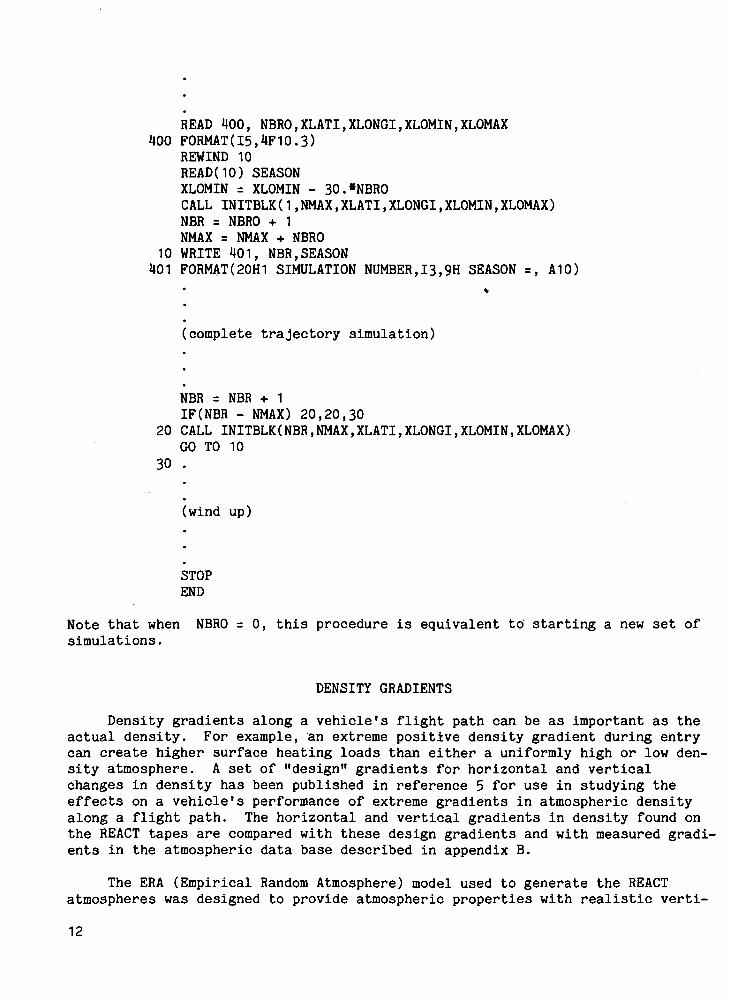
READ 400, NBRO,XLATI,XLONGI,XLOMIN,XLOMAX400 FORMAT(I5,4F10.3)

REWIND 10READ(10) SEASONXLOMIN = XLOMIN - 30.«NBROCALL INITBLK(1,NMAX,XLATI,XLONGI,XLOMIN,XLOMAX)NBR = NBRO + 1NMAX = NMAX + NBRO

10 WRITE 401, NBR,SEASON401 FORMAT(20H1 SIMULATION NUMBER,13,9H SEASON =, A10)

(complete trajectory simulation)

NBR = NBR + 1IF(NBR - NMAX) 20,20,30

20 CALL INITBLK(NBR,NMAX,XLATI,XLONGI,XLOMIN,XLOMAX)GO TO 10

30 .

(wind up)

STOPEND

Note that when NBRO = 0, this procedure is equivalent to starting a new set ofsimulations.

DENSITY GRADIENTS

Density gradients along a vehicle's flight path can be as important as theactual density. For example, an extreme positive density gradient during entrycan create higher surface heating loads than either a uniformly high or low den-sity atmosphere. A set of "design" gradients for horizontal and verticalchanges in density has been published in reference 5 for use in studying theeffects on a vehicle's performance of extreme gradients in atmospheric densityalong a flight path. The horizontal and vertical gradients in density found onthe REACT tapes are compared with these design gradients and with measured gradi-ents in the atmospheric data base described in appendix B.

The ERA (Empirical Random Atmosphere) model used to generate the REACTatmospheres was designed to provide atmospheric properties with realistic verti-

12

cal gradients. That is, one of the objectives in developing the model was toimitate vertical density gradients in the data base. Thus, vertical densitygradients in the REACT atmospheres are inherently similar to those found in thedata. Figures 7(a) and 7(b) compare the mean and standard deviation of verticaldensity gradients in the data with corresponding properties of modeled gradi-ents. Table I shows the percentage of vertical gradients in both the data andthe model which exceed the "design" gradients of reference 5.

In the case of horizontal density gradients, the data base was of no usesince it consists of isolated one-dimensional soundings. In creating the REACTtapes, control of horizontal gradients was exercised by the choice of longitude-latitude grid size and by correlating density profiles which are relativelyclose together. A telephone contact with one of the contributors^ to refer-ence 5 revealed that horizontal design gradients were based on the conclusionin reference 6 that hot and cold atmospheric regimes can occur within 1111.2 km(600 n. mi. or 10° of latitude) of one another. For the construction of thethree-dimensional REACT atmospheres, this statement was interpreted as meaningthat the minimum distance between two statisticlly independent profiles is1111.2 km.

A spacing of 10° was chosen for the longitude-latitude grid. Accordingly,constant-latitude lines are 1111.2 km apart and, therefore, profiles on differ-ent latitude lines could be treated as independent. The longitude lines, on theother hand, are 1111.2 km apart at the equator but converge to a single pointat each pole. Thus, profiles at some adjacent grid points were closer than1111.2 km and these had to be correlated. This was accomplished by first gen-erating independent profiles spaced 1111.2 km apart along a constant latitudeline, and interpolating linearly between these to obtain profiles at the gridpoints. This procedure for correlating adjacent profiles is consistent with theoverall scheme of interpolating between horizontal grid points to get a densityor temperature at any arbitrary location.

A comparison was made between the horizontal design density gradients ofreference 5 and the horizontal density gradients in the REACT atmospheres.Table II lists the percentage of horizontal density gradients on the REACT tapeswhich exceed the design gradients. A significant disparity exists because thereis a greater difference between hot and cold atmospheres in the REACT model,even within the same latitude-season category, than in the model used to con-struct the design gradients in reference 5. Since the REACT model is based onan extensive amount of data, it is believed to be more accurate in its represen-tation of these differences.

CONCLUDING REMARKS

The Random Earth Atmosphere Computer Tapes (REACT) are a set of four magne-tic tapes representing four different seasons which can be used to simulatespacecraft and aircraft trajectories through nonstandard atmospheres character-istic of their respective latitudes and seasons. The atmospheric temperaturesand densities on any one tape (season) at the same latitude and altitude form a

nS. Clark Brown, NASA Marshall Space Flight Center, June 7,

13

random sample whose statistical properties match those of observed temperaturesand densities in a data base of over 6000 sounding-rocket and high-altitudemeasurements.

A method is described whereby, with the addition of three subroutinesinvolving approximately 4000 octal storage locations, the tapes can be linked toany existing trajectory simulation program. Depending on the longitudinal rangeof a particular trajectory, between 349 and 361 independent replications of thattrajectory can be made with each tape. Thus, approximately 1400 replicates canbe generated by using all four tapes.

As a trajectory is simulated, a series of "blocks" is read from one of thetapes. Each "block" contains arrays of atmospheric densities and temperatureswhich span a volume 99 km deep, 30° wide in longitude, and 30° long in latitude.Values in the arrays are located at grid points every 3 km in altitude, andevery 10° in longitude and latitude. To obtain atmospheric properties at anyarbitrary point on a trajectory, the subroutines interpolate by using the arraysas three-way tables. Interpolation is linear in all directions except in verti-cal planes of the density array, where linear interpolation is applied to thelogarithm of density.

Vertical density gradients are consistent with those found in the database. Horizontal density gradients are controlled by assuming a minimum dis-tance between uncorrelated profiles of 1111.2 km. In the case of both horizon-tal and vertical density gradients, a significant percentage of the REACT atmo-spheres exceed the "design" gradients of reference 5. It is believed, however,that the REACT density gradients are more representative of realistic gradients.

Langley Research CenterNational Aeronautics and Space AdministrationHampton, VA 23665May 27, 1977

APPENDIX A

SUBROUTINE LISTINGS

The following listings are suggested versions of the three subroutinesINITBLK, READBLK, and ATMOS:

SUBROUTINE INITBLK(NBR,NMAX,XLATI,XLONGI,XLOMIN,XLOMAX):

COMMON/LINK/ DL,NO,XLATO,XLONGO,RHO(34,M) ,TAU(34,M)IF(NBR-1) 1,1,2

1 DL = .001-XLOMINXLONG=XLONGI+DLNMAX=(10800.-XLOMAX-DL)/30.+1.N0=0CALL READBLK(XLATI,XLONG)RETURN

2 DL=DL+30.XLONG=XLONGI+DLCALL READBLK(XLATI,XLONG)RETURNEND

SUBROUTINE READBLK(XLAT,XLONG):

COMMON/LINK/ DL,NO,XLATO,XLONGO,RHO(34,4,4) ,TAU(34,4,4)NCOLS=XLONG/30.NM1=6.«NCOLS+(XLAT+90.)/30.N=NM1+1IF(NMl-NO) 1,5,3

1 DO 2 I=N,NO2 BACKSPACE 10READ(10) NO,XLATO,XLONGO,RHO,TAURETURN

3 NEXT=NO+1DO 4 I=NEXT,NM1

4 READ(10)5 READ(10) NO,XLATO,XLONGO,RHO,TAURETURNEND

SUBROUTINE ATMOS(Z,XLAT,XLONG,D,T,P,S):

COMMON/LINK/ DL,NO,XLATO,XLONGO,RHO(34,4,4) ,TAU(3M,ll)DIMENSION ANS(4)ZKM=Z/1000.IF(Z) 1,2,2

1 PRINT 401,Z,XLAT,XLONG401 FORMAT(/6(2H »)* ALTITUDE=«F10.1* OUTSIDE RANGE»/6(2H *)«AT LATI

1 TUDE »F6.1* AND LONGITUDE »F7.V)C USE ALTERNATE (1962 STANDARD) ATMOSPHERE MODEL

15

APPENDIX A

ZFT=Z/.3048, CALL AT62(ZFT,ANS)

D=515.379»ANS(1)P=U7.880258«ANS(2)T=ANS(3)S=.30l*8«ANS(4)RETURN

2 IFCZKM-99.) 4,3,13 ZKM=98.9H DXLAT=XLAT-XLATOIF(DXLAT) 11,5,5

5 IF(DXLAT-30.) 7,6,116 DXLAT=29.97 DXLONG=XLONG+DL-XLONGOIF(DXLONG) 11,8,8

8 IF(DXLONG-30.) 10,9,119 DXLONG=29.910 I=ZKM/3.+1.

J=DXLAT/10.+1.JP1=J+1K=DXLONG/10.+1.KP1=K+1R1=(3000.»I-Z)/3000.R2=1.-R1RH01=EXP(R1*ALOG(RHO(I,J,K))+R2*ALOG(RHO(IP1,J,K)))RH02=EXP(R1»ALOG(RHO(I,JP1,K))+R2*ALOG(RHO(IP1,JP1,K)))RH03=EXP(R1«ALOG(RHO(I,J,KP1))+R2»ALOG(RHO(IP1,J,KP1)))RHOi<=EXP(R1*ALOG(RHO(I,JP1,KP1))+R2»ALOG(RHO(IP1.,JP1,KP1)))TAU1rR1«TAU(I,J,K)+R2*TAU(IP1,J,K)TAU2=R1*TAU(I,JP1,K)+R2*TAU(IP1,JP1,K)TAU3=R1*TAU(I,J,KP1)+R2*TAU(IP1,J,KP1)TAU4=R1»TAU(I,JP1,KP1)+R2*TAU(IP1,JP1,KP1)R1=(XLATO+10.»J-XLAT)/10.R2=1.-R1RH012=R1«RH01+R2«RH02RH034=R 1 »RH03+R2«RH04TAU12=R1«TAUUR2*TAU2TAU34=R1*TAU3+R2*TAU4R 1 = ( XLONGO+ 1 0 . *K-XLONG-DL ) / 1 0 .R2=1.-R1D=R1«RH012+R2*RH03U

PrT*D/. 00348362S=.069836«SQRT(T)RETURN

11 RLONG=XLONG+DLCALL READBLK(XLAT,RLONG)GO TO UEND

16

APPENDIX B

EMPIRICAL RANDOM ATMOSPHERE MODEL

To construct the model used in generating the REACT atmospheres, a set ofover 6000 rocket and high-altitude soundings of the atmosphere was modeledempirically. The soundings were divided into categories according to the lati-tude and season of the sounding. The five latitude categories

Band , deg

1530456075

Latitudes covered

0° to 22.5° N or S22.5° to 37.5° N or S37.5° to 52.5° N or S52.5° to 67.5° N or S67.5° to 90.0° N or S

correspond to those used in the 1966 Supplemental Atmospheres (ref. 2). Sound-ings which fell into one of the four nonequatorial latitude categories were alsoclassified by their season. The four season categories are:

Season

SpringSummerAutumnWinter

Northern hemisphere



Southern hemisphere



Soundings in the equatorial (15°) band were not classified as to season sinceseasonal differences at these latitudes are negligible. Table III lists theresultant 17 latitude-season categories and the number of soundings which belongsto each category.

Each sounding was converted, by interpolation, to a temperature and/ordensity profile with observations every 3 km in altitude over the range of thesounding. Since the soundings did not always cover the same altitude range and,in fact, some did not even overlap, the number of observations at each altitudewas always less than the number of profiles shown in table III. Table IV showsthe actual number of temperature observations at each altitude, and table Vshows the number of density observations at each altitude.

A drastic reduction in available data above 60 km is readily apparent.In categories where temperature data were completely missing, temperaturemeans were estimated by using gradients from the 1966 Supplemental Atmospheres(ref. 2) and variances at the highest altitude where data were available wereextended to 99 km. Missing pressure and density means were then filled in byusing the hydrostatic equation and the equation of state, and their varianceswere also extended from lower altitudes. The modeling procedure is describedin detail in reference U. Only a brief description of the model statisticsrelative to the data is given here.

17

APPENDIX B

For the kth season (k = 1, 2, 3, and 4) and any latitude <J>, the model usesa random-number-generating scheme to produce a temperature-altitude profile. Atany fixed altitude_ z the temperature is assumed to be a Gaussian random vari-able with a mean f(z,k,<|>) and a standard deviation s(z,k,<j>); these values areestimated from the data. Thus, model-generated temperature profiles were pro-vided, within the accuracy of the random number generator, the same means andstandard deviations as the temperature data at corresponding altitudes, seasons,and latitudes. Furthermore, within the same profile, temperatures at differentaltitudes were correlated by using coefficients of correlation estimated fromthe data. This latter covariance property insures that modeled vertical tempera-ture gradients are consistent with those in the data.

If |<t>| g 15°, parameters from the 15° band data are used, and likewise,if |<j)| £ 75°, parameters from one of the 75° bands are used depending on theseason . For 15° < |<l>| < 75°, T(z,k,<|>) and sOz,k,<J>) are obtained by linearinterpolation over <j> by using the tables for T and s in the "category"latitudes 15°, 30°, 45°, 60°, and 75°.

In order to calculate pressure and density profiles consistent with a par-ticular random temperature profile, hydrostatic equilibrium is assumed to exist.Thus, pressures vary according to the hydrostatic equation

dP = -gp dz (B1)

where g and p are gravitational acceleration and density, respectively, ataltitude z. By relating temperature, pressure, and density by the equation ofstate

P = W£ (B2)RT

one can calculate complete pressure and density profiles from a given tempera-ture profile and a base pressure Po. Base pressure Po (at sea level) isselected by using a Gaussian random number generator and is correlated to sea-level temperature. Although it is known that hydrostatic equilibrium is notalways maintained, means and standard deviations of model-generated pressuresand densities (based on hydrostatic equilibrium) agree reasonably well with thedata. (See ref. 4.)

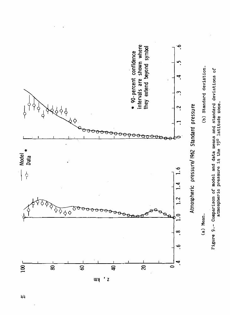
Figure 8, which compares the mean and standard deviation of temperatures inthe model and the data, illustrates the agreement between model and data. Theresults shown here for the 15° latitude-season category are typical of all thecategories. Model statistics in figure 8 and in subsequent figures are based ona sample of 1000 model-generated atmospheres. Figure 9 compares model and datameans and standard deviations of P/?62 where atmospheric pressure P is non-dimensionalized by the 1962 Standard Atmosphere pressure Pfe- Figure 10 com-pares means and standard deviations of nondimensionalized densities P/P62.

18

REFERENCES

1. U.S. Standard Atmosphere, 1962. NASA, U.S. Air Force, and U.S. Weather Bur.,Dec. 1962.

2. U.S. Standard Atmosphere Supplements, 1966. Environ. Sci. Serv. Admin.,NASA, and U.S. Air Force.

3.'U.S. Standard Atmosphere, 1976. NOAA, NASA, and U.S. Air Force, Oct. 1976.

4. Campbell, Janet W.: A Model for Simulating Random Atmospheres as a Functionof Latitude, Season, and Time. NASA TN D-8470, 1977-

5. Daniels, Glenn E., ed.: Terrestrial Environment (Climatic) Criteria Guide-lines for Use in Aerospace Vehicle Development, 1973 Revision. NASATM X-64757, 1973-

6. Cole, Allen E.; and Kantor, Arthur J.: Horizontal and Vertical Distributionsof Atmospheric Density, Up to 90 km. AFCRL-64-483, U.S. Air Force, June1964. (Available from DDC as AD 605196.)

19

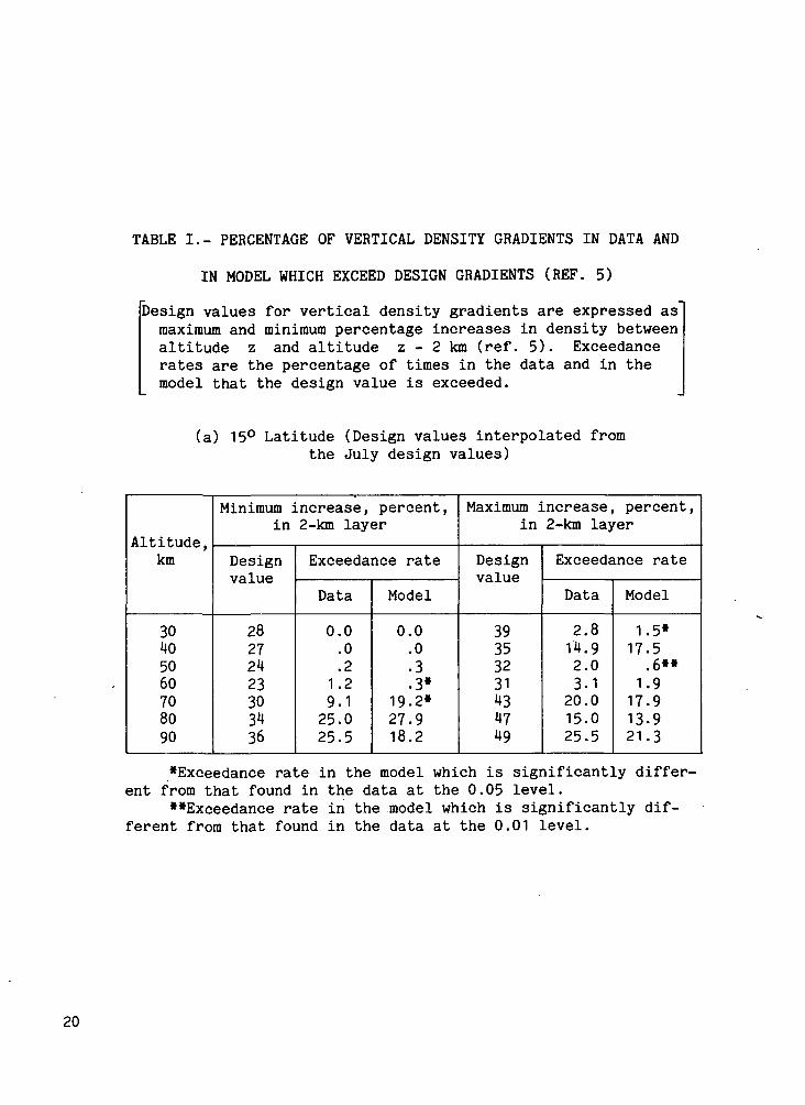
TABLE I.- PERCENTAGE OF VERTICAL DENSITY GRADIENTS IN DATA AND

IN MODEL WHICH EXCEED DESIGN GRADIENTS (REF. 5)

Design values for vertical density gradients are expressed asmaximum and minimum percentage increases in density betweenaltitude z and altitude z - 2 km (ref. 5). Exceedancerates are the percentage of times in the data and in themodel that the design value is exceeded.

(a) 15° Latitude (Design values interpolated fromthe July design values)

Altitude,km

30405060708090

Minimum increase, percent,in 2-km layer

Design

28272423303436

Exceedance rate

Data

0.0.0.2

1.29.125.025.5

Model

0.0.0.3.3*

19. 2»27.918.2

Maximum increase, percent,in 2-km layer

Designvalue

39353231434749

Exceedance rate

Data

2.814.92.03-1

20.015.025.5

Model

1.5*17.5.6**

1.917.913.921.3

"Exceedance rate in the model which is significantly differ-ent from that found in the data at the 0.05 level.

*»Exceedance rate in the model which is significantly dif-ferent from that found in the data at the 0.01 level.

20

TABLE I.- Continued

(b) 30° Latitude

Spring

Altitude,km

30405060708090


Design

30292325333637

Exceedance rate

Data

0.2.3.3

5.166.723.130.0

Model

0.0.1.0

38.0»»76.036.537.9


Designva 1 UP

39373133414750

Exceedance rate

Data

8.31.34.3.4.0 '

7.710.0

Model

6.31.2.9»».0

6.66.121.2

••Exceedance rate in the model which is significantly different from that found in the data at the 0.01 level.

Summer

Altitude,km

30405060708090


Designva 1 IIP

32"282524303040

Exceedance rate

Data

0.3.0

1.14.0

. 37.510.0

.0

Model

0.0.0

1.63-1

71. 2»10.7.2


Designvalue

40353234454750

Exceedance rate

Data

.0.011.32.22.5.0.0

33-3

Model

0.010.5

.6

.66.25.743.2

•Exceedance rate in the model which is significantly differ-ent from that found in the data at the 0.05 level.

21

TABLE I.- Continued

(b) 30° Latitude - Concluded

Autumn

Altitude,km

30405060708090


Design

33272226323540

Exceedance rate

Data

1.0.0.3

10.050.025.038.1

Model

0.0.0.0

11.567.017.239.4


Design

42393231363950

Exceedance rate

Data

0.03.32.84.8

30.025.04.8

Model

0.01.8.7*

2.0*19.333.43.6


Winter

Altitude,km

30405060708090


Designvalue

31282323293026

Exceedance rate

Data

0.21.2.3.0

10.04.8.0

Model

0.0.6.5.3

29.3**•8.9

.0


Designvalue

43403435414760

Exceedance rate

Data

2.01.5.0

1.215.0

.0

.0

Model

0.1»«1.1.0.0

11.2.1.0

**Exceedance rate in the model which is significantly different from that found in the data at the 0.01 level.

22

TABLE I.- Continued

(c) 45° Latitude

Spring

Altitude,km

30405060 '708090

Minimum increase, percent,in 2 -km layer

Designva 1 IIP

32312525273538

Exceedance rate

Data

0.012.2

.09.110.055.6

.0

Model

0.013.01.32.78.538.529.6


Design

38342930415358

Exceedance rate

Data

35.726.728.511.7

.022.250.0

Model

35.327.130.64.7.4

11.87.7

Summer

Altitude,km

30405060708090


Designvalue

34302525263038

Exceedance rate

Data

0.0.0

2.35.6.0

30.8.0

Model

0.0.9

6.6»3.014.927-333. 9»


Designvalue

38353130455356

Exceedance rate

Data

6.111.52.34.27.1.0

37.5

Model

4.614.75.04.016.0

.524.5


23

TABLE I.- Continued

(c) 45° Latitude - Concluded

Autumn

Altitude,km

30405060708090


Design

35262424283540

Exceedance rate

Data

2.9.0.0

2.042.950.050.0

Model

3.7 ..0.0.1»

27.565.266.0


Design

50403434414456

Exceedance rate

Data

0.01.9.0.0.0.0.0

Model

0.0.1«.0.0.4

1.1.1


Winter

Altitude,km

30405060708090


„

Designvalue

35272322191923

Exceedance rate

Data

3.3.0

2.23.8.0.0.0

Model

2.9.3.7.8.8

2.24.5


DesignVfl 1 IIP

474542 .38485562

Exceedance rate

Data

0.0.0.0.0

13.3.0.0

Model

0.0.0.0.2

2.8.9

2.3

24

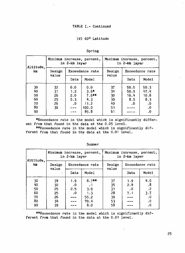
TABLE I.- Continued

(d) 60° Latitude

Spring

Altitude,km

30405060708090


Design

323126252636

Exceedance rate

Data

0.01.22.05.3.0

Model

0.03.6*7.6**4.311.2100.085.8


Design

37343030405161

Exceedance rate

Data

50.550.916.48.5.0

Model

50.347.410.88.3.0.0.0


""Exceedance rate in the model which is significantly dif-ferent from that found in the data at the 0.01 level.

Summer

Altitude,km

30405060708090


Design

34302525263439

Exceedance rate

Data

1.9.0

2.5.0

Model

8.7**.1

3.91.3

55.270.48.0


Design

37353128395358

Exceedance rate

Data

1.92.4.0

7.1.

Model

4.0.8.2

3.7.0.0.0

**Exceedance rate in the model which is significantly dif-ferent from that found in the data at the 0.01 level.

25

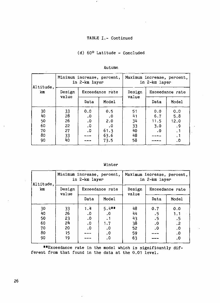
TABLE I.- Continued

(d) 60° Latitude - Concluded

Autumn

Altitude,km

30405060708090


Design

33282622273340

Exceedance rate

Data

0.0.0.0.0.0

Model

0.5.0

2.0.0

61.363.673.5


Design

51413433404858

Exceedance rate

Data

0.06.711.53.0.0

Model

0.05.812.0

.9

.1

.1

.0

Winter

Altitude ,km

30405060708090


Designvalue

33262324201519

Exceedance rate

Data

1.4.0.0.0.0

Model

5.4»».0.1

1.7.0.0.0


DesignVfl 1 IIP

48444338525963

Exceedance rate

Data

0.7.5.5.0.0

Model

0.01.1.5.2.0.0.0

•'Exceedance rate in the model which is significantly dif-ferent from that found in the data at the 0.01 level.

26

TABLE I.- Continued

(e) 75° Latitude

Spring

Altitude,km

30405060708090


Design

29282625283738

Exceedance rate

Data

1.11.4

14.332.44.3

Model

0.01.7

18.241.522.0**51.135.4


Designva 1 IIP

3634333037456.1

Exceedance rate

Data

42.525.7

.018.934.8

Model

41.626.22.09.9

21.07.95.2

••Exceedance rate in the model which is significantly dif-ferent from that found in the data at the 0.01 level.

Summer

Altitude,km

30405060708090


Design

34302524263941

Exceedance rate

Data

23.63-3

24.35.15.4____

Model

19.01.0

16.319.1"29.0"27.935.9


Design

37353327294957

Exceedance rate

Data

3.83.3.0

40.783.8

Model

1.11.2.0

40.042.7««26.426.6

••Exceedance rate in the model which is significantly dif-ferent from that found in the data at the 0.01 level.

27

TABLE I.- Concluded

(e) 75° Latitude - Concluded

Autumn

Altitude,km

30405060708090


Design

30302619272940

Exceedance rate

Data

0.02.93-9.0

9.525.0

Model

0.01.12.6.0

17.227.547.7


Designva T IIP

48413330365157

Exceedance rate

Data

1.319.147.150.028.612.5

'Model

0.018.347.426.3**24.015.411.0


Winter

Altitude ,km

30405060708090


Design

29252227261514

Exceedance rate

Data

0.05.5.0

22.93-85.9

Model

0.0.4

1.032.56.2.1.1


Design

36343330376165

Exceedance rate

Data

2.413.716.3

.0

.05.9

Model

5.124.9**9.5.8.7

1.13.2


28

TABLE II.- PERCENTAGE OF REACT HORIZONTAL DENSITY GRADIENTS WHICH

EXCEED DESIGN GRADIENTS (REF. 5)-

Horizontal gradients measured along lines of constant latitude.Design values for horizontal density gradients are expressedas maximum change in percent departure from 1962 StandardAtmosphere density per 110 km (ref. 5).

(a) Spring tape

Altitude,km

3033363942

4548515457

6063

• 666972

757881848790

REACT density gradients, percent, at latitude -

10° N

Designvalue

0.30.30.30.30.30

.30

.30

.31

.34

.37

.40

.46

.52

.58

.60

.60

.60

.59

.56

.53

.50

Exceedancerate

1924273339

4141464442

4139485557

636468747679

30° N

Designvalue

0.30.36.42.48.52

.55

.58

.58

.52

.46

.40

.52

.64

.76

.86

.951.041.07.98.89.80

Exceedancerate

2323201515

1619222943

5443363945

485154607078

50° N

Designvalue

0.60.60.60.60.66

.75

.84

.90

.90

.90

.901.021.141.261.32

1.351.381.371.281.191.10

Exceedancerate

1217243030

2931343639

3935373837

434855616469

70° N

Designvalue

1.101.04.98.92.84

.75

.66

.58

.52

.46

.40

.46

.52

.58

.62

.65

.68

.66

.54

.42

.30

Exceedancerate

1824324352

6069717780

8582817981

818183909294

29

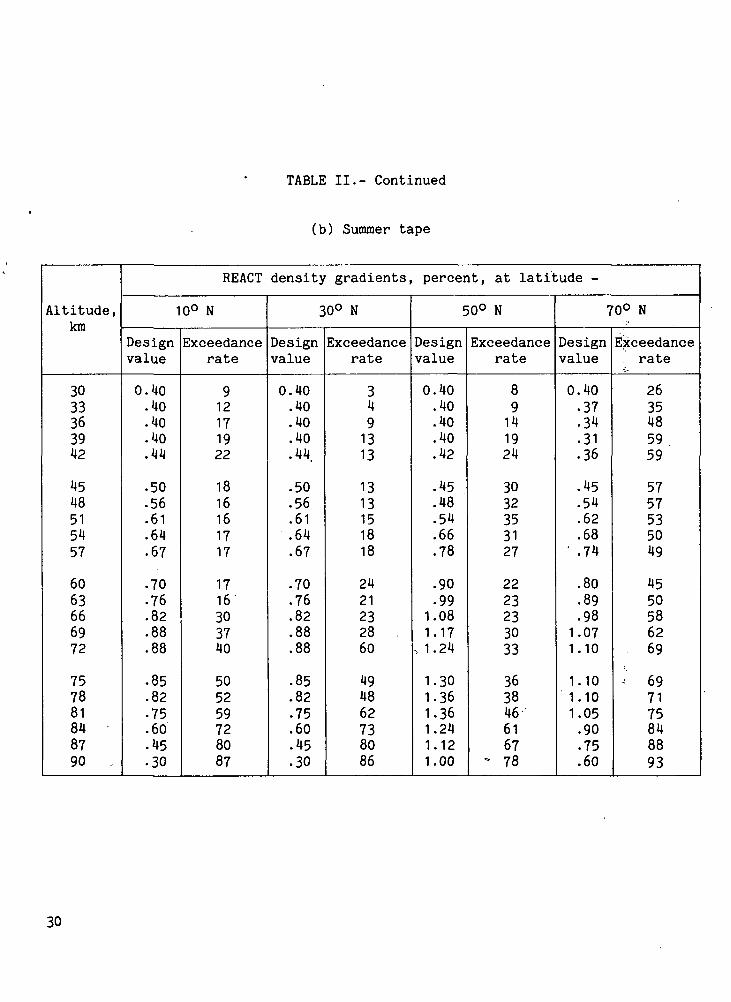
TABLE II.- Continued

(b) Summer tape

Altitude,km

3033363942

4548515457

6063666972

757881848790 .


10° N

Designvalue

0.40.40.40.40.44

• 50• 56.61.64.67

• 70.76.82.88.88

.85

.82

.75

.60

.45

.30

Exceedancerate

912171922

1816161717

1716303740

505259728087

30° N

Designvalue

0.40.40.40.40.44

.50

.56

.61

.64

.67

• 70.76.82.88.88

.85

.82

.75

.60

.45

.30

Exceedancerate

3491313

1313151818

2421232860

494862738086

50° N

Designvalue

0.40.40.40.40.42

.45

.48

.54

.66

.78

.90

.991.081.17

, 1.24

1.301.361.361.241.121.00

Exceedancerate

89141924

3032353127

2223233033

3638466167

- 78

70° N

Designvalue

0.40.37• 34.31• 36

.45

.54

.62

.68' .74

.80

.89

.981.071.10

1.101.101.05.90.75.60

Exceedancerate

2635485959

5757535049

4550586269

-' 697175848893

30

TABLE II.- Continued

(c) Autumn tape

Altitude,km

3033363942

4548515457

6063666972

757881848790


10° N

Designvalue

0.30• 30.30• 30-34

.40

.46

.52

.58

.64

.70

.70

.70

.70

.70

.70

.70

.68

.62

.56

.50

Exceedance- rate

1924273333

2723222118

1720364750

575963717578

30° N

Designvalue

0.30• 30• 30• 30.40

.55

.70

.81

.84

.87

• 90.84.78.72.70

.70

.70

.68

.62

.56

.50

Exceedancerate

2531404739

3124212323

2530314662

636464697881

50° N

Designvalue

0.90.90.90.90.96

1.051.141.221.281.34

1.401.461.521.581.64

1.701.761.781.721.661.60

Exceedancerate

2591519

1922232223

2323222627

302632421351

70° N

Designvalue

1.101.071.041.011.00

1.001.00.99.96• 93

.901.051.201.351.42

1.451.481.451.301.151.00

Exceedancerate

2128364548

5155575860

6257

. 514648

495460687480

31

TABLE II.- Concluded

(d) Winter tape

Altitude,km

3033363942

4548515457

606366 •6972

757881848790


10° N

Designvalue

0.40.40.40.40.40

.40

.40

.44

.56

.68

.80

.83

.86

.89

.94

1.001.061.07.98-89.80

Exceedancerate

912171926

2730302216

1213273636

433946576269

30° N

Designvalue

0.40.46.52.58.66

.75

.84

.92

.981.04

1.101.251.401.551.64

1.701.761-751.601.451.30

Exceedancerate

1111171310

10991010

9551415

142329364755

50° N

Designvalue

1.601.661.721.781.92

2.102.282.452.602.75

2.902.902.902.902.86

2.802.742.612.342.071.80

Exceedancerate

00111

11111

11125

7814273650

70° N

Designvalue

2.602.722.842.962.92

2.802.682.562.442.32

2.202.232.262.292.28

2.252.222.152.001.851.70

Exceedancerate

00247

914171618

2017161417

192534445259

32

TABLE III.- NUMBER OF PROFILES IN DATA BASE FOR

EACH LATITUDE-SEASON CATEGORY

Latitude band

15°

30°

1450

60°

75°

Profiles in season -

Spring Summer Autumn Winter

'1928

495

184

238

101

468

193

176

128

516

154

217

91

504

147

342

122

Total

1928

1983

678

973

442

6004

33

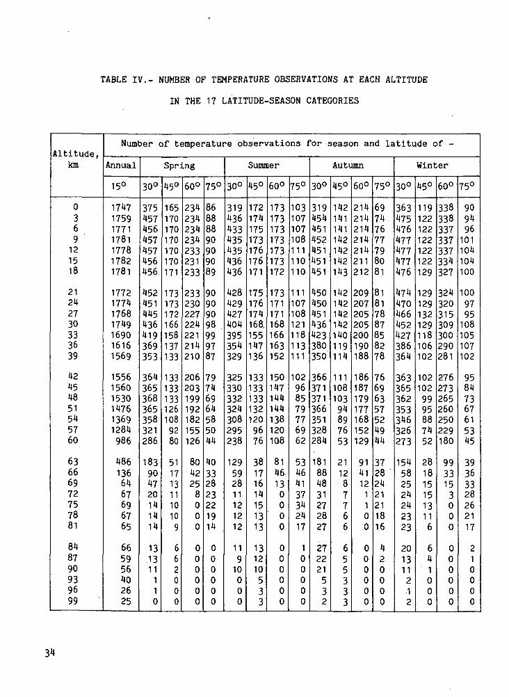
TABLE IV.- NUMBER OF TEMPERATURE OBSERVATIONS AT EACH ALTITUDE

IN THE 17 LATITUDE-SEASON CATEGORIES

Altitude,km

0369121518

21242730333639

42454851545760

63666972757881

848790939699

Number of temperature observations for season and latitude of -

Annual

15°

1747175917711781177817821781

1772177417681749169016161569

155615601530147613691284986

4861366467696765

665956402625

Spring

30°

375457456457457456456

452451445436419369353

364365368365358321286

183904720141414

13.1311110

45°

165170170170170170171

173173172166158137133

1331331331261089280

5117131110109

662000

60°

234234234234233231233

233230227224221214210

206203199192182155126

8042258000

000000

75°

86888890909089

90909098999787

79746964585044

40332823221914

000000

Summer

30°

319436433435435436436

428429427404395354329

325330332324308295238

129592811121212

11910000

45°

172174175173176176171

175176174168.155147136

1331331331321209676

38171614151313

131210533

60°

173173173173173173172

173171171168166163152

150147144144138120108

8146130000

000000

75°

103107107108111110110

111107108121118113111

102968579776962

53464137342417

100000

Autumn

30°

319454451452451451451

450450451436423380350

366371371366351328284

181884831272827

272221532

45°

142141141142142142143

142142142142140119114

11110810394897653

211287766

655333

60°

214214214214214211212

209207205205200190188

186187179177168152129

9141121100

000000

75°

69747677798081

81817887858278

76696357524944

37282421211816

420000

Winter

30°

363475476477477477476

474470466452427386364

363365362353346326273

154582524242323

201311212

45°

119122122122122122129

129129132129118106102

1021029995887452

2818151513116

641000

60°

338338337337337334327

324320315309300290281

276273265260250229180

9933153000

000000

75°

909496101104104100

1009795108105107102

95847367615345

39363328262117

210000

TABLE V.- NUMBER OF DENSITY OBSERVATIONS AT EACH ALTITUDE

IN THE 17 LATITUDE-SEASON CATEGORIES

Altitude,km

0369121518

21242730333639

1*2454851545760

63666972757881

848790939699

Number of density observations for season and latitude of -

Annual

15°

1744174817531755173417661762

1748172717101680158014871426

141114091377132812571141870

4231216060666260

615451392624

Spring

30°

372452451449453453453

447447438421400335312

322326328327324292261

168854518131313

121210110

45°

163169170167170169168

170166168157154135131

1311321311231069180

5117121010109

662000

60°

232233233233233231232

232227220216204186171

16916315815214512194

6036228000

000000

75°

86868787878787

88868796969179

71666156504337

36312823221914.

000000

Summer

30°

304431429429424431432

424423417390381325292

285289290289272259202

110512511111011

11910000

45°

1721731741731701662

173174170166151139133

1311291301291179375

38171614151313

13109533

60°

168173173173173173169

170166165162158149131

1271241231201129885

6640110000

000000

75°

102105105103106107W7

107105107118114109103

92867770686359

52464037342417

100000

Autumn

30°

316449449445445447449

445435435415404351309

327332331329313294253

160804631272625

262221532

45°

142140141140142141143

141142140142138117112

10910610192877451

201187766

655333

60°

212214212213214211209

203200198196185165153

150148141139129118101

7234101100

000000

75°

68717274757577

78797684807671

70635651474440

34262321211816

410000

Winter

30°

360473475472476475474

471466459445418367342

338340336329322303254

137552422232322

191311212

45°

119122122122122122129

12812712812711210198

99989693867252

2818151513116

641000

60°

335338337337333332326

320313304289272241230

222222215211202185144

8330153000

000000

75°

8891909510010298

95898699938982

73625249434135

29282826252117

210000

35

s1— t

CM

^

OITNr— 1

CM

V

ooir\

CM

f

fci— ievj

V

*i— iCM

V

i/yif\i— iCM

V\ \[N\

so

oCO

Si-

oo1— 1

CMi— 1

NO

II

0

A

£

0CM

«

i— i

i— Ii— i

ITN

3-

OOCM

CMCM

i— 1

CDi— i

^

N\

CO

1 —CM

i— ICM

i— i

o.

CO

•\

CM

CM

CDCM

i— I

OO

CM

•\

•— 1

CM

Z.

2

l»~

H

3 O CD CD CD CD . C^ NO CO CO NO Cy

1 1 1

A

CDOO

CDIP*i— i

"CDCMf-H

CDO

CDNO

CDCO

CD>n

S1

01co

oJJo3

cd

cordo =U 0)cu -o<! 3E~< 4^

•HC bOO C

O

OO T3rH CjQ CD

CM (1)O T3

C -H0) -Pa ca0) rHbO

CO

Q)

3bO

36

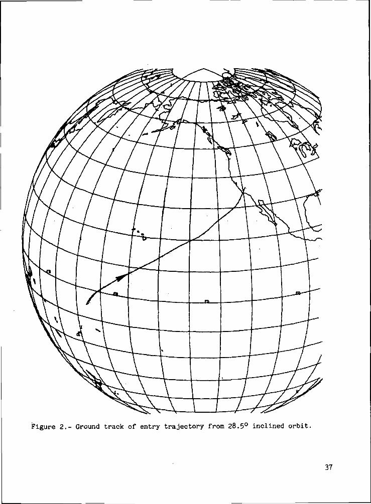
Figure 2.- Ground track of entry trajectory from 28.5° inclined orbit.

37

^ '

CO

00 \lf\

, m>

\

^ \

CO \

\CM

\i— I

\N \_

^

\ '

\\

X\

\ \

\N\\\

*

\

CD

"iZ3

(OO

"5.o>o:

\~

^ ^

•

, x

3 O O O CD O O?• vO CO CO vO 0s

ST

"CD

C3 ^CM •—

C\J

0)

300

•HCM

C

|

co

t. oo <-*J WO 0.0) <C

C?L, C-U O

CM COO X

OCO OQ) <-!

COO O•H -PiHQ. Q)0) >£- -H

40 COC H0) 0)

TD L,C0)a0)73C

Ion0)£-,

6ap '

38

Oi= §

-co

; ,

CO

boC

•Hm3

Sa)L,bOO

at, CO0) O

OO

C, -O W-p Jo ma> a

£-, K

(0 ujO CQ

a M

SH COo a>

<M C•H

.p J->t. 3

3ra

I•

.=r

•HEL,

39

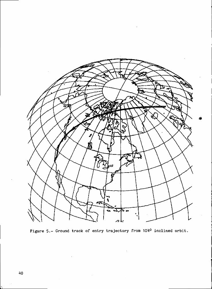
Figure 5.- Ground track of entry trajectory from 104° inclined orbit.

o

I—o

0>.QE o>

i—i O

in0)t*bO•H

oJSco

t- oo «-•P WO Oi0) «a!*r"> EH0)t-, c•P O

4-< COO Jrf

Om o0) r-l4J ^3(0o o•H -P

t, -H-l->

-P CdC ^H0) (1)T3 t,C<UO.(U•o

I

vO

vOC5

6a p '

oNO

I

0

CD -

CDo -^ =c 5 5?CD «/>

11CD

CD

O *- CNJ

IM

03

isl

CCDCD

CO•H

<U•o•Ot,n)•oco

4->co

<Mocoo

a•H

CO 0)•o c

o•O N£-,CO 0)

•O T3c aaj -P4J -Hw -P

n)T3 ^HC(0 Oinco «-C(0 0)<u x:S -Pco c

4-> -rH

_ *CD•a ro° IS

S

ovO

0^a-

c:CD•a

^

CDcncco.CoCDCT>toCCDif c« SQ- s

4->•a cc a>(0 -H

•a^1 OJ0 L.T3 bOoa >>

4-5t_l .4—1 *r-1o co

cc <oo -oCO•H .H{-. n!(0 OO. -Ha -P0 C,O 0)

<=>CNJ

a>

I•H

OOO

OCVJ

LU>| ' Z

o•H4->tO•H

0)•o

o)T3Ccd-PC/3

o>

CDQ.

O>

O)

OE

ccd0)S

CMO

m§•H-PtO•H

0)•a •

Q)•a cfn Otfl N

T3C 0)<0 -O^> 3CO -P

•H73 -P

tO9CO OC 1^^

S <D

a -Pto c•o -H•o o>c t,cd 3

rH fljQ) t,

•O 0)o aS S

CD

oo

C -HO L.co a)•H J3s* aA COa oS SO 4Ju co

oo

0)

I•H

I • I I I - I

o•rH-P<d•H

0>T3

to

I—O-

"Ero

c42

CNJ

I/)<u

O)

o

a1

cd

<M

O

no

•rH

0]

s_,cd•occd4^CO

»••— *,0v-'

0)•oT3 (1)CH Ccd o•O Nccd <u-P -On 3•o THC -Pcd cd(0C 0cd in0) r-S

Q)cd xi•P j->cd•o c•oC CDcd L,

3rH CO0) co•O 0)0 i.B a

0

C 0)O Sco a.•H m

2.1S cdooi•

CTl

0)L,

00•HCb

' Z

•o J2o "Jo

CNI

O•H4->cd

0)•o

cd•O

^ I~ CO

o>•o

03-oCra

t/1

CSJ

ooC

O'i_CD.c-CO.

A0)s

<4H

O

rao•H-Pn)

•o•o •L, a)n) C•o OC Na-u a>ra -o•o *JC -rH

ra rHcn) oa> toB '-cd <D*> £cd -P10 cT3 -H

cd >>

<D ra•o Co wB -o<4H O

O -HL.

C <PO X!ra a.•H rat, ocd 0a -PS cdo

Joo

0)

I•Hfc.

| i I i L

8 OCXJ

' Z

NASA-Langley, 1977 L-10623

NATIONAL AERONAUTICS AND SPACE ADMINISTRATION

WASHINGTON. D.C. 2O546

OFFICIAL BUSINESS

PENALTY FOR PRIVATE USE S3OO SPECIAL FOURTH-CLASS RATEBOOK

POSTAGE AND FEES PAIDNATIONAL AERONAUTICS AND

SPACE ADMINISTRATION4SI

POSTMASTER : If Undeliverable (Section 158Postal Manual) Do Not Return

"The aeronautical and space activities of the United States shall beconducted so as to contribute . . . to the expansion of human knowl-edge of phenomena in the atmosphere and space. The Administrationshall provide for the widest practicable and appropriate disseminationof information concerning its activities and the results thereof."

—NATIONAL AERONAUTICS AND SPACE ACT OF 1958

NASA SCIENTIFIC AND TECHNICAL PUBLICATIONSTECHNICAL REPORTS: Scientific andtechnical information considered important,complete, and a lasting contribution to existingknowledge.

TECHNICAL NOTES: Information less broadin scope but nevertheless of importance as acontribution to existing knowledge.

TECHNICAL MEMORANDUMS:Information receiving limited distributionbecause of preliminary data, security classifica-tion, or other reasons. Also includes conferenceproceedings with either limited or unlimiteddistribution.

CONTRACTOR REPORTS: Scientific andtechnical information generated under a NASAcontract or grant and considered an importantcontribution to existing knowledge.

TECHNICAL TRANSLATIONS: Informationpublished in a foreign language consideredto merit NASA distribution in English.

SPECIAL PUBLICATIONS: Informationderived from or of value to NASA activities.Publications include final reports of majorprojects, monographs, data compilations,handbooks, sourcebooks, and specialbibliographies.

TECHNOLOGY UTILIZATIONPUBLICATIONS: Information on technologyused by NASA that may be of particularinterest in commercial and other non-aerospaceapplications. Publications include Tech Briefs,Technology Utilization Reports andTechnology Surveys.

Details on the availability of these publications may be obfoined from:

' SCIENTIFIC AND TECHNICAL INFORMATION OFFICE

NATIONAL A E R O N A U T I C S AND S P A C E ADMINISTRATIONWashington, D.C. 20546

case fil copy - nasa · mately 1000 (octal) words. ... nbro number of trajectories already...

Documents