cascading bandits: learning to rank in the cascade model · cascading bandits: learning to rank in...

Cascading Bandits: Learning to Rank in the Cascade Model

Branislav Kveton [email protected]

Adobe Research, San Jose, CA

Csaba Szepesvari [email protected]

Department of Computing Science, University of Alberta

Zheng Wen [email protected]

Yahoo Labs, Sunnyvale, CA

Azin Ashkan [email protected]

Technicolor Research, Los Altos, CA

AbstractA search engine usually outputs a list of K webpages. The user examines this list, from the firstweb page to the last, and chooses the first attrac-tive page. This model of user behavior is knownas the cascade model. In this paper, we proposecascading bandits, a learning variant of the cas-cade model where the objective is to identify Kmost attractive items. We formulate our problemas a stochastic combinatorial partial monitoringproblem. We propose two algorithms for solvingit, CascadeUCB1 and CascadeKL-UCB. We alsoprove gap-dependent upper bounds on the regretof these algorithms and derive a lower bound onthe regret in cascading bandits. The lower boundmatches the upper bound of CascadeKL-UCB upto a logarithmic factor. We experiment with ouralgorithms on several problems. The algorithmsperform surprisingly well even when our model-ing assumptions are violated.

1. IntroductionThe cascade model is a popular model of user behavior inweb search (Craswell et al., 2008). In this model, the useris recommended a list of K items, such as web pages. Theuser examines the recommended list from the first item tothe last, and selects the first attractive item. In web search,this is manifested as a click. The items before the first at-tractive item are not attractive, because the user examinesthese items but does not click on them. The items after the

Proceedings of the 32nd International Conference on MachineLearning, Lille, France, 2015. JMLR: W&CP volume 37. Copy-right 2015 by the author(s).

first attractive item are unobserved, because the user neverexamines these items. The optimal list, the list of K itemsthat maximizes the probability that the user finds an attrac-tive item, are K most attractive items. The cascade modelis simple but effective in explaining the so-called positionbias in historical click data (Craswell et al., 2008). There-fore, it is a reasonable model of user behavior.

In this paper, we propose an online learning variant of thecascade model, which we refer to as cascading bandits. Inthis model, the learning agent does not know the attractionprobabilities of items. At time t, the agent recommends tothe user a list of K items out of L items and then observesthe index of the item that the user clicks. If the user clickson an item, the agent receives a reward of one. The goal ofthe agent is to maximize its total reward, or equivalently tominimize its cumulative regret with respect to the list of Kmost attractive items. Our learning problem can be viewedas a bandit problem where the reward of the agent is a partof its feedback. But the feedback is richer than the reward.Specifically, the agent knows that the items before the firstattractive item are not attractive.

We make five contributions. First, we formulate a learningvariant of the cascade model as a stochastic combinatorialpartial monitoring problem. Second, we propose two algo-rithms for solving it, CascadeUCB1 and CascadeKL-UCB.CascadeUCB1 is motivated by CombUCB1, a computation-ally and sample efficient algorithm for stochastic combina-torial semi-bandits (Gai et al., 2012; Kveton et al., 2015).CascadeKL-UCB is motivated by KL-UCB and we expect itto perform better when the attraction probabilities of itemsare low (Garivier & Cappe, 2011). This setting is commonin the problems of our interest, such as web search. Third,we prove gap-dependent upper bounds on the regret of ouralgorithms. Fourth, we derive a lower bound on the regret

arX

iv:1

502.

0276

3v2

[cs

.LG

] 1

8 M

ay 2

015


in cascading bandits. This bound matches the upper boundof CascadeKL-UCB up to a logarithmic factor. Finally, weexperiment with our algorithms on several problems. Theyperform well even when our modeling assumptions are notsatisfied.

Our paper is organized as follows. In Section 2, we reviewthe cascade model. In Section 3, we introduce our learningproblem and propose two UCB-like algorithms for solvingit. In Section 4, we derive gap-dependent upper bounds onthe regret of CascadeUCB1 and CascadeKL-UCB. In addi-tion, we prove a lower bound and discuss how it relates toour upper bounds. We experiment with our learning algo-rithms in Section 5. In Section 6, we review related work.We conclude in Section 7.

2. BackgroundWeb pages in a search engine can be ranked automaticallyby fitting a model of user behavior in web search from his-torical click data (Radlinski & Joachims, 2005; Agichteinet al., 2006). The user is typically assumed to scan a list ofK web pages A = (a1, . . . , aK), which we call items. Theitems belong to some ground set E = 1, . . . , L, such asthe set of all web pages. Many models of user behavior inweb search exist (Becker et al., 2007; Craswell et al., 2008;Richardson et al., 2007). Each of them explains the clicksof the user differently. We focus on the cascade model.

The cascade model is a popular model of user behavior inweb search (Craswell et al., 2008). In this model, the userscans a list of K items A = (a1, . . . , aK) ∈ ΠK(E) fromthe first item a1 to the last aK , where ΠK(E) is the set ofall K-permutations of set E. The model is parameterizedby attraction probabilities w ∈ [0, 1]E . After the user ex-amines item ak, the item attracts the user with probabilityw(ak), independently of the other items. If the user is at-tracted by item ak, the user clicks on it and does not exam-ine the remaining items. If the user is not attracted by itemak, the user examines item ak+1. It is easy to see that theprobability that item ak is examined is

∏k−1i=1 (1 − w(ai)),

and that the probability that at least one item in A is attrac-tive is 1−

∏Ki=1(1− w(ai)). This objective is maximized

by K most attractive items.

The cascade model assumes that the user clicks on at mostone item. In practice, the user may click on multiple items.The cascade model cannot explain this pattern. Therefore,the model was extended in several directions, for instanceto take into account multiple clicks and the persistence ofusers (Chapelle & Zhang, 2009; Guo et al., 2009a;b). Theextended models explain click data better than the cascademodel. Nevertheless, the cascade model is still very attrac-tive, because it is simpler and can be reasonably fit to clickdata. Therefore, as a first step towards understanding morecomplex models, we study an online variant of the cascade

model in this work.

3. Cascading BanditsWe propose a learning variant of the cascade model (Sec-tion 3.1) and two computationally-efficient algorithms forsolving it (Section 3.2). To simplify exposition, all randomvariables are written in bold.

3.1. Setting

We refer to our learning problem as a generalized cascad-ing bandit. Formally, we represent the problem by a tupleB = (E,P,K), where E = 1, . . . , L is a ground set ofL items, P is a probability distribution over a unit hyper-cube 0, 1E , and K ≤ L is the number of recommendeditems. We call the bandit generalized because the form ofthe distribution P has not been specified yet.

Let (wt)nt=1 be an i.i.d. sequence of n weights drawn from

P , where wt ∈ 0, 1E and wt(e) is the preference of theuser for item e at time t. That is, wt(e) = 1 if and only ifitem e attracts the user at time t. The learning agent inter-acts with our problem as follows. At time t, the agent rec-ommends a list of K items At = (at1, . . . ,a

tK) ∈ ΠK(E).

The list is computed from the observations of the agent upto time t. The user examines the list, from the first item at1to the last atK , and clicks on the first attractive item. If theuser is not attracted by any item, the user does not click onany item. Then time increases to t+ 1.

The reward of the agent at time t can be written in severalforms. For instance, as maxkwt(a

tk), at least one item in

list At is attractive; or as f(At,wt), where:

f(A,w) = 1−K∏k=1

(1− w(ak)) ,

A = (a1, . . . , aK) ∈ ΠK(E), and w ∈ 0, 1E . This lateralgebraic form is particularly useful in our proofs.

The agent at time t receives feedback:

Ct = arg min

1 ≤ k ≤ K : wt(atk) = 1

,

where we assume that arg min ∅ = ∞. The feedback Ct

is the click of the user. If Ct ≤ K, the user clicks on itemCt. If Ct =∞, the user does not click on any item. Sincethe user clicks on the first attractive item in the list, we candetermine the observed weights of all recommended itemsat time t from Ct. In particular, note that:

wt(atk) = 1Ct = k k = 1, . . . ,min Ct,K . (1)

We say that item e is observed at time t if e = atk for some1 ≤ k ≤ min Ct,K.


In the cascade model (Section 2), the weights of the itemsin the ground set E are distributed independently. We alsomake this assumption.

Assumption 1. The weights w are distributed as:

P (w) =∏e∈E

Pe(w(e)) ,

where Pe is a Bernoulli distribution with mean w(e).

Under this assumption, we refer to our learning problem asa cascading bandit. In this new problem, the weight of anyitem at time t is drawn independently of the weights of theother items at that, or any other, time. This assumption hasprofound consequences and leads to a particularly efficientlearning algorithm in Section 3.2. More specifically, underour assumption, the expected reward for list A ∈ ΠK(E),the probability that at least one item in A is attractive, canbe expressed as E [f(A,w)] = f(A, w), and depends onlyon the attraction probabilities of individual items in A.

The agent’s policy is evaluated by its expected cumulativeregret:

R(n) = E

[n∑t=1

R(At,wt)

],

where R(At,wt) = f(A∗,wt)− f(At,wt) is the instan-taneous stochastic regret of the agent at time t and:

A∗ = arg maxA∈ΠK(E)

f(A, w)

is the optimal list of items, the list that maximized the re-ward at any time t. Since f is invariant to the permutationof A, there exist at least K! optimal lists. For simplicity ofexposition, we assume that the optimal solution, as a set, isunique.

3.2. Algorithms

We propose two algorithms for solving cascading bandits,CascadeUCB1 and CascadeKL-UCB. CascadeUCB1 is mo-tivated by UCB1 (Auer et al., 2002) and CascadeKL-UCB ismotivated by KL-UCB (Garivier & Cappe, 2011).

The pseudocode of both algorithms is in Algorithm 1. Thealgorithms are similar and differ only in how they estimatethe upper confidence bound (UCB) Ut(e) on the attractionprobability of item e at time t. After that, they recommenda list of K items with largest UCBs:

At = arg maxA∈ΠK(E)

f(A,Ut) . (2)

Note that At is determined only up to a permutation of theitems in it. The payoff is not affected by this ordering. Butthe observations are. For now, we leave the order of items

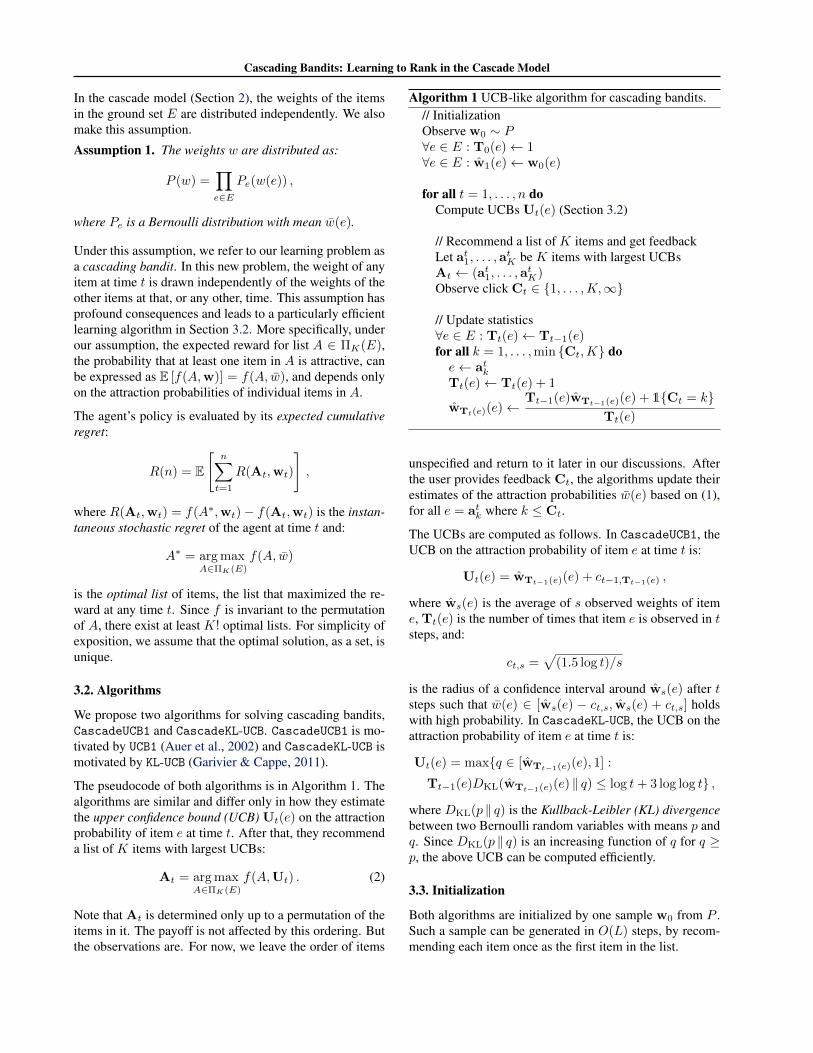
Algorithm 1 UCB-like algorithm for cascading bandits.// InitializationObserve w0 ∼ P∀e ∈ E : T0(e)← 1∀e ∈ E : w1(e)← w0(e)

for all t = 1, . . . , n doCompute UCBs Ut(e) (Section 3.2)

// Recommend a list of K items and get feedbackLet at1, . . . ,a

tK be K items with largest UCBs

At ← (at1, . . . ,atK)

Observe click Ct ∈ 1, . . . ,K,∞

// Update statistics∀e ∈ E : Tt(e)← Tt−1(e)for all k = 1, . . . ,min Ct,K doe← atkTt(e)← Tt(e) + 1

wTt(e)(e)←Tt−1(e)wTt−1(e)(e) + 1Ct = k

Tt(e)

unspecified and return to it later in our discussions. Afterthe user provides feedback Ct, the algorithms update theirestimates of the attraction probabilities w(e) based on (1),for all e = atk where k ≤ Ct.

The UCBs are computed as follows. In CascadeUCB1, theUCB on the attraction probability of item e at time t is:

Ut(e) = wTt−1(e)(e) + ct−1,Tt−1(e) ,

where ws(e) is the average of s observed weights of iteme, Tt(e) is the number of times that item e is observed in tsteps, and:

ct,s =√

(1.5 log t)/s

is the radius of a confidence interval around ws(e) after tsteps such that w(e) ∈ [ws(e) − ct,s, ws(e) + ct,s] holdswith high probability. In CascadeKL-UCB, the UCB on theattraction probability of item e at time t is:

Ut(e) = maxq ∈ [wTt−1(e)(e), 1] :

Tt−1(e)DKL(wTt−1(e)(e) ‖ q) ≤ log t+ 3 log log t ,

where DKL(p ‖ q) is the Kullback-Leibler (KL) divergencebetween two Bernoulli random variables with means p andq. Since DKL(p ‖ q) is an increasing function of q for q ≥p, the above UCB can be computed efficiently.

3.3. Initialization

Both algorithms are initialized by one sample w0 from P .Such a sample can be generated in O(L) steps, by recom-mending each item once as the first item in the list.


4. AnalysisOur analysis exploits the fact that our reward and feedbackmodels are closely connected. More specifically, we showin Section 4.1 that the learning algorithm can suffer regretonly if it recommends suboptimal items that are observed.Based on this result, we prove upper bounds on the n-stepregret of CascadeUCB1 and CascadeKL-UCB (Section 4.2).We prove a lower bound on the regret in cascading banditsin Section 4.3. We discuss our results in Section 4.4.

4.1. Regret Decomposition

Without loss of generality, we assume that the items in theground set E are sorted in decreasing order of their attrac-tion probabilities, w(1) ≥ . . . ≥ w(L). In this setting, theoptimal solution is A∗ = (1, . . . ,K), and contains the firstK items in E. We say that item e is optimal if 1 ≤ e ≤ K.Similarly, we say that item e is suboptimal if K < e ≤ L.The gap between the attraction probabilities of suboptimalitem e and optimal item e∗:

∆e,e∗ = w(e∗)− w(e) (3)

measures the hardness of discriminating the items. When-ever convenient, we view an ordered list of items as the setof items on that list.

Our main technical lemma is below. The lemma says thatthe expected value of the difference of the products of ran-dom variables can be written in a particularly useful form.Lemma 1. Let A = (a1, . . . , aK) and B = (b1, . . . , bK)be any two lists of K items from ΠK(E) such that ai = bjonly if i = j. Let w ∼ P in Assumption 1. Then:

E

[K∏k=1

w(ak)−K∏k=1

w(bk)

]=

K∑k=1

E

[k−1∏i=1

w(ai)

]×

E [w(ak)−w(bk)]

K∏j=k+1

E [w(bj)]

.

Proof. The claim is proved in Appendix B.

Let:

Ht = (A1,C1, . . . ,At−1,Ct−1,At) (4)

be the history of the learning agent up to choosing At, thefirst t− 1 observations and t actions. Let Et [·] = E [· |Ht]be the conditional expectation given historyHt. We boundEt [R(At,wt)], the expected regret conditioned on historyHt, as follows.Theorem 1. For any item e and optimal item e∗, let:

Ge,e∗,t = ∃1 ≤ k ≤ K s.t. atk = e, πt(k) = e∗, (5)

wt(at1) = . . . = wt(a

tk−1) = 0

be the event that item e is chosen instead of item e∗ at timet, and that item e is observed. Then there exists a permuta-tion πt of optimal items 1, . . . ,K, which is a determin-istic function of Ht, such that Ut(a

tk) ≥ Ut(πt(k)) for all

k. Moreover:

Et [R(At,wt)] ≤L∑

e=K+1

K∑e∗=1

∆e,e∗Et [1Ge,e∗,t]

Et [R(At,wt)] ≥ αL∑

e=K+1

K∑e∗=1

∆e,e∗ Et [1Ge,e∗,t] ,

where α = (1−w(1))K−1 and w(1) is the attraction prob-ability of the most attractive item.

Proof. We define πt as follows. For any k, if the k-th itemin At is optimal, we place this item at position k, πt(k) =atk. The remaining optimal items are positioned arbitrarily.Since A∗ is optimal with respect to w, w(atk) ≤ w(πt(k))for all k. Similarly, since At is optimal with respect to Ut,Ut(a

tk) ≥ Ut(πt(k)) for all k. Therefore, πt is the desired

permutation.

The permutation πt reorders the optimal items in a conve-nient way. Since time t is fixed, let a∗k = πt(k). Then:

Et [R(At,wt)] =

Et

[K∏k=1

(1−wt(atk))−

K∏k=1

(1−wt(a∗k))

].

Now we exploit the fact that the entries of wt are indepen-dent of each other given Ht. By Lemma 1, we can rewritethe right-hand side of the above equation as:

K∑k=1

Et

[k−1∏i=1

(1−wt(ati))

]Et[wt(a

∗k)−wt(a

tk)]× K∏

j=k+1

Et[1−wt(a

∗j )] .

Note that Et [wt(a∗k)−wt(a

tk)] = ∆atk,a

∗k. Furthermore,∏k−1

i=1 (1−wt(ati)) = 1

Gatk,a

∗k,t

by conditioning onHt.

Therefore, we get that Et [R(At,wt)] is equal to:

K∑k=1

∆atk,a∗kEt[1Gatk,a

∗k,t

] K∏j=k+1

Et[1−wt(a

∗j )].

By definition of πt, ∆atk,a∗k

= 0 when item atk is optimal.In addition, 1 − w(1) ≤ Et

[1−wt(a

∗j )]≤ 1 for any op-

timal a∗j . Our upper and lower bounds on Et [R(At,wt)]follow from these observations.


4.2. Upper Bounds

In this section, we derive two upper bounds on the n-stepregret of CascadeUCB1 and CascadeKL-UCB.

Theorem 2. The expected n-step regret of CascadeUCB1is bounded as:

R(n) ≤L∑

e=K+1

12

∆e,Klog n+

π2

3L .

Proof. The complete proof is in Appendix A.1. The proofhas four main steps. First, we bound the regret of the eventthat w(e) is outside of the high-probability confidence in-terval around wTt−1(e)(e) for at least one item e. Second,we decompose the regret at time t and apply Theorem 1 tobound it from above. Third, we bound the number of timesthat each suboptimal item is chosen in n steps. Fourth, wepeel off an extra factor of K in our upper bound based onKveton et al. (2014a). Finally, we sum up the regret of allsuboptimal items.

Theorem 3. For any ε > 0, the expected n-step regret ofCascadeKL-UCB is bounded as:

R(n) ≤L∑

e=K+1

(1 + ε)∆e,K(1 + log(1/∆e,K))

DKL(w(e) ‖ w(K))×

(log n+ 3 log log n) + C ,

where C = KLC2(ε)nβ(ε)

+ 7K log log n, and the constantsC2(ε) and β(ε) are defined in Garivier & Cappe (2011).

Proof. The complete proof is in Appendix A.2. The proofhas four main steps. First, we bound the regret of the eventthat w(e) > Ut(e) for at least one optimal item e. Second,we decompose the regret at time t and apply Theorem 1 tobound it from above. Third, we bound the number of timesthat each suboptimal item is chosen in n steps. Fourth, wederive a new peeling argument for KL-UCB (Lemma 2) andeliminate an extra factor of K in our upper bound. Finally,we sum up the regret of all suboptimal items.

4.3. Lower Bound

Our lower bound is derived on the following problem. Theground set contains L items E = 1, . . . , L. The distribu-tion P is a product of L Bernoulli distributions Pe, each ofwhich is parameterized by:

w(e) =

p e ≤ Kp−∆ otherwise ,

(6)

where ∆ ∈ (0, p) is the gap between any optimal and sub-optimal items. We refer to the resulting bandit problem asBLB(L,K, p,∆); and parameterize it by L, K, p, and ∆.

Our lower bound holds for consistent algorithms. We saythat the algorithm is consistent if for any cascading bandit,any suboptimal listA, and any α > 0, E [Tn(A)] = o(nα),where Tn(A) is the number of times that list A is recom-mended in n steps. Note that the restriction to the consis-tent algorithms is without loss of generality. The reason isthat any inconsistent algorithm must suffer polynomial re-gret on some instance of cascading bandits, and thereforecannot achieve logarithmic regret on every instance of ourproblem, similarly to CascadeUCB1 and CascadeKL-UCB.Theorem 4. For any cascading bandit BLB, the regret ofany consistent algorithm is bounded from below as:

lim infn→∞

R(n)

log n≥ (L−K)∆(1− p)K−1

DKL(p−∆ ‖ p).

Proof. By Theorem 1, the expected regret at time t condi-tioned on historyHt is bounded from below as:

Et [R(At,wt)] ≥ ∆(1− p)K−1L∑

e=K+1

K∑e∗=1

E [1Ge,e∗,t] .

Based on this result, the n-step regret is bounded as:

R(n) ≥ ∆(1− p)K−1L∑

e=K+1

E

[n∑t=1

K∑e∗=1

1Ge,e∗,t

]

= ∆(1− p)K−1L∑

e=K+1

E [Tn(e)] ,

where the last step is based on the fact that the observationcounter of item e increases if and only if event Ge,e∗,t hap-pens. By the work of Lai & Robbins (1985), we have thatfor any suboptimal item e:

lim infn→∞

E [Tn(e)]

log n≥ 1

DKL(p−∆ ‖ p).

Otherwise, the learning algorithm is unable to distinguishinstances of our problem where item e is optimal, and thusis not consistent. Finally, we chain all inequalities and get:

lim infn→∞

R(n)

log n≥ (L−K)∆(1− p)K−1

DKL(p−∆ ‖ p).

This concludes our proof.

Our lower bound is practical when no optimal item is veryattractive, p < 1/K. In this case, the learning agent mustlearn K sufficiently attractive items to identify the optimalsolution. This lower bound is not practical when p is closeto 1, because it becomes exponentially small. In this case,other lower bounds would be more practical. For instance,consider a problem with L items where item 1 is attractivewith probability one and all other items are attractive withprobability zero. The optimal list of K items in this prob-lem can be found in L/(2K) steps in expectation.


4.4. Discussion

We prove two gap-dependent upper bounds on the n-stepregret of CascadeUCB1 (Theorem 2) and CascadeKL-UCB(Theorem 3). The bounds are O(log n), linear in the num-ber of items L, and they improve as the number of recom-mended items K increases. The bounds do not depend onthe order of recommended items. This is due to the natureof our proofs, where we count events that ignore the posi-tions of the items. We would like to extend our analysis inthis direction in future work.

We discuss the tightness of our upper bounds on problemBLB(L,K, p,∆) in Section 4.3 where we set p = 1/K. Inthis problem, Theorem 4 yields an asymptotic lower boundof:

Ω(

(L−K) ∆DKL(p−∆ ‖ p) log n

)(7)

since (1 − 1/K)K−1 ≥ 1/e for K > 1. The n-step regretof CascadeUCB1 is bounded by Theorem 2 as:

O((L−K) 1

∆ log n)

= O((L−K) ∆

∆2 log n)

= O(

(L−K) ∆p(1−p)DKL(p−∆ ‖ p) log n

)= O

(K(L−K) ∆

DKL(p−∆ ‖ p) log n), (8)

where the second equality is by DKL(p−∆ ‖ p)≤ ∆2

p(1−p) .The n-step regret of CascadeKL-UCB is bounded by Theo-rem 3 as:

O(

(L−K)∆(1+log(1/∆))DKL(p−∆ ‖ p) log n

)(9)

and matches the lower bound in (7) up to log(1/∆). Notethat the upper bound of CascadeKL-UCB (9) is below thatof CascadeUCB1 (8) when log(1/∆) = O(K), or equiva-lently when ∆ = Ω(e−K). It is an open problem whetherthe factor of log(1/∆) in (9) can be eliminated.

5. ExperimentsWe conduct four experiments. In Section 5.1, we validatethat the regret of our algorithms scales as suggested by ourupper bounds (Section 4.2). In Section 5.2, we experimentwith recommending items At in the opposite order, in in-creasing order of their UCBs. In Section 5.3, we show thatCascadeKL-UCB performs robustly even when our model-ing assumptions are violated. In Section 5.4, we compareCascadeKL-UCB to ranked bandits.

5.1. Regret Bounds

In the first experiment, we validate the qualitative behaviorof our upper bounds (Section 4.2). We experiment with the

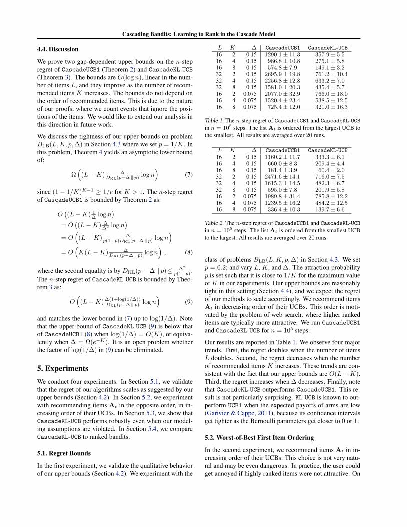
L K ∆ CascadeUCB1 CascadeKL-UCB16 2 0.15 1290.1 ± 11.3 357.9 ± 5.516 4 0.15 986.8 ± 10.8 275.1 ± 5.816 8 0.15 574.8 ± 7.9 149.1 ± 3.232 2 0.15 2695.9 ± 19.8 761.2 ± 10.432 4 0.15 2256.8 ± 12.8 633.2 ± 7.032 8 0.15 1581.0 ± 20.3 435.4 ± 5.716 2 0.075 2077.0 ± 32.9 766.0 ± 18.016 4 0.075 1520.4 ± 23.4 538.5 ± 12.516 8 0.075 725.4 ± 12.0 321.0 ± 16.3

Table 1. The n-step regret of CascadeUCB1 and CascadeKL-UCBin n = 105 steps. The list At is ordered from the largest UCB tothe smallest. All results are averaged over 20 runs.

L K ∆ CascadeUCB1 CascadeKL-UCB16 2 0.15 1160.2 ± 11.7 333.3 ± 6.116 4 0.15 660.0 ± 8.3 209.4 ± 4.416 8 0.15 181.4 ± 3.9 60.4 ± 2.032 2 0.15 2471.6 ± 14.1 716.0 ± 7.532 4 0.15 1615.3 ± 14.5 482.3 ± 6.732 8 0.15 595.0 ± 7.8 201.9 ± 5.816 2 0.075 1989.8 ± 31.4 785.8 ± 12.216 4 0.075 1239.5 ± 16.2 484.2 ± 12.516 8 0.075 336.4 ± 10.3 139.7 ± 6.6

Table 2. The n-step regret of CascadeUCB1 and CascadeKL-UCBin n = 105 steps. The list At is ordered from the smallest UCBto the largest. All results are averaged over 20 runs.

class of problems BLB(L,K, p,∆) in Section 4.3. We setp = 0.2; and vary L, K, and ∆. The attraction probabilityp is set such that it is close to 1/K for the maximum valueof K in our experiments. Our upper bounds are reasonablytight in this setting (Section 4.4), and we expect the regretof our methods to scale accordingly. We recommend itemsAt in decreasing order of their UCBs. This order is moti-vated by the problem of web search, where higher rankeditems are typically more attractive. We run CascadeUCB1

and CascadeKL-UCB for n = 105 steps.

Our results are reported in Table 1. We observe four majortrends. First, the regret doubles when the number of itemsL doubles. Second, the regret decreases when the numberof recommended items K increases. These trends are con-sistent with the fact that our upper bounds are O(L −K).Third, the regret increases when ∆ decreases. Finally, notethat CascadeKL-UCB outperforms CascadeUCB1. This re-sult is not particularly surprising. KL-UCB is known to out-perform UCB1 when the expected payoffs of arms are low(Garivier & Cappe, 2011), because its confidence intervalsget tighter as the Bernoulli parameters get closer to 0 or 1.

5.2. Worst-of-Best First Item Ordering

In the second experiment, we recommend items At in in-creasing order of their UCBs. This choice is not very natu-ral and may be even dangerous. In practice, the user couldget annoyed if highly ranked items were not attractive. On


the other hand, the user would provide a lot of feedback onlow quality items, which could speed up learning. We notethat the reward in our model does not depend on the orderof recommended items (Section 3.2). Therefore, the itemscan be ordered arbitrarily, perhaps to maximize feedback.In any case, we find it important to study the effect of thiscounterintuitive ordering, at least to demonstrate the effectof our modeling assumptions.

The experimental setup is the same as in Section 5.1. Ourresults are reported in Table 2. When compared to Table 1,the regret of CascadeUCB1 and CascadeKL-UCB decreasesfor all settings of K, L, and ∆; most prominently at largevalues of K. Our current analysis cannot explain this phe-nomenon and we leave it for future work.

5.3. Imperfect Model

The goal of this experiment is to evaluate CascadeKL-UCBin the setting where our modeling assumptions are not sat-isfied, to test its potential beyond our model. We generatedata from the dynamic Bayesian network (DBN) model ofChapelle & Zhang (2009), a popular extension of the cas-cade model which is parameterized by attraction probabil-ities ρ ∈ [0, 1]E , satisfaction probabilities ν ∈ [0, 1]E , andthe persistence of users γ ∈ (0, 1]. In the DBN model, theuser is recommended a list of K items A = (a1, . . . , aK)and examines it from the first recommended item a1 to thelast aK . After the user examines item ak, the item attractsthe user with probability ρ(ak). When the user is attractedby the item, the user clicks on it and is satisfied with prob-ability ν(ak). If the user is satisfied, the user does not ex-amine the remaining items. In any other case, the user ex-amines item ak+1 with probability γ. The reward is one ifthe user is satisfied with the list, and zero otherwise. Notethat this is not observed. The regret is defined accordingly.The feedback are clicks of the user. Note that the user canclick on multiple items.

The probability that at least one item in A = (a1, . . . , aK)is satisfactory is:

K∑k=1

γk−1w(ak)

k−1∏i=1

(1− w(ai)) ,

where w(e) = ρ(e)ν(e) is the probability that item e satis-fies the user after being examined. This objective is maxi-mized by the list of K items with largest weights w(e) thatare ordered in decreasing order of their weights. Note thatthe order matters.

The above objective is similar to that in cascading bandits(Section 3). Therefore, it may seem that our learning algo-rithms (Section 3.2) can also learn the optimal solution tothe DBN model. Unfortunately, this is not guaranteed. Thereason is that not all clicks of the user are satisfactory. Weillustrate this issue on a simple problem. Suppose that the

Step n20k 40k 60k 80k 100k

Reg

ret

0

200

400

600

800

1000

1200 = 1, (e) = 1 = 1, (e) = 0.7 = 0.7, (e) = 1 = 0.7, (e) = 0.7

Figure 1. The n-step regret of CascadeKL-UCB (solid lines) andRankedKL-UCB (dotted lines) in the DBN model in Section 5.3.

user clicks on multiple items. Then only the last click canbe satisfactory. But it does not have to be. For instance, itcould have happened that the user was unsatisfied with thelast click, and then scanned the recommended list until theend and left.

We experiment on the class of problems BLB(L,K, p,∆)in Section 4.3 and modify it as follows. The ground set Ehas L = 16 items and K = 4. The attraction probability ofitem e is ρ(e) = w(e), where w(e) is given in (6). We set∆ = 0.15. The satisfaction probabilities ν(e) of all itemsare the same. We experiment with two settings of ν(e), 1and 0.7; and with two settings of persistence γ, 1 and 0.7.We run CascadeKL-UCB for n = 105 steps and use the lastclick as an indicator that the user is satisfied with the item.

Our results are reported in Figure 1. We observe in all ex-periments that the regret of CascadeKL-UCB flattens. Thisindicates that CascadeKL-UCB learns the optimal solutionto the DBN model. An intuitive explanation for this resultis that the exact values of w(e) are not needed to performwell. Our current theory does not explain this phenomenonand we leave it for future work.

5.4. Ranked Bandits

In our final experiment, we compare CascadeKL-UCB to aranked bandit (Section 6) where the base bandit algorithmis KL-UCB. We refer to this method as RankedKL-UCB. Thechoice of the base algorithm is motivated by the followingreasons. First, KL-UCB is the best performing oracle in ourexperiments. Second, since both compared approaches usethe same oracle, the difference in their regrets is likely dueto their statistical efficiency, and not the oracle itself.

The experimental setup is the same as in Section 5.3. Ourresults are reported in Figure 1. We observe that the regretof RankedKL-UCB is significantly larger than the regret ofCascadeKL-UCB, about three times. The reason is that theregret in ranked bandits is Ω(K) (Section 6) and K = 4 in


this experiment. The regret of our algorithms is O(L−K)(Section 4.4). Note that CascadeKL-UCB is not guaranteedto be optimal in this experiment. Therefore, our results areencouraging and show that CascadeKL-UCB could be a vi-able alternative to more established approaches.

6. Related WorkRanked bandits are a popular approach in learning to rank(Radlinski et al., 2008) and they are closely related to ourwork. The key characteristic of ranked bandits is that eachposition in the recommended list is an independent banditproblem, which is solved by some base bandit algorithm.The solutions in ranked bandits are (1− 1/e) approximateand the regret is Ω(K) (Radlinski et al., 2008), where K isthe number of recommended items. Cascading bandits canbe viewed as a form of ranked bandits where each recom-mended item attracts the user independently. We proposenovel algorithms for this setting that can learn the optimalsolution and whose regret decreases with K. We compareone of our algorithms to ranked bandits in Section 5.4.

Our learning problem is of a combinatorial nature, our ob-jective is to learn K most attractive items out of L. In thissense, our work is related to stochastic combinatorial ban-dits, which are often studied with linear rewards and semi-bandit feedback (Gai et al., 2012; Kveton et al., 2014a;b;2015). The key differences in our work are that the rewardfunction is non-linear in unknown parameters; and that thefeedback is less than semi-bandit, only a subset of the rec-ommended items is observed.

Our reward function is non-linear in unknown parameters.These types of problems have been studied before in vari-ous contexts. Filippi et al. (2010) proposed and analyzed ageneralized linear bandit with bandit feedback. Chen et al.(2013) studied a variant of stochastic combinatorial semi-bandits whose reward function is a known monotone func-tion of a linear function in unknown parameters. Le et al.(2014) studied a network optimization problem whose re-ward function is a non-linear function of observations.

Bartok et al. (2012) studied finite partial monitoring prob-lems. This is a very general class of problems with finitelymany actions, which are chosen by the learning agent; andfinitely many outcomes, which are determined by the envi-ronment. The outcome is unobserved and must be inferredfrom the feedback of the environment. Cascading banditscan be viewed as finite partial monitoring problems wherethe actions are lists of K items out of L and the outcomesare the corners of a L-dimensional binary hypercube. Bar-tok et al. (2012) proposed an algorithm that can solve suchproblems. This algorithm is computationally inefficient inour problem because it needs to reason over all pairs of ac-tions and stores vectors of length 2L. Bartok et al. (2012)also do not prove logarithmic distribution-dependent regret

bounds as in our work.

Agrawal et al. (1989) studied a partial monitoring problemwith non-linear rewards. In this problem, the environmentdraws a state from a distribution that depends on the actionof the learning agent and an unknown parameter. The formof this dependency is known. The state of the environmentis observed and determines reward. The reward is a knownfunction of the state and action. Agrawal et al. (1989) alsoproposed an algorithm for their problem and proved a log-arithmic distribution-dependent regret bound. Similarly toBartok et al. (2012), this algorithm is computationally in-efficient in our setting.

Lin et al. (2014) studied partial monitoring in combinato-rial bandits. The setting of this work is different from ours.Lin et al. (2014) assume that the feedback is a linear func-tion of the weights of the items that is indexed by actions.Our feedback is a non-linear function of the weights of theitems.

Mannor & Shamir (2011) and Caron et al. (2012) studied anopposite setting to ours, where the learning agent observesa superset of chosen items. Chen et al. (2014) studied thisproblem in stochastic combinatorial semi-bandits.

7. ConclusionsIn this paper, we propose a learning variant of the cascademodel (Craswell et al., 2008), a popular model of user be-havior in web search. We propose two algorithms for solv-ing it, CascadeUCB1 and CascadeKL-UCB, and prove gap-dependent upper bounds on their regret. Our analysis ad-dresses two main challenges of our problem, a non-linearreward function and limited feedback. We evaluate our al-gorithms on several problems and show that they performwell even when our modeling assumptions are violated.

We leave open several questions of interest. For instance,we show in Section 5.3 that CascadeKL-UCB can learn theoptimal solution to the DBN model. This indicates that theDBN model is learnable in the bandit setting and we leavethis for future work. Note that the regret in cascading ban-dits is Ω(L) (Section 4.3). Therefore, our learning frame-work is not practical when the number of items L is large.Similarly to Slivkins et al. (2013), we plan to address thisissue by embedding the items in some feature space, alongthe lines of Wen et al. (2015). Finally, we want to general-ize our results to more complex problems, such as learningrouting paths in computer networks where the connectionsfail with unknown probabilities.

From the theoretical point of view, we would like to closethe gap between our upper and lower bounds. In addition,we want to derive gap-free bounds. Finally, we would liketo refine our analysis so that it explains that the reverse or-dering of recommended items yields smaller regret.


ReferencesAgichtein, Eugene, Brill, Eric, and Dumais, Susan. Im-

proving web search ranking by incorporating user be-havior information. In Proceedings of the 29th AnnualInternational ACM SIGIR Conference, pp. 19–26, 2006.

Agrawal, Rajeev, Teneketzis, Demosthenis, and Anan-tharam, Venkatachalam. Asymptotically efficient adap-tive allocation schemes for controlled i.i.d. processes:Finite parameter space. IEEE Transactions on AutomaticControl, 34(3):258–267, 1989.

Auer, Peter, Cesa-Bianchi, Nicolo, and Fischer, Paul.Finite-time analysis of the multiarmed bandit problem.Machine Learning, 47:235–256, 2002.

Bartok, Gabor, Zolghadr, Navid, and Szepesvari, Csaba.An adaptive algorithm for finite stochastic partial moni-toring. In Proceedings of the 29th International Confer-ence on Machine Learning, 2012.

Becker, Hila, Meek, Christopher, and Chickering,David Maxwell. Modeling contextual factors of clickrates. In Proceedings of the 22nd AAAI Conference onArtificial Intelligence, pp. 1310–1315, 2007.

Boucheron, Stephane, Lugosi, Gabor, and Massart, Pascal.Concentration Inequalities: A Nonasymptotic Theory ofIndependence. Oxford University Press, 2013.

Caron, Stephane, Kveton, Branislav, Lelarge, Marc, andBhagat, Smriti. Leveraging side observations in stochas-tic bandits. In Proceedings of the 28th Conference onUncertainty in Artificial Intelligence, pp. 142–151, 2012.

Chapelle, Olivier and Zhang, Ya. A dynamic bayesian net-work click model for web search ranking. In Proceed-ings of the 18th International Conference on World WideWeb, pp. 1–10, 2009.

Chen, Wei, Wang, Yajun, and Yuan, Yang. Combinato-rial multi-armed bandit: General framework, results andapplications. In Proceedings of the 30th InternationalConference on Machine Learning, pp. 151–159, 2013.

Chen, Wei, Wang, Yajun, and Yuan, Yang. Combinatorialmulti-armed bandit and its extension to probabilisticallytriggered arms. CoRR, abs/1407.8339, 2014.

Craswell, Nick, Zoeter, Onno, Taylor, Michael, and Ram-sey, Bill. An experimental comparison of click position-bias models. In Proceedings of the 1st ACM Interna-tional Conference on Web Search and Data Mining, pp.87–94, 2008.

Filippi, Sarah, Cappe, Olivier, Garivier, Aurelien, andSzepesvari, Csaba. Parametric bandits: The generalizedlinear case. In Advances in Neural Information Process-ing Systems 23, pp. 586–594, 2010.

Gai, Yi, Krishnamachari, Bhaskar, and Jain, Rahul. Com-binatorial network optimization with unknown variables:Multi-armed bandits with linear rewards and individualobservations. IEEE/ACM Transactions on Networking,20(5):1466–1478, 2012.

Garivier, Aurelien and Cappe, Olivier. The KL-UCB al-gorithm for bounded stochastic bandits and beyond. InProceeding of the 24th Annual Conference on LearningTheory, pp. 359–376, 2011.

Guo, Fan, Liu, Chao, Kannan, Anitha, Minka, Tom, Taylor,Michael, Wang, Yi Min, and Faloutsos, Christos. Clickchain model in web search. In Proceedings of the 18thInternational Conference on World Wide Web, pp. 11–20, 2009a.

Guo, Fan, Liu, Chao, and Wang, Yi Min. Efficient multiple-click models in web search. In Proceedings of the 2ndACM International Conference on Web Search and DataMining, pp. 124–131, 2009b.

Kveton, Branislav, Wen, Zheng, Ashkan, Azin, Eydgahi,Hoda, and Eriksson, Brian. Matroid bandits: Fast com-binatorial optimization with learning. In Proceedings ofthe 30th Conference on Uncertainty in Artificial Intelli-gence, pp. 420–429, 2014a.

Kveton, Branislav, Wen, Zheng, Ashkan, Azin, and Valko,Michal. Learning to act greedily: Polymatroid semi-bandits. CoRR, abs/1405.7752, 2014b.

Kveton, Branislav, Wen, Zheng, Ashkan, Azin, andSzepesvari, Csaba. Tight regret bounds for stochasticcombinatorial semi-bandits. In Proceedings of the 18thInternational Conference on Artificial Intelligence andStatistics, 2015.

Lai, T. L. and Robbins, Herbert. Asymptotically efficientadaptive allocation rules. Advances in Applied Mathe-matics, 6(1):4–22, 1985.

Le, Thanh, Szepesvari, Csaba, and Zheng, Rong. Sequen-tial learning for multi-channel wireless network monitor-ing with channel switching costs. IEEE Transactions onSignal Processing, 62(22):5919–5929, 2014.

Lin, Tian, Abrahao, Bruno, Kleinberg, Robert, Lui, John,and Chen, Wei. Combinatorial partial monitoring gamewith linear feedback and its applications. In Proceedingsof the 31st International Conference on Machine Learn-ing, pp. 901–909, 2014.

Mannor, Shie and Shamir, Ohad. From bandits to experts:On the value of side-observations. In Advances in NeuralInformation Processing Systems 24, pp. 684–692, 2011.


Radlinski, Filip and Joachims, Thorsten. Query chains:Learning to rank from implicit feedback. In Proceedingsof the 11th ACM SIGKDD International Conference onKnowledge Discovery and Data Mining, pp. 239–248,2005.

Radlinski, Filip, Kleinberg, Robert, and Joachims,Thorsten. Learning diverse rankings with multi-armedbandits. In Proceedings of the 25th International Con-ference on Machine Learning, pp. 784–791, 2008.

Richardson, Matthew, Dominowska, Ewa, and Ragno,Robert. Predicting clicks: Estimating the click-throughrate for new ads. In Proceedings of the 16th InternationalConference on World Wide Web, pp. 521–530, 2007.

Slivkins, Aleksandrs, Radlinski, Filip, and Gollapudi,Sreenivas. Ranked bandits in metric spaces: Learning di-verse rankings over large document collections. Journalof Machine Learning Research, 14(1):399–436, 2013.

Wen, Zheng, Kveton, Branislav, and Ashkan, Azin. Effi-cient learning in large-scale combinatorial semi-bandits.In Proceedings of the 32nd International Conference onMachine Learning, 2015.


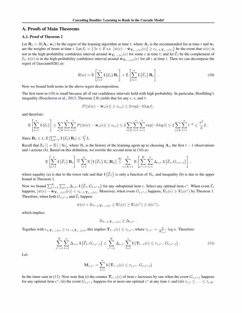
A. Proofs of Main TheoremsA.1. Proof of Theorem 2

Let Rt = R(At,wt) be the regret of the learning algorithm at time t, where At is the recommended list at time t and wt

are the weights of items at time t. Let Et =∃e ∈ E s.t.

∣∣w(e)− wTt−1(e)(e)∣∣ ≥ ct−1,Tt−1(e)

be the event that w(e) is

not in the high-probability confidence interval around wTt−1(e)(e) for some e at time t; and let Et be the complement ofEt, w(e) is in the high-probability confidence interval around wTt−1(e)(e) for all e at time t. Then we can decompose theregret of CascadeUCB1 as:

R(n) = E

[n∑t=1

1EtRt

]+ E

[n∑t=1

1EtRt

]. (10)

Now we bound both terms in the above regret decomposition.

The first term in (10) is small because all of our confidence intervals hold with high probability. In particular, Hoeffding’sinequality (Boucheron et al., 2013, Theorem 2.8) yields that for any e, s, and t:

P (|w(e)− ws(e)| ≥ ct,s) ≤ 2 exp[−3 log t] ,

and therefore:

E

[n∑t=1

1Et

]≤∑e∈E

n∑t=1

t∑s=1

P (|w(e)− ws(e)| ≥ ct,s) ≤ 2∑e∈E

n∑t=1

t∑s=1

exp[−3 log t] ≤ 2∑e∈E

n∑t=1

t−2 ≤ π2

3L .

Since Rt ≤ 1, E [∑nt=1 1EtRt] ≤ π2

3 L.

Recall that Et [·] = E [· |Ht], where Ht is the history of the learning agent up to choosing At, the first t− 1 observationsand t actions (4). Based on this definition, we rewrite the second term in (10) as:

E

[n∑t=1

1EtRt

](a)=

n∑t=1

E[1EtEt [Rt]

] (b)≤

L∑e=K+1

E

[K∑

e∗=1

n∑t=1

∆e,e∗1Et, Ge,e∗,t

],

where equality (a) is due to the tower rule and that 1Et

is only a function of Ht, and inequality (b) is due to the upperbound in Theorem 1.

Now we bound∑Ke∗=1

∑nt=1 ∆e,e∗1

Et, Ge,e∗,t

for any suboptimal item e. Select any optimal item e∗. When event Et

happens,∣∣w(e)− wTt−1(e)(e)

∣∣ < ct−1,Tt−1(e). Moreover, when event Ge,e∗,t happens, Ut(e) ≥ Ut(e∗) by Theorem 1.

Therefore, when both Ge,e∗,t and Et happen:

w(e) + 2ct−1,Tt−1(e) ≥ Ut(e) ≥ Ut(e∗) ≥ w(e∗) ,

which implies:

2ct−1,Tt−1(e) ≥ ∆e,e∗ .

Together with cn,Tt−1(e) ≥ ct−1,Tt−1(e), this implies Tt−1(e) ≤ τe,e∗ , where τe,e∗ = 6∆2e,e∗

log n. Therefore:

K∑e∗=1

n∑t=1


≤

K∑e∗=1

∆e,e∗

n∑t=1

1Tt−1(e) ≤ τe,e∗ , Ge,e∗,t . (11)

Let:

Me,e∗ =

n∑t=1

1Tt−1(e) ≤ τe,e∗ , Ge,e∗,t

be the inner sum in (11). Now note that (i) the counter Tt−1(e) of item e increases by one when the event Ge,e∗,t happensfor any optimal item e∗, (ii) the event Ge,e∗,t happens for at most one optimal e∗ at any time t; and (iii) τe,1 ≤ . . . ≤ τe,K .


Based on these facts, it follows that Me,e∗ ≤ τe,e∗ , and moreover∑Ke∗=1 Me,e∗ ≤ τe,K . Therefore, the right-hand side of

(11) can be bounded from above by:

max

K∑

e∗=1

∆e,e∗me,e∗ : 0 ≤ me,e∗ ≤ τe,e∗ ,K∑

e∗=1

me,e∗ ≤ τe,K

.

Since the gaps are decreasing, ∆e,1 ≥ . . . ≥ ∆e,K , the solution to the above problem is m∗e,1 = τe,1, m∗e,2 = τe,2 − τe,1,. . . , m∗e,K = τe,K − τe,K−1. Therefore, the value of (11) is bounded from above by:[

∆e,11

∆2e,1

+

K∑e∗=2

∆e,e∗

(1

∆2e,e∗− 1

∆2e,e∗−1

)]6 log n .

By Lemma 3 of Kveton et al. (2014a), the above term is bounded by 12∆e,K

log n. Finally, we chain all inequalities and sumover all suboptimal items e.

A.2. Proof of Theorem 3

Let Rt = R(At,wt) be the regret of the learning algorithm at time t, where At is the recommended list at time t and wt

are the weights of items at time t. Let Et = ∃1 ≤ e ≤ K s.t. w(e) > Ut(e) be the event that the attraction probabilityof at least one optimal item is above its upper confidence bound at time t. Let Et be the complement of event Et. Then wecan decompose the regret of CascadeKL-UCB as:

R(n) = E

[n∑t=1

1EtRt

]+ E

[n∑t=1

1EtRt

]. (12)

By Theorems 2 and 10 of Garivier & Cappe (2011), thanks to the choice of the upper confidence bound Ut, the first termin (12) is bounded as E [

∑nt=1 1EtRt] ≤ 7K log log n. As in the proof of Theorem 2, we rewrite the second term as:

E

[n∑t=1

1EtRt

]=

n∑t=1

E[1EtEt [Rt]

]≤

L∑e=K+1

E

[K∑

e∗=1

n∑t=1


].

Now note that for any suboptimal item e and τe,e∗ > 0:

E

[K∑

e∗=1

n∑t=1


]≤ E

[K∑

e∗=1

n∑t=1

∆e,e∗1Tt−1(e) ≤ τe,e∗ , Ge,e∗,t

]+ (13)

K∑e∗=1

∆e,e∗E

[n∑t=1

1Tt−1(e) > τe,e∗ , Et, Ge,e∗,t

].

Let:

τe,e∗ =1 + ε

DKL(w(e) ‖ w(e∗))(log n+ 3 log log n) .

Then by the same argument as in Theorem 2 and Lemma 8 of Garivier & Cappe (2011):

E

[n∑t=1

1Tt−1(e) > τe,e∗ , Et, Ge,e∗,t

]≤ C2(ε)

nβ(ε)

holds for any suboptimal e and optimal e∗. So the second term in (13) is bounded from above by K C2(ε)nβ(ε)

. Now we boundthe first term in (13). By the same argument as in the proof of Theorem 2:

K∑e∗=1

n∑t=1

∆e,e∗1Tt−1(e) ≤ τe,e∗ , Ge,e∗,t ≤[∆e,1

DKL(w(e) ‖ w(1))+

K∑e∗=2

∆e,e∗

(1

DKL(w(e) ‖ w(e∗))− 1

DKL(w(e) ‖ w(e∗ − 1))

)](1 + ε)(log n+ 3 log log n)


holds for any suboptimal item e. By Lemma 2, the leading constant is bounded as:

∆e,1

DKL(w(e) ‖ w(1))+

K∑e∗=2

∆e,e∗

(1

DKL(w(e) ‖ w(e∗))− 1

DKL(w(e) ‖ w(e∗ − 1))

)≤ ∆e,K(1 + log(1/∆e,K))

DKL(w(e) ‖ w(K)).

Finally, we chain all inequalities and sum over all suboptimal items e.

B. Technical LemmasLemma 1. Let A = (a1, . . . , aK) and B = (b1, . . . , bK) be any two lists of K items from ΠK(E) such that ai = bj onlyif i = j. Let w ∼ P in Assumption 1. Then:

E

[K∏k=1

w(ak)−K∏k=1

w(bk)

]=

K∑k=1

E

[k−1∏i=1

w(ai)

]E [w(ak)−w(bk)]

K∏j=k+1

E [w(bj)]

.

Proof. First, we prove that:

K∏k=1

w(ak)−K∏k=1

w(bk) =

K∑k=1

(k−1∏i=1

w(ai)

)(w(ak)− w(bk))

K∏j=k+1

w(bj)

holds for any w ∈ 0, 1L. The proof is by induction on K. The claim holds obviously for K = 1. Now suppose that theclaim holds for any A,B ∈ ΠK−1(E). Let A,B ∈ ΠK(E). Then:

K∏k=1

w(ak)−K∏k=1

w(bk) =

K∏k=1

w(ak)− w(bK)

K−1∏k=1

w(ak) + w(bK)

K−1∏k=1

w(ak)−K∏k=1

w(bk)

= (w(aK)− w(bK))

K−1∏k=1

w(ak) + w(bK)

[K−1∏k=1

w(ak)−K−1∏k=1

w(bk)

]

= (w(aK)− w(bK))

K−1∏k=1

w(ak) +

K−1∑k=1

(k−1∏i=1

w(ai)

)(w(ak)− w(bk))

K∏j=k+1

w(bj)

=

K∑k=1

(k−1∏i=1

w(ai)

)(w(ak)− w(bk))

K∏j=k+1

w(bj)

.

The third equality is by our induction hypothesis. Finally, note that w is drawn from a factored distribution. Therefore, wecan decompose the expectation of the product as a product of expectations, and our claim follows.

Lemma 2. Let p1 ≥ . . . ≥ pK > p be K + 1 probabilities and ∆k = pk − p for 1 ≤ k ≤ K. Then:

∆1

DKL(p ‖ p1)+

K∑k=2

∆k

(1

DKL(p ‖ pk)− 1

DKL(p ‖ pk−1)

)≤ ∆K(1 + log(1/∆K))

DKL(p ‖ pK).

Proof. First, we note that:

∆1

DKL(p ‖ p1)+

K∑k=2

∆k

(1

DKL(p ‖ pk)− 1

DKL(p ‖ pk−1)

)=

K−1∑k=1

∆k −∆k+1

DKL(p ‖ pk)+

∆K

DKL(p ‖ pK).

The summation over k can be bounded from above by a definite integral:

K−1∑k=1

∆k −∆k+1

DKL(p ‖ pk)=

K−1∑k=1

∆k −∆k+1

DKL(p ‖ p+ ∆k)≤∫ ∆1

∆K

1

DKL(p ‖ p+ x)dx ≤

∫ 1

∆K

1

DKL(p ‖ p+ x)dx ,


where the first inequality follows from the fact that 1/DKL(p ‖ p + x) decreases on x ≥ 0. To the best of our knowledge,the integral of 1/DKL(p ‖ p+ x) over x does not have a simple analytic solution. Therefore, we integrate an upper boundon 1/DKL(p ‖ p+ x) which does. In particular, note that for any x ≥ ∆K :

DKL(p ‖ p+ x) ≥ DKL(p ‖ p+ ∆K)

∆Kx =

DKL(p ‖ pK)

∆Kx

because DKL(p ‖ p+ x) is convex, increasing in x ≥ 0, and its minimum is attained at x = 0. Therefore:∫ 1

∆K

1

DKL(p ‖ p+ x)dx ≤ ∆K

DKL(p ‖ pK)

∫ 1

∆K

1

xdx =

∆K

DKL(p ‖ pK)log(1/∆K) .

Finally, we chain all inequalities and get the final result.

cascading bandits: learning to rank in the cascade model · cascading bandits: learning to rank in...

Documents