cartesian differential categories

Theory and Applications of Categories, Vol. 22, No. 23, 2009, pp. 622–672.

CARTESIAN DIFFERENTIAL CATEGORIES

R.F. BLUTE, J.R.B. COCKETT AND R.A.G. SEELY

Abstract. This paper revisits the authors’ notion of a differential category from adifferent perspective. A differential category is an additive symmetric monoidal categorywith a comonad (a “coalgebra modality”) and a differential combinator. The morphismsof a differential category should be thought of as the linear maps; the differentiable orsmooth maps would then be morphisms of the coKleisli category. The purpose of thepresent paper is to directly axiomatize differentiable maps and thus to move the emphasisfrom the linear notion to structures resembling the coKleisli category. The result is asetting with a more evident and intuitive relationship to the familiar notion of calculuson smooth maps. Indeed a primary example is the category whose objects are Euclideanspaces and whose morphisms are smooth maps.

A Cartesian differential category is a Cartesian left additive category which possesses aCartesian differential operator. The differential operator itself must satisfy a number ofequations, which guarantee, in particular, that the differential of any map is “linear” ina suitable sense.

We present an analysis of the basic properties of Cartesian differential categories. Weshow that under modest and natural assumptions, the coKleisli category of a differentialcategory is Cartesian differential. Finally we present a (sound and complete) termcalculus for these categories which allows their structure to be analysed using essentiallythe same language one might use for traditional multi-variable calculus.

0. Introduction

Over the past few centuries, one of the most fundamental concepts in all of mathematicshas been differentiation. In recent decades several attempts have been made to abstractthis notion, including approaches based on geometric, algebraic, and logical intuitions.The approach of the current paper is categorical, insofar as we wish to consider axiom-atizations of categories which have sufficient structure to define differentiation of maps.Any additional categorical structure, e.g. monoidal, Cartesian, or comonadic, exists insupport of differentiation.

In [BCS 06], the current authors introduced the notion of a differential category toprovide a basic axiomatization for differential operators in monoidal categories. Theinitial impetus for the definition came from work of Ehrhard and Regnier [Ehrhard &Regnier 05, Ehrhard & Regnier 03], who defined first a notion of differential λ-calculus

Received by the editors 2008-11-29 and, in revised form, 2009-12-08.Transmitted by Robert Pare. Published on 2009-12-10.2000 Mathematics Subject Classification: 18D10,18C20,12H05,32W99.Key words and phrases: monoidal categories, differential categories, Kleisli categories, differential

operators.c© R.F. Blute, J.R.B. Cockett and R.A.G. Seely, 2009. Permission to copy for private use granted.

622

CARTESIAN DIFFERENTIAL CATEGORIES 623

and subsequently differential proof nets. The differential λ-calculus is an extension ofsimply-typed λ-calculus with an additional operation allowing the differentiation of terms.Differential proof nets are a (graph-theoretic) syntax for linear logic extended with adifferential operator on proofs. An important feature of their systems, not precluded inours, is that in one setting, they combine the essence of both calculus and computability.

Their work grew out of the development of models of linear logic (examples of ∗-autonomous categories) in which there was a natural differential operator, such as Kothespaces [Ehrhard 01]. Every model of linear logic comes equipped with a monad, the storageoperator, from which the coKleisli category arises. One can then abstract away frommodels of linear logic, retaining the comonad as the key feature. From this perspectiveit is a very natural step to consider the coKleisli categories of such models, not leastbecause it is this setting which supports a calculus which much more closely resemblesthe elementary differential calculus with which we are all familiar. The calculus oneobtains from this perspective is quite different than the differential lambda-calculus ofEhrhard and Regnier, in that it is directly inspired by the coKleisli structure. And so thisleft open the question of how to characterize this situation.

The notion of a differential category provides a basic axiomatization for differentialoperators in monoidal categories, which not only generalizes the work of Ehrhard andRegnier but also captures the standard elementary models of differential calculus andprovides a theoretical substrate for studying a number of less standard examples. Thestructure necessary to support differentiation in [BCS 06] is an additive, monoidal categorywith a coalgebra modality. (These terms will be reviewed below.) The morphisms in adifferential category should be thought of as linear maps, with maps in the coKleislicategory being the smooth maps. Then the differential operator is of the following type:

f :SA // B

D⊗[f ]:A⊗ SA // B

One then writes down suitable axioms which such an operator must satisfy. In particular,we have the Leibniz rule, the chain rule, and other basic rules of differentiation expressedcoalgebraically.

The goal of the present paper is to develop an axiomatisation which directly character-izes the smooth maps: in other words, to characterize the coKleisli structure of differentialcategories directly. This leads us to the notion of a Cartesian differential category. Thisnotion embodies the multi-variable differential calculus which, being a fundamental tool ofmodern mathematics, is well worth studying in its own right. The basic structure neededfor Cartesian differential categories is simpler than is needed for differential categories:just a left additive category with finite products. The differential operator takes on thefollowing form

Xf // Y

X ×XD×[f ]

// Y

However the necessary equations turn out to be more complicated, and the passagefrom the coKleisli category of a differential category to a Cartesian differential category

624 R.F. BLUTE, J.R.B. COCKETT AND R.A.G. SEELY

turns out to be surprisingly subtle. While we do describe the conditions under which adifferential category gives rise to a Cartesian differential category as its coKleisli category,a full characterization of this situation is left to a sequel. The main result in this directionis Proposition 3.2.1.

The organization of the paper is as follows. Fundamental to differentiation is theability to add maps: however, the settings in which we are interested are not additivelyenriched. Therefore the first section is dedicated developing the general theory of leftadditive categories. In the second section we introduce the key notion of a Cartesiandifferential operator and the equations it satisfies. In this section, we also show how mostof the axiomatization of these categories is determined by requiring that their “bundlecategories” behave in the expected manner. These are fibrations which carry the differ-ential structure, insofar as the composition of maps is just the chain rule. It is possible todevelop higher-order bundle categories in which composition is determined by the higher-order (Faa di Bruno) chain rules. These higher-differential bundle categories completelydetermine all the axiomatization of Cartesian differential categories, but developing thiswould require more technical apparatus than seems justified in this paper, so will bepresented elsewhere.

As always, we are interested in graphical representations of morphisms in free cate-gories, an approach begun in [BCST 97]. But in this paper we focus more on a termcalculus. This calculus can be seen as effectively reimagining the traditional differentialcalculus as a rewrite system. Section 4 of this paper is devoted to analyzing this systemin detail. In particular, we show the system’s soundness and completeness. The termcalculus allows for an elegant description of free Cartesian differential categories, whichwe shall present in a sequel.

The reader should keep one key simple example in mind when reading the paper: thecategory of smooth maps, which behaves just as one would expect from a first year calculuscourse. Objects are natural numbers and maps n // m are smooth maps IRn // IRm.

It is easiest to describe the differential operator via an example. Suppose we have asmooth map f : 3 // 1, such as f(x, y, z) = xyz. The Jacobian of this map is [yz, xz, xy]which may be regarded as a smooth operator which assigns a linear operator to any point(x, y, z). This is how we get a smooth map D×(f): IR3 × IR3 // IR, which is linear in thefirst variable (in the first triple of coordinates):

D×(f): ((u, v, w), (r, s, t)) 7→ (st, rt, rs) · (u, v, w) = stu+ rtv + rsw

In fact, the notation we will introduce in our term calculus is slightly different thanthis, and keeps more careful track of free vs. bound variables. This leads to one ofour axioms for Cartesian differential categories: the function D[f ] is linear in its first nvariables. The rest of the axioms express other aspects of differentiability.

The foundations for differential calculus may be approached in at least three funda-mentally different ways. At one extreme is the synthetic approach where one wishes tocreate a calculus so deeply embedded into the underlying set theory that one is willing to


turn the world of mathematics and philosophy upside down to ensure that everything be-comes differentiable. Somewhere nearer the middle is the Platonic approach which takesthe view that the ability to differentiate ultimately devolves onto the topological and lim-iting properties of a single crucial object: the real line. And then there is the mechanicalapproach. Devoid of overarching philosophy or greater purpose, it takes calculus as asystem which, like any other, should immediately be taken apart to determine how thebehavior of one part depends on structure in some other part. Dismembering calculus inthis manner, it seeks to reuse these structures in outlandish configurations elsewhere.

This work belongs unapologetically to this last camp. It seeks to isolate some basicstructural properties which give rise to behaviors reminiscent of the differential calculus.We believe abstracting differential calculus in this manner serves a useful purpose whichalso reflects developments in other areas. Differentials (over arbitrary base rings) areused non-trivially in various areas of algebraic geometry, and differentials also appearin different guises in both combinatorics and computer science. A framework unifyingsuch notions is useful, and in particular allows one to distinguish clearly between what isgeneric and what is specific.

1. Left additive categories

The purpose of this section is to develop the basic theory of left additive categories whichunderlies the theory of Cartesian differential categories. As a basic example consider thecategory of commutative monoids with morphisms which are arbitrary maps which ignorethe additive structure. Despite the fact that additive structure is being ignored, the mapsbetween any two objects have a natural additive structure, given by pointwise addition(f+g)(x) = f(x)+g(x). Furthermore, this additive structure is preserved by compositionon the left h(f + g) = hf + hg (throughout the paper we use the diagrammatic orderof composition, sometimes denoted with a semicolon, often just by juxtaposition). Acategory with the property that each homset is a commutative monoid and for whichcomposition on the left preserves this structure is called a left additive category.

This category may be viewed rather differently: it is the coKleisli category with respectto the comonad generated from the comonad on commutative monoids generated by thecomposite of the underlying functor and the free functor. This illustrates an importantway in which left additive structure arises: any (non-additive) comonad on an additive(or indeed left-additive) category always has its coKleisli category left-additive.

Another basic example of a left additive category which is central to this paper consistsof the category whose objects are finite dimensional real vector spaces and whose mapsare (infinitely) differentiable maps. These maps allow pointwise addition and so certainlyform a left additive category. In addition, this category has a differential structure whichis the main subject matter of the paper and is discussed in the next section.

1.1. The basic definition.


1.1.1. Definition. A category X is left additive1 in case each hom-set is a commu-tative monoid and f(g+h) = (fg)+(fh) and f0 = 0. A map h in a left additive categoryis said to be additive if it also preserves the additive structure of the hom-set on the right(f + g)h = (fh) + (gh) and 0h = 0.

In general additive maps will be the exception in a left additive category. However,the additive maps form an interesting subcategory:

1.1.2. Proposition. In any left additive category,

1. 0 maps are additive;

2. additive maps are closed under addition;

3. additive maps are closed under composition;

4. all identity maps are additive;

5. if m is an additive monic and fm is additive then f is additive;

6. if g is a retraction which is additive and the composite gh is additive then h isadditive;

7. if r is a retraction with section m so that the idempotent rm is additive, then r isadditive iff its section m is additive;

8. if f is an isomorphism which is additive, then f−1 is additive.

Proof. (1): (f + g)0 = 0 = 0 + 0 = f0 + g0.(2): If f and g are additive then (x+y)(f+g) = (x+y)f+(x+y)g = xf+yf+xg+yg =

x(f + g) + y(f + g).(3): If f and g are additive then (x+ y)fg = (xf + yf)g = xfg + yfg.(4 ,5): Immediate.(6): This is slightly more subtle: suppose g is additive and a retraction, so that there

is a g′ with g′g = 1, and gh is additive then, as (x+y) = (xg′g+yg′g) = (xg′+yg′)g then

(x+ y)h = (xg′ + yg′)gh = xg′gh+ yg′gh = xh+ yh.

(7): Since rm is additive, by (5) if m is additive, then r is additive; and by (6) if r isadditive then m is additive.

(8): If f is an isomorphism it is certainly a retraction and 1 = ff−1 is certainlyadditive so by the previous property f−1 is additive.

1We should emphasize that our “additive categories” are commutative monoid enriched categories,rather than Abelian group enriched; some people might prefer to call them “semi-additive”. Furthermore,we do not require biproducts as part of the structure at this stage. In particular, our definition is notthe same as the one in [[M 71]].


Note that it is certainly not the case that all isomorphisms are additive. However, wecan conclude:

1.1.3. Corollary. The additive maps of a left additive category X form an additivesubcategory whose inclusion I: X+

// X reflects isomorphisms.

1.1.4. Example. The category CMon of commutative monoids with “set maps” (i.e.without any preservation properties) is left additive, but generally its maps are not addi-tive. Left additivity is easily shown:

f(g + h)(x) = (g + h)(f(x)) = g(f(x)) + h(f(x)) = (fg)(x) + (fh)(x) = (fg + fh)(x)

(and 0 is similar). As an example of the failure of additivity, however, consider that(0f)(x) = f(0(x)) = f(0), and we have explicitly not required f(0) = 0 (and similarly foraddition). The additive maps in this setting are just the commutative monoid homomor-phisms.

1.2. Cartesian left additive categories. Our main interest centres around leftadditive categories which have products which behave coherently with respect to theadditive structure:

1.2.1. Definition. A Cartesian left additive category is a left additive categorywith products such that the structure maps π0, π1, and ∆ are additive and that wheneverf and g are additive then f × g is additive.

Notice that if f and g are additive then 〈f, g〉 is additive as

(x+ y)〈f, g〉 = (x+ y)∆(f × g) = x∆(f × g) + y∆(f × g) = x〈f, g〉+ y〈f, g〉

Conversely one may replace the requirement that ∆ is additive and that × preservesadditivity by the single requirement that pairing preserves additivity as both can be ex-pressed by pairing additive maps. Thus, equivalently, a category is Cartesian left additivein case it has products for which the projections are additive and whenever f and g areadditive then 〈f, g〉 is additive. Cartesian left additive categories can be formulated invarious other ways as well:

1.2.2. Proposition. The following are equivalent:

(i) A Cartesian left additive category;

(ii) A left additive category with products such that all projections and pairings of additivemaps are additive.

(iii) A left additive category for which X+ has biproducts and the the inclusion I: X+//X

creates products;

(iv) A Cartesian category X in which each object is equipped with a chosen commutativemonoid structure compatible with products: (+A:A×A //A, 0A: 1 //A) satisfying+A×B = 〈(π0 × π0)+A, (π1 × π1)+B〉 and 0A×B = 〈0A, 0B〉.


Proof.

(i) ⇔ (ii) Above.

(ii) ⇒ (iii) Clearly as the product structure is additive the category of additive mapswill have products (and so biproducts). Further, the inclusion functor will clearlycreate products.

(iii) ⇒ (iv) Define +A = π0 + π1 and 0A = 0 then this gives each object an additivestructure. Note that

+A×B = π0 + π1 = (π0 + π1)〈π0, π1〉= 〈π0π0 + π1π0, π0π1 + π1π1〉= 〈(π0 × π0)+A, (π1 × π1)+B〉

(iv) ⇒ (i) Define f + g = 〈f, g〉+B then this certainly makes the category left additive.Furthermore, each πi is additive as

(〈f, f ′〉+ 〈g, g′〉)π0 = 〈〈f, f ′〉, 〈g, g′〉〉(π0 × π0)+ = 〈f, f ′〉π0 + 〈g, g′〉π0.

Clearly maps are additive in case they are homomorphisms of the chosen additivestructure: but this means if f and g are additive then 〈f, g〉 is additive as theadditive structure on the product is the product additive structure!

The last characterization does rely on the choice of product structure. The equivalenceto being Cartesian left additive informs us that the choice can be made up to additiveisomorphism. For, seen as a left additive category, there is one global structure albeit itmay be represented locally in a variety of coherent ways.

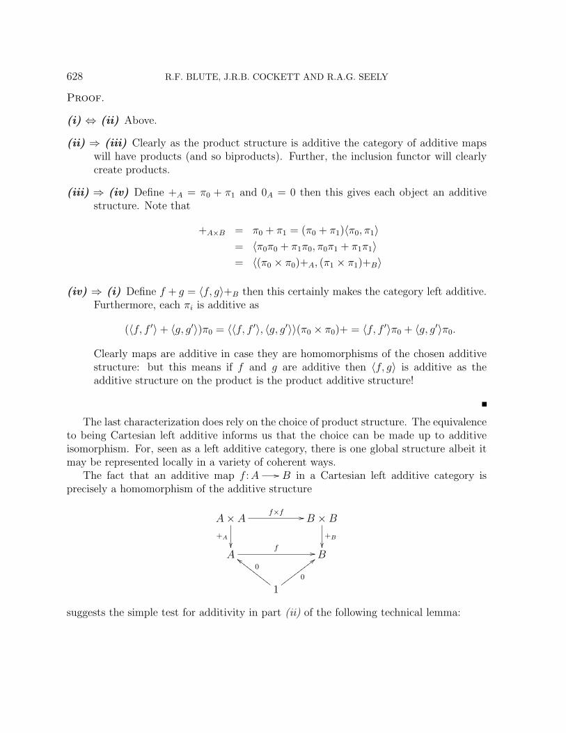
The fact that an additive map f :A // B in a Cartesian left additive category isprecisely a homomorphism of the additive structure

A× A+A

f×f // B ×B+B

A

f // B

1

0

ccFFFFFFFFFF 0

;;wwwwwwwwww

suggests the simple test for additivity in part (ii) of the following technical lemma:


1.2.3. Lemma. In a Cartesian left additive category:

(i) 〈f, g〉+ 〈f ′, g′〉 = 〈f + f ′, g + g′〉 and 0 = 〈0, 0〉;

(ii) f is additive if and only if

(π0 + π1)f = π0f + π1f :A× A // B and 0f = 0: 1 // B;

(iii) g:A×X // B is additive in its second argument if and only if

1×(π0+π1)g = (1×π0)g+(1×π1)g:A×X×X //B and (1×0)g = 0:A×1 //B.

Being additive in the second argument means 〈x, y + z〉g = 〈x, y〉g + 〈x, z〉g and〈x, 0〉g = 0; being additive in an argument is a property which will become more centralshortly.

Proof.

(i) We have the following calculation:

〈f, g〉+ 〈f ′, g′〉 = (〈f, g〉+ 〈f ′, g′〉)〈π0, π1〉= 〈(〈f, g〉+ 〈f ′, g′〉)π0, (〈f, g〉+ 〈f ′, g′〉)π1〉= 〈〈f, g〉π0 + 〈f ′, g′〉π0, 〈f, g〉π1 + 〈f ′, g′〉π1〉= 〈f + f ′, g + g′〉

and a similar calculation for the zero.

(ii) If f is additive this equality holds. Conversely

(h+ k)f = 〈h, k〉(π0 + π1)f = 〈h, k〉(π0f + π1f) = hf + kf.

(iii) Similar.

One reason for demanding that the product structure be additive is the following(which uses the fact that products in additive categories are necessarily biproducts):

1.2.4. Corollary. For any Cartesian left additive category X the subcategory of theadditive maps I: X+

// X has biproducts.

Again we may consider the example CMon: it is clear that letting the product be theusual product of commutative monoids will ensure that we obtain a Cartesian left additivecategory. Note that an arbitrary monoid which has base set the product of the base setsof M1 and M2 will not work as the left additive product as π0 + π1 will no longer give themonoid operation.


1.3. Cartesian left additive functors.

1.3.1. Definition. A functor between Cartesian left additive categories is Cartesianleft additive in case

• F (f + g) = F (f) + F (g) and F (0) = 0;

• F preserves products (i.e F (A) oo F (π0)F (A×B)

F (π1) // F (B) is a product).

Clearly the identity functor is left additive and we may compose Cartesian left addi-tive functors, thus, this, together with natural transformations (whose components areadditive) gives the data for a 2-category. Notice that Cartesian left additive functors pre-

serve the additive structure maps A×A + //A oo 0 1 so, crucially for the 2-dimensionalstructure, we have:

1.3.2. Lemma. A left additive functor is a Cartesian left additive functor if and only ifit preserves additive maps.

Proof. A map is additive if and only if it is a homomorphism of the given additivestructure: this property is preserved by Cartesian left additive functors. The conversefollows as biproducts are equationally defined using the additive maps.

Suppose S = (S, δ, ε) is any comonad (where S need not be Cartesian left additive) on

a Cartesian left additive category, X. Then clearly the coKleisli maps S(X)f //Y inherit

an addition from X and with this XS becomes left additive. (In the following calculation,we shall distinguish maps in the coKleisli category by setting them in boldface; maps inX will be in ordinary type.)

f(g1 + g2) = δS(f)(g1 + g2) = δS(f)g1 + δS(f)g2 = fg1 + fg2

As XS is a coKleisli category it has products inherited from X with

X oo π0 X × Y π1 // Y = X oo επ0 S(X × Y )επ1 // Y.

Note that these projections are additive in XS as

(f + g)π0 = δS(f + g)επ0 = (f + g)π0 = (fπ0) + (gπ0) = (fπ0) + (gπ0)

Consider the pairing map:

Z〈f,g〉 // X × Y = S(Z)

〈f,g〉 // X × Y

and suppose f and g are additive in XS then

(x+ y)〈f,g〉 = δS(x+ y)〈f, g〉 = 〈δS(x+ y)f, δS(x+ y)g〉= 〈(x+ y)f, (x+ y)g〉 = 〈xf + yf, xg + yg〉= 〈xf, xg〉+ 〈yf, yg〉 = x〈f, g〉+ y〈f, g〉

We therefore have:


1.3.3. Proposition. If S = (S, δ, ε) is any comonad on a (Cartesian) left additivecategory X then XS is (Cartesian) left additive. Furthermore the canonical right adjointGS: X // XS is a Cartesian left additive functor.

Proof. The hard work was done above! It remains to check that GS is additive as itclearly preserves products; for this we need

GS(f + g) = ε(f + g) = εf + εg = GS(f) +GS(g) and GS(0) = ε0 = 0.

As an application of Proposition 1.3.3, we note that since a Cartesian left additivecategory X has products, for each object A ∈ X the functor × A is a comonad (usingthe fact that A is canonically a comonoid); the coKleisli category is sometimes known asthe “simple slice category at A”; we shall denote it X[A]:

1.3.4. Definition. X[A] (called “the simple slice category at A”) has as objects theobjects of X, and as morphisms f :X // Y morphisms f :X×A //Y of X. Identities are

given by projections, and composition is the coKleisli composition: Xf // Y

g // Z =

X × A ∆×1 // X × A× A 1×f // Y × A g // Z.

1.3.5. Corollary. Each simple slice X[A] of a Cartesian left additive category X is aCartesian left additive category.

Notice that the additive functions in X[A] are exactly the maps f :X ×A // Y whichare additive in their first argument in the sense that 〈x + y, z〉f = 〈x, z〉f + 〈y, z〉f and〈0, z〉f = 0.

1.4. Cartesian closed left additive categories. A left additive category is aCartesian closed left additive category in case it is a Cartesian left additive categorywhich is Cartesian closed, so A × is a left adjoint with right adjoint A ⇒ , such thatthe passage:

A×X f // YX

curry(f)// A⇒ Y

preserves the additive structure. That is curry(f+g) = curry(f)+curry(g) and curry(0) =0.

1.4.1. Lemma. A Cartesian left additive category X is a Cartesian closed left additivecategory if and only if X is Cartesian closed and

A⇒ B × A⇒ B

k×

+A⇒B=π0+π1 // A⇒ B

A⇒ (B ×B)A⇒+B=A⇒(π0+π1)

44jjjjjjjjjjjjjjjj

10 //

k1

A⇒ B

A⇒ 1A⇒0

55lllllllllllll

commute.


Proof. “Only if” is obvious by considering adjoints. For the converse, we note that whenthe stated condition holds we have:

curry(f + g) = curry(〈f, g〉)(A⇒ +B)

= 〈curry(f), curry(g)〉k×(A⇒ +B)

= 〈curry(f), curry(g)〉+A⇒B = curry(f) + curry(g)

so that addition is preserved by currying: the preservation of zero is similar. Thus, thecategory is Cartesian closed left additive.

When a category is Cartesian closed then (A⇒ , η, µ) is a monad for each object Awhere

A×X π1 // XX

curry(π1)// A⇒ Y

η

A× (A⇒ (A⇒ X))∆×1 // A× A× (A⇒ (A⇒ X))

1×eval // A× (A⇒ X) eval // X

A⇒ (A⇒ X)curry((∆×1)(1×eval)eval)

// A⇒ Xµ

The Kleisli category for this monad is clearly isomorphic to X[A] and the coherencerequirement for closedness ensures that the two additive structures inherited from X,regarding it as a Kleisli and coKleisli category respectively, coincide.

In particular note that in a Cartesian closed left additive category A × X f // Y is

additive in its second argument if and only if Xcurry(f) //A⇒ Y is additive. Once again

we may consider CMon: this is a Cartesian closed left additive category provided oneendows the hom-sets with the pointwise additive structure f + g = λx.f(x) + g(x).

1.5. Additive bundle fibrations. Of course, there is a well-known fibration associ-ated with the simple slice categories; we are interested in the subfibration whose fibres arejust the additive parts of the simple fibres. We think of this fibration as the fibration of“additive bundles” over X, and so denote it by p: ABun(X) //X. The objects of ABun(X)are pairs (X,A), its morphisms (X,A) //(Y,B) are pairs (F, f) of morphisms of X, whereF :X × A // Y is additive in its first argument, and f :A // B. Composition is definedby (F, f)(G, g) = (〈F, π1f〉G, fg), and the identities are (π0, 1A). We shall check (below)that if F,G are additive in the first variable, so is 〈F, π1f〉G.

ABun(X) has additive structure, defined coordinate-wise: (F, f)+(G, g) = (F+G, f+g), 0 = (0, 0). It also has products: 1 = (1, 1) and

(X,A) oo (π0π0,π0)(X × Y,A×B)

(π0π1,π1) // (Y,B)

In fact:

1.5.1. Proposition. If X is Cartesian left additive, then ABun(X) is as well.


Proof. There are a number of things to check — here are those that are not perfectlyobvious.

Composition preserves additivity in the first component:

〈x+ y, z〉〈F, π1f〉G = 〈〈x+ y, z〉F, zf〉G= 〈〈x, z〉F + 〈y, z〉F, zf〉G= 〈〈x, z〉F, zf〉G+ 〈〈y, z〉F, zf〉G= 〈x, z〉〈F, π1f〉G+ 〈y, z〉〈F, π1f〉G

Addition is well-defined (i.e. F +G is additive in the first variable):

〈x+ y, z〉(F +G) = 〈x+ y, z〉F + 〈x+ y, z〉G= 〈x, z〉F + 〈x, z〉G+ 〈y, z〉F + 〈y, z〉G= 〈x, z〉(F +G) + 〈y, z〉(F +G)

(F +G, f + g) is left additive:

(H, h)(F +G, f + g) = (〈H, π1h〉(F +G), h(f + g))

= (〈H, π1h〉F + 〈H, π1h〉G, hf + hg)

= (〈H, π1h〉F, hf) + (〈H, π1h〉G, hg)

= (H, h)(F, f) + (H, h)(G, g)

Products: Given

(X,A) oo (F,f)(Z,C)

(G,g) // (Y,B)

the induced map to the product is simply (Z,C)(〈F,G〉,〈f,g〉) // (X × Y,A×B). The point

then is that this commutes as required, is unique, and finally that the projections areadditive, and that pairing preserves additivity. One useful observation is that (F, f) isadditive (in ABun(X)) if and only if both F, f are additive (in X).

(〈F,G〉, 〈f, g〉)(π0π0, π0) = (〈〈F,G〉, π1〈f, g〉〉π0π0, 〈f, g〉π0)

= (F, f)

and similarly for the other composite. Note that this also shows uniqueness, since thetyping of the “fill map” (Z,C) // (X ×Y,A×B) forces it to be (〈F,G〉, 〈f, g〉), providedthat commutes as required.

The projectives are additive:

((F, f) + (G, g))(π0π0, π0) = (F +G, f + g)(π0π0, π0)

= (〈F +G, π1(f + g)〉π0π0, (f + g)π0)

= ((F +G)π0, (f + g)π0)

= (Fπ0 +Gπ0, fπ0 + gπ0)

= (Fπ0, fπ0) + (Gπ0, gπ0)

= (F, f)(π0π0, π0) + (G, g)(π0π0, π0)


and similarly for π1.

Pairing preserves additivity: suppose (F, f), (G, g) are additive (so all F, f,G, g are). Then

((H, h) + (K, k))(〈F,G〉, 〈f, g〉)= (H +K,h+ k)(〈F,G〉, 〈f, g〉)= (〈H +K, π1(h+ k)〉〈F,G〉, (h+ k)〈f, g〉)= (〈H +K, π1(h+ k)〉F, 〈H +K, π1(h+ k)〉G〉, 〈(h+ k)f, (h+ k)g〉)= (〈(H, π1h)F + (K, π1k)F, (H, π1h)G+ (K, π1k)G〉, 〈hf + kf, hg + kg〉)= (〈(H, π1h)F, (H, π1h)G〉, 〈hf, hg〉) + (〈(K, π1k)F, (K, π1k)G〉, 〈kf, kg〉)= (H, h)(〈F,G〉, 〈f, g〉) + (K, k)(〈F,G〉, 〈f, g〉)

Next we consider the “projection” functor p: ABun(X) // X which sends (X,A) 7→ A,(F, f) 7→ f ; this is well-known to be a fibration, but there is more structure in our context:it is clear that p preserves ×,+, and so is a Cartesian left additive functor. Hence:

1.5.2. Proposition. If X is Cartesian left additive, then p: ABun(X) // X is a Carte-sian left additive functor which is also a fibration, whose fibres are additive categories.

We can axiomatize the essence of this structure:

1.5.3. Definition. p: Y //X is a additive bundle fibration if it is a fibration satisfyingthese properties.

1. X is left additive;

2. each fibre p−1A is additive, for every object A of X;

3. f ∗: p−1B // p−1A is additive, for every morphism Af // B of X;

4. there is an object function ( , ): Obj(X × Y) // Obj(Y) so that for any morphism

Af // B of X, the Cartesian lifting of f to any object X over B is of the form

f : (X,A) // X, or in other words, f ∗X = (X,A), and does not depend on f butmerely on X and the domain of f .

Note that in this definition we have not assumed that Y is left additive (even if fromABun(X) we expect it to be), nor have we supposed that X and Y are Cartesian. Thefirst non-supposition turns out to be unnecessary, as the next Proposition shows. As forthe second, we see that if X and the fibres are Cartesian, then so must Y be also. (Thisis familiar territory from fibrations, of course.)

1.5.4. Proposition. If p: Y // X is an additive bundle fibration, then

1. Y is left additive with respect to the additive bundle addition, and

2. if each p−1A is Cartesian additive and if X is Cartesian left additive, then Y isCartesian left additive as well.


Proof. We shall use the following notation: if f :Y // X is a morphism of Y over the

morphism Apf //B in X, then its factorization into a fibre map followed by a Cartesian

map over pf will be written Yf ′ // (X,A)

pf // X. Then we may define the additivestructure as follows: 0 = 0; 0, where we use 0 to denote the 0-map in the fibre over A, aswell as the 0-map in Y and X, and f+g = (f ′+g′); (pf + pg). This is clearly commutative;furthermore 0 is a unit for +, and + is associative:

f + 0 = (f ′ + 0)(pf + 0)

= f ′; pf = f

(f + g) + h = (f ′ + g′ + h′)(pf + pg + ph) = f + (g + h)

We need to show Y is left additive.

f(h+ k) = f ; (h′ + k′); (ph+ pk)

= f ′; pf ; (h′ + k′); (ph+ pk)

= f ′; (f ∗h′ + f ∗k′); pf ; (ph+ pk)

= (f ′f ∗h′ + f ′f ∗k′); (p(fh) + p(fk))

= ((fh)′ + (fk)′); (p(fh) + p(fk)) (by uniqueness of factorization)

= fh+ fk

f0 = (f ′pf)(00)

= f ′f ∗0(pf)(p0)

= f ′0(p0) = 00

Now, we suppose that the base category and the fibres are Cartesian; note that each f ∗

is additive, so preserves products. Products in Y are defined in the standard manner,pulling back to a common fibre and forming the product there. We must show that theprojections are additive, and that the pair of additive maps is additive. We shall find thefollowing lemma useful here.

1.5.5. Lemma. Any map f in Y is additive if and only if f ′ and pf are additive, in thefollowing sense: for suitably typed maps h, k, the following equations hold: ((h + k)f)′ =(hf)′ + (kf)′ and p((h+ k)f) = p(hf + kf).

Proof. (of the lemma) The fibre-map factor of (h + k)f is (h′ + k′)(ph + pk)∗f ′ =((h+ k)f)′, and the Cartesian factor is (ph+ pk)pf = (ph+ pk)pf . The fibre-map factorof hf+kf is h′(ph)∗f ′+k′(pk)∗f ′ = (hf)′+(kf)′, and the Cartesian factor is p(hf) + p(kf).The lemma is obvious from these factorizations.


So obviously the projections are additive; additionally 〈f, g〉 is additive if f, g are.

(〈hf, hg〉+ 〈kf, kg〉)′ = 〈hf, hg〉′ + 〈kf, kg〉′

= 〈(hf)′, (hg)′〉+ 〈(kf)′, (kg)′〉= 〈(hf)′ + (kf)′, (hg)′ + (kg)′〉= 〈((h+ k)f)′, ((h+ k)g)′〉

p(〈hf, hg〉+ 〈kf, kg〉) = 〈p(hf), p(hg)〉+ 〈p(kf), p(kg)〉= 〈p(hf) + p(kf), p(hg) + p(kg)〉= 〈p(hf + kf), p(hg + kg)〉= 〈p((h+ k)f), p((h+ k)g)〉

We have essentially already shown that ABun(X) //X is an additive bundle fibration;Proposition 1.5.2 may be restated as follows:

1.5.6. Proposition. If X is left additive, then p: ABun(X) // X is an additive bun-dle fibration. Furthermore, if X is Cartesian left additive, then p: ABun(X) // X is aCartesian left additive functor.

2. Cartesian differential categories

Having developed the structure of left additive categories we are now ready to introducethe notion of a Cartesian differential category. Fundamental to these categories is the(appropriate) notion of a differential operator.

Consider the category of finite dimensional vector spaces over (for example) the reals,with homomorphisms which are infinitely differentiable maps. This is left additive, it hasproducts, and furthermore has a natural “differential operator” given by the Jacobian.For example, consider the map f(x1, x2) = x2

1 +x22: IR2 //IR. Its Jacobian is

[2x1

2x2

]. Note

that the Jacobian produces from the point (x1, x2) a linear map from IR2 // IR, and so(“uncurrying”) we get D×(f): IR2 × IR2 // IR. It is this property that we shall abstractwith the notion of a “Cartesian differential operator”.

2.1. The basic definitions.

2.1.1. Definition. An operator D× on the maps of a Cartesian left additive category

Xf // Y

X ×XD×[f ]

// Y

is a Cartesian differential operator in case it satisfies the following:

[CD.1] D×[f + g] = D×[f ] +D×[g] and D×[0] = 0


[CD.2] 〈h+ k, v〉D×[f ] = 〈h, v〉D×[f ] + 〈k, v〉D×[f ] and 〈0, v〉D×[f ] = 0

[CD.3] D×[1] = π0, D×[π0] = π0π0 and D×[π1] = π0π1

[CD.4] D×[〈f, g〉] = 〈D×[f ], D×[g]〉

[CD.5] D×[fg] = 〈D×[f ], π1f〉D×[g]

[CD.6] 〈〈g, 0〉, 〈h, k〉〉D×[D×[f ]] = 〈g, k〉D×[f ]

[CD.7] 〈〈0, h〉, 〈g, k〉〉D×[D×[f ]] = 〈〈0, g〉, 〈h, k〉〉D×[D×[f ]]

Note that the nullary case of [CD.4], D×[〈〉] = 〈〉, automatically holds, since 1 is terminal.[CD.6] may equivalently be stated as

(〈1, 0〉 × 1)D×[D×[f ]] = (1× π1)D×[f ]

Somewhat less obviously (but rather crucially for what follows):

2.1.2. Lemma. [CD.7] is equivalent to [CD.7′]:

〈〈〈0, 0〉, 〈h, 0〉〉, 〈〈0, g〉, 〈k1, k2〉〉〉D×[D×[f ]] = 〈〈〈0, 0〉, 〈0, g〉〉, 〈〈h, 0〉, 〈k1, k2〉〉〉D×[D×[f ]]

Proof. It is clear that this is implied by [CD.7]; to establish the converse, consider thatby [CD.7′]

〈〈0, 〈h, 0〉〉, 〈〈0, g〉, 〈0, k〉〉〉D[D[(π0 + π1)f ]] = 〈〈0, 〈0, g〉〉, 〈〈h, 0〉, 〈0, k〉〉〉D[D[(π0 + π1)f ]]

But

D[D[(π0 + π1)f ]] = ((π0 + π1)× (π0 + π1))× ((π0 + π1)× (π0 + π1))D[D[f ]]

since (anticipating Definition 2.2.1 and Lemma 2.2.2) (π0 +π1) is linear, and so we obtain[CD.7].

2.1.3. Remark. Some comments on these axioms might help the reader with theirmeanings. [CD.1] says D is linear; [CD.2] that it is additive in its first coordinate.[CD.3,4] assert that D behaves coherently with the product structure, and [CD.5] isthe chain rule. We shall see from the proof of Lemma 2.2.2 (v) that [CD.6] is essentiallyrequiring that D×[f ] be linear (in the sense of Definition 2.2.1) in its first variable (moreprecisely, that 〈1, 0〉D×[f ] is linear).

[CD.7] will be clearer when we restate it with a term logic: at that time it will be

clear that [CD.7] is just “independence of order of partial differentiation”: ∂2f∂x∂y

= ∂2f∂y∂x

.


2.1.4. Definition. A Cartesian left additive category which has a Cartesian differentialoperator is a Cartesian differential category.

The category of finite dimensional vector spaces with smooth maps is an example. 2

Here we can define a smooth differential operator via the Jacobi matrix:

Ds[(f1, .., fn)](x, y) = [(∂xifj)(y)]m,ni=1,j=1 x

where x = (x1, ..., xm) and y = (y1, .., ym).

2.2. The subcategory of linear maps. In a Cartesian differential category, notonly is there a subcategory of additive maps but there is also a subcategory of mapswhose differential is constant, that is maps which are “linear”:

2.2.1. Definition. A map in a Cartesian differential category is said to be linear incase D×[f ] = π0f .

The following lemma establishes the basic properties of the linear maps in a Cartesiandifferential category.

2.2.2. Lemma. In any Cartesian differential category

(i) Every linear map is additive;

(ii) 0 is a linear map, and if f and g are linear then f + g is linear;

(iii) Linear maps compose, and include the identity maps;

(iv) Projections are linear and pairings of linear maps are linear;

(v) 〈1, 0〉D×[f ] is linear;

(vi) If a and b are linear and if the lefthand square commutes then the righthand squarealso commutes.

A

a

f // B

b

A′f ′

// B′

=⇒A× Aa×a

D×[f ] // B

b

A′ × A′D×[f ′]

// B′

(vii) If g is a retraction and linear and gh is linear then h is linear;

(viii) If f is an isomorphism and linear then f−1 is linear.

2Indeed this is true of any differential theory over a rig [BCS 06], and so this gives a large class ofexamples.


Proof.

(i) Consider (f + g)h where D×[h] = π0h then

(f + g)h = 〈f + g, f〉D×[h] = 〈f, f〉D×[h] + 〈g, f〉D×[h] = fh+ gh.

(ii) D×[0] = 0 = π00 so the zero map is linear. When f and g are linear then

D×[f + g] = D×[f ] +D×[g] = π0f + π0g = π0(f + g).

(iii) Identity maps by definition are linear. Suppose f and g are linear, thenD×[fg] = 〈D×[f ], π1f〉D×[g] = 〈π0f, π1f〉π0g = π0fg.

(iv) Projections are linear by definition. The pairing of two linear maps is linear asD×[〈f, g〉] = 〈D×[f ], D×[g]〉 = 〈π0f, π0g〉 = π0〈f, g〉.

(v) We have the following calculation:

D×[〈1, 0〉D×[f ]] = 〈D×[〈1, 0〉], π1〈1, 0〉〉D×[D×[f ]]

= 〈π0〈1, 0〉, π1〈1, 0〉〉D×[D×[f ]]

= (1× 〈1, 0〉)(〈1, 0〉 × 1)D×[D×[f ]]

= (1× 〈1, 0〉)(1× π1)D×[f ]

= π0〈1, 0〉D×[f ].

(vi) If af ′ = fb then D×[af ′] = D×[fb] but now

D×[af ′] = 〈D×[a], π1a〉D×[f ′] = 〈π0a, π1a〉D×[f ′] = (a× a)D×[f ′]

D×[fb] = 〈D×[f ], π1f〉D×[b] = 〈D×[f ], π1f〉π0b = D×[f ]b

showing that the above inference holds.

(vii) Let g′g = 1 we need to determine the value of D×[h] for this we have:

D×[h] = (g′ × g′)(g × g)D×[h] = (g′ × g′)〈π0g, π1g〉D×[h]

= (g′ × g′)〈D×[g], π1g〉D×[h] = (g′ × g′)D[gh]

= (g′ × g′)π0gh = π0g′gh = π0h.

(viii) This follows easily from the property above.


From Lemma 2.2.2 we may conclude:

2.2.3. Corollary. The linear maps of a Cartesian differential category form an addi-tive category Xlin which has biproducts. The inclusion I: Xlin

// X reflects isomorphismsand creates products.

2.3. An additive interlude!. In a Cartesian differential category the additive mapsplay second fiddle to the linear maps. Nonetheless they are an important class whichhave many of the properties of the linear maps. Below we develop some of the specialproperties of additive maps before turning our attention to the linear maps.

As a consequence (Corollary 2.3.3), we shall also show that axiom [CD.6] is indepen-dent of the other axioms. (A proof that axiom [CD.7] is independent of the other axiomsmay be constructed from a modification of the construction of the free Cartesian differ-ential category; that will appear in a sequel which develops the technical tools needed forthat construction.)

2.3.1. Proposition. In a Cartesian differential category if f is additive then D×[f ] isadditive and, furthermore, D×[f ] = π0D0[f ] where D0[f ] = 〈1, 0〉D×[f ].

Proof. Suppose f is additive so that π0f + π1f = (π0 + π1)f then

π0D×[f ] + π1D×[f ] = ex(〈π0π0, π1π0〉D×[f ] + 〈π0π1, π1π1〉D×[f ])

= ex(〈D×[π0], π1π0〉D×[f ] + 〈D×[π1], π1π1〉D×[f ])

= ex(D×[π0f ] +D×[π1f ]) = exD×[π0f + π1f ] = exD×[(π0 + π1)f ]

= ex〈D×[π0 + π1], π1(π0 + π1)〉D×[f ]

= ex〈π0(π0 + π1), π1(π0 + π1)〉D×[f ]

= (π0 + π1)D×[f ]

where ex = 〈〈π0π0, π1π0〉, 〈π0π1, π1π1〉〉 is the “exchange” map.Now, when f is additive, we can use the fact D×[f ] is additive to conclude:

D×[f ] = 〈π0, π1〉D×[f ]

= 〈0 + π0, π1 + 0〉D×[f ]

= (〈0, π1〉+ 〈π0, 0〉)D×[f ]

= 〈0, π1〉D×[f ] + 〈π0, 0〉D×[f ]

= 〈π0, 0〉D×[f ]

= π0〈1, 0〉D×[f ]

so that D×[f ] = π0〈1, 0〉D×[f ] = π0D0[f ].

In the extremal situation when every map is additive we may now conclude that thedifferential D×[f ] = π0D0[f ] is given by D0 which is an additive endofunctor stationaryon objects and linear maps and delivers linear maps and so is idempotent.


2.3.2. Corollary. In a Cartesian differential category X in which all maps are additiveD0: X // X is an additive endofunctor which is stationary on all objects and linear mapsand has image the linear maps. Conversely, an endofunctor D0 which is stationary on ob-jects and idempotent endows such a category with a differential operator D×[f ] = π0D0[f ].

Proof. If f is linear then D0[f ] = 〈1, 0〉D×[f ] = 〈1, 0〉π0f = f . As

D0[f+g] = 〈1, 0〉D×[f+g] = 〈1, 0〉(D×[f ]+D×[g]) = 〈1, 0〉D×[f ]+〈1, 0〉D×[g] = D0[f ]+D0[g]

so that D0 preserves addition, it also clearly preserves the zero. D0 preserves compositionas:

D0[fg] = 〈1, 0〉D×[fg] = 〈1, 0〉〈D×[f ], π1f〉D×[g] = 〈〈1, 0〉D×[f ], 0〉D×[g] = D0[f ]D0[g].

For the converse suppose D0: X // X is a functor which is additive, stationary onobjects, and has is idempotent. It preserves the biproduct structure as all additive functorsdo. Now defineD×[f ] = π0D0(f) then it is easy to check that this is a Cartesian differentialoperator.

These observations yield some unexpected examples of Cartesian differential cate-gories.

First consider the category of matrices over the complex numbers (the objects beingnatural numbers and the maps being matrices) then there is an obvious endofunctor whichtakes the complex conjugate of each matrix entry. This leaves the product structureuntouched. This makes it a (non-trivial) additive endo functor which however is notidempotent. By treating this as the D0 of corollary 2.3.2 we get a structure D×[f ] =π0D0[f ] which satisfies all the equations except [CD.6]. This means:

2.3.3. Corollary. [CD.6] is independent of the rest of the axioms.

To get an example of a structure which also satisfies this axiom it suffices to consider aring with a retraction: for example the polynomial ring over the complex numbers retractonto the complexes by assigning the indeterminate to any number:

rx:=0: C[x] // C.

This extends to an additive idempotent endofunctor on the category of the matrices overC[x] which can serve as the endofunctor D0 in the above. This makes the matrices withentries in C the linear maps and the rest have a differential which collapses back to C.

Clearly, an interesting case is when the linear maps and additive maps coincide. Onemay express this by the requirement that D0 is the identity functor on the additive maps.The example above shows that this, if desired, is an extra requirement.

2.3.4. Corollary. There are Cartesian differential categories where the additive mapsare not all linear.

It seems appropriate to make one further remark about the operatorD0[f ] = 〈1, 0〉D×[f ].One should think of it as giving the differential at 0. Of course, when one fixes the point


at which one takes the differential one obtains an additive map. Therefore, let X0 be thesubcategory of X determined by those maps which preserve the zero (0f = 0). Clearlyany D×[f ] preserves the 0 by [CD.2], thus X0 is itself a Cartesian differential subcategorywhich will usually strictly include all the additive maps.

2.3.5. Corollary. If X is a Cartesian differential category then X0, consisting of themaps which preserve 0 (i.e. satisfying 0f = 0), is a Cartesian differential subcategory.

A further class of maps should be mentioned namely the constant maps, that isthose with differential zero. Classically they are important as the differential of a mapwill not be changed by adding constant maps to it.

2.4. Cartesian differential operators and the bundle fibration. Recall(Section 1.5) that if X is Cartesian left additive, then p: ABun(X) // X is an additivebundle fibration, and p: ABun(X) // X is a Cartesian left additive functor.

Suppose p: ABun(X) // X has some further structure: suppose p has a left additivesection D: X // ABun(X). Some interesting consequences follow from this supposition,consequences which one may take as motivation for the axioms of a Cartesian differentialoperator.

First, some notation: let’s write D(A) = (d0(A), A) and D(f) = (D×[f ], f), for A anobject of X, and f :A // B a map of X. (The assumption that D is a section forces thesecond component to be as given.) Note then that D×[f ]: d0(A)×A // d0(B) is additivein its first component. Also, that D is a functor forces the following equation:

〈D×[f ], π1f〉D×[g] = D×[fg]

because the lefthand side is the first component of D(f)D(g) and the righthand side is thefirst component of D(fg). (In each case the second component is just fg.) Our view willbe that ABun(X) captures differential structure of X, and that composition in ABun(X)should then be governed by the chain rule — this is exactly what the equation aboveexpresses.

In addition, that D preserves identities means that 1 = (π0, 1) = (D×[1], 1), and so

D×[1] = π0

Also D(π0) = (π0π0, π0), soD×[π0] = π0π0

SimilarlyD×[π1] = π0π1

D preserves +: D(f + g) = D(f) +D(g), and so

D×[f + g] = D×[f ] +D×[g]

So what we see here is that part of the definition of Cartesian differential operator(Definition 2.1.1), specifically [CD.1-5], follows immediately from the existence of a leftadditive section D to p.


But we can in fact push this analysis of the additive bundle fibration further: wecan define the notion of “linear map” in this context. We say a map f of X is linear ifD×[f ] = π0g for some g. Then we note that the basic properties of linear maps hold inthis generality, with more or less the same proofs.

• g is uniquely determined by f (since π0: d0A × A // d0A is epi, having a section〈1, 0〉). We shall denote the map g by d0(f).

• d0 so defined is an endo-functor on X, and linear maps form an additive subcategoryof X.

– D×[1] = π0, so identities are linear;

– if D×[f ] = π0d0f and D×[g] = π0d0g, then D×[fg] = 〈D×[f ], π1f〉D×[g] =〈π0f0f, π1f〉π0d0g = π0d0fd0g, so linear maps are closed under composition;

– if f, g are linear, then D×[f + g] = D×[f ] + D×[g] = π0d0f + π0d + 0g =π0(d0f + d0g), so f + g is linear as well.

• If f is additive, then so is d0f :

(x+ y)d0f = 〈x+ y, 0〉π0d0f

= 〈x+ y, 0〉D×[f ]

= 〈x, 0〉D×[f ] + 〈y, 0〉D×[f ]

= 〈x, 0〉π0d0f + 〈y, 0〉π0d0f

= xd0f + yd0f

• Projections are linear; pairs of linear maps are linear.

The special case which concerns us is when the functor d0 is the identity (we suggestcalling D stationary in this case). When that is so, then we have the rest of the basicproperties:

• If a and b are linear and if the lefthand square commutes then the righthand squarealso commutes.

A

a

f // B

b

A′f ′

// B′

=⇒A× Aa×a

D×[f ] // B

b

A′ × A′D×[f ′]

// B′

• If g is a retraction and linear and gh is linear then h is linear.

• Hence, if f is an isomorphism and linear then f−1 is linear.


A proper analysis in this fashion of [CD.6,7] involves higher order differential struc-ture: just as the chain rule essentially characterizes composition in additive bundle fibra-tions, the higher order chain rules induce a family of such fibrations, the Faa di Brunofibrations, corresponding to higher order differential structure — a well-behaved compo-sition in the second order Faa di Bruno fibration will motivate [CD.6,7] in a similarmanner (the details are somewhat technical, and will be presented in a sequel).

3. The coKleisli category of a differential category

First, we shall recall some definitions from [BCS 06], and set our notation.

3.1. Differential categories. A coalgebra modality on an additive (i.e. com-mutative monoid enriched) symmetric monoidal category X is a comonad (S, δ, ε) so thateach object S(X) is a coalgebra or comonoid (S(X),∆, e) and δ is a comonoid morphism.

∆:S(X) // S(X)⊗ S(X) e:S(X) //>

S(X)

∆ NNNNNNNNNNN

NNNNNNNNNNN

ppppppppppp

ppppppppppp

S(X) S(X)⊗ S(X)1⊗e

ooe⊗1

// S(X)

S(X) ∆ //

∆

S(X)⊗ S(X)

∆⊗1

S(X)⊗ S(X)1⊗∆

// S(X)⊗ S(X)⊗ S(X)

S(X) δ //

e""EE

EEEE

EES(S(X))

ezzvvv

vvvvvv

v

>

S(X) δ //

∆

S(S(X))

∆

S(X)⊗ S(X)δ⊗δ

// S(S(X))⊗ S(S(X))

(We wrote ! instead of S in [BCS 06]; S will fit better with the rest of this paper.)Note that we do not require X to have biproducts. On such a category, a differentialcombinator D⊗: X(S(A), B) // X(A⊗ S(A), B) is a natural combinator satisfying fouraxioms (we suppress structural isomorphisms):

[D.1] (Constant maps) D⊗[eA] = 0

[D.2] (Product rule) D⊗[∆(f ⊗ g)] = (1⊗∆)(D⊗[f ]⊗ g) + (1⊗∆)(c⊗ 1)(f ⊗D⊗[g]),where f :S(A) // B, g:S(A) // C, and c is the commutativity isomorphism

[D.3] (Linearity) D⊗[εAf ] = (1⊗ eA)f , where f :A // B

[D.4] (Chain rule) D⊗[δ S(f) g] = (1⊗∆)(D⊗[f ] ⊗ δS(f))D ⊗ [g] where f :S(A) // Band g:S(B) // C.

A differential category is an additive symmetric monoidal category with a coalgebramodality and a differential combinator. The structure of the differential combinator mayalso be described in slightly simpler terms using a “deriving transformation” d⊗: = D⊗[1].


(The four axioms have a slightly simpler formulation in terms of d⊗.) In [BCS 06] we usedthe notation D and d; in this paper we also have similar “Cartesian” operations D×, d×for Cartesian differential categories, so we shall use the subscripted D⊗, d⊗ to distinguishthe differential combinator and deriving transformation of a differential category fromtheir counterparts in a Cartesian differential category.

In [BCS 06], we also define several “richer” variants of differential categories: forexample, if X has biproducts, we define a differential storage category as an additivestorage category with a deriving transformation such that the “∇-rule” (d⊗1)∇ = (1⊗∇)dis satisfied, (∇ being the codiagonal, part of the bialgebra structure). Being a storagecategory means that the coalgebra modality is symmetric monoidal, and the comonoidstructure is a morphism for the coalgebras. This is equivalent to the induced tensor onthe coalgebras being a product, and in fact in this setting we obtain the storage (orSeely) isomorphisms which mediate a canonical bialgebra structure on the cofree objectsby transporting the bialgebra structure on the biproduct. The point about differentialstorage categories from our present viewpoint is that the deriving transformation is givenby the bialgebra structure: dX = (ηX ⊗ 1)∇, for a natural map η.

The reader should consult [BCS 06] for the details of this and the other variants.

3.2. The coKleisli category of a differential category. Our principle ex-ample of a Cartesian differential category arises as the coKleisli category of a differentialcategory. In fact, under reasonable conditions, we may represent Cartesian differentialcategories as the coKleisli categories of differential categories; in order to do that, weneed to consider abstract coKleisli categories in general, which will be the main focus ofa sequel to this paper. But for now, let us consider this example of Cartesian differentialcategories. As before, to distinguish maps in the coKleisli category, we shall representthem in boldface.

The key this example is that, given a differential category X with products (and sobiproducts), it is possible to define a differential combinator on the coKleisli category:

given Xf // Y in the coKleisli category (and so S(X)

f // Y in the underlying cate-gory), we construct D×[f ]:X ×X // Y in the coKleisli category as the arrow (in theunderlying category)

D×[f ] =

S(X ×X) ∆ // S(X ×X)⊗ S(X ×X)Sπ0⊗Sπ1 // S(X)⊗ S(X) ε⊗1 // X ⊗ S(X)

D⊗[f ] // Y

We remark that the arrow

s2: = S(X ×X) ∆ // S(X ×X)⊗ S(X ×X)Sπ0⊗Sπ1 // S(X)⊗ S(X)

is the canonical (inverse) storage isomorphism, in a category which has the storage iso-morphism — for example, for a storage modality. However, we are not supposing thisis an isomorphism here. In fact, having s (and its nullary version) amounts to having acoalgebra modality.


3.2.1. Proposition. The coKleisli category of a differential storage category (withbiproducts) is a Cartesian differential category, whose Cartesian differential combinatoris defined as above.

We must prove the axioms [CD.1-7] hold with this defined D×. In fact, we may relaxthe conditions somewhat for [CD.1-6]: only [CD.7] requires something like storage.

3.2.2. Lemma. [CD.1-6] are valid in the coKleisli category of a differential categorywith biproducts.

Proof.

[CD.1] follows from left additivity.

[CD.2] For Z〈h1+h2,v〉 // X ×X, consider

〈h+ k, v〉D×[f ]

= δ;S(〈h+ k, v〉); ∆;S(π0)⊗ S(π1); ε⊗ 1;D⊗[f ]

= δ; ∆; ε⊗ 1; (h+ k)⊗ S(v);D⊗[f ]

= δ; ∆; ε⊗ 1; (h⊗ S(v) + k ⊗ S(v));D⊗[f ]

= (δ; ∆; ε⊗ 1;h⊗ S(v)D⊗[f ]) + (δ; ∆; ε⊗ 1; k ⊗ S(v)D⊗[f ])

= (δ;S(〈h, v〉); ∆;S(π0)⊗ S(π1); ε⊗ 1;D⊗[f ])

+ (δ;S(〈k, v〉); ∆;S(π0)⊗ S(π1); ε⊗ 1;D⊗[f ])

= 〈h, v〉D×[f ] + 〈k, v〉D×[f ]

[CD.3] Notice that D×[1], being in the coKleisli category, is S(X × X) // X, π0 isreally ε; π0:S(X × X) // X × X // X, and so we consider the following (wehave suppressed the use of the unit isomorphism).

D×[1] = ∆;S(π0)⊗ S(π1); ε⊗ 1;D⊗[ε]

= ∆;S(π0)⊗ S(π1); ε⊗ 1; 1⊗ e= ∆;S(π0)⊗ S(π1); 1⊗ e; ε= ∆; 1⊗ e;S(π0); ε

= S(π0); ε = ε; π0

Next, note that π0π0 is really επ0π0, so we need the following (again suppressingthe use of the unit isomorphism).

D×[π0] = ∆;S(π0)⊗ S(π1); ε⊗ 1;D⊗[επ0]

= ∆;S(π0)⊗ S(π1); ε⊗ 1;π0 ⊗ e= ∆;S(π0)⊗ S(π1); (επ0)⊗ e= ∆; (επ0π0)⊗ e = επ0π0

and similarly for π1.


[CD.4] It suffices to show that D×[〈f, g〉]π0 = D×[f ] and D×[〈f, g〉]π1 = D×[g].We notice first that similar equations hold for D⊗, via the chain rule:

D⊗[f ] = D⊗[〈f, g〉π0]

= 1⊗∆;D⊗[〈f, g〉]⊗ δS(〈f, g〉);D⊗[επ0]

= 1⊗∆;D⊗[〈f, g〉]⊗ δS(〈f, g〉); π0 ⊗ e= 1⊗∆; (D⊗[〈f, g〉]π0)⊗ e= D⊗[〈f, g〉]π0

and similarly for g. Then we see

D×[〈f, g〉]π0 = ∆;S(π0)⊗ S(π1); ε⊗ 1;D⊗[〈f, g〉]; π0

= ∆;S(π0)⊗ S(π1); ε⊗ 1;D⊗[f ]

= D×[f ]

and similarly for g.

[CD.5] Translating from the coKleisli category to the underlying category, we show thefollowing equation. This is moderately complex as a categorical diagram, and soto illustrate the comparative simplicity of the circuits, we shall also prove thiswith circuits in Figures 1 and 2.

δ;S(〈∆, S(π1)f〉);S((Sπ0 ⊗ Sπ1)× 1);S((ε⊗ 1)× 1);S(D⊗[f ]× 1); ∆;Sπ0 ⊗ Sπ1; ε⊗ 1;D⊗[g]

= ∆; δ ⊗ δ;S(〈∆, S(π1)f〉)⊗2;S((Sπ0 ⊗ Sπ1)× 1)⊗

2;S((ε⊗ 1)× 1)⊗

2;S(D⊗[f ]× 1)⊗

2;

Sπ0 ⊗ Sπ1; ε⊗ 1;D⊗[g]

= ∆; δ ⊗ δ;S(〈∆, S(π1)f〉)⊗2;S((Sπ0 ⊗ Sπ1)× 1)⊗

2;S((ε⊗ 1)× 1)⊗

2;S(D⊗[f ]× 1)⊗

2;

ε⊗ 1;π0 ⊗ Sπ1;D⊗[g]

= ∆; 1⊗ δ; (∆⊗ SS(π1)f)⊗2; ((Sπ0 ⊗ Sπ1)× 1)⊗

2; ((ε⊗ 1)× 1)⊗ S((ε⊗ 1)× 1);

(D⊗[f ]× 1)⊗ S(D⊗[f ]× 1);π0 ⊗ Sπ1;D⊗[g]= ∆; 1⊗ δ; ∆⊗ SS(π1)f ; (Sπ0 ⊗ Sπ1)⊗ 1; (ε⊗ 1)⊗ 1;D⊗[f ]⊗ 1;D⊗[g]= ∆; 1⊗∆; 1⊗ 1⊗ δ; 1⊗ 1⊗ SS(π1)f ; (Sπ0 ⊗ Sπ1)⊗ 1; (ε⊗ 1)⊗ 1;D⊗[f ]⊗ 1;D⊗[g]= ∆; 1⊗∆; (Sπ0 ⊗ Sπ1)⊗ Sπ1; (ε⊗ 1)⊗ 1;D⊗[f ]⊗ δS(f);D⊗[g]= ∆;Sπ0 ⊗ Sπ1; 1⊗∆; (ε⊗ 1)⊗ 1;D⊗[f ]⊗ δS(f);D⊗[g]= ∆;Sπ0 ⊗ Sπ1; ε⊗ 1;D⊗[δS(f)g]

As mentioned above, the corresponding circuit manipulations are shown in Fig-ures 1 and 2. We should point out that we use two different types of circuit boxesin these circuits: those with a half-oval marking the principal port are storageboxes (much like Girard’s original boxes for ! [G 87]), and the box without thehalf-oval in the first circuit is a product box (like our linear functor boxes [CS99]).


[CD.6] In XS (1× π1)D×[f ] is the X map

(1× π1)D×[f ]

= S(1× π1); ∆;S(π0)⊗ S(π1); ε⊗ 1;D⊗[f ]

= ∆;S(π0)⊗ S(π1π1); ε⊗ 1;D⊗[f ]

= ∆; (επ0 ⊗ S(π1π1)); d⊗; f

This is displayed as a circuit in Figure 3.

Before we deal with the coKleisli map (〈1, 0〉 × 1)D×[D×[f ]], we simplify themap D⊗[D×[f ]] (needed to “decode” D×[D×[f ]] in the coKleisli category):

D⊗[D×[f ]]

= D⊗[∆; (S(π0)ε)⊗ S(π1);D⊗[f ]]

= d⊗; ∆; (S(π0)ε)⊗ S(π1); d⊗; f

= (1⊗∆); (d⊗ ⊗ 1); επ0 ⊗ S(π1); d⊗; f

+(1⊗∆); (c⊗ 1); (1⊗ d⊗); επ0 ⊗ S(π1); d⊗; f

= (1⊗∆); (1⊗ e⊗ 1); (π0 ⊗ S(π1)); d⊗; f

+(1⊗∆); (c⊗ 1); (1⊗ (π1 ⊗ S(π1)); (επ0 ⊗ d⊗); d⊗; f

= π0 ⊗ S(π1); d⊗; f + (1⊗∆); (c⊗ 1); (1⊗ (π1 ⊗ S(π1)); (επ0 ⊗ d⊗); d⊗; f

In circuits, this is displayed in Figure 4.

Finally, we may complete the proof with the following calculation.

(〈1, 0〉 × 1)D×[D×[f ]]

= S(〈1, 0〉 × 1); ∆;S(π0)⊗ S(π1); ε⊗ 1;D⊗[D×[f ]]

= ∆; επ0〈1, 0〉 ⊗ S(π1); π0 ⊗ S(π1); d⊗; f

+ ∆; επ0〈1, 0〉 ⊗ S(π1); (1⊗∆); (c⊗ 1); (1⊗ (π1 ⊗ S(π1)); (επ0 ⊗ d⊗); d⊗; f

= ∆; επ0 ⊗ S(π1π1); d⊗; f

+ ∆; (ε0⊗∆); (c⊗ 1); (1⊗ S(π1π1)); (ε⊗ d⊗); (π1π0 ⊗ 1); d⊗; f

= ∆; επ0 ⊗ S(π1π1); d⊗; f + 0

= ∆; επ0 ⊗ S(π1π1); d⊗; f

= (1× π1)D×[f ]

as hoped for. This calculation is displayed in Figure 5.


g

f

∆

∆

ε

ε f

π0

π0

π1

π1 π1

ε

ε

ε

ε ε

S(X ×X)

S(X ×X)

S(X ×X)

S(Y × Y )

S(X ×X)

S(Y × Y )

S(X ×X)

X ×X

Y × Y

X ×X

Y × Y

X ×X

S(X)

S(Y )

S(X)

S(Y )

S(X)

S(Y )

S(X)

X

Y

Y

Y

Z

Y × Y

S(Y × Y )

X

Y

X

Y

X

=

Figure 1: [CD.5] in XS, continued in Figure 2


g

f

∆

∆

ε

f

π0 π1 π1

ε

ε

ε ε

=

g

f

∆

∆

f

π0 π1 π1

ε ε ε

=

g

f

∆

∆

f

π0 π1 π1

ε ε ε

=

g

f

∆

∆

f

π0 π1

ε ε

=

g

f

∆

ε

π0 π1

ε ε

Figure 2: [CD.5] in XS, continued from Figure 1


f

∆

ε

π0

S(π1π1)

Figure 3: (1× π)D×[f ] in X

f

∆

S(π0)

εS(π1)

f f

∆ ∆

ε ε

π0 π0

S(π1) S(π1)+=

ff

∆

επ0

π0

S(π1)π1 S(π1)

+=

Figure 4: D⊗[D×[f ]] in X


ff

∆

∆

∆

ε

〈1, 0〉

〈1, 0〉ε

ε

π0

π0

π0

π0

S(π1)

S(π1)

S(π1)

π1 S(π1)

+ =

f

∆

ε

π0

S(π1π1)

f

∆

∆

ε

ε

π1π0

0 S(π1π1)

+ =f

∆

ε

π0

S(π1π1)

Figure 5: (〈1, 0〉 × 1)D×[D×[f ]] in X


= ∇ ∇

∇ ∇

η η

η ηCC

CC

CC

CC

=

Figure 6: 1⊗ d⊗; d⊗ = c⊗ 1; 1⊗ d⊗; d⊗

3.2.3. Lemma. In a differential category satisfying the equation 1⊗ d⊗; d⊗ = c⊗ 1; 1⊗d⊗; d⊗, [CD.7] is valid.

Proof. The necessary equation is illustrated in Figure 6.It will be clear that these proofs are more simply presented using the circuit diagrams;

the diagrams for this lemma may be found in Figures 7 and 8. In the diagrams, N denotesthe Cartesian ∆, and the boxes without half-ovals are Cartesian boxes. Note that we haveexpanded D×[D×[f ]] into a sum, similar to what we did in Figures 4, 5.

The proof of Proposition 3.2.1 then follows from the remark that a differential storagecategory has the required property, since there d⊗ = η ⊗ 1;∇, and ∇ is cocommutativeand coassociative, as shown in Figure 6.

3.2.4. Remark. We should note here the following property of the coKleisli categoryof a differential category with biproducts, viz that ε and S(f) (for any f) are linear:

• D×[ε] = π0ε

• D×[S(f)] = π0S(f)

To see the first, recall that ε = εε and π0ε = δS(επ0)εε = επ0ε, so D×[ε] = s(ε ⊗1)D⊗[εε] = s(ε⊗1)(1⊗e)ε = ∆(Sπ0⊗Sπ1)(ε⊗e)ε = ∆(Sπ0⊗e)εε = Sπ0 εε = επ0ε = π0ε.

To see the second, recall that S(f) = εδS(f), so D×[S(f)] = ∆(Sπ0 ⊗ Sπ1)(ε ⊗1)D⊗[εδS(f)] = ∆(Sπ0 ⊗ Sπ1)(ε⊗ e)δS(f) = επ0δS(f) = δS(επ0)εδS(f) = π0S(f).

These equations are central in arriving at an abstract characterization of coKleislicategories of differential categories, the subject of a sequel to this paper.

4. A term calculus for Cartesian differential categories

It is useful to develop a term logic for Cartesian differential categories not only so that themanipulation of maps is facilitated but also to illustrate the extent to which the intuitionsfrom the ordinary calculus of differentiation are captured. The purpose of this section isto provide an account of this term logic.


f

f

∆

∆

∆

π0

π0

π0

π0

π0ε

ε

ε

εε

π0

π0

π1

π1

π1 +

0 h g k

NN

N

f

∆

∆h

k

g

+0=

f

∆

∆h

kg =

f

∆

∆g

k

h

=

Figure 7: 〈〈0, h〉, 〈g, k〉〉D×[D×[f ]]


f

f

∆

∆

∆

π0

π0

π0

π0

π0ε

ε

ε

εε

π0

π0

π1

π1

π1 +

0 g h k

NN

N

=

Figure 8: 〈〈0, g〉, 〈h, k〉〉D×[D×[f ]]


Given a map f :X // Y ;x 7→ t, we shall denote the map D×[f ]:X ×X // Y by theterm

(u, s) 7→ ∂t

∂x(s) · u

where x is a variable of type X, t is a term (representing f) of type Y , and s, u areterms of type X. ∂

∂xbinds occurrences of x in any operator to which it is applied. So in

particular in ∂t∂x

, all occurrences of x in t are bounded. The intention is that ∂t∂x

(s) shoulddetermine a linear transformation, so that in a higher-order system it would be typed as∂t∂x

(s):X − Y . In a first-order system we have to use the uncurried form, and so insist thatthe argument to which it is applied be specified, thus obtaining the term ∂t

∂x(s)·u:Y of type

Y ; this term is assumed to be linear in u. Of course, we think of this as the x-differentialof f , evaluated at x = s. In an “Euler-style” notation, this might be represented by aterm like D[x 7→ t](s) · u. The usual “Leibniz-style” notation is something like ∂t

∂x x:=s.

Remember our convention is that D×[f ] is linear in its first variable, by [CD.2], whichwe have been denoting u here. We denote the function application in this case by “·”(as in “dot product”); in the standard example (“high-school differentiation”) it is in factmatrix multiplication.

For example, if we take for f the function from X: = IR3 to Y : = IR2 given by

f(x, y, z) = (x2 + xyz, z3 − xy), we have ∂〈x2+xyz,z3−xy〉∂(x,y,z)

(r, s, t), a linear transformation

from IR3 to IR2, given by the matrix:(2r + st rt rs−s −r 3t2

)i.e. by the Jacobian evaluated at (r, s, t). We apply this Jacobian to a vector to obtain apoint in IR2:(

2r + st rt rs−s −r 3t2

)· (u, v, w) = ((2r + st)u+ rtv + rsw,−su− rv + 3t2w)

To summarize: this is what we would write in our term logic as

∂(x2 + xyz, z3 − xy)

∂(x, y, z)(r, s, t) · (u, v, w)

(compare this to the categorical notation, D×[f ]: IR3 × IR3 // IR2 which takes the pair((u, v, w), (r, s, t)) to ((2r + st)u + rtv + rsw,−su − rv + 3t2w)). To help keep in mindwhich variables are which, remember that this is supposed to be linear in (u, v, w) (thefirst variable), not necessarily in the second (r, s, t). Of course, a “variable” may be infact a tuple of variables, since we are in a Cartesian category.

4.1. Definition of the term calculus. Explicit term formation rules for the (Carte-sian) differential term logic are given in table 1. The term logic is built assuming that onehas a set of primitive types, T, and that we have a supply Ω of function symbols each with


Γ, x:T ` x:TProj Γ ` t′:T ′

Γ, x:T ` t′:T ′ Weak

Γ ` t′:T ′Γ, (): 1 ` t′:T ′ Unit

Γ, x:T1, y:T2 ` t′:T ′Γ, (x, y):T1 × T2 ` t′:T ′

Pair

Γ ` t1:T1 Γ ` t2:T2

Γ ` (t1, t2):T1 × T2Tuple

Γ ` (): 1UnitTuple

Γ ` t1:T Γ ` t2:TΓ ` t1 + t2:T

AddΓ ` 0:T

Zero

Γ ` ti:Tii=1,..,n f ∈ Ω(T1, ..., Tn;T )

Γ ` f(t1, ..., tn):TFun

Γ, x:S ` t:T Γ ` s:S Γ ` u:S

Γ ` ∂t∂x

(s) · u:TDiff

Γ ` t1:T Γ, x:T ` t2:T ′

Γ ` t2[t1/x]:T ′Cut

Table 1: Terms for Cartesian differential logic

a type in T∗ × T , we write f ∈ Ω(T1, ..., Tn;T ) to indicate a primitive function symbol oftype ([T1, ..., Tn], T ). Here we assume that a context Γ consists of a bag of pattern typepairs. The patterns are created by pairing variables or the unit pattern. In a variablecontext it is always assumed no variable can occurs more than once (i.e. it is linear).

We shall feel free to use n-fold products: these should be interpreted as being con-structed from the binary product using X1 ×X2 × ...×Xn = (. . . (X1 ×X2)× . . .)×Xn

where the association is to the left.The differential operator ∂t

∂xbinds the variable x in t; we assume the usual rules on

bound and free variables, which in general means it is best not to use the same variableboth freely and bound in the same term, and to change bound variables as necessary tomaintain that distinction.

The addition is assumed to be a commutative, associative operation with unit 0. Eachtype therefore contains a 0 and for the final type we have 0: 1 = (): 1

4.1.1. Substitution. The notion t[t′/x] is an explicit substitution term. These termscan be eliminated by the following rewrites which define substitution in this calculus:

[Subst.1] x[t/x]⇒ t and y[t/x]⇒ y if x, y are distinct variables;


[Subst.2] t[(t1, t2)/(p1, p2)]⇒ (t[t1/p1])[t2/p2] and t[()/()]⇒ t;

[Subst.3] (t1, t2)[t/p]⇒ (t1[t/p], t2[t/p]) and ()[t/p]⇒ ();

[Subst.4] f(t1, ..., tn)[t/p]⇒ f(t1[t/p], .., tn[t/p]);

[Subst.5] t1 + t2[t/p]⇒ t1[p/t] + t2[p/t] and 0[t/p]⇒ 0;

[Subst.6] ( ∂t′

∂p′(s) · u)[t/p]⇒ ∂t′[t/p]

∂p′(s[t/p]) · u[t/p];

4.1.2. Equations of terms. There is an equality defined on the differential termlogic, given by the smallest congruence satisfying the following identities.

[Dt.1]∂(t1 + t2)

∂p(s) · u =

∂t1∂p

(s) · u+∂t2∂p

(s) · u and∂0

∂p(s) · u = 0;

[Dt.2]∂t

∂p(s) · (u1 + u2) =

∂t

∂p(s) · u1 +

∂t

∂p(s) · u2 and

∂t

∂p(s) · 0 = 0;

[Dt.3]∂x

∂x(s) · u = u,

∂t

∂(p, p′)(s, s′) · (u, 0) =

∂t[s′/p′]

∂p(s) · u and

∂t

∂(p, p′)(s, s′) · (0, u′) =

∂t[s/p]

∂p′(s′) · u′;

[Dt.4]∂(t1, t2)

∂p(s) · u =

(∂t1∂p

(s) · u, ∂t1∂p

(s) · u)

;

[Dt.5]∂t[t′/p′]

∂p(s) ·u =

∂t

∂p′(t′[s/p]) ·

(∂t′

∂p(s) · u

)(This is the chain rule; we require that

no variable of p occur in t);

[Dt.6]∂ ∂t∂p

(s) · p′

∂p′(r) · u =

∂t

∂p(s) · u.

[Dt.7]∂ ∂t∂p1

(s1) · u1

∂p2

(s2) · u2 =∂ ∂t∂p2

(s2) · u2

∂p1

(s1) · u1

In all these identities we make the usual assumption that they are valid relative to thevariable context consisting of those variables mentioned in the identity.

4.2. Basic properties of the term logic. The following lemma provides somebasic equalities:


4.2.1. Lemma.

(i) ∂t∂()

() · () = 0;

(ii) ∂t∂p

(s) · u = 0 when no variable in p occurs in t;

(iii) ∂t∂(p,p′)

(s, s′) · (u, u′) = ∂t∂p

(s) · u when no variable in p′ occurs in t and similarly∂t

∂(p,p′)(s, s′) · (u, u′) = ∂t

∂p′(s′) · u when t contains no variable from p;

(iv) ∂t∂(p,p′)

(s, s′) · (u, u′) = ∂t[s′/p′]∂p

(s) · u+ ∂t[s/p]∂p′

(s′) · u′.

(v) ∂t∂(p,p′)

(s, s′) · (u, u′) = ∂t∂(p′,p)

((s′, s)) · (u′, u);

Proof.

(i) ∂t∂()

() · () = ∂t∂()

(0) · 0 = 0 as () = 0.

(ii)∂t

∂p(s) · u =

∂t[0/()]

∂p(s) · u =

∂t

∂()(0) · ∂0

∂p(s) · u =

∂t

∂()(0) · 0 = 0

where after the substitution we use the chain rule and then the additivity of thedifferential twice.

(iii)

∂t

∂(p, p′)(s, s′) · (u, u′) =

∂t

∂(p, p′)(s, s′) · (0, u′) +

∂t

∂(p, p′)(s, s′) · (u, 0)

=∂t[s/p]

∂p′(s′) · u′ + ∂t[s′/p′]

∂p(s) · u

= 0 +∂t[s′/p′]

∂p(s) · u =

∂t

∂p(s) · u

as t contains no variables from p′. The second observation follows by symmetry.

(iv)

∂t

∂(p, p′)(s, s′) · (u, u′) =

∂t

∂(p, p′)(s, s′) · (u, 0) +

∂t

∂(p, p′)(s, s′) · (0, u′)

=∂t[s′/p′]

∂p(s) · u+

∂t[s/p]

∂p′(s′) · u′

(v) Immediate from the previous identity.


Notice that the differential of a map

X1 × ...×Xn// Y1 × ...× Ym; (x1, ..., xn) 7→ (t1, .., tm)

can be simplified into the form:

∂(t1, ..., tm)

∂(x1, ..., xn)(x1, ..., xn) · (u1, ..., un)

=

(∂t1

∂(x1, ..., xn)(x1, ..., xn) · u1, ...,

∂tm∂(x1, ..., xn)

(x1, ..., xn) · un)

=

(∂t1∂x1

(x1) · u1 + ...+∂t1∂xn

(xn) · un, ...,∂tm∂x1

(x1) · u1 + ...+∂tm∂xn

(xn) · un)

If we were in a higher order setting we could rewrite this as a matrix calculation: ∂t1∂x1

(x1) ... ∂t1∂xn

(xn)

... ...∂tm∂x1

(x1) ... ∂tm∂xn

(xn)

u1

...un

where a tuple is interpreted as a column vector. This gives the Jacobi form of the differ-ential in terms of the partial derivatives.

Our aim is now to prove the soundness and completeness of this term logic. To provesoundness we must translate the terms into the categorical maps and show that all theequalities hold. To establish completeness we shall build a classifying category for adifferential theory.

4.3. Soundness. A differential theory consists of some types A, some function symbolsΩ, and some equations E between terms of the same type in the same variable context.An interpretation of a differential theory into a Cartesian differential category consistsof an assignment of the types in A to objects, M : A // ObjX of the function symbolsf ∈ Ω(X1, ..., Xn;X) to maps M(f):M(X1) × ... × M(Xn) // M(X), so that underthe extension of the interpretation to all terms, as defined below, all equations in E aresatisfied.

The interpretation is extended to all terms as follows.

[TC.1] [[x:A ` x]] = 1M(A);

[TC.2] [[p ` 0]] = 0;

[TC.3] [[p ` t1 + t2]] = [[p ` t1]] + [[p ` t2]];

[TC.4] [[p ` f(t1, .., tn)]] = [[p ` (t1, .., tn)]]M(f);

[TC.5] [[p ` (t1, .., tn)]] = 〈[[p ` t1]] , ..., [[p ` tn]]〉;

[TC.6] [[(p, p′) ` x]] =

π0 [[p ` x]] x ∈ pπ1 [[p′ ` x]] x ∈ p′


[TC.7][[p ` ∂t

∂p′(s) · u

]]= 〈〈[[p ` u]] , 0〉, 〈[[p ` s]] , 1〉〉D×[[[(p′, p) ` t]]].

Example: Consider the term

a:A, y:B, x:D ` f(x, y):C a:A, y:B ` g(a, y):A a:A, y:B ` a:A

a:A, y:B ` ∂f(x,y)∂x

(g(a, y)) · a

Note that

[[((a, y), x) ` f(x, y)]] = [[((a, y), x) ` (x, y)]]M(f)

= 〈[[((a, y), x) ` x]] , [[((a, y), y) ` y]]〉M(f)

= 〈π1, π0π1〉M(f)

and so [[(a, y) ` ∂f(x, y)

∂x(g(a, y)) · a

]]= 〈〈[[(a, y) ` a]] , 0〉, 〈[[(a, y) ` g(a, y)]] , 1〉〉D×[[[((a, y), x) ` f(x, y)]]]

= 〈〈π0, 0〉, 〈M(g), 1〉〉D×[〈π1, π0π1〉M(f)]

The remainder of this section is given to the proof of the following proposition.

4.3.1. Proposition. The interpretation of terms into a Cartesian differential categoryis sound.

The translation of the Cartesian terms is standard. We shall therefore concentrate onthe soundness of the translation of the differential terms. To establish the soundness weneed to check the identities [Dt.1-7].

[Dt.1] [[p ` ∂(t1 + t2)

∂p′(s) · u

]]= 〈〈[[p ` u]] , 0〉, 〈[[p ` s]] , 1〉〉D×[[[(p′, p) ` t1 + t2]]]

= 〈〈[[p ` u]] , 0〉, 〈[[p ` s]] , 1〉〉(D×[[[(p′, p) ` t1]]]D×[[[(p′, p) ` t2]]])

= 〈〈[[p ` u]] , 0〉, 〈[[p ` s]] , 1〉〉D×[[[(p′, p) ` t1]]]

+ 〈〈[[p ` u]] , 0〉, 〈[[p ` s]] , 1〉〉D×[[[(p′, p) ` t2]]]

=

[[p ` ∂t1

∂p′(s) · u

]]+

[[p ` ∂t2

∂p′(s) · u

]]=

[[p ` ∂t1

∂p′(s) · u+

∂t2∂p′

(s) · u]]

[[p ` ∂0

∂p′(s) · u

]]= 〈〈[[p ` u]] , 0〉, 〈[[p ` s]] , 1〉〉D×[[[(p′, p) ` 0]]]

= 〈〈[[p ` u]] , 0〉, 〈[[p ` s]] , 1〉〉D×[0]

= 0


[Dt.2] [[p ` ∂t

∂p′(s) · (u1 + u2)

]]= 〈〈[[p ` u1 + u2]] , 0〉, 〈[[p ` s]] , 1〉〉D×[[[(p′, p) ` t]]]

= 〈〈[[p ` u1]] + [[p ` u2]] , 0〉, 〈[[p ` s]] , 1〉〉D×[[[(p′, p) ` t]]]= 〈〈[[p ` u1]] , 0〉+ 〈[[p ` u2]] , 0〉, 〈[[p ` s]] , 1〉〉D×[[[(p′, p) ` t]]]= 〈〈[[p ` u1]] , 0〉, 〈[[p ` s]] , 1〉〉D×[[[(p′, p) ` t]]]

+ 〈〈[[p ` u2]] , 0〉, 〈[[p ` s]] , 1〉〉D×[[[(p′, p) ` t]]]

=

[[p ` ∂t

∂p′(s) · u1 +

∂t

∂p′(s) · u2

]][[p ` ∂t

∂p′(s) · 0

]]= 〈〈[[p ` 0]] , 0〉, 〈[[p ` s]] , 1〉〉D×[[[(p′, p) ` t]]]

= 〈〈0, 0〉, 〈[[p ` s]] , 1〉〉D×[[[(p′, p) ` t]]]= 〈0, 〈[[p ` s]] , 1〉〉D×[[[(p′, p) ` t]]]= 0

[Dt.3] [[p ` ∂x

∂x(s) · u

]]= 〈〈[[p ` u]] , 0〉, 〈[[p ` s]] , 1〉〉D×[[[(x, p) ` x]]]

= 〈〈[[p ` u]] , 0〉, 〈[[p ` s]] , 1〉〉D×[π0]

= 〈〈[[p ` u]] , 0〉, 〈[[p ` s]] , 1〉〉π0π0]

= [[p ` u]]

CARTESIAN DIFFERENTIAL CATEGORIES 663[[q ` ∂t

∂(p, p′)(s, s′) · (u, 0)

]]= 〈〈[[q ` (u, 0)]] , 0〉, 〈[[q ` (s, s′)]] , 1〉〉D×[[[((p, p′), q) ` t]]]= 〈〈〈[[q ` u]] , 0〉, 0〉, 〈〈[[q ` s]] , [[q ` s′]]〉, 1〉〉D×[[[((p, p′), q) ` t]]]= 〈〈[[q ` u]] , 〈0, 0〉〉, 〈[[q ` s]] , 〈[[q ` s′]] , 1〉〉〉D×[[[(p, (p′, q)) ` t]]]= 〈〈0, 〈[[q ` u]] , 0〉〉, 〈[[q ` s′]] , 〈[[q ` s]] , 1〉〉〉D×[[[(p′, (p, q)) ` t]]]= 〈〈〈0, 1〉D×[[[q ` s′]]], 〈[[q ` u]] , 0〉〉, 〈[[q ` s′]] , 〈[[q ` s]] , 1〉〉〉D×[[[(p′, (p, q)) ` t]]]= 〈〈[[q ` u]] , 0〉, 〈[[q ` s]] , 1〉〉〈〈〈π0π1, π1π1〉D×[[[q ` s′]]], π0〉, π1〈π1 [[q ` s′]] , 1〉〉

D×[[[(p′, (p, q)) ` t]]]= 〈〈[[q ` u]] , 0〉, 〈[[q ` s]] , 1〉〉〈〈D×[π1 [[q ` s′]]], π0〉, π1〈π1 [[q ` s′]] , 1〉〉

D×[[[(p′, (p, q)) ` t]]]= 〈〈[[q ` u]] , 0〉, 〈[[q ` s]] , 1〉〉〈D×[〈π1 [[q ` s′]] , 1〉], π1〈π1 [[q ` s′]] , 1〉〉

D×[[[(p′, (p, q)) ` t]]]= 〈〈[[q ` u]] , 0〉, 〈[[q ` s]] , 1〉〉〈D×[[[(p, q) ` (s′, (p, q))]]], π1 [[(p, q) ` (s′, (p, q))]]〉

D×[[[(p′, (p, q)) ` t]]]= 〈〈[[q ` u]] , 0〉, 〈[[q ` s]] , 1〉〉D×[[[(p, q) ` (s′, (p, q))]] [[(p′, (p, q)) ` t]]]

= 〈〈[[q ` u]] , 0〉, 〈[[q ` s]] , 1〉〉D×[[[(p, q) ` t[s′/p′]]]] =

[[q ` ∂t[s

′/p′]

∂p(s) · u

]][[q ` ∂t

∂(p, p′)(s, s′) · (0, u′)

]]= 〈〈[[q ` (0, u′)]] , 0〉, 〈[[q ` (s, s′)]] , 1〉〉D×[[[((p, p′), q) ` t]]]= 〈〈〈0, [[q ` u′]]〉, 0〉, 〈〈[[q ` s]] , [[q ` s′]]〉, 1〉〉D×[[[((p, p′), q) ` t]]]= 〈〈0, 〈[[q ` u′]] , 0〉〉, 〈[[q ` s′]] , 〈[[q ` s]] , 1〉〉〉D×[[[(p, (p′, q)) ` t]]]= 〈〈〈0, 1〉D×[[[q ` s]]], 〈[[q ` u′]] , 0〉〉, 〈[[q ` s′]] , 〈[[q ` s]] , 1〉〉〉D×[[[(p, (p′, q)) ` t]]]= 〈〈[[q ` u′]] , 0〉, 〈[[q ` s′]] , 1〉〉〈〈〈π0π1, π1π1〉D×[[[q ` s]]], π0〉, π1〈π1 [[q ` s]] , 1〉〉

D×[[[(p, (p′, q)) ` t]]]= 〈〈[[q ` u′]] , 0〉, 〈[[q ` s′]] , 1〉〉〈〈D×[π1 [[q ` s]]], π0〉, π1〈π1 [[q ` s]] , 1〉〉

D×[[[(p, (p′, q)) ` t]]]= 〈〈[[q ` u′]] , 0〉, 〈[[q ` s′]] , 1〉〉〈D×[〈π1 [[q ` s′]] , 1〉], π1〈π1 [[q ` s′]] , 1〉〉

D×[[[(p, (p′, q)) ` t]]]= 〈〈[[q ` u′]] , 0〉, 〈[[q ` s′]] , 1〉〉〈D×[[[(p′, q) ` (s, (p′, q))]]], π1 [[(p′, q) ` (s, (p′, q))]]〉

D×[[[(p, (p′, q)) ` t]]]= 〈〈[[q ` u′]] , 0〉, 〈[[q ` s′]] , 1〉〉D×[[[(p′, q) ` (s, (p′, q))]] [[(p, (p′, q)) ` t]]]

= 〈〈[[q ` u′]] , 0〉, 〈[[q ` s′]] , 1〉〉D×[[[(p′, q) ` t[s/p]]]] =

[[q ` ∂t[s/p]

∂p′(s′) · u′

]]


[Dt.4] [[q ` ∂(t1, t2)

∂p(s) · u

]]= 〈〈[[q ` u]] , 0〉, 〈[[q ` s]] , 1〉〉D×[[[(p, q) ` (t1, t2)]]]

= 〈〈[[q ` u]] , 0〉, 〈[[q ` s]] , 1〉〉D×[〈[[(p, q) ` t1]] , [[(p, q) ` t2]]〉]= 〈〈[[q ` u]] , 0〉, 〈[[q ` s]] , 1〉〉〈D×[〈[[(p, q) ` t1]]], D×[[[(p, q) ` t2]]]〉= 〈〈〈[[q ` u]] , 0〉, 〈[[q ` s]] , 1〉〉D×[〈[[(p, q) ` t1]]],

〈〈[[q ` u]] , 0〉, 〈[[q ` s]] , 1〉〉D×[[[(p, q) ` t2]]]〉

=

[[q `

(∂t1∂p

(s) · u, ∂t1∂p

(s) · u)]]

[Dt.5] For the chain rule no variable of p can occur in t:[[q ` ∂t[t

′/p′]

∂p(s) · u

]]= 〈〈[[q ` u]] , 0〉, 〈[[q ` s]] , 1〉〉D×[[[(p, q) ` t[t′/p′]]]]= 〈〈[[q ` u]] , 0〉, 〈[[q ` s]] , 1〉〉D×[[[(p, q) ` (t′, (p, q))]] [[(p′, (p, q)) ` t]]]= 〈〈[[q ` u]] , 0〉, 〈[[q ` s]] , 1〉〉〈D×[[[(p, q) ` (t′, (p, q))]]], π1 [[(p, q) ` (t′, p, q)]]〉

D×[[[(p′, (p, q)) ` t]]]= 〈〈[[q ` u]] , 0〉, 〈[[q ` s]] , 1〉〉〈D×[[[(p, q) ` (t′, (p, q))]]], π1 [[(p, q) ` (t′, (p, q))]]〉

D×[(1× π1) [[(p′, q) ` t]]]= 〈〈[[q ` u]] , 0〉, 〈[[q ` s]] , 1〉〉〈〈D×[[[(p, q) ` t′]]], π0〉, π1〈[[(p, q) ` t′]] , 1〉〉

((1× π1)× (1× π1))D×[[[(p′, q) ` t]]]= 〈〈[[q ` u]] , 0〉, 〈[[q ` s]] , 1〉〉〈〈D×[[[(p, q) ` t′]]], π0π1〉, π1〈[[(p, q) ` t′]] , π1〉〉

D×[[[(p′, q) ` t]]]= 〈〈〈〈[[q ` u]] , 0〉, 〈[[q ` s]] , 1〉〉D×[[[(p, q) ` t′]]], 0〉, 〈〈[[q ` s]] , 1〉 [[(p, q) ` t′]] , 1〉〉

D×[[[(p′, q) ` t]]]= 〈〈〈〈[[q ` u]] , 0〉, 〈[[q ` s]] , 1〉〉D×[[[(p, q) ` t′]]], 0〉, 〈[[q ` (s, q)]] [[(p, q) ` t′]] , 1〉〉

D×[[[(p′, q) ` t]]]= 〈〈〈〈[[q ` u]] , 0〉, 〈[[q ` s]] , 1〉〉D×[[[(p, q) ` t′]]], 0〉, 〈[[q ` t′[s/p]]] , 1〉〉D×[[[(p′, q) ` t]]]

= 〈〈[[q ` ∂t

′

∂p(s) · u

]], 0〉, 〈[[q ` t′[s/p]]] , 1〉〉D×[[[(p′, q) ` t]]]

=

[[q ` ∂t

∂p′(t′[s/p]) · ∂t

′

∂p(s) · u

]]


[Dt.6] [[q `

∂ ∂t∂p

(s) · p′

∂p′(s) · u

]]

= 〈〈[[q ` u]] , 0〉, 〈[[q ` s]] , 1〉〉D×[

[[(p′, q) ` ∂t

∂p(s) · p′

]]]

= 〈〈[[q ` u]] , 0〉, 〈[[q ` s]] , 1〉〉D×[〈〈[[(p′, q) ` p′]] , 0〉, 〈[[(p′, q) ` s]] , 1〉〉D×[[[(p, (p′, q)) ` t]]]]= 〈〈[[q ` u]] , 0〉, 〈[[q ` s]] , 1〉〉D×[〈〈π0, 0〉, 〈[[(p′, q) ` s]] , 1〉〉((1× π1)× (1× π1))D×[[[(p, q) ` t]]]]= 〈〈[[q ` u]] , 0〉, 〈[[q ` s]] , 1〉〉D×[〈〈π0, 0〉, 〈π1 [[q ` s]] , π1〉〉D×[[[(p, q) ` t]]]]= 〈〈[[q ` u]] , 0〉, 〈[[q ` s]] , 1〉〉〈〈〈π0π0, 0〉, 〈(π1 × π1)D×[[[q ` s]]], π0π1〉〉,

π1〈〈π0, 0〉, 〈π1 [[q ` s]] , π1〉〉〉D×[D×[[[(p, q) ` t]]]]= 〈〈〈[[q ` u]] , 0〉, 〈〈0, 1〉D×[[[q ` s]]], 0〉〉, 〈〈[[q ` s]] , 0〉, 〈[[q ` s]] , 1〉〉〉D×[D×[[[(p, q) ` t]]]]= 〈〈〈[[q ` u]] , 0〉, 0〉, 〈〈[[q ` s]] , 0〉, 〈[[q ` s]] , 1〉〉〉D×[D×[[[(p, q) ` t]]]]= 〈〈[[q ` u]] , 0〉, 〈〈[[q ` s]] , 0〉, 〈[[q ` s]] , 1〉〉〉(〈1, 0〉 × 1)D×[D×[[[(p, q) ` t]]]]= 〈〈[[q ` u]] , 0〉, 〈〈[[q ` s]] , 0〉, 〈[[q ` s]] , 1〉〉〉(1× π1)D×[[[(p, q) ` t]]]= 〈〈[[q ` u]] , 0〉, 〈[[q ` s]] , 1〉〉D×[[[(p, q) ` t]]]

=

[[q ` ∂t

∂p(s) · u

]]


[Dt.7] [[p `

∂ ∂t∂x1

(s1) · u1

∂x2

(s2) · u2

]]

= 〈〈[[p ` u2]] , 0〉, 〈[[p ` s2]] , 1〉〉D×[

[[(x2, p) `

∂t

∂x1

(s1) · u1

]]]

= 〈〈[[p ` u2]] , 0〉, 〈[[p ` s2]] , 1〉〉D×[〈〈[[(x2, p) ` u1]] , 0〉, 〈[[(x2, p) ` s1]] , 1〉〉〈〈π1 [[(x2, p) ` u1]] , 0〉, 〈π1 [[(x2, p) ` s1]] , π1〉〉〉D×[[[(x1, (x2, p)) ` t]]]]

= 〈〈[[p ` u2]] , 0〉, 〈[[p ` s2]] , 1〉〉〈〈〈D×[[[(x2, p) ` u1]]], 0〉, 〈D×[[[(x2, p) ` s1]]], π0〉〉,〈〈π1 [[(x2, p ` u1]] , 0〉, 〈π1 [[(x2, p) ` s1]] , π1〉〉〉D×[D×[[[(x1, (x2, p)) ` t]]]]

= 〈〈[[p ` u2]] , 0〉, 〈[[p ` s2]] , 1〉〉〈〈〈D×[π1 [[p ` u1]]], 0〉, 〈D×[π1 [[p ` s1]]], π0〉〉,〈〈π1π1 [[p ` u1]] , 0〉, 〈π1π1 [[p ` s1]] , π1〉〉〉D×[D×[[[(x1, (x2, p)) ` t]]]]

= 〈〈[[p ` u2]] , 0〉, 〈[[p ` s2]] , 1〉〉〈〈〈〈π0π1, π1π1〉D×[[[p ` u1]]], 0〉, 〈〈π0π1, π1π1〉D×[[[p ` s1]]], π0〉〉,〈〈π1π1 [[p ` u1]] , 0〉, 〈π1π1 [[p ` s1]] , π1〉〉〉D×[D×[[[(x1, (x2, p)) ` t]]]]

= 〈〈〈0, 1〉D×[[[p ` u1]]], 0〉, 〈〈0, 1〉D×[[[p ` s1]]], 〈[[p ` u1]] , 0〉〉〉,〈〈[[p ` u2]] , 0〉, 〈[[p ` s1]] , 0〉, 〈[[p ` s1]] , 〈[[p ` s2]] , 1〉〉〉D×[D×[[[(x1, (x2, p)) ` t]]]]

= 〈〈〈0, 0〉, 〈0, 〈[[p ` u2]] , 0〉〉〉, 〈〈[[p ` u1]] , 0〉, 〈[[p ` s1]] , 〈[[p ` s2]] , 1〉〉〉〉D×[D×[[[(x1, (x2, p)) ` t]]]]

= 〈〈〈0, 0〉, 〈0, 〈[[p ` u1]] , 0〉〉〉, 〈〈[[p ` u2]] , 0〉, 〈[[p ` s1]] , 〈[[p ` s2]] , 1〉〉〉〉D×[D×[[[(x1, (x2, p)) ` t]]]] by [CD.7′]

= 〈〈〈0, 0〉, 〈0, 〈[[p ` u1]] , 0〉〉〉, 〈〈[[p ` u2]] , 0〉, 〈[[p ` s1]] , 〈[[p ` s2]] , 1〉〉〉〉D×[D×[〈π1π0, 〈π0π0, π1π1〉〉 [[(x2, (x1, p)) ` t]]]]

= 〈〈〈0, 0〉, 〈0, 〈[[p ` u1]] , 0〉〉〉, 〈〈[[p ` u2]] , 0〉, 〈[[p ` s1]] , 〈[[p ` s2]] , 1〉〉〉〉D×[D×[[[(x1, (x2, p)) ` t]]]]

=

[[p `

∂ ∂t∂x2

(s2) · u2

∂x1

(s1) · u1

]]

where the second-last equation uses the fact that if f is linear (as all projectionsand pairings of linears are), then D×[fg] = (f × f)D×[g], and so D×[D×[fg]] =(f × f × f × f)D×[D×[g]].

4.4. Completeness. For completeness we form the classifying Cartesian differentialcategory of a theory. In general here we can permit arbitrary equations. A map T1

//T2

in the classifying category corresponds to a sequent with one type on the left hand side:

p:T1 ` t:T2

we shall write this in the suggestive notation:

p 7→ t:T1// T2


or even p 7→ t when the types may be inferred from the context.

Objects: Products of primitive types.

Maps: p 7→ t:T1// T2 as above up to provable equality;

Composition: Uses substitution: (p 7→ t)(p′ 7→ t′) = p 7→ t′[t/p′];

Differential: D×[p 7→ t:X // Y ] = (p′, p) 7→ ∂t∂p

(p) · p′:X ×X // Y .

It is now straightforward to verify that this is a Cartesian differential category. Thatit is a category is clear, so we only need to verify the axioms [CD.1-7]. [CD.1,2] areobvious.

[CD.3]: D×[1] = π0 follows from

D×[x 7→ x] = (x′, x) 7→ ∂x

∂x(x) · x′

= (x′, x) 7→ x′ = π0

D×[π1] = π0π1 follows from

D×[(x, y) 7→ y] = ((x′, y′), (x, y)) 7→ ∂y

∂(x, y)(x, y) · (x′, y′)

= ((x′, y′), (x, y)) 7→ ∂y

∂(x, y)(x, y) · (x′, 0) +

∂y

∂(x, y)(x, y) · (0, y′)

= ((x′, y′), (x, y)) 7→ ∂y

∂x(x) · x′ + ∂y

∂y(y) · y′

= ((x′, y′), (x, y)) 7→ 0 + y′ = y′ = π0π1

(and D×[π0] = π0π0 similarly).

[CD.4]:

D×[〈f, g〉] = D×[p 7→ (f, g)]

= (p′, p) 7→ ∂(f, g)

∂p(p) · p′

= (p′, p) 7→(∂f

∂p(p) · p′, ∂g

∂p(p) · p′

)= 〈D×[f ], D×[g]〉


[CD.5]:

D×[(p 7→ t)(q 7→ s)] = D×[p 7→ s[t/q]]

= (p′, p) 7→ ∂s[t/q]

∂p(p) · p′

= (p′, p) 7→ ∂s

∂q(t) ·

(∂t

∂p(p) · p′

)(chain rule)

=

((p′, p) 7→

(∂t

∂p(p) · p′, t

))((q′, q) 7→ ∂s

∂q(q) · q′

)= 〈D×[p 7→ t], π1(p 7→ t)〉D×[q 7→ s]

[CD.6]:

(〈1, 0〉 × 1)D×[D×[p 7→ f ]] = (〈1, 0〉 × 1)D×[(q, p) 7→ ∂f

∂p(p) · q]

= (〈1, 0〉 × 1)(((q′, p′), (q, p)) 7→∂ ∂f∂p

(p) · q∂(q, p)

(q, p) · (q′, p′))

= (q′, (q, p)) 7→∂ ∂f∂p

(p) · q∂(q, p)

(q, p) · (q′, 0)

= (q′, (q, p)) 7→∂ ∂f∂p

(p) · q∂q

(q) · q′

= (q′, (q, p)) 7→ ∂f

∂p(p) · q′

= (1× π1)(q′, p) 7→ ∂f

∂p(p) · q′

= (1× π1)D×[p 7→ f ]


[CD.7]:

We actually prove [CD.7′]:

〈〈〈0, 0〉, 〈h, 0〉〉, 〈〈0, g〉, 〈k1, k2〉〉〉D×[D×[(x1, x2) 7→ f(x1, x2)]]

= z 7→ (((0, 0), (h(z), 0)), ((0, g(z)), (k1(z), k2(z))))D×[D×[(x1, x2) 7→ f(x1, x2)]]

= z 7→ (((0, 0), (h(z), 0)), ((0, g(z)), (k1(z), k2(z))))

D×[((u1, u2), (s1, s2)) 7→ ∂f(x1, x2)

∂(x1, x2)(s1, s2) · (u1, u2)]

= z 7→ (((0, 0), (h(z), 0)), ((0, g(z)), (k1(z), k2(z))))

(((v1, v2), (v3, v4)), ((r1, r2), (r3, r4))) 7→

∂(∂f(x1,x2)∂(x1,x2)

(s1, s2) · (u1, u2))

∂((u1, u2), (s1, s2))((r1, r2), (r3, r4)) · ((v1, v2), (v3, v4))

= z 7→∂(∂f(x1,x2)∂(x1,x2)

(s1, s2) · (u1, u2))

∂((u1, u2), (s1, s2))(((0, g(z)), (k1(z), k2(z)))) · ((0, 0), (h(z), 0))

= z 7→∂(∂f(x1,x2)∂(x1,x2)

(s1, s2) · (0, g(z)))

∂(s1, s2)(k1(z), k2(z)) · (h(z), 0)

= z 7→∂(∂f(x1,x2)∂(x1,x2)

(s1, k2(z)) · (0, g(z)))

∂s1

(k1(z)) · h(z)

= z 7→∂(∂f(s1,x2)∂x2

(k2(z)) · g(z))

∂s1

(k1(z)) · h(z)

= z 7→∂(∂f(x1,x2)

∂x2(k2(z)) · g(z)

)∂x1

(k1(z)) · h(z)

= z 7→∂(∂f(x1,x2)

∂x1(k1(z)) · h(z)

)∂x2

(k2(z)) · g(z)

= . . .

= 〈0, 〈0, g〉〉〈〈h, 0〉, k〉D×[D×[(x1, x2) 7→ f(x1, x2)]]

This shows that the theory is complete. We can summarize this as follows. For adifferential theory T, let ModT be the models of T in a Cartesian differential category X.Let D(T) be the classifying Cartesian differential category, as constructed above. Then:

4.4.1. Proposition. There is a bijection between Cartesian differential functors D(T) //Xand models in ModT.

4.5. Slice categories. As a corollary of the completeness of the term logic we obtainthe result that a slice of a Cartesian differential category is again a Cartesian differentialcategory, since it is easy to observe that the proof of completeness above did not depend


on all variables being explicitly mentioned (in other words, there could be other variablesacting as “parameters” in the proof). Translating this observation to the categoricalcontext, this says that we could be acting in a simple slice of a Cartesian differentialcategory, and so such slices must be Cartesian differential categories themselves. Let’slook at this in more detail.

Partial differentials in a Cartesian differential category are obtained rather simplisti-cally from the full differentials by “ignoring” (or “zeroing out”) the components on whichthe differential is not required. Specifically, we define D×,0, D×,1 as follows:

A×B f // C

A× (A×B)(〈1,0〉×1)D×[f ] // C

D×,0

A×B f // C

B × (A×B)(〈0,1〉×1)D×[f ] // C

D×,1

We first observe an obvious but rather important fact:

4.5.1. Lemma. In any Cartesian differential category the full differential can be recon-structed from its partial derivatives:

D×[f ] = (π0 × 1)D×,0[f ] + (π1 × 1)D×,1[f ].

Proof. We have the following calculation using the fact that the derivative is additive inits first argument:

(π0 × 1)D×,0[f ] + (π1 × 1)D×,1[f ] = (π0 × 1)(〈1, 0〉 × 1)D×[f ] + (π1 × 1)(〈0, 1〉 × 1)D×[f ]

= 〈〈π0π0, 0〉, π1〉D×[f ] + 〈〈0, π0π1〉, π1〉D×[f ]

= 〈〈π0π0, π0π1〉, π1〉D×[f ] = D×[f ]

This allows us to decompose differentials into the partial components as is usual inelementary calculus for many dimensional functions. The importance of partial differ-entials, however, comes from the following fundamental observation, which is a directconsequence of the proof of the completeness theorem (as pointed out above).

4.5.2. Corollary. If X is a Cartesian differential category then X[A] is a Cartesian

differential category with respect to the partial derivative D[A]× [f ] = c′×D×,1[f ], where c′× =

〈π1π0, 〈π0, π1π1〉〉.4.5.3. Remark. It might be amusing to examine the representation of the partialderivative in the term calculus. Given f :A × B // C, and variables z of type A andx of type B, then a literal translation of the partial D

[A]× [f ]:B ×B // C (over A) would

be the term (with free variables u, s ∈ B and a parameter a ∈ A)

∂[A]f(a, x)

∂x(s) · u =

∂f(z, x)

∂(z, x)(a, s) · (0, u)


where f(a, x) is f(z, x)[a/z]. However, this is equal to ∂f(a,x)∂x

(s) · u, so that (as expected)the partial derivative is just an ordinary differential term with a parameter a ∈ A. Thisis not surprising, since terms with a parameter a ∈ A may be thought of as terms in theslice over A.

We illustrate this with a simple example. Take f(z, x) = z2e3x: IR× IR // IR. We mayalso think of this as a map IR // IR over IR, in which case we shall replace the z with aparameter a. The full derivative D×[f ]: IR4 // IR is given by

D×[f ]: = 〈〈b, u〉, 〈a, s〉〉 7→ ∂z2e3x

∂(z, x)(a, s) · (b, u) = 2abe3s + 3a2ue3s

and the partial derivative DA×[f ]: IR2 // IR (over IR, i.e. with a parameter a ∈ IR) is given

by

DA×[f ]: = 〈u, s〉 7→ ∂[A]a2e3x

∂x(s) · u = 3a2ue3s

So we see that

∂[A]a2e3x

∂x(s) · u =

∂z2e3x

∂(z, x)(a, s) · (0, u) = 3a2ue3s =

∂a2e3x

∂x(s) · u

References

[BCS 96] R.F. Blute, J.R.B. Cockett, R.A.G. Seely. “ ! and ? : Storage as tensorialstrength”. Mathematical Structures in Computer Science 6 (1996), 313–351.

[BCST 97] R.F. Blute, J.R.B. Cockett, R.A.G. Seely, T. Trimble Natural deduction andcoherence for weakly distributive categories. Journal of Pure and Applied Algebra113 (1996) 229–296.

[BCS 06] R.F. Blute, J.R.B. Cockett, R.A.G. Seely. “Differential Categories”. Mathemat-ical Structures in Computer Science 16 (2006), 1049–1083.

[Ehrhard 01] T. Ehrhard. On Kothe sequence spaces and linear logic. Mathematical Struc-tures in Computer Science 12 (2001), 579-623.

[Ehrhard 04] T. Ehrhard Finiteness spaces. Mathematical Structures in Computer Sci-ence, 2004.

[Ehrhard & Regnier 05] T. Ehrhard, L. Regnier Differential interaction nets Workshop onLogic, Language, Information and Computation (WoLLIC), invited paper. ElectronicNotes in Theoretical Computer Science, vol. 123, March 2005, Elsevier.

[Ehrhard & Regnier 03] T. Ehrhard, L. Regnier The differential λ-calculus. TheoreticalComputer Science 309(1-3) (2003) 1-41.


[M 71] S. Mac Lane. Categories for the Working Mathematician. Graduate Texts in Math-ematics, Springer-Verlag, Berlin, Heidelberg, New York, 1971.

[CS 99] J.R.B. Cockett, R.A.G. Seely. “Linearly distributive functors”. Journal of Pureand Applied Algebra 143 (1999) 155–203.

[G 87] J.-Y. Girard. “Linear Logic”. Theoretical Computer Science 50 (1987) 1–102.

Department of Mathematics, University of Ottawa, 585 King Edward St., Ottawa, ON,K1N 6N5, CanadaDepartment of Computer Science, University of Calgary, 2500 University Drive, Calgary,AL, T2N 1N4, CanadaDepartment of Mathematics and Statistics, McGill University, 805 Sherbrooke St., Montreal,QC, H3A 2K6, CanadaEmail: [email protected]

[email protected]

[email protected]

This article may be accessed at http://www.tac.mta.ca/tac/ or by anonymous ftp atftp://ftp.tac.mta.ca/pub/tac/html/volumes/22/23/22-23.dvi,ps,pdf

THEORY AND APPLICATIONS OF CATEGORIES (ISSN 1201-561X) will disseminate articles thatsignificantly advance the study of categorical algebra or methods, or that make significant new contribu-tions to mathematical science using categorical methods. The scope of the journal includes: all areas ofpure category theory, including higher dimensional categories; applications of category theory to algebra,geometry and topology and other areas of mathematics; applications of category theory to computerscience, physics and other mathematical sciences; contributions to scientific knowledge that make use ofcategorical methods.Articles appearing in the journal have been carefully and critically refereed under the responsibility ofmembers of the Editorial Board. Only papers judged to be both significant and excellent are acceptedfor publication.Full text of the journal is freely available in .dvi, Postscript and PDF from the journal’s server athttp://www.tac.mta.ca/tac/ and by ftp. It is archived electronically and in printed paper format.

Subscription information. Individual subscribers receive abstracts of articles by e-mail as theyare published. To subscribe, send e-mail to [email protected] including a full name and postal address. For in-stitutional subscription, send enquiries to the Managing Editor, Robert Rosebrugh, [email protected].

Information for authors. The typesetting language of the journal is TEX, and LATEX2estrongly encouraged. Articles should be submitted by e-mail directly to a Transmitting Editor. Pleaseobtain detailed information on submission format and style files at http://www.tac.mta.ca/tac/.

Managing editor. Robert Rosebrugh, Mount Allison University: [email protected]

TEXnical editor. Michael Barr, McGill University: [email protected]

Assistant TEX editor. Gavin Seal, McGill University: gavin [email protected]

Transmitting editors.Clemens Berger, Universite de Nice-Sophia Antipolis, [email protected] Blute, Universite d’ Ottawa: [email protected] Breen, Universite de Paris 13: [email protected] Brown, University of North Wales: ronnie.profbrown (at) btinternet.comAurelio Carboni, Universita dell Insubria: [email protected] de Paiva, Cuill Inc.: [email protected] Getzler, Northwestern University: getzler(at)northwestern(dot)eduMartin Hyland, University of Cambridge: [email protected]. T. Johnstone, University of Cambridge: [email protected] Kock, University of Aarhus: [email protected] Lack, University of Western Sydney: [email protected]. William Lawvere, State University of New York at Buffalo: [email protected] Leinster, University of Glasgow, [email protected] Loday, Universite de Strasbourg: [email protected] Moerdijk, University of Utrecht: [email protected] Niefield, Union College: [email protected] Pare, Dalhousie University: [email protected] Rosicky, Masaryk University: [email protected] Shipley, University of Illinois at Chicago: [email protected] Stasheff, University of North Carolina: [email protected] Street, Macquarie University: [email protected] Tholen, York University: [email protected] Tierney, Rutgers University: [email protected] F. C. Walters, University of Insubria: [email protected]. J. Wood, Dalhousie University: [email protected]

cartesian differential categories

Documents