CARS SPECTRAL SCAN WITH LEICA TCS SP8 CARS

Confocal Application Letter

No

51, M

ay 2

016

2

Permanent eye and skin damage from laser radiationSkin and eye damage can occur while using lasers if safety precautions are not taken. Pay particular attention to the laser safety.

WARNING

Observe the user manualFollow the safety notes and instructions in the user manual.

General Safety NotesThe system and LAS X may only be used by persons who have been trained in the use of the system and about the potential hazards of laser radiation.

CONTENT

Introduction 3

CARS spectral scan made easy 3

System preparation 4

Initial laser operation 5

Set up the CARS excitation pre-scan 9

Set up constant power mode 9

Set up Lambda (Ʌ) scan 9

CARS spectral scan analysis 10

CARS spectral scan acquisition 12

Example for CARS spectral scan 12

3

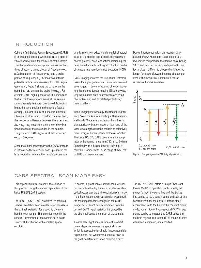
Coherent Anti-Stokes Raman Spectroscopy (CARS) is an imaging technique which looks at the specific vibrational motion in the molecules of the sample. This third-order nonlinear optical process involves three photons: a pump photon of frequency ωP, a Stokes photon of frequency ωS and a probe photon at frequency ωPr. At least two intense pulsed laser lines are necessary for CARS signal generation; Figure 1 shows the case when the pump line (ωP) acts as the probe line (ωPr). For efficient CARS signal generation, it is important that all the three photons arrive at the sample simultaneously (temporal overlap) while imping-ing at the same position in the sample (spatial overlap). In order to look at a specific molecular vibration, in other words, a certain chemical bond, the frequency difference between the laser lines Δω = ωP – ωS needs to match one of the vibra-tional modes of the molecules in the sample. The generated CARS signal is at the frequency ωCARS = 2ωP – ωS.

Since the signal generated via the CARS process is intrinsic to the molecular bonds present in the laser excitation volume, the sample preparation

This application letter presents the solution to this problem using the unique capabilities of the Leica TCS SP8 CARS system.

The Leica TCS SP8 CARS allows you to acquire a spectral excitation scan in order to rapidly assess the optimal excitation for a specific chemical bond in your sample. This provides not only the spectral information of the sample but also its structural distribution with excellent spatial resolution.

INTRODUCTION

CARS SPECTRAL SCAN MADE EASY

time is almost non-existent and the original natural state of the sample is preserved. Being a multi- photon process, excellent optical sectioning can be achieved and efficient signal collection can be obtained using non-descanned detectors (NDD).

CARS imaging involves the use of near infrared lasers for signal generation. This offers two-fold advantages: (1) Lower scattering of longer wave-lengths enables deeper imaging (2) Longer wave-lengths minimize auto-fluorescence and avoid photo-bleaching and its related photo-toxic/ thermal effects.

In this imaging methodology, the frequency differ-ence Δω is the key for detecting different chem-ical bonds. Since every molecular bond has its characteristic vibration mode, at least one of the laser wavelengths must be variable to selectively detect a signal from a specific molecular vibration. The Leica TCS SP8 CARS uses a tunable pump laser with a tuning range from 780 nm to 940 nm. Combined with a Stokes laser at 1064 nm, it covers all Raman shifts in the range of 1250 cm-1 to 3400 cm-1 wavenumbers.

Of course, a quantifiable spectral scan requires not only a tunable light source but also constant optical power over the entire excitation scan range. If the illumination power varies with wavelength, the resulting intensity changes in the CARS image stack cannot be discriminated from the desired CARS signal variation introduced by the chemical/spectral contrast of the sample.

Tunable laser light sources inherently exhibit power dependence over the spectral range, which is acceptable for simple image acquisition experiments. But whenever a spectral scan is the goal, constant excitation power is a must.

Due to interference with non-resonant back-ground, the CARS spectral peak is generally red-shifted compared to the Raman peak (Cheng 2007) and this shift is sample-dependent. This fact makes it difficult to choose the right wave-length for straightforward imaging of a sample, even if the theoretical Raman shift for the respective bond is available.

The TCS SP8 CARS offers a unique “Constant Power Mode” of operation. In this mode, the power for both the pump line and the Stokes line can be set to a certain value and kept at this constant level for the entire “Lambda-stack” experiment. With the help of the constant power mode, acquisition of hyper-spectral CARS image stacks can be automated and CARS spectra in multiple regions of interest (ROIs) can be directly visualized, compared, and exported.

V1, V2: virtual state

Ener

gy

P S Pr CARS

V2V1

S1

S0

ω ω ω ω

S0,: ground stateS1,: excited state

Figure 1: Energy diagram for CARS signal generation.

4

Choose the right objectiveCARS imaging needs two near infrared wavelengths impinging on the sample simultaneously. Any chromatic aberration will lead to a mismatch of the two PSFs (Point Spread Functions) and the signal generation will fail. Therefore, objectives with optimal chromatic correction for wave-

This application letter shows how to conduct CARS spectral analysis with the Leica TCS SP8 CARS. The following sections describe the software user interface while providing tips and tricks to extract the most out of your system.

Note:If the CARS laser is tuned to a wavelength which generates CARS signals in the range outside of the current filter cube, a pop-up display (see Figure 2) informs the user that the filter cube has to be changed and waits for user confirmation.

This dialog could also show up during a spectral scan. If you define a scan range across the 2000 cm-1 marker, the system will stop the data acquisition until the filter cube has been changed and confirmed. After that, the system

SYSTEM PREPARATION

lengths used here are essential for successful CARS imaging. Leica offers a series of IRAPO objectives, which have the best chromatic cor-rection and highest transmission for near infrared light. The HC PL IRAPO 40x/1.10 W CORR objec-tive is strongly recommended for CARS experi-ments. In addition to the excellent chromatic

correction you can achieve the best resolution with its high numerical aperture. If you need a bigger scan field, you can choose the HC PL APO 20x 0.75 Imm CS2, or the newly available HC PL APO 20x 0.75 CS2 dry objective.

Avoid any stray light The CARS signal is detected with highly sensi-tive non-descanned detectors (NDD). Any stray light will lead to image background.

Darken the room if possible. If the system is not equipped with a black chamber, cover the micro-scope with an opaque material.

Choose the right CARS filter setTwo filter sets can be chosen for CARS imaging, CARS1200 and CARS2000. The CARS1200 covers the Raman shift range of 1250-2000 cm-1 and the CARS2000 covers 2000-3450 cm-1.

continues to acquire images. However, it is strongly recommended not to set the scan range across the 2000 cm-1 marker: no matter how careful you are while changing the filter cubes, you cannot avoid disturbing the sample position. This is especially true if you are working with epi-CARS detection. The sample movement makes the data analysis and interpretation difficult. It is recommended that you take two scans on either side of 2000 cm-1 and link the data sets subsequently.

Figure 2: Information for changing the filter cube.

5

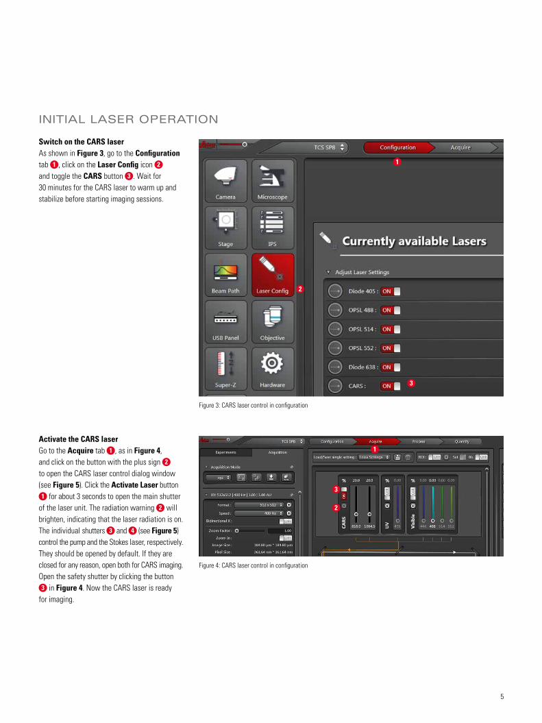
Switch on the CARS laser As shown in Figure 3, go to the Configuration tab 1 , click on the Laser Config icon 2 and toggle the CARS button 3 . Wait for 30 minutes for the CARS laser to warm up and stabilize before starting imaging sessions.

Activate the CARS laserGo to the Acquire tab 1 , as in Figure 4, and click on the button with the plus sign 2 to open the CARS laser control dialog window (see Figure 5). Click the Activate Laser button 1 for about 3 seconds to open the main shutter

of the laser unit. The radiation warning 2 will brighten, indicating that the laser radiation is on. The individual shutters 3 and 4 (see Figure 5) control the pump and the Stokes laser, respectively. They should be opened by default. If they are closed for any reason, open both for CARS imaging. Open the safety shutter by clicking the button 3 in Figure 4. Now the CARS laser is ready

for imaging.

INITIAL LASER OPERATION

Figure 3: CARS laser control in configuration

Figure 4: CARS laser control in configuration

1

1

2

3

3

2

6

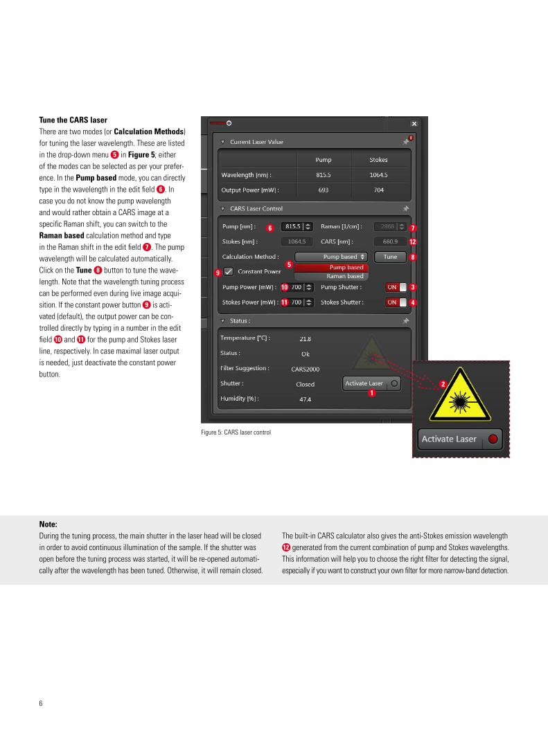
Tune the CARS laserThere are two modes (or Calculation Methods) for tuning the laser wavelength. These are listed in the drop-down menu 5 in Figure 5; either of the modes can be selected as per your prefer-ence. In the Pump based mode, you can directly type in the wavelength in the edit field 6 . In case you do not know the pump wavelength and would rather obtain a CARS image at a specific Raman shift, you can switch to the Raman based calculation method and type in the Raman shift in the edit field 7 . The pump wavelength will be calculated automatically. Click on the Tune 8 button to tune the wave-length. Note that the wavelength tuning process can be performed even during live image acqui-sition. If the constant power button 9 is acti-vated (default), the output power can be con-trolled directly by typing in a number in the edit field 10 and 11 for the pump and Stokes laser line, respectively. In case maximal laser output is needed, just deactivate the constant power button.

Figure 5: CARS laser control

6 7

5

4

3

8

21

9

Note: During the tuning process, the main shutter in the laser head will be closed in order to avoid continuous illumination of the sample. If the shutter was open before the tuning process was started, it will be re-opened automati-cally after the wavelength has been tuned. Otherwise, it will remain closed.

The built-in CARS calculator also gives the anti-Stokes emission wavelength 12 generated from the current combination of pump and Stokes wavelengths. This information will help you to choose the right filter for detecting the signal, especially if you want to construct your own filter for more narrow-band detection.

12

10

11

7

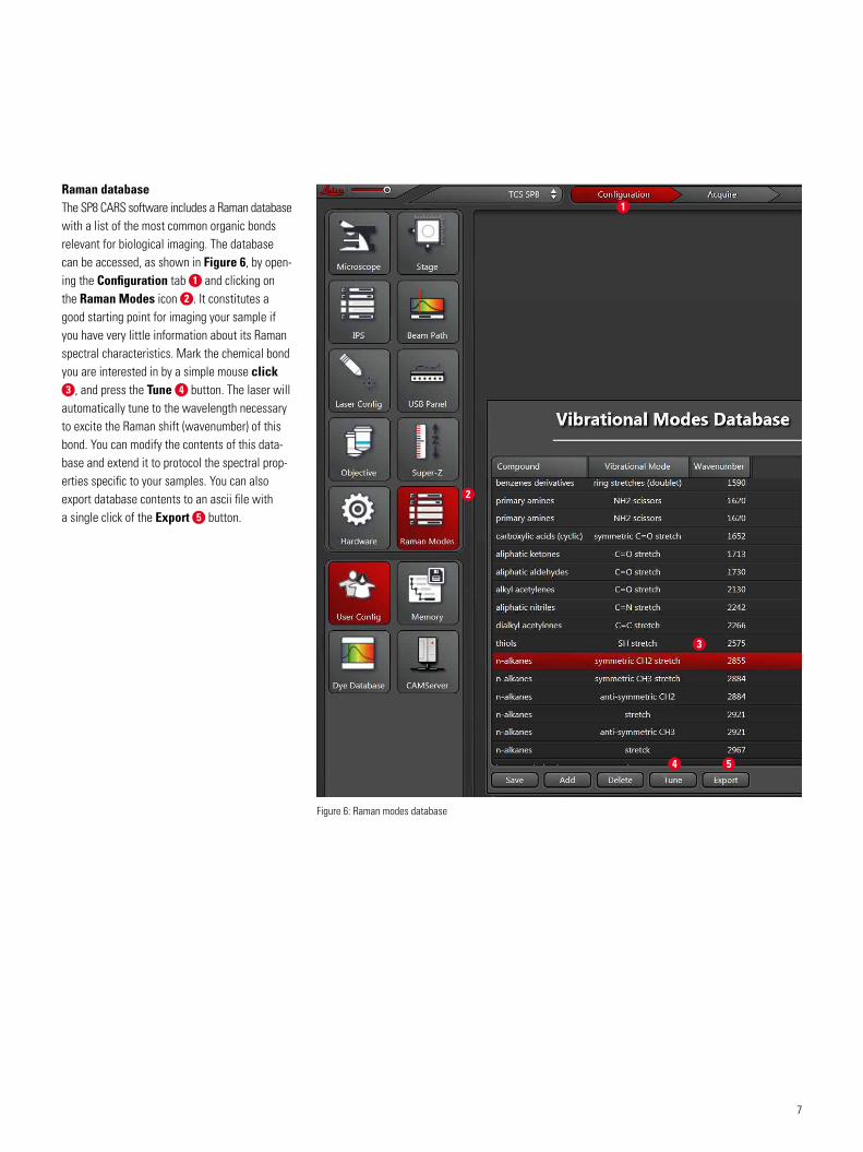
Raman database The SP8 CARS software includes a Raman database with a list of the most common organic bonds relevant for biological imaging. The database can be accessed, as shown in Figure 6, by open-ing the Configuration tab 1 and clicking on the Raman Modes icon 2 . It constitutes a good starting point for imaging your sample if you have very little information about its Raman spectral characteristics. Mark the chemical bond you are interested in by a simple mouse click 3 , and press the Tune 4 button. The laser will

automatically tune to the wavelength necessary to excite the Raman shift (wavenumber) of this bond. You can modify the contents of this data-base and extend it to protocol the spectral prop-erties specific to your samples. You can also export database contents to an ascii file with a single click of the Export 5 button.

Figure 6: Raman modes database

1

2

3

54

8

Detector activation Depending on the sample thickness you first need to decide whether to use TLD (Transmitted Light Non-Descanned Detector) or RLD (Reflected Light Non-Descanned Detector) for signal detec-tion. The propagation of the CARS signal is predominantly in the forward direction. If the sample is thin and transparent, it is always beneficial to use the TLD for “Forward CARS”.

1

2

3

54

1

3

2

4

In case you wish to investigate thick or scatter-ing samples, the RLD for “Epi CARS” will be the right detector choice.

Activate, as shown in Figure 7, F-CARS 1 for forward signal or Epi-CARS 2 for back- scattered signal. You can, of course, use both of them simultaneously, especially to check which detection mode is the best for your application.

Set the detector Gain 3 to 650 to 750 volts for optimum signal-to-noise ratio.

Start Live scan 4 . Increase the AOTF transmis-sion, as shown in Figure 8, for both pump 1 and Stokes 2 lasers until you get an image. The power adjustment can be combined with the control of output power under the constant power mode, see 9 in Figure 5.

Note: If using TLD detection, optimize the Koehler illumination. Make sure there are no additional or unnecessary filters in the beam path between sample and detector. The polarization filters in particular would block a huge part of the CARS signal. Also ensure that the aperture/iris diaphragm is fully opened. If working with the RLD detectors, ascertain that you have the right dichroic beam splitter in the fluorescence turret.

Caution: Since you are using highly sensitive non-descanned detection, please set AOTF for all visible and UV lasers to 0 and close the shutters 3 and 4 as in Figure 8. Stray light would otherwise cause an unwanted background signal that might swamp the CARS signal.

Figure 7: NDD control

Figure 8: AOTF for CARS laser power control

9

For a sample with unknown Raman spectral characteristics, a pre-scan with a large exci-tation wavelength step size (i.e. 1 nm) is strongly recommended.

In the Acquisition Mode 1 dropdown list in Figure 9, choose one of the lambda excitation scan modes 2 depending on your experimental requirements.

The dialog window for setting up a CARS excitation lambda scan (Figure 10) will be acti-vated. If your system has other tunable lasers, then choose CARS as the Light source 1 ; otherwise CARS will be chosen automatically.

Select the Pump based calculation mode or the Raman based calculation mode 2 for parame-ter setting. As you can switch between the two modes, the values for the Excitation Begin 3 and Excitation End 4 will be recalculated accordingly.

Constant power mode is activated by checking box 9 in Figure 5. Pump and Stokes laser lines are set separately with different values for constant power.

Check the image again with Live scan. Adjust the AOTF power or the detector gain if necessary.

After this step you can find out roughly the excitation wavelength at which the maximum signal from your sample appears; you can then optimize laser excitation power and PMT gain at this position.

No. of Excitation Steps 5 and Stepsize 6 are linked to each other; setting one of them would automatically modify the other based on the scan range. For easy workflow, it is recom-mended to set the step size yourself and let the system calculate the number of excitation steps. Note that the step size is in nanometers, irre-spective of the chosen calculation mode 2 . The smallest step size is 0.1 nm and the largest is 2 nm. After the definition of the step size and the number of steps, the end of the scan range will be slightly adjusted.

Start the data acquisition by just clicking the Start button (Figure 7 5 ). The scan will start at the shortest defined wavelength (or the largest Raman shift) and proceed to the longest wavelength. Note that the resulting spectral scan data is equi-spaced only in wavelength and not in wavenumber.

Note: For the constant power mode, set the value of the pump power below the minimum output power that is achievable in the entire tuning range of the chosen spectral scan.

Figure 9: Choose the CARS lambda scan mode

Figure 10: Set up the CARS lambda scan parameters

SET UP THE CARS EXCITATION PRE-SCAN

SET UP LAMBDA (Ʌ) SCAN

SET UP CONSTANT POWER MODE

1

3

1

5

4

2

6

2

10

CARS SPECTRAL SCAN ANALYSIS

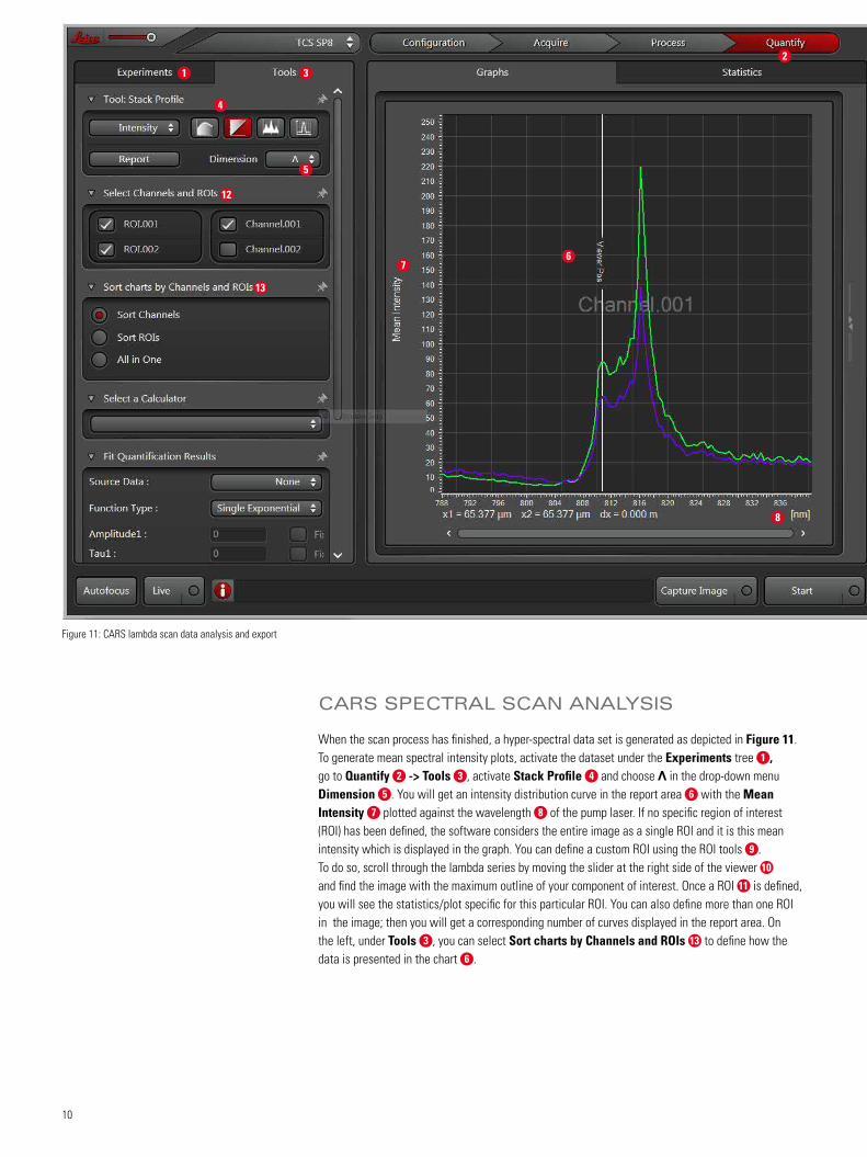
When the scan process has finished, a hyper-spectral data set is generated as depicted in Figure 11. To generate mean spectral intensity plots, activate the dataset under the Experiments tree 1 , go to Quantify 2 -> Tools 3 , activate Stack Profile 4 and choose Ʌ in the drop-down menu Dimension 5 . You will get an intensity distribution curve in the report area 6 with the Mean Intensity 7 plotted against the wavelength 8 of the pump laser. If no specific region of interest (ROI) has been defined, the software considers the entire image as a single ROI and it is this mean intensity which is displayed in the graph. You can define a custom ROI using the ROI tools 9 . To do so, scroll through the lambda series by moving the slider at the right side of the viewer 10 and find the image with the maximum outline of your component of interest. Once a ROI 11 is defined, you will see the statistics/plot specific for this particular ROI. You can also define more than one ROI in the image; then you will get a corresponding number of curves displayed in the report area. On the left, under Tools 3 , you can select Sort charts by Channels and ROIs 13 to define how the data is presented in the chart 6 .

Figure 11: CARS lambda scan data analysis and export

12

13

1 3

2

4

5

8

76

11

Figure 12: Export of spectral data for further analysis

As mentioned earlier, the curves displayed in the chart are the plot of the mean image intensity against the pump wavelength. But in the Raman literature, the commonly used term for describing CARS/Raman spectra is the Raman shift in wavenumber instead of pump wavelength. In order to convert to wavenumber, the data can be exported as an excel file.

To do so, activate the export function with a right mouse click in the chart area (see Figure 12) and choose Export 1 -> Excel 2 . The data will be exported in *.csv format which can be edited in spreadsheet applications.

To calculate the Raman shift from the pump wavelength, use the following formula with wavelengths in nanometers:

1

2

10

11

9

[ ]1 710)][

1][

1(=cmnmnm

RamanshiftSP

nmS 5.1064=

12

CARS SPECTRAL SCAN ACQUISITION

• Sample: Fresh chicken tendon tissue embedded in water

• Objective: HC PL IRAPO 40x/1.10 W CORR • CARS 2000/BP filter cube, CARS and SHG

channels acquired simultaneously• xyλ scan range: 2500-3300 cm-1

(787.8-840.7 nm) in 0.5 nm steps

In Figure 13, image A shows the CARS channel. The lipid droplets can be clearly recognized. Image B shows the SHG channel, where one can see the typical elongated and nicely orga-nized structure of collagen fibers in the tendon tissue. In the overlay image C, one can see how the lipid droplets are embedded among the collagen fibrils.

For quantitative analysis two ROIs are drawn, one enclosing a lipid droplet (green) and a sec-ond enclosing collagen protein fiber (violet). The related intensity and wavelength information is exported and re-plotted against the pump wave-length (top axis) and the Raman shift (bottom axis). Diagram D shows the data from the CARS channel where the green curve corresponds to the lipid area and the violet to the protein fibers. The lipid droplet exhibits a much stronger CARS signal (with a peak intensity of 240 gray values) than the protein area. In the lipid area, typical signal peaks for CH (2853 cm-1, white arrow) and CH3 (2936 cm-1, black arrow) can be observed; the CH bond signal is 2.5 times stronger. Within the protein fiber, one can observe these peaks as well, but with an overall lower intensity and, more importantly, with an inverted ratio of CH and CH3 signals. CH3 is now stronger than the CH signal. There is a much greater amount of

CH in lipid than in protein. Additionally, we see an increasing signal in the protein area starting from a Raman shift of approximately 3000 cm-1; this signal corresponds to water.

Image E shows the signal distribution of the same ROIs from the SHG channel. Clearly, there is no dependence between the signal intensity and the laser wavelength. No dominant peaks are observed either in the lipid area or in the protein area. However, the protein area in this channel has a much stronger signal (90–140 gray values) than the lipid area (around 20 gray values). This is a result of parallel organization of the collagen fibers in the tendon, which generates stronger SHG signals. In contrast, SHG signals are weak within the lipid droplets due to the absence of non-centro-symmetry, a pre-condition for efficient second-harmonic generation.

EXAMPLE FOR CARS SPECTRAL SCAN

After the pre-scan, the approximate maximum signal position can be localized. The optimum parameter settings, including AOTF values for the excitation power and PMT gain for the detection amplification, can be adjusted for the fine spectral scan of CARS images.

Keeping all other parameters as before, adjust the excitation step size according to the required spectral resolution for the final lambda scan. Data acquisition can now be started by simply clicking the Start button.

The spectral scan can also be combined with XZ or XYZ (3D acquisition) or XYT (time experiment) by choosing the appropriate mode of acquisition shown in Figure 9.

13

250

200

150

100

50

0

25

837.

7

832.

7

827.

7

822.

7

817.

7

812.

7

807.

7

802.

7

797.

8

792.

8

787.

8

2543

2615

2687

2761

2835

2910

2986

3063

3141

3220

3300

20

15

10

5

0

pump wave length (nm)

inte

nsity

(AU)

Raman shift (cm-1)

lipid

protein

200

160

120

80

40

0

200

837.

7

832.

7

827.

7

822.

7

817.

7

812.

7

807.

7

802.

7

797.

8

792.

8

787.

8

2543

2615

2687

2761

2835

2910

2986

3063

3141

3220

3300

160

120

80

40

0

pump wave length (nm)

inte

nsity

(AU)

Raman shift (cm-1)

lipid

protein

Figure 13: CARS spectral analysis of chicken tendon.

References:Cheng JX 2007, Coherent anti-Stokes Raman scattering microscopy. Appl Sectrosc. 61(9):197-208Evans CL, Xie XS 2008, Coherent anti-stokes Raman scattering microscopy: chemical imaging for biology and medicine. Annu Rev Anal Chem, 1:883-909

250

200

150

100

50

0

25

837.

7

832.

7

827.

7

822.

7

817.

7

812.

7

807.

7

802.

7

797.

8

792.

8

787.

8

2543

2615

2687

2761

2835

2910

2986

3063

3141

3220

3300

20

15

10

5

0

pump wave length (nm)

inte

nsity

(AU)

Raman shift (cm-1)

lipid

protein

200

160

120

80

40

0

200

837.

7

832.

7

827.

7

822.

7

817.

7

812.

7

807.

7

802.

7

797.

8

792.

8

787.

8

2543

2615

2687

2761

2835

2910

2986

3063

3141

3220

3300

160

120

80

40

0

pump wave length (nm)

inte

nsity

(AU)

Raman shift (cm-1)

lipid

protein

A D

E

B

C

14

NOTES

15

NOTES

5/16

· Or

der n

o.: 1

5931

0403

8 · ©

201

6 by

Lei

ca M

icro

syst

ems

CMS

GmbH

.Su

bjec

t to

mod

ifica

tions

. LEI

CA a

nd th

e Le

ica

Logo

are

regi

ster

ed tr

adem

arks

of L

eica

Mic

rosy

stem

s IR

Gm

bH

Leica Microsystems CMS GmbH

Am Friedensplatz 3 · 68165 Mannheim, Germany · T +49 621 70280 · F +49 621 7028 1180

www.leica-microsystems.de

CONNECT WITH US!