carine_31_us
TRANSCRIPT

������������� ������������������������� � �for Microsoft Windows!
1989-1998 C. Boudias & D. Monceau
User's Guide

Version 3.1 user manual by C. Boudias and D. Monceau ©1998. Version 3.0user manual was translated from the French by K'TO Manning and D.Monceau©1996. Original user manual of version 3.0 ©1994 C. Boudias and D.Monceau.
The software CaRIne Crystallography version 3.0 for Macintosh has beenconceived, realized and edited by C. Boudias and D. Monceau ©1994.
CaRIne Crystallography version 3.0 has been adapted from the Macintoshversion to MS-Windows by C. Boudias with the help of Y. Breton ©1996.Version 3.1 by C. Boudias and D. Monceau ©1998.
Information in this document is subject to change without notice. Companies,names, and data used in examples herein are dictitious unless noted. No part ofthis document should be reproduced or transmitted in any form by any means,electronic or mechanical ones, for any purpose, without express writtenpermission of the authors.
Macintosh™ is a registered trademark of Apple Computer, Inc.Apple ® and the Apple logo are trademarks of Apple Computer Inc.IBM is a registered trademark of International Business Machine.WINDOWS, MS DOS and Word are trademarks of Microsoft Corporation.Mac Draw and Mac Write are trademarks of Claris Corporation.
User manual last review : January 1998
© 1989-1998 Cyrille Boudias and Daniel Monceau. All rights reserved.

Table of contents T-1
TABLE OFCONTENTS T
Table of contents ..........................................................................T-1
Introduction ..................................................................................I-1
Chapter 0 :Installation Procedure...................................................................0-1
0.1 Before Installation..........................................................................0-1
System Requirements.....................................................................0-2
0.2 Installation.....................................................................................0-3
0.2.1 Installation procedure...............................................................0-3
0.2.2 Install on a network..................................................................0-4
0.2.3 File compatibilities...................................................................0-4
0.3 Files and directories.......................................................................0-5
0.3.1 Data base directories................................................................0-5
0.3.2 Import-Export directory............................................................0-5
0.3.3 Personal directory.....................................................................0-5
0.3.4 How to stay in the current directory..........................................0-5

Table of contents T-2
0.3.5 Drag & drop CEL and CRY files..............................................0-5
Chapter 1 :CaRIne and the crystallography ..................................................1-1
1.1 Notions of unit cell, lattice, lattice points, motif, crystal.................1-1
1.2 Crystalline systems, Bravais lattices, Space Groups........................1-2
1.3 Indices of directions and planes......................................................1-4
1.4 Use of CaRIne in 2D......................................................................1-5
1.5 Defects in crystals..........................................................................1-6
1.6 Units employed..............................................................................1-7
Chapter 2 :General description of CaRIne.....................................................2-1
2.1 The different types of windows.......................................................2-1
The "Crystal" windows..................................................................2-1
The status bar................................................................................2-2
The "Stereographic projection" windows........................................2-3
The "Reciprocal lattice" windows...................................................2-4
The "XRD" windows.....................................................................2-4
The "Tool palettes" Windows.........................................................2-5
Context menus...............................................................................2-5
2.2 ? Menu...........................................................................................2-6
2.3 Files Menu.....................................................................................2-7
2.4 Edit Menu ...................................................................................2-12

Table of contents T-3
2.5 Cells Menu...................................................................................2-13
2.6 (hkl)/[uvw] Menu.........................................................................2-15
2.7 Calcul. Menu...............................................................................2-20
2.8 Specials Menu.............................................................................2-29
2.9 Crystal Menu ..............................................................................2-36
2.10 View Menu...................................................................................2-46
2.11 Windows Menu............................................................................2-49
Chapter 3 :Selection of a crystalline structure ...............................................3-1
3.1 Loading a motif, a unit cell or a crystal from the libraries...............3-1
3.2 Use of Bravais' lattices...................................................................3-2
3.3 Construction of a new unit cell.......................................................3-4
3.4 Space groups, construction of a new motif......................................3-9
3.5 Use of Mendeleev's table (Periodic table of the elements)..............3-11
Chapter 4 :Visualisation functions..................................................................4-1
4.1 The different reference frames of CaRIne.......................................4-1
4.2 Rotations........................................................................................4-2
4.2.1 Using Miller indices.................................................................4-2
4.2.2 Using the keyboard...................................................................4-2
4.2.3 Using the mouse.......................................................................4-3
4.2.4 Using the stereographic projection............................................4-4
Table of contents T-4
4.2.5 Using the Rotations tool palette................................................4-4
4.3 Scales.............................................................................................4-4
4.4 Planes translations.........................................................................4-5
4.5 The "Graphics" command.............................................................4-5
For a Crystal window.....................................................................4-5
For a Stereographic projection window...........................................4.8
For a Reciprocal lattice window......................................................4.9
For a XRD window......................................................................4.10
Chapter 5 :Lattice associations .......................................................................5-1
5.1 "Matrix-Precipitates" type association............................................5-1
5.2 Association with "Relation of Epitaxy"...........................................5-4
5.3 Orientating a group of lattices by giving several relations of epitaxy5-6
Chapter 6 :The stereographic projections ......................................................6-1
6.1 Introduction...................................................................................6-1
6.2 Specials/Stereo. Proj. Menu...........................................................6-2
6.3 Orientate the stereographic projection............................................6-9
6.4 View Menu...................................................................................6-10

Table of contents T-5
Chapter 7 :The X-Rays diffraction patterns for randomorientated powders .......................................................................7-1
7.1 Introduction : Calculation of peak intensities..................................7-1
7.2 Special/XRD (powder) Menu.........................................................7-4
7.3 View Menu.....................................................................................7-9
Change XRD scales with mouse...................................................7-10
Chapter 8 :The reciprocal lattices...................................................................8-1
8.1 Introduction...................................................................................8-1
Structure factor calculations...........................................................8-2
Some geometric relationships.........................................................8-4
8.2 Specials/Reciprocal Lattice Menu.................................................8-6
8.3 View Menu.....................................................................................8-8
Chapter 9 :CaRIne in examples ......................................................................9-1
9.1 Indexing of a diffraction pattern.....................................................9-1
9.2 Standard projections of a cubic crystal............................................9-4
9.3 ABCABC… sequence in FCC and ABAB… sequence in HCP.......9-6
9.4 Visualisation of the (111) surface of diamond.................................9-8
9.5 X-Rays diffraction : Au-Cu alloys.................................................9-10
Table of contents T-6
Appendix A :Format Standard ASCII File and Format of DOS version files A-1
A-1 The "Cell Standard ASCII File"....................................................A-1
The different colour reference.......................................................A-2
Unit cell described from the space group.......................................A-3
A-2 The "Crystal Standard ASCII File"................................................A-4
A-3 The "Cell DOS File Format".........................................................A-7
A-4 The "Crystal DOS File Format".....................................................A.8
Appendix B :Setting default values with the registry.......................................B-1
Modification of the registry...........................................................B-1
Details of the registry....................................................................B-6
Appendix C :Diffusion factors for the atoms/ions ............................................C-1
Appendix D :How to use list generators............................................................D-1
Index...............................................................................................i-1

Introduction I-1
INTRODUCTION
asic crystallography will often appear as an obvious subject for...crystallographers! But every teacher had seen some students fightingwith 3D representations and having troubles to understand the meaning
of a stereographic projection from a drawing on the blackboard. The teacherwill often have troubles to teach what seems to be a geometrical evidence.
The first purpose of CaRIne was to help the non-specialist to visualize 3D-structures (cells, planes, directions...). The "computer tool" was chosen becauseof its capacities to access to the third dimension through rotations. It was alsopreferred to ball & stick models because of its versatility and interactivequalities.
In June 89, CaRIne was born and able to draw every structures, simple ones andcomplex ones, thanks to a good mathematical background. The early success ofCaRIne in France brought to the authors many comments and suggestions, andthe software evoluated from versions 1.0 to version 2.5.
In 93, the idea had come to extend the software to other representations, usingthe new possibilities of computers interactivity and ease to use. Version 3.0 wasconceived in September and one year later it began to be distributed for Macand in French only.
This new local success has encouraged the authors to bring the software to themore popular Microsoft Windows environment. Since 89 CaRIne has evoluatedto become an useful tool for teaching and now also for edition and research.With this new English translation, we hope that our work will help numerouspersons all around the world in their everyday work.
Waiting for your feedback,
the authors.
B

Introduction I-2
Note :
We don't think it is necessary to read all the user manual in details before tostart. But, after a first contact with the software, we encouraged the user to readchapters 1 and introductions of chapters 6, 7 and 8, which explain the"philosophy" of this work. Then, you can exercise with chapter 9. To get somehelp on a precise function you will reference to chapter 2 for the real lattice, 6for the stereographic projection, 7 for the X-Rays Diffraction, 8 for thereciprocal lattice. You can also have a fast general look to the manual to knowwhat it is possible to do, and you will find a lot of pictures !
It is now time to wish you "bon voyage".
Many thanks to :
Denis Ansel, Sam et Jean Blachère, Bernadette Baroux, Sophie et PascalBartek, Gérard Béranger, Dagmara Berztiss, Nicolas Boëns, GuillaumeBoucher, Sandrine Boudias, Bernadette et Bernard Boudias, Yves Breton,Sophie Bruges, Philippe Buffat, Françoise Cabané, Daniel Cabrol, Rémi Capet,Kay Chhor, Michel Clavel, Alain Dautant, Frank Elstner, Philippe Buffat, YvesFranchot, Yvan Guillot, Alain Hewat, Julitte Huez, Timothy Klemmer, KateKrenell, Alina Klimczyk, Jean Laugier, K'TO Manning, Claudine et BernardMonceau, Claude Monty, Georgette Petot-Ervas, Claude Petot, Jean Philibert,Claude Pommier, Laurence Pouchenot, Jean-Pierre Rabine, Bill Soffa, Mr T...
Installation Procedure 0-1
CHAPTER 0Installation Procedure 0
This Chapter is dedicated to the installationprocedure of CaRIne.
0.1 Before Installation
Before installing CaRIne 3.1, you should check the following points :
• Have a look at the "readme.txt" file, located on the install disk orCD-ROM. This file contains information which couldn't be writtenin time on the user manual. It can be opened with any wordprocessor (Notepad or WordPad for example);
• Make a copy of your installation floppy; • Fill in and send the registration card, in order to get full technical
assistance and to be informed of the new versions coming out at thebest price.

Installation Procedure 0-2
System Requirements :
CaRIne 3.1 requires the following minimum configuration :
• An IBM Personal Computer, or 100 percent compatible, runningMicrosoft Windows 95/NT4.0 or higher.
• An 486 or higher processor. • Height megabytes of available memory (8MB RAM). • A 1.44-MB, 3.5-inch disk drive or CD-ROM. • 20 free MB on the hard disk drive.

Installation Procedure 0-3
0.2 Installation
0.2.1 Install procedure
The Setup program provided by CaRIne Crystallography performs alltasks necessary for installing the CaRIne components. You can installeverything at once or install just a subset and upgrade it later withadditional libraries, samples, help files, or other components.
To run Setup :
1. Place Disk 1 in drive A (or B...) or CD-ROM. 2. From the control panel select Add/Remove programs menu and type
A:\Setup in the command line box. 3. Install prompts you with a dialog box that describes the program and
lets you continue or exit. 4. Follow the installation instructions.
When the installation procedure is ended, Setup add CaRIne 3.1 in theStart Menu :
To run the CaRIne 3.1 program, select it on the Start menu.
To select the language of CaRIne, choose File|Options. It is possible toswitch between French and English while the program is running.

Installation Procedure 0-4
0.2.2 Install on a network
When following the install procedure (given in 0.2.1), the libraries willbe automatically placed in the same directory as the CaRIne v3.1program.As a consequence, users without writing rights on the network serverdisks will not be able to save their own files in the default directories.To solve this problem, a new default folder has been created : Personaldirectory which needs to be setup by every network user (see 0.3.3).
0.2.3 File Compatibilities
Note : CaRIne v3.1 is able to read your 3.0 version files, but version 3.0will not read v3.1 files ! If you really need to go back from v3.1 to v3.0,you may use the ASCII files (ACE and ACR) which are fullycompatibles (even with the Mac version).
As a 32 bits windows application, CaRIne v3.1 allows 255 character filenames.
Icons have been changed in order to differentiate version 3.0 and 3.1cells and crystals files.
: for cell files (extension CEL)
: for crystal files (extension CRY)
Installation Procedure 0-5
0.3 Files and directories
0.3.1 Data Base directories
When following the install procedure (given in 0.2.1), the libraries willbe automatically placed in the same directory as the CaRIne 3.1program. In order to have a quick access to these files, CaRIne proposesto associate them with directories. To set all the associated directories,select the function File | Options.
0.3.2 Import-Export directory
A new default directory has been added in version 3.1 : «Import-Export».It concerns all the text files created by CaRIne (angle list, X-Raydiffraction list, ...). Use the File|Options function to set this directory.
0.3.3 Personal directory
In case you need to load/save your files all in the same directory, CaRIneoffers you the possibility to define a personal directory. This function isespecially useful in case of a network utilization. To select your personaldirectory call the File/Option function, define your folder and check thebox "use the personal directory"
0.3.4 How to stay in the current directory
When loading or saving several files, it is now possible to stay in thesame directory. To do so, press on the Alt key when loading or saving afile (File|Load or Save).
0.3.5 Drag and drop CEL and CRY files
In order to facilitate the loading and saving of CEL and CRY files, it isnow possible to select these files from the Explorer and to «drag anddrop» them onto the CaRIne application.

Installation Procedure 0-6

CaRIne and the crystallography 1-1
CHAPTER 1CaRIne and the crystallography 1
This chapter describes how different crystallographicconcepts are approached and interpreted by thesoftware.
1.1 Notions of unit cell, lattice, lattice points, motif,crystal,...
Lattice / Lattice points :
The lattice is classically defined as a group of points organised in space in sucha way that each point has the same environment.
Motif :
The motif is the minimal unit which is repeated in the lattice.
Unit cell :
The unit cell is the volume defined by the lattice vectors a, b and c. It is theminimal unit of volume which allows the construction of the total volume byunit cell juxtaposition (lattice translations).
Crystal :
CaRIne software interprets "crystals" as being all information which allows theconstruction of a complete representation.The following table clarifies this point by describing what is contained in eachobject corresponding to crystallographic concepts :

CaRIne and the crystallography 1-2
Motif • the list of non-equivalent atoms
Unit cell • the list of all atoms found in the volume (a,b,c)• the cell parameters (which define the system)
Crystal• the unit cell as above• the number of cells following the directions of a, band c• all modifications applied to the atoms(displacement, substitution, vacancy, interstitial,…)leading to a non-respect of lattice translations.
Table 1.1 : Motif, Unit cell and Crystal
The following paragraph explains how CaRIne passes from one object toanother.
1.2 Crystalline systems, Bravais' lattices, Space Groups
When cell parameters a, b, c, α, β, γ, are set, one of the 7 crystalline systemsis selected, which appears in the status bar, at the bottom of the window.
The choice of system can also be made by selecting a Bravais' Lattice . Inwhich case the choice of system from the Cell Menu is followed by the choiceof mode from the corresponding sub-menu (primitive, body-centred, basecentred, face-centred).
CaRIne then opens a dialogue-box which allows the modification of the cellparameters (respecting the system) and a sphere is assigned to each point of thelattice. Obviously this sphere can be considered as an atom, and assigned achemical symbol using Mendeleev's Periodic Table, which is available.However, this is not required, the spheres can also be assimilated to simplelattice points.

CaRIne and the crystallography 1-3
At this point, it would be preferable to be able to substitute a motif at eachlattice point, and this function will be developed in a future version of CaRInein which the lattice points and the atoms will be clearly distinguished. At themoment, this substitution can be made by using space groups. The choice of agroup leads to a dialogue-box where the position of non-equivalent sites areentered. This defines a motif which will be repeated according to the group'selements of symmetry. There is therefore no obligation to place an atom at0,0,0, for example.
e.g. : It is possible to choose the group 225 (Fm3m) and to enter a one-atommotif, placed at 1/2,0,0. The face centred cubic lattice is present but shiftedfrom the origin.
The space group is the combination of all the possible transformations ofsymmetry in a crystalline structure. The space group characterises thesymmetry of a crystalline structure in the same way that a point groupcharacterises the symmetry of the exterior form of the crystal and the symmetryof its macroscopic properties. There are 32 point groups of symmetry (32crystalline classes).
Each point group corresponds to several space groups. From the space group,the point group is obtained by eliminating all the translations. On the otherhand, space groups can be deduced from the point groups. In order to do this,an examination of all the possible combinations between the symmetryelements of the point group and the translations of the type of lattice allowed bythe point group is necessary.
230 space groups can be obtained. Each is a group in the mathematical sense ofthe word.

CaRIne and the crystallography 1-4
crystal (no longer respecting the lattice translations)
Choice of
corre
sponding sp
ace gr
oup (if
a motif
is requ
ired a
t each
point of
lattice
)
An atom placed at each point of the
lattice
Calculation of positions
Calculation of translationsfollowing a,b and c
Modifications (crystalline defect)
motif+ space group
+ cell parameters (system)
Transfo
rmati
on of
a cry
stal to
a cel
l
crystal
Unit cell
Bravais's lattice
entry
entry
entry
Fig 1.2 : Concept of creation of Motifs, Cells, Lattices and Crystals
1.3 Indexes of directions and planes
• To locate a crystallographic direction duvw or a row of atoms, the indicesu, v and w are used. They are defined as follows:
duvw = u.a + v.b + w.cwhere a, b et c are vectors of the unit cell and u, v, w are positive integers.

CaRIne and the crystallography 1-5
• For the planes, Miller's indices are used. For the family of planes {hkl},the first plane intersects the axes xx', yy', zz' at a/h, b/k and c/l when a, band c are cell parameters.
• Conversion 3 ➯ 4 indices (hexagonal system):
duvw ➯ dUVTW with
U =1
3⋅ 2⋅ u − v( ), V =
1
32 ⋅ v − u( ), T = − U + V( )et W = w
dhkl ➯ dHKTL with H = h, K = k, T = −h − l et L = l
1.4 Use of CaRIne in 2D
In order to introduce the concept of punctual defects or elements ofsymmetry easily, a teacher may wish to work in two dimensions (2D). Thisis possible with CaRIne. The procedure is as following :
1 - define the parameters of the 2D cell : a, b and γ
2 - define the cell, with the atomic coordinate z placed at 0
3 - project in the direction perpendicular to the plane (001)
4 - Extend the lattice following a, b and c, with the required values of na andnc and especially nc=0
To carry out this sequence, see the description of the necessary functions inchapter two.
The second way to proceed is to work in a plane (hkl) (see the function :Selection of a plane (hkl), chap. .2). Once the plane has been selected, projectperpendicularly to this plane, selecting only the atoms of the plane (hkl) in thegraphic options (see chapter 4, command "Graphics").

CaRIne and the crystallography 1-6
1.5 Defects in crystals
The following table presents the functions made available by CaRIne, in orderto represent crystalline defects.
Defect dimension Kind of defect Functions to use
dimension = 0 substitutionnal atom Menu Crystal, modify atom, orMenu Cell, creation
vacancy Menu Crystal, vacancy
relaxation (move atoms) Menu Crystal, modify atom
interstitial atom Menu Crystal, add atom
Frenkel and Schottky defectsMenu Crystal, modify atom, orMenu Crystal, add atom
dimension = 1 dislocations Menu Crystal, modify atom in orderto move the concerned atom one byone !
dimension = 2 twin boundary Menu Special, relation of epitaxy,or Associated lattices :
grains boundary just to study the orientationrelationships between crystals.
dimension = 3 precipitate
Table 1.3 : Defects in crystals
CaRIne possesses all the necessary functions for the creation of point defects.Future versions will include tools aimed at facilitating the representation ofdislocations.

CaRIne and the crystallography 1-7
1.6 Units employed
The units of the International System are used, except in the case of atomicradii and sizes linked to them, where the Angstrom is preferred to thenanometer. The Angstrom is a unit which is coherent with the InternationalSystem (1Å=10-10m). Moreover, the unit is widely used in crystallographybecause it is close to an atomic diameter, and also because it appears in thetables of interplanar distances of the JCPDS (Joint Committee for PowderDiffraction Standards).
Physical Variable Unit Symbol Remarksatomic radius Angstroms Åreduced atomic coordinates without unit between 0 and 1oxidation degree without unitoccupation factor without unit between 0 and 1cell parameters: a, b and c Angstroms Å same unit than the atomic radiicell parameters: α, β, and γ degrees °spread of lattice: na, nb and nc without unit integers positives or nilcrystallographic direction u,v,w without unit integers positives or nilcrystallographic plane h,k,l without unit integers positives or nil"thickness" of a plane: ε without unit real between 0 and 0.5distance between atoms Angstroms Å same unit as a, b and catomic coordonnates in the cellreference frame a,b,c
without unit real positive or nil
angles between directions andplanes
degrees °
cell volume V cubic Angstroms Å3 unit consistent with a, b and c
cell density without unit real between 0 and 1wave length of X-rays: λ Angstroms Å XRD and interplanar distances listinterplanar distance dhkl Angstroms Å
sum of squared indices: Σind2 without unit interplanar distances list
Bragg angle: θ degrees ° interplanar distances liststructure factor: Fhkl without unit interplanar distances list
multiplicity: p without unit interplanar distances list, integer > 0relative intensity of a peak: I% without unit 0-100% XRD and interplanar distances listaccelerating voltage: V kilo-Volts kV identification of planes
electrons wave-length e-: λ Angstroms Å identification of planes
camera length: L centimetres cm identification of planescamera constant: K cm.Å identification of planesdistances on diffraction patterns: r1and r2
centimetres cm.Å identification of planes
zone axis without unit cf. uvwPhysical Variable Unit Symbol Remarks
solid angle: S.A.% without unit 0-100% shells

CaRIne and the crystallography 1-8
number of atoms in a layer: nb without unit shells, integer positive or niltemperature factor squared
AngstromsÅ2 XRD, real between 0 and 20 (or more)
poles without unit stereographic projection , cf. hkltraces without unit stereographic projection, cf. hklangles θ and φ degrees ° stereographic projectionlinks thickness without unit integer between 0 and 10 (or more)size of shading zone pixel integer between 0 and 50 (or more)intensity variation percent % shading due to depht
Table 1.4 : Units employed
General description of CaRIne 2-1
CHAPTER 2General description of CaRIne 2
This chapter describes the different types of windowsmanaged by CaRIne and the commands which areassociated with them.
2.1 The different types of windows
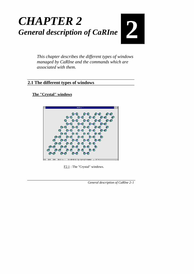
The "Crystal" windows
F2.1 : The "Crystal" windows.

General description of CaRIne 2-2
The "crystal" windows allow the visualisation of your crystal structures.Their size can be modified, the lattice is always centred in its window. Thefunction associated with "real lattice" windows are described throughout thischapter. At the bottom of such a window, a status bar which gives the angleof view, the current command and the cell parameters,.... can be found.
The status bar
The status bar is composed of 4 sections. In order to change the sections,click on the status bar. Each section is composed of angles which define theangle of view and the command associated with the lattice at the time.
A command can be selected from a menu, using the mouse, thecorresponding short key or by using the tool palettes. This command isshown in the status bar and remains active until another command has beenselected.
- Information on the cell :
View Angle
Number of positions in the motif Space group
Crystalline sytemCell parametersCommand associated with the lattice
- Information on the crystal :
View Angle
Number of atoms and l inks in the crystal
General scale
Command associated with the lattice
Radii scale
Spread of crystal

General description of CaRIne 2-3
- Information on planes and direction :
View angle Command associated with the lattice
Current planes Current direction
- Information on memory :
View angle Command associated with
the crystal
Size of crystal in bytes
Size of picture in bytes
The "Stereographic projection" windows
F2.2 : The "Stereographicprojection" window.
The "Stereographic projection"windows enables the visualisation of theStereographic projectionscorresponding to the active crystalwindow (see Chap. 6). The size of thestereographic projection automaticallyadapts itself to that of the window.There is only one window of this typefor each crystal. The associatedcommands are situated in theSpecial/Stereo. Proj. Menu.
At the bottom of each "stereographicprojection" window there is a status barwhere the angles corresponding to thepresent position of the protractor andthe associated command can be found.
The "reciprocal lattice" windows
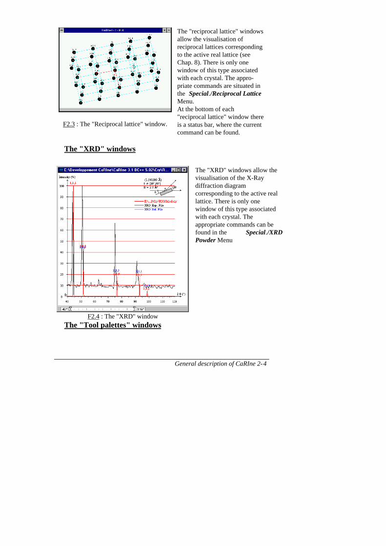
General description of CaRIne 2-4
F2.3 : The "Reciprocal lattice" window.
The "reciprocal lattice" windowsallow the visualisation ofreciprocal lattices correspondingto the active real lattice (seeChap. 8). There is only onewindow of this type associatedwith each crystal. The appro-priate commands are situated inthe Special./Reciprocal LatticeMenu.At the bottom of each"reciprocal lattice" window thereis a status bar, where the currentcommand can be found.
The "XRD" windows
F2.4 : The "XRD" window
The "XRD" windows allow thevisualisation of the X-Raydiffraction diagramcorresponding to the active reallattice. There is only onewindow of this type associatedwith each crystal. Theappropriate commands can befound in the Special./XRDPowder Menu
The "Tool palettes" windows
General description of CaRIne 2-5
CaRIne has three "tool palettes" which allow rapid access to the functions ofthe Crystal, Special and View Menus. These are floating windows (they arealways above the desktop of your computer) and can be hidden or activatedwith the help of the "…tools" functions from the Windows Menu.
In this manual, if an icon appears in front of a command (or a function) of amenu, access to it is available through one of the tool palettes.
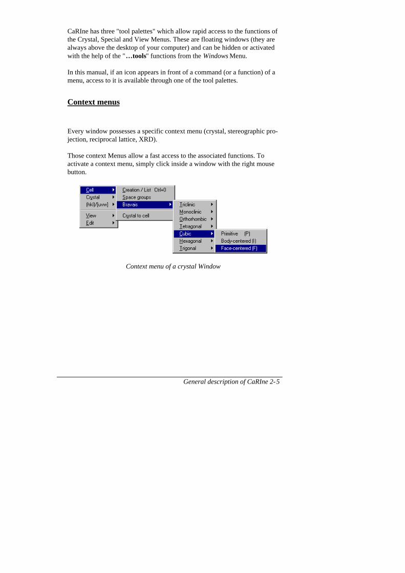
Context menus
Every window possesses a specific context menu (crystal, stereographic pro-jection, reciprocal lattice, XRD).
Those context Menus allow a fast access to the associated functions. Toactivate a context menu, simply click inside a window with the right mousebutton.
Context menu of a crystal Window

General description of CaRIne 2-6
2.2 ? Menu
About CaRIne...
This function allows you to find rapidly the addresses of both authors anddistributor, as well as information concerning the copyrights.
F2.5 : About CaRIne.

General description of CaRIne 2-7
2.3 Files Menu
The functions of the Files Menu permit the management of your documentfiles. There are 3 sorts of files :
• Motif or Cells (CEL, MTF2, MTF*)• Crystals (CRY, RES2, RES*)• Pictures (WMF, PICT)
CaRIne allows several crystal files of the same unit cell to be saved. In orderto differentiate these files, CaRIne automatically gives the extension ".cel" tothe motif files and ".cry" to the crystal files (see Chap.3)
CaRIne also manages the importation and exportation of motifs and latticesfrom the ASCII files ("text" format).
New Ctrl- N
This command allows the creation of a new "crystal" window, a prop for therepresentation of a crystalline lattice. A new motif should be constructed(see Chap. 3) .
When a cell or a lattice is loaded from the data bases, a window isautomatically created without having to use this "New" function.
Close Ctrl- F4
After confirmation, this command allows the closure of the current "crystal"window, as well as all other associated windows (stereographic projection,reciprocal lattice and XRD windows).

General description of CaRIne 2-8
Open Cell Ctrl- O, Save Ctrl- S, Save As...
The first three commands of the Files Menu allow the saving, saving underanother name, and loading of a file containing all the information relating toa motif (see Appendix A).
Open Crystal Ctrl-Shift- O, Save Ctrl-Shift- D, Save As...
The functions relating to the crystal files are similar to those of the motiffiles.
For CaRIne, a crystal (see Appendix A) is defined as being one or severalunit cells, with modifications of links and atoms (substitutions, interstitials,vacancies, displacements…) and with polyhedrons. When a crystal is saved,the created file contains the motif which has allowed its construction, themodifications applied to it and all the information concerning the view(planes, directions, scales,…). Additionally, if the stereographic projection,the reciprocal lattice, or the diffraction diagram exist, they will also besaved.
Save Picture As...
The associated command allows the picture representing the crystal, thestereographic projection, the reciprocal lattice or the X-Ray diffractiondiagrams to be saved, using the WMF format. The created files can beimported to all applications (word processing, picture softwares etc…)which accept this file format. Obviously, a function permitting the loadingof such images doesn't exist because CaRIne deals with 3D structures,whereas these images are simple 2D projections.
Import
This sub-menu manages the importation of cells or crystals from ASCIIfiles.

General description of CaRIne 2-9
Cell Standard ASCII File
This function allows the importation of a cell from a "Cell Standard ASCIIFile" file format (see Appendix A). It can also be used to import cell orlattice description files (with space group) from another software. Thefunction is equally used to visualise the results of other calculation programs(Molecular Dynamics, for example).
Cell *.MTF
This function allows the importation of a cell from an ASCII file createdwith CaRIne for DOS.
Cell CaRIne Macintosh
This function allows the importation of a cell from a file created withCaRIne 3.0 for Macintosh.
Crystal Standard ASCII File
This function allows the importation of a crystal from a "Crystal StandardASCII File" file format (see Appendix A). It can also be used to import cellor lattice description files (with space group) from another software.
Crystal *.RES
This function allows the importation of a crystal from a ASCII file ofCaRIne versions for DOS (files *.RES).
Export

General description of CaRIne 2-10
This sub-menu manages the exportation of cells or crystals to ASCII files.
Cell Standard ASCII File
This function allows the exportation of a cell to a "Cell Standard ASCII"format file (see Appendix A). After possible transformations, this file couldbe imported to other software.
Crystal Standard ASCII File
This function allows the exportation of a cell to a "Crystal Standard ASCII"format file (see Appendix A). In this way, a list of all objects visualised onthe screen and in particular, the real coordinates of all the atomic positionsin an orthonormal frame can be obtained.
Standard ASCII File Prefs
F2.6 : Exportation parameters.
This function allows the optionsnecessary to export a crystal or unit cellto a standard ASCII file.
You have to choose the coloursreference and you need to precise if youwant to save the equivalent positions(see Appendix A).
Print preview
This function allows to preview all drawings made by CaRIne.

General description of CaRIne 2-11
Print setup...
This function allows the page-setting of your documents.
Print... Ctrl- P
Real lattices, reciprocal lattices, X-Ray diffraction diagrams andstereographic projections can be printed (of course, the correspondingwindow should be activated).
Note : Change the value of Radii in the registry to set the radii of thestereographic projections when they are printed (see the description of the key:HKEY_CURRENT_USER\Software\CaRIne\3.1\Stereographic projection inAppendix B).
Options
This function allows you toselect CaRIne's language, thedefault directories, the waitingbar during drawing processing,and the size of icons.
You have to restart CaRInewhen you modify the size oficons.
Quit Alt-F4
This command allows you to quit CaRIne.

General description of CaRIne 2-12
2.4 Edit Menu
The functions of this menu allow the utilisation of the copy/pastefunctions.
Undo/Redo Ctrl- Z
This function allows the user to undo or redo the last command if permitted.
Copy Ctrl- C
All the images formed by CaRIne (crystals, reciprocal lattices, stereographicprojections and X-Ray diffraction diagrams) can be copied, and pasted intothe clipboard, a document from your word processor or your drawingsoftware.
A drawing software (such as CorelDraw* or Draw* for example) allows apicture to be modified, captions, frames and remarks to be added and eventhe displacement of atoms.
Using a picture software also allows real and reciprocal lattices,stereographic projections and X-Ray diffraction diagram to be assembled inthe same figure.

General description of CaRIne 2-13
2.5 Cells Menu
The following functions allow you to define your own motifs or unit cells.
Creation/List Ctrl- 0
This function allows a new lattice to be created or all the positions of a unitcell to be listed (see Chap. 3 - Creation of a new unit cell).
Triclinic, Monoclinic, Orthorhombic, Trigonal,Hexagonal, Tetragonal, Cubic
These functions allow the crystalline system, as well as the type of lattice tobe chosen. They permit access to the 14 Bravais' Lattices. The choice of typedepends on the system selected (see Chap.3 - Use of Bravais' Lattices).
Space groups
Construction of a particular cell from a space group (see Chap. 3 - Construc-tion of new motif, use of space groups).

General description of CaRIne 2-14
Crystal to Cell
This function allows the current crystal to be transformed into a single unitcell.In order to comply with lattice translations, only atoms with coordinatescomply with the relations :
• 0 ≤ x < na*a• 0 ≤ y < nb*b• 0 ≤ z < nc*c
are accounted for (na, nb and nc are the number of cells following a, b andc).

General description of CaRIne 2-15
2.6 (hkl)/[uvw] Menu
The functions which allow the visualisation and selection of planes anddirections, in addition to the projections based on crystallographic indexes,are grouped together in this menu.
Choice of (hkl) planes Ctrl- H
It is possible to visualise three planes simultaneously. For each plane, thevalues h, k and l of the Miller indexes should be entered. Zero should begiven as the value for h, k and l if no particular plane is required. The atomscontained in a plane are filled by a pattern corresponding to the number ofthe chosen plane (see table T2.11).
F2.7 : Miller's indexes entries.
E represents the "thickness" of a plane, and allows the visualisation of theatoms situated at a distance which is inferior to the value of "E" from theplane. This value should be between 0 and 0.5, as it is demonstrated in thefollowing example which shows the plane (100) in a diamond lattice (na=2,nb=2, nc=1) :

General description of CaRIne 2-16
(a) E = 0
E E
(b) E = 0.5
F2.8 : Different values of E for the (100) plane in 4 diamond cells.
The exact definition of E is given by the following equation :
the atom with coordinates (x,y,z) in the frame (a,b,c) belongs to the plane(hkl) if, and only if :
|h(x-ta) + k*(y-tb) + l*(z-tc)-1+0.5*(|h|+|k|+|l| -h-k -l)| � (|h|+|k|+|l|)*E
where the vertical bars represent the absolute values, (ta, tb, t c) the vectortranslation (expressed in the reference frame (a,b,c)) between the displayedplane and the plane with the same indices closest to the origin.
The crystal can be cut by the plane n°1 by ticking the check box cut. It ispossible to modify the colour of the atoms belonging to the same plane (see"Modify Atom " function, Menu Crystal), and in this way to show, forexample, the stacking ABC of the cubic-centred faces (see Chap.9 E.g. 2).

General description of CaRIne 2-17
F2.9 : Planes (001) and (010) in a tricliniclattice.
F2.10 : FCC cut by the plane(111).
If an atom belongsto the plane(s)
It appears as :
1
2
3
1 et 2
1 et 3
2 et 3
1, 2 et 3
T2.11 : Filling motifs of atoms belonging to particular planes.
(001)
(010)
(111)

General description of CaRIne 2-18
Translations ± of a plane Ctrl- T, Ctrl- B
These functions allow the translation of planes. In this way differentsuccessive representations of planes can be visualised (see Chap.4 Thetranslation of planes , see also the e.g. of Chap.9 : Stacking ABCABC inFCC and ABAB in HCP).
Projection ⊥⊥⊥⊥ to a plane Ctrl- K
This function allows the lattice to be projected following the normal of planen°1 (see "Choice of (hkl) planes" function) if this is different from the plane(0,0,0). This projection is the function which should be used in order to findout about the structure and density of a particular plane. In this case, ask forthe plane alone and remove the frame and the perspective effect (see ViewMenu).
If a stereographic projection window is opened, the corresponding pole willbe placed in the centre of the projection.
? (hkl) with mouse
It is possible to obtain the Miller indices h, k and l of a particular plane byclicking on 3 non-aligned atoms. If the atoms are aligned, CaRIne attributeszero to each indice. This function is a quick, interactive and easy way toidentify planes.
The indices h, k and l found in this way are attributed to the plane n°1, thisfunction can be followed by "Projection ⊥⊥⊥⊥ to a plane".
Choice of [uvw] direction Ctrl- U
This function opens a dialogue box which allows the indices u, v and w of aparticular direction to be entered. This direction can be represented by a

General description of CaRIne 2-19
vector (View Menu). This is the current direction used by the followingfunctions, and appears in the 3rd status bar (see page 2-3).
Projection // to [uvw] Ctrl- J
This command creates a projection following the current direction. Thisdirection is determined by the "Choice of [uvw] direction" or "? [uvw]with mouse" functions.
To obtain a real projection, the perspective effect must be removed (see"Graphics" function of the View Menu).
? [uvw] with mouse Ctrl- Y
It is possible to obtain the u, v and w indices of a direction by clicking ontwo atoms. The direction obtained in this way becomes the current directionand can be used to create a projection. This is a quick and interactive way ofidentifying directions or orientating a crystal.

General description of CaRIne 2-20
2.7 Menu Calcul.
CaRIne is loaded with interactive tools which allow geometricmeasurements of crystallographic structures in 3D. By using the mouse,distances and angles are easily calculated without using usual trigonometricformulas.
Dist. Betw. 2 atoms
This function calculates the distance between two atoms chosen with themouse. The coordinates of the atoms within the frame ( a,b,c) are alsoobtained. This distance is given in Angstrom and is taken up by the function"Multi-Link " of the Crystal Menu (see page 2-42) and "Spheres" of theSpecials Menu (see page 2-31).
Angle between directions, Angle betweenplanes, Angle between plane and direction
These three functions calculate the angles between two directions, twoplanes, or a plane and a direction. The planes and the directions can beselected either by using the mouse or by entering their crystallographicindices. The angles are given in degrees.
Attention : When asking for the angle between a plane and adirection using the mouse, the plane's atoms should be chosenbefore the two atoms of the direction.

General description of CaRIne 2-21
Unit cell volume
This function calculates the volume V of the cell (in Å3) :
V = a . (b^c)
where ̂ designates the vectorial product and . the scalar product.
Unit cell density
This function calculates the cell density :
d =4π3V
ri3
i =1, N
�
where V is the cell volume and ri the radius of the i th atom of the unit cellwhich counts N.

General description of CaRIne 2-22
Plane spacing (List)
This function calculates an arranged planes spacing list.
A list of planes should be compiled and then calculated using the button. To obtain the diffraction angle (RX) either the wavelength
should be chosen from the available list or its value entered directly into theedit text.
F2.12 : Ordered planes spacing list.
Compile a list of planes
List of planes
Compute the planes
spacing list from the list of
planes
Save the list as e text
file (ASCII)
Print the planes
spacing list
Sorted planes dpacing list
• planes spacing,
• Miller indices of planes,
• diffraction angle,
• squared structure factor,
• multiplicity,
• relative intensity (XRD
powder)
List of usual wavelengths
General description of CaRIne 2-23
Bragg's angle is calculated by : θ = ArcSinnλ
2⋅ dhkl. When
λ2 ⋅ dhkl
> 1, no
value is given for θ.
The list compiled in this way can be printed using the button orsaved as a text file (ASCII, button).
See Appendix D for a description of the use of the planes list .
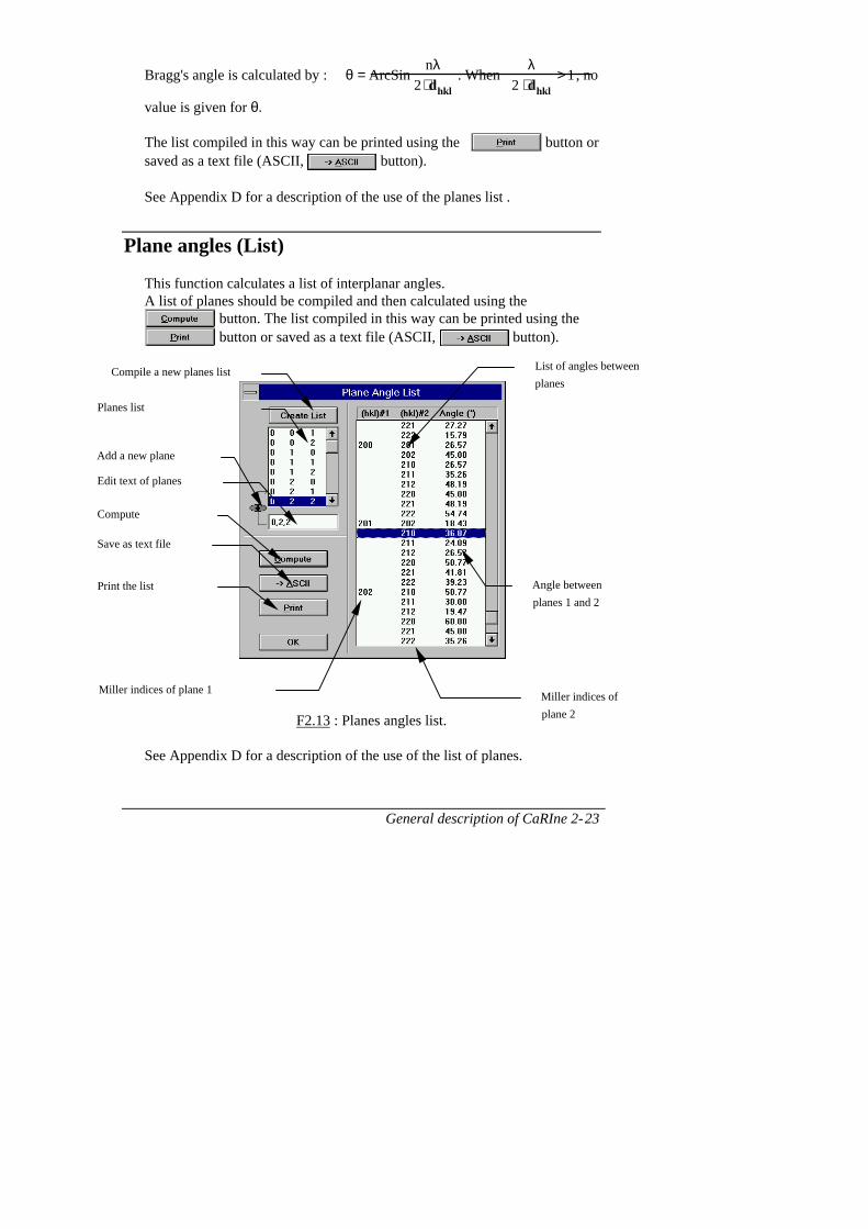
Plane angles (List)
This function calculates a list of interplanar angles.A list of planes should be compiled and then calculated using the
button. The list compiled in this way can be printed using the button or saved as a text file (ASCII, button).
F2.13 : Planes angles list.
See Appendix D for a description of the use of the list of planes.
List of angles between
planes
Angle between
planes 1 and 2
Miller indices of
plane 2
Miller indices of plane 1
Compile a new planes list
Planes list
Save as text file
Add a new plane
Edit text of planes
Compute
Print the list

General description of CaRIne 2-24
Identification of planes
CaRIne allows the planes (hkl) to be identified from an approximateknowledge of their inter planar distance and the angle which is formedbetween them.The values should be entered in the edit text d1 and d2 (in Å) and α (in
degrees) and computed using the button. CaRIne gives anarranged list of possible solutions (max. : 100) in ascending order of error.For each solution, the corresponding zone axis is calculated and displayed.From the zone axis, a cut of the reciprocal lattice can be calculated (seeChap.8 "Zone Axis" function). The list can be printed using the button or saved as a text file ( button).
Application to the indexation of electronic diffraction patterns
α
r1
r2
transmitted beam
spot 1
spot 2
F2.14 : Indexation of diffractionpatterns.
CaRIne can help with the analysis ofelectronic diffraction patterns.
Using the measure of the distances r1and r2 between two spots and the beam
transmitted, and from the angleα which is formed (see fg F2-14)CaRIne indexes the spots andcalculates the corresponding zone axis.CaRIne also provides an arranged listwhich permits any measurement errorof r1, r2 and α to be dealt with.
CaRIne proposes various possibilities :
• Either, you yourself have calculated d1 and d2 :
� these values can be entered directly into the correspondingedit text (in Å),
� next, enter the value of the angle α (in degrees) and click on.

General description of CaRIne 2-25
• Or, you know the constant of the camera K and you measure r1 and
r2. In which case :
� enter K (in cm.Å), r1 and r2 (in cm) in the appropriate edit
text,� click on placed in front of d 1 and d 2, CaRIne then
calculates these values (in Å),� enter the angle α (in degrees),� click on .
• Alternatively, you know the accelerating voltage of the microscopeand the camera length. Measure r1, r2 and α :
� enter the accelerating voltage V in kV,� click on placed in front of λ, CaRIne then calculates the
length of the corresponding wave (in Å),� enter the length of the camera L (in cm),� click on placed in front of K, CaRIne then calculates this
constant in cm.Å,� enter r1 and r2 in cm,� click on placed in front of d 1 and d 2, so that CaRIne
calculates these values (in Å),� enter the angle α (in degrees),� click on .

General description of CaRIne 2-26
F2.15 : Indexation of electronic diffraction patterns : list of possible solutions.
The list is arranged with error values in ascending order :
(∆%) = 100⋅d1m − d1c
d1c
+d2m − d2c
d2c
+αm − αc
αc
�
�
�
�
�
�
where d1m is the measured value of d1, d1c its calculated value (ditto for d2and α).
Miller indices of
planes 1 and 2
Interpalnar distance of planes 1 and 2 Angle between planes 1 and 2
Sum of errors for
d1, d2 and α
Accelerating
voltage
Wavelength
Camera length
Camera constant
Measured
distances
Interplanar
spacings
Angle measured
Calculate
solutions Print solutions Save solutions as text
file (ASCII)
Zone axis
corresponding to
planes 1 and 2

General description of CaRIne 2-27
Formulas used :
• The wavelength (e-) : λ =h
2⋅ m ⋅ e⋅ V, where h is Planck's
constant, m is the mass of electron, e the charge of the electron andV the accelerating voltage.
• The constant of camera K depends on the microscope and possiblythe scale of the diffraction pattern. If the diffraction pattern is on ascale of l:l, then K= λ.L where L is the length of the camera andλ the wave length.
• Inter-planar distance : d =K
r, where r is the measured value of the
diffraction pattern.
Parameters : Search of plane indices up to 10Maximum individual error accepted on d1, d2 and α : 20%
Zone axis of 2 planes
This function calculates the indices u,vand w of the zone axis which correspondsto the data of two planes (h 1k1l1) et(h2k2l2).
The calculation is carried out by pressingthe button.
The formula which is used is given inChap.8 (Reciprocal Lattices).

General description of CaRIne 2-28
Plane // to 2 directions
This function calculates the indices h, k, lof the plane which includes the twodirections [u1v1w1] and [u2v2w2].
The calculation is carried out by pressingthe button.
The formula which is used is given inChap.8 (Reciprocal Lattices).
Count Atoms
This function allows the number of visible atoms to be counted by type(same chemical symbol and same oxidation state).

General description of CaRIne 2-29
2.8 Menu Specials
The Menu Special regroups the functions which are relative to :
• the study of an atom's environment,• the visualisation of plane/direction of rolling,• the X-Ray diffraction patterns,• the stereographic projection,• the reciprocal lattices,• the orientational relationship between several lattices.
Shells
This function shows the successive shells around an atom chosen with themouse. The atoms which constitute a shell are indicated with a cross. Thenumber of atoms belonging to this shell is given along with the distancefrom the centre atom. Please note that only atoms of crystal are taken intoaccount. The following shell is obtained by selecting the
button. For each shell, CaRIne gives a "solid angle"(S.A.%) which is calculated by :
S.A.% = 100 (πri2) / 4πR2
where ri is the radius of the atoms which constitutes the shell and R theradius of the shell. This number can give an idea of the stability of astructure, for example :
R(Å) number ofneighbours
S.A.%
Cubic Primitive 1 6 37.51.41 12 37.5
FCC or HCP 1 12 75.01.41 6 18.75
T2.16 : Environment of atoms in a cubic primitive, F.C.C. and H.C.P.structure.

General description of CaRIne 2-30
With the help of the mouse, it is possible to select shells by clicking on thecalculated list. In this case, only the atoms belonging to these shells will bedisplayed, the others remaining hidden.
e.g. :
The following drawing shows a FCC lattice (2*2*2 cells). The surroundingof the central atom is being studied. Only the first two shells are selected.
F2.17 : Environment of an atom of the FCC lattice.
The function "Multi-Link " Menu Lattice can be used in order to show thepolyhedron edges. Also, the polyhedron function can be used (see 2-31) afterhaving selected one shell, an having made the hidden atoms disappear(function "Remove all hidden atoms" / Menu Crystal).

General description of CaRIne 2-31
Radial Distribution Function
This command traces the radial distribution function, from a selected atomusing the mouse. The result is presented in the form of a histogram. Once astep ("d" in Å) has been chosen, CaRIne distributes the atoms in successiveshells and counts the atoms present in each shell. In this way, the first bar ofthe histogram gives the number of neighbours placed at a distance between 0and d of the chosen atom. The second bar gives the number of neighboursplaced at a distance between d and 2d etc… As for the "shells" function,only atoms on the screen are accounted for.
F2.18 : Radial distribution function (FCC 3*3*3 cells)
Sphere
This function allows the environment of an atom in a sphere of radius r to bestudied. When an atom is chosen with the mouse, CaRIne requests thesphere's radius (in Angstrom), and then hides all atoms which are notcontained in this sphere. The radius of the sphere can be determined by thefunction "Distance between 2 atoms" of the Menu Calcul.

General description of CaRIne 2-32
Polyhedron
This function searches the coordination polyhedrons of your structures.
The central atom should be chosen with the mouse. CaRIne then identifiesthe successive layers of neighbours (see F2.19). In the example which isgiven here (one cell of diamond), there are four first neighbours (covalentcarbon) at a 1.54 Å distance , three second neighbours at a 2.52 Å distanceetc… With the help of the mouse, select the neighbours which are to betaken into account in order to construct the coordination polyhedron. Forthis example, only the first four neighbors will be preserved, and will formthe summit of the tetrahedron .
F2.19 : Research of coordination polyhedrons in a diamond cell.
The function Special/Environment/Polyhedron search allows to previsualizepolyhedron during its construction. Double-click inside the previsualizationwindow to modify the graphic options. Use the mouse (without Ctrl key) torotate the polyhedron or change the scale.
The dialog box "Poly Search" (F2.19) offers two possibilities. The first("Search all same poly.") enables search, within the whole range of crystal,of the polyhedrons which have the same characteristics as the one you areworking on. For example, if the crystal is made up of one diamond cell andthis option is chosen, the four tetrahedral sites are obtained at once, asshown in the following figure (F2.20).
Selected atom

General description of CaRIne 2-33
The second option ("Hide Atoms") can hide the atoms situated at the summitof the polyhedrons. These atoms can be recalled by using the "Recall Atom"function of the Crystal Menu. The hidden atoms can also be deleteddefinitively by using the "Remove all hidden atoms" function of the CrystalMenu.
F2.20 : Visualisation of the tetrahedral sites of a diamond cell.
Isolate
This function allows a polyhedron chosen with the mouse to be isolated.Only this isolated polyhedron will be displayed on the screen. In order tovisualise the whole crystal the isolated polyhedron should be selected asecond time.For a better visualisation of an isolated polyhedron, it is preferable to placethe centre of rotation on the polyhedron's centre atom (see "Around Atom"function of theView Menu).
Texture
This function provides a graphical representation in perspective of theorientation of a lattice in relation to a direction and a plane (the directionshould belong to the plane). The plane corresponds to the plane #1 and thedirection is the current direction (see Menu (hkl)/[uvw]).

General description of CaRIne 2-34
The intersection of the plane with the structure is calculated on one cellonly. The rolling sheet is visualised as a solid rectangle and the intersectionas a hole in this sheet.
To cancel this function and returnto the original representation,click the button.
e.g. :[1,-2,1]
(2,1,0)
F2.21 : FCC in texture view, direction [1 -2 1], plan (2 1 0).
An easy way to define the rolling plane and the direction is to use thefunction "? hkl with mouse" Menu hkl/uvw.Check the plane #1 is visualised ( hkl planes check box in Graphicsoptions / Menu View). Then use the function "? uvw with mouse" and selecttwo atoms of the plane #1 in order to define the rolling direction. Finally,call the "Texture" function and click on .
XRD (powder)
This function enables the calculation of the X-Ray diffraction diagram of thecurrent cell (see Chap.7).

General description of CaRIne 2-35
Stereographic Projection
This function enables the creation of the stereographic projection of thecurrent lattice (see Chap.6).
Reciprocal Lattice
This function enables the creation of the reciprocal lattice of the currentlattice (see Chap.8).
Relation of Epitaxy Ctrl- I
This function allows the orientation relationship between several lattices tobe given in order to fix their relative orientation and to superimpose theirstereographic projections or their x-ray diffraction diagram. This is donewith the study of relationships in matrix/precipitate or substrate/film inmind (see Chap.5).
Associated Lattices Ctrl- L
This function allows real lattices to be associated in order to set their relativeorientation and to superimpose their stereographic projections or theirdiagram of x-ray diffraction. This is done with the study of relationships inmatrix/precipitate or substrate/film in mind (see Chap.5).

General description of CaRIne 2-36
2.9 Menu Crystal
The functions of this menu allow the visualisation of atoms, links andpolyhedrons to be acted upon. Any modifications carried out on thestructure, using the following functions, only concern the crystal and do notaffect the unit cell. For the atoms of the unit cell to be modified the function"Creation" must be used (see p 2-13 and Chap.3 : Creation of a new unitcell) or the function "Crystal to cell" (see p 2- 13).
Most of the functions which enable punctual modifications of the structureand visualisation of the crystal are accessible by the tool-palette (see MenuWindows). When this is the case, an icon appears in front of the function.
Spread of ... Ctrl- F
This function allows the multiplication of the unit cell for each of the a, band c directions. To construct a crystal, the following steps should be taken :
Define the unit cell (Menu Cell) and save it (Menu Files).
Expand the unit cell (this function) in the three directions.
Modify the crystal (modify links, add or remove atoms, display coordination polyhedrons… Menu Crystal).
Select the view and save the crystal (Menu Files).
The function "Spread of ..." proposes two options. The first one consists inmultiplying the unit cell from the original atom situated at a corner of thiscell onwards. This multiplication is carried out from a whole number of cellsfollowing the directions of the vectors a, b and c. The second option enablesthe crystal to be spread in 3 dimensions, beginning at its centre. Real valuescan then be given to the parameters na, nb et nc (see the following example).

General description of CaRIne 2-37
Attention : Keep in mind that, due to CaRIne's logic, by modifying the spreadof a crystal, previous modifications of the crystal will be lost (unless thefunction "Crystal to cell" has been used, see page 2- 13).
e.g. : Construction in relation to the origin of the unit cell of 3*1*2 FCCcells.
F2.22 : Crystal 3*1*2 FCC cell, built from the origin.
F2.23 : Crystal 3*1*2 FCC cells, built from its centre.

General description of CaRIne 2-38
Hide Atom
Click on an atom to hide it. Please note that all hidden atoms can be recalled(they are not erased but saved in "crystal" file). Click a second time on thesame position to hide an atom which is behind the first one.
Hide all
This function allows all atoms or all the atoms of a particular type (chemicalsymbol and degree of oxidation) to be hidden.
Recall
This function recalls a hidden atom. Simply click on the site of a hiddenatom to recall it. If another atom is behind the one that has been recalled,click on a second time
Recall all
After confirmation, this function recalls either all hidden atoms or all theatoms of a particular type. Therefore, do not hesitate to use the "Hide Atom"function to look in the internal structure of a crystal.
Label
This function enables an atom's label (chemical symbol and level ofoxidation) to be displayed or removed, when the atom in question isdesignated with the mouse (see Chap.4). The labels will only appear if thecheck box Labels of the "Graphics" function is checked.

General description of CaRIne 2-39
Label all
After confirmation, this function allows all the atom's labels to be displayed.The labels will only appear if the check box Labels of the " Graphics"function is checked.
Modify Ctrl- M
By clicking on an atom, it is possible to obtain all its attributes :
• chemical symbol and level of oxidation,• the co-ordinates x,y,z in the frame (a,b,c),• the radius (in Angstrom),• the colour,• hidden or not,• vacancy or full site.
F2.24 : Modifying an atom.
It is then possible to change all this information. This function can be usedto displace an atom (to illustrate relaxations or dislocations, for example) orfor example to perform a substitution (using Mendeleev's table). This is thebasic function to be used to represent point defects. To modify the colour,click on the colour box . All atoms identical to the one selected (samechemical symbol, level of oxidation, colour and radius) can be modified bycrossing off the Apply for all same atoms check box.

General description of CaRIne 2-40
If the atom belongs to the plane n°1 (see hkl/uvw Menu), and you wish tomodify all the atoms of this plane, cross off the Apply for plane #1 checkbox. The stacking of planes can rapidly be displayed by giving a particularcolour to the atoms of any same plane (see example 2, Chap.9).
Add Ctrl- A
This function enables an atom to be added, particularly in an interstitialposition. The following steps should be taken :
it is advisable to display the frame (a,b,c) or (x,y,z) (thishelps to find one's bearing within the lattice),
as adding an atom is relative to a full site, select an atomclose to the interstitial site, with the mouse,
enter the coordinates of the vector included between theselected atom and the new atom you would like to add.
F2.25 : Adding an atom.
Please Note: With this function, it is possible to create all types of structure,including organic molecules.
Access to Mendeleev'stable Chemical symbol, level of
oxidation and colour ofnew atom
Atomic radii of newatom
Coordinates of thetranslation vectorwithin the frame(a,b,c)
Coordinates of selectedatom within the frame(a,b,c)

General description of CaRIne 2-41
Vacancy
This function replaces an atom,designated with the mouse, with avacancy (or a vacancy with anatom). A vacancy is represented bya bicolour square (i.e. black and thecolour of the atom).
Remove
This function allows an atom (and its links) chosen with the mouse, to beremoved. Contrary to the "Hide" function, this is irreversible and the atomis erased from memory.
Remove Hidden
After confirmation, this function allows all hidden atoms (and their links) tobe removed. These atoms are then no longer accounted for by CaRIne. Thisaccelerates computing and reduces the size of the corresponding crystal file.
Modify link
F2.26 : Modification of a link.
This function enables a link between twoatoms to be modified using the mouse. Ifyou wish to apply these modifications to allconnections of the same colour andthickness as those designated cross off :
Apply changes for same links.

General description of CaRIne 2-42
Remove
This function allows the link existing between two atoms, designated withthe mouse, to be removed (irreversible).
Remove all
After confirmation, this function allows all links of a crystal to be removed(irreversible).
Add
This function allows two atoms, designed with the mouse, to be linked. Thecolour and thickness of a new link are defined in the " Preferences"function.
Multi link
This function enables certain atomsseparated by a distance d (±epsilon) to be linked. The choice ofatoms to be linked is madeaccording to their chemical symboland their oxida-tion state.
F2.27 : "Multi Link" Function.

General description of CaRIne 2-43
Example : Visualisation of the lamellar structure of graphite.
After loading of the graphitemotif, an unit cell is obtained.
In order to show the stacking ABof graphite, the lattice should bespread to 3*3*1 cells, and then alllinks should be removed.
Ask for the distance between twoatoms which form the edge of one ofthe hexagons (you should obtain1.42 Å).
Choose " Multi Link ", themeasured distance will appear asthe default distance click on
button. After rotationaround xx', the stacking of theplanes ABAB can be visualised.
A
B
A
1,42 Å

General description of CaRIne 2-44
Preferences
This function allows the colour andthickness of each new link to be chosen.Before creating a new structure ( CellsMenu), it is through this function that thetype of link which will form a frame canbe chosen. By default, the colour will beblack and the thickness will be one.
For the thickness of links, it is preferableto use values comprised between 0 and 10.The value 0 allows a minimum thickness,independent of the scale, to be obtained.
F2.28 : Links prefs.
Modify Polyhedron
This function allows a polyhedron, designated with the mouse, to bemodified. All polyhedrons identical to the one chosen (same colour andnumber of sides) can be modified by using the Apply to all similarpolyhedrons check box.
Possible modifications : colour of the sides, colour of the edges, hidden ornot.
Hide
Click on a polyhedron in order to hide it. Note that all hidden polyhedronscan be recalled (they are not erased from memory but saved in a "crystal"file. Click a second time on the same place to hide a polyhedron behind thefirst.
Recall
This function enables a hidden polyhedron to be recalled. Simply click onthe site of a hidden polyhedron to recall it. If another hidden polyhedron isto be found behind this one, click on a second time.

General description of CaRIne 2-45
Recall all
After confirmation, this function recalls all hidden polyhedrons.
Remove
This function allows a polyhedron, designated with the mouse, to beremoved from memory.
Remove hidden
After confirmation, this function removes all hidden polyhedrons frommemory.
Label
This function allows the label of a polyhedron, designated with the mouse,to be displayed or removed (chemical symbols and oxidation state for atomsof summits and for the polyhedron's centre atom).
Label all
After confirmation, this function allows all the polyhedrons' labels to bedisplayed.

General description of CaRIne 2-46
2.10 Menu View
The functions of this menu allows the scales of the real or reciprocal latticesand the parameters of the crystal rotation to be modified.
Graphics Ctrl- G
This function enables modification of the graphical representation of thecurrent crystal, the stereographic projection, the x-rays diffraction diagramor the reciprocal lattice (see §4.5).
Note : The " Graphics" function opens the appropriate dialogue boxaccording to the type of window in use.
General Scale Ctrl- E
Modifies the size of all objects displayed on the screen by entering a valuefor the general scale. This value is proportional to the size of the objects.The general scale should is between 1 and 2000. This function is applied toall real and reciprocal lattices.
Radii Scale Ctrl- X
This function is applied to all real and reciprocal lattices. The atoms size ofa crystal or reciprocal lattice nodes can be modified independently of theother objects.
This allows compact views (radii scale = 100%) or spread views (radii scale< 100%) to be obtained. The value of this scale parameter must be between 1and 400%.

General description of CaRIne 2-47
Example :
Compact view of Al2O3
Radii Scale=100%
Spread view of Al2O3
Radii Scale=25%
F2.29 : Radii scale.
Zoom ±
These two functions give the same result as the function "General Scale".They are, however, easier to use when adapting the size of a crystal to thesize of a window, especially by using the short keys (keys + and -). "Zoom+" corresponds to a multiplication of the general scale by 1.15 and "Zoom -"by 0.85. Note that it is possible to pass through a crystal (try a few"Zoom+"!).
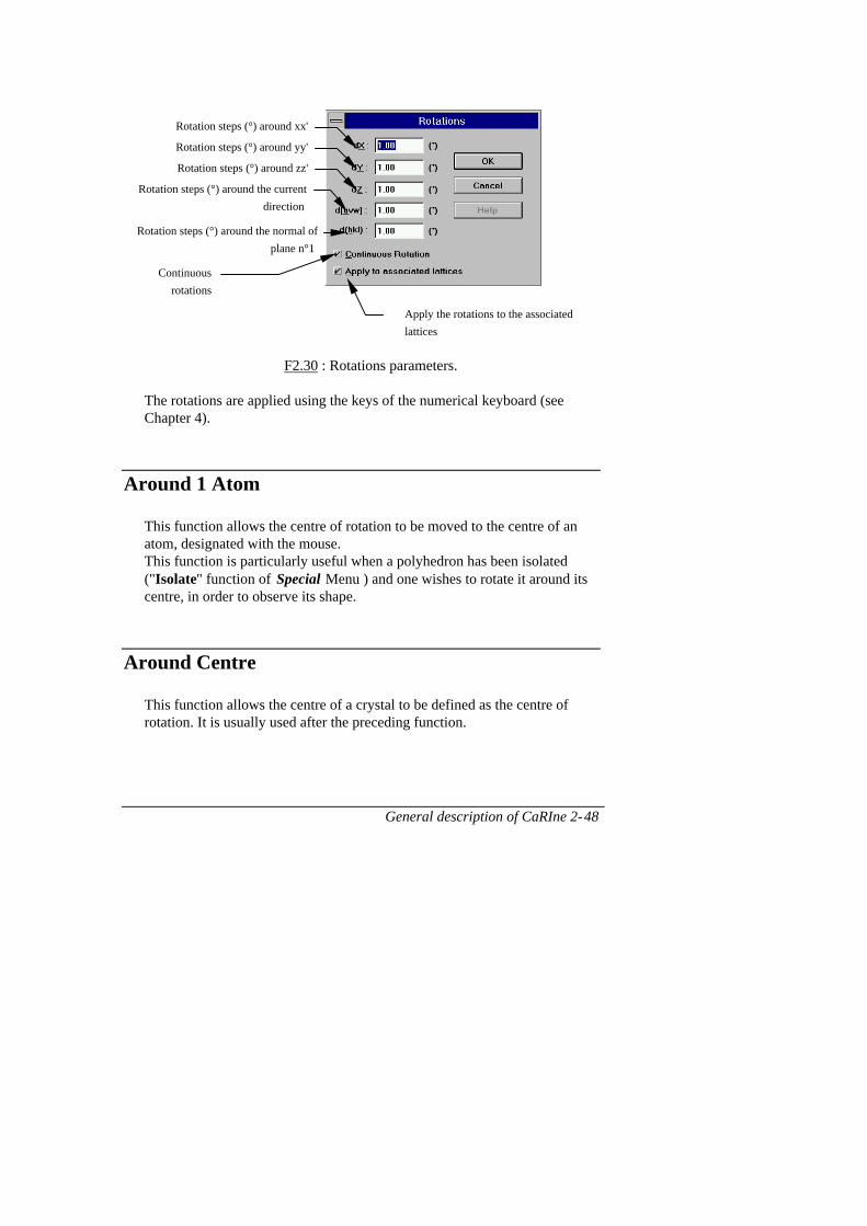
Keyboard Rotations Parameters Ctrl- R
This function enables rotation steps around 5 axes to be set (see Chapter 4.2: Lattice rotations); the continuous rotations function to be activated (Continuous Rotations); and the same rotations to be applied to theassociated lattices ( Apply the rotations to the associated lattices) (seeChapter 5 : Associated Lattices). The value of rotation steps should be givenin degrees.
General description of CaRIne 2-48
F2.30 : Rotations parameters.
The rotations are applied using the keys of the numerical keyboard (seeChapter 4).
Around 1 Atom
This function allows the centre of rotation to be moved to the centre of anatom, designated with the mouse.This function is particularly useful when a polyhedron has been isolated("Isolate" function of Special Menu ) and one wishes to rotate it around itscentre, in order to observe its shape.
Around Centre
This function allows the centre of a crystal to be defined as the centre ofrotation. It is usually used after the preceding function.
Rotation steps (°) around xx'
Rotation steps (°) around yy'
Rotation steps (°) around zz'
Rotation steps (°) around the current
direction
Rotation steps (°) around the normal of
plane n°1
Continuous
rotations
Apply the rotations to the associated
lattices

General description of CaRIne 2-49
2.11 Menu Windows
This menu allows the organisation of CaRIne's windows.
Refresh
Refreshes the active window. This function should be used, for example,after hiding or recalling atoms, or adding links and polyhedrons.
General Tools
This function allows the General Tools palette to be displayed or hidden.This toolbox allows a qwick access to the functions listed below (orderedfrom left to right) :
Files | New
Edit | Copy picture
Edit | Undo/Redo
Files | Print
Files | Print Preview
Cell | Creation/List
Cell | Space groups
Crystal | Spread of...
Special | XRD | Creation
Special | XRD | Preferences
Special | XRD | Save XRD as ASCII file
Special | Stereo. proj. | Creation
Special | Stereo. proj. | Parameters
Special | Reciprocal lattice | Creation
Special | Reciprocal lattice | Spread of...
Special | Reciprocal lattice | Zone axis

General description of CaRIne 2-50
Crystal Tools
This function allows the Crystal Tools palette to be displayed or hidden.This palette allows rapid access to the functions of Menus Crystal (1),HKL/UVW (3), Specials (4) and Calcul (2) :
F2.31 : Crystal tools palette
Stereo.Proj. Tools
This function allows the stereographic projection tool palette to be displayedor hidden. This palette allows rapid access to the functions of the MenuSpecial/Stereo.Proj. :
Remove Atom,Ctrl-click : Remove Hidden (1)Recall Atom,Ctrl-click : Recall All (1)
Modify Atom (1)
Add Link ,Ctrl-click : Link Preferences (1)
Remove Link,Ctrl-click : Remove All (1)Angle Between 2 Directions (2)
Angle Between 2 Planes (2)
? (hkl) with Mouse (3)
RDF (4)
Recall Polyhedron (4)
Hide Polyhedron,Ctrl-click : Hide All (1)
Remove Polyhedron,
Isolate Polyhedron (4)
Add Atom (1)
Hide Atom (1)
Vacancy (1)
Label atom, Ctrl-click : Label All (1)
Modify Link , Ctrl-click : Multi-Link (1)
Distance between 2 Atoms (1)
Angle between Plane and Direction (1)
? [uvw] with Mouse (3)
Shells (4)
Spheres (4)
Recall Polyhedron, Ctrl-click : Recall All (1)
Modify Polyhedron (1)
Label Polyhedron, Ctrl-click : Label all (1)

General description of CaRIne 2-51
F2.32 : Stereographic Projection tools palette.
Rotations Tools
Allows the rotations tools palette to be displayed or hidden (see Chap. 4).
Cascade
This function allows the various windows to be arranged in the form of acascade.
Tile
This function allows the various windows to be arranged in the form of tiles.
...
A window can be activated with the function of the same name.
? direction with mouse,Ctrl-click : Spread of research
Angle with mouse
Trace from 1 pole
Add spot (teta,phi)
Set plane n°1 from spot
Move spot to (teta,phi)
? pole with mouse
Trace from 2 zones
Remove spot
Set [uvw] direction from spot
General description of CaRIne 2-52

Selection of a crystalline structure 3-1
CHAPTER 3Selection of a crystallinestructure
3CaRIne offers four ways of creating crystalline structures.The first way is to use the crystal or cell libraries. It is alsopossible to use the pre-defined Bravais lattices, or to createyour own motifs or unit cells.
3.1 Loading a motif, a unit cell or a crystal from thelibraries
CaRIne is delivered with numerous unit cell and crystal files (seeAppendix B). They can be loaded simply by using the correspondingcommands (see Files Menu). These files can be modified. The librariescan be enlarged with your own creations. All your work can be saved,from the creation of a unit cell (a, b, c, α, β, γ, atoms and theirpositions), to the construction made from the cell (what we call acrystal). It is therefore possible to save as many crystals from the sameunit cell as you wish. The different steps of a complicated constructioncan also be saved. With this method, in case of any problem, it is easy torecall the previous version in order to continue your work.
It is possible to import motifs, cells or crystals in the form of ASCII files(see Files Menu). These structures can then be visualised, modified,printed or inserted into documents. The formats of cells and crystals filesare given in Appendix A. This method can be used to visualise structures

Selection of a crystalline structure 3-2
whose atomic positions have been previously computed, for example, bya molecular dynamics program.
This function also enables cell and lattice files from versions 2.x for MS-DOS and 3.0 for Macintosh of CaRIne, to be imported.
3.2 Use of Bravais' Lattices
It is possible to obtain an example of each of the 14 Bravais latticeswithin just a few seconds. These functions are grouped together in theCells Menu. This is a quick and easy way of illustrating crystallinesystems. It is also a quick way of setting the α, β and γ angles of a newcell. The cell can then be accessed and modified by the function"Creation" of the Cells Menu (see following paragraph).CaRIne automatically sets the cell parameters according to the systemwhich is chosen. Here, since the crystalline system is cubic, a value canonly be given for a (b and c being equal to a, and, α β and γ set at 90°).
Use of Bravais' Lattices
Access toMendeleïev table
Characteristics ofatom
Cellparameters

Selection of a crystalline structure 3-3
Primitive(P)
Body-centred(I)
Base-centred(C)
Face-centred(F)
Cubic
a=b=c
α=β=γ=90°
Triclinic
a≠b≠c
α≠β≠γ
Monoclinic
a≠b≠c
α=β=90° γ qcq
Orthorhombic
a≠b≠c
α=β=γ=90°
Trigonal
a=b=c
α=β=γ≠90°
Tetragonal
a=b≠c
α=β=γ=90°
Hexagonal
a=b≠c
α=β=90°γ=120°
When these functions are used, CaRIne places an atom at each node. Ifone doesn't want an atom at (0,0,0), the "Space Groups" function shouldbe used (see §3.4).

Selection of a crystalline structure 3-4
Note : Please note that once a Bravais lattice has been called, CaRIneloses all memory of the lattice which has been selected. If an atom is thenadded by the function "Creation" (see §3.3), it will not be duplicated onthe equivalent sites of the lattice. If one wishes to obtain this effect, thespace groups must also be used (see §3.4). For example, to create NaCl
from an atom of Na+ at (1/2,0,0) and an atom of Cl- at (0,0,0), the groupFm3 m should be used and not the cubic face-centred function.
3.3 Construction of a new unit cell
It is possible to access cell parameters as well as the list of atoms of themotif at any time, by using the function "Creation" of the Cells Menu. Aquick way of pre-defining cell parameters according to the system is touse the Bravais lattices functions before calling the function "Creation".
To create a new unit cell, the position of each atom must be known.Mendeleev's table can be used to give their characteristics separately(chemical symbol, level of oxidation, radius, colour and occupancy). Thecell can comprise several thousand atoms.
The dialogue box of the unit cell is comprised of 6 edit texts for the cellparameters (a, b, c, α, β, γ), a list of atomic positions, 7 edit texts forentering positions (chemical symbol, level of oxidation, x, y, z, r,occupation factor). One button allows an atom's colour to be modifiedand 4 buttons enable an atomic position to be added, modified orremoved.
The occupation factors enables a percentage of vacancies to be given, thisshould be between 0 and 1 and is used to calculate X-ray diffractiondiagrams.
The atomic positions are reduced coordinates (between 0 and 1) and canbe entered in the form of fractions. The use of fractions is useful in orderto benefit from CaRIne's precision : 1/100 000.
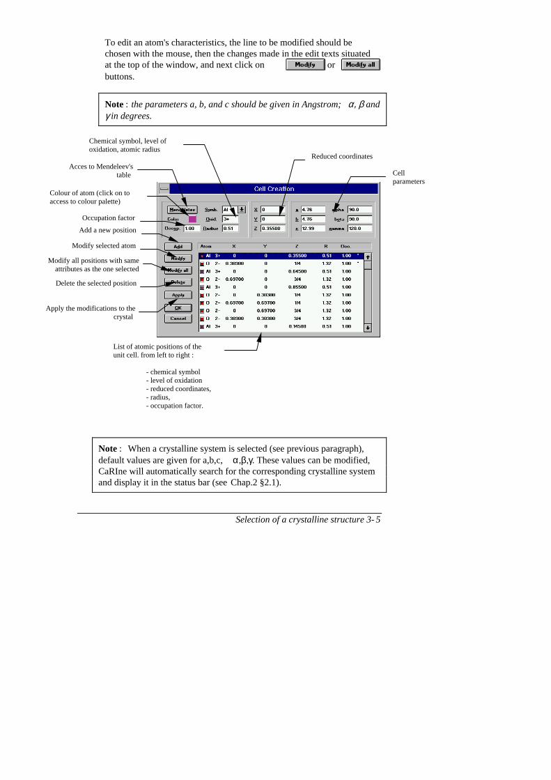
Selection of a crystalline structure 3-5
To edit an atom's characteristics, the line to be modified should bechosen with the mouse, then the changes made in the edit texts situatedat the top of the window, and next click on or buttons.
Note : the parameters a, b, and c should be given in Angstrom; α, β andγ in degrees.
Note : When a crystalline system is selected (see previous paragraph),default values are given for a,b,c,α,β,γ. These values can be modified,CaRIne will automatically search for the corresponding crystalline systemand display it in the status bar (see Chap.2 §2.1).
Reduced coordinates
Cellparameters
Chemical symbol, level ofoxidation, atomic radius
Acces to Mendeleev'stable
Colour of atom (click on toaccess to colour palette)
Occupation factor
Add a new position
Modify selected atom
Modify all positions with sameattributes as the one selected
Delete the selected position
Apply the modifications to thecrystal
List of atomic positions of theunit cell. from left to right :
- chemical symbol- level of oxidation- reduced coordinates,- radius,- occupation factor.

Selection of a crystalline structure 3-6
Description of the different buttons :
• : Add a new position to the unit cell.
• : Modify the selected position (Attention : It is notsufficient to modify the values in the edit texts, this must beconfirmed by using or buttons).
• : Modify all the positions with the same attributes asthe one which has been selected. i.e. modify a position if it hasthe same chemical symbol, level of oxidation, radius and colouras the position selected.
• : Delete the selected position.
• : Apply the modifications to the crystal withoutquitting the dialogue box. The modifications are also applied tothe reciprocal lattice, the stereographic projection and to the x-ray diffraction diagram; if these exist. This function will allowyou to see the consequences of the modifications you areapplying, step by step.
• : Cancel all modifications made to the unit cell sincethe "Creation" dialogue box was opened.
The Creation/list dialog box can be moved or resized with the mouse.All these parameters are saved in the registry.
Header-controls have been added inside this dialog box for the display ofthe atom/position list.
The Rotations tool palette can be used when the Creation/List dialog boxopened (see Chap 4.2.5). This is useful when building a new cell andusing the Apply button. If rotation tools are not visible, you can recall itby pressing the Ctrl key of the keyboard and clicking on the Applybutton.
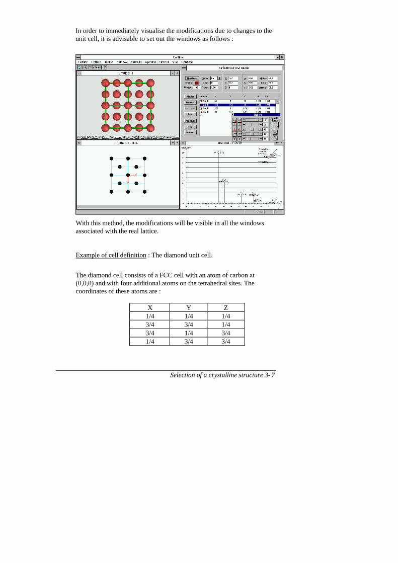
Selection of a crystalline structure 3-7
In order to immediately visualise the modifications due to changes to theunit cell, it is advisable to set out the windows as follows :
With this method, the modifications will be visible in all the windowsassociated with the real lattice.
Example of cell definition : The diamond unit cell.
The diamond cell consists of a FCC cell with an atom of carbon at(0,0,0) and with four additional atoms on the tetrahedral sites. Thecoordinates of these atoms are :
X Y Z1/4 1/4 1/43/4 3/4 1/43/4 1/4 3/41/4 3/4 3/4

Selection of a crystalline structure 3-8
To create the diamond unit cell, simply follow this sequence :
� "New" from the Files Menu, a new window appears,� "Cubic - Face-Centred" from theCells Menu, enter 3.567 Å for a,
choose the carbon atom from the Mendeleev's table,� "Creation" from the Cells Menu, add the four atoms on tetrahedral
sites, when this is done, you should obtain the following :
Remark : using the "Space groups" function one can also define thediamond lattice from the space group 227 (Fd3 m) with only one atom at1/8,1/8,1/8.
Atoms ontetrahedral sitesAtoms of cubic-face
centered

Selection of a crystalline structure 3-9
3.4 Space Groups, construction of a new motif
The " Space Groups " function of the Cells Menu enables theconstruction of a unit cell from a motif and a space group.
The space groups are classified according to the seven crystallinesystems, in order of the group number in Schoenflies 'notation. For eachgroup Hermann-Mauguin's notation is also given.
Once the space group has been selected, a dialogue box is opened inorder to enter non-equivalent positions (i.e. the motif). This box alsoenables cell parameters (a, b, c, α, β, γ) to be attributed to the structure.As with Bravais lattices the cell parameters are set according to thesystem which is chosen.
The 7 crystalline systems
Group number
Allows the search of agroup by its number
List of groups whichcorrespond to theselected system
Group number
Schoenflies' notations
Hermann-Mauguin'snotation

Selection of a crystalline structure 3-10
For the space groups 146, 148, 155,160, 161, 166 , 167 and for all thespace groups of trigonal system, thechoice of whether to use hexagonalor rhomboedral descriptions is leftto the user.
The use of the dialogue box which allows the motif to be entered isdescribed in the previous paragraph.
The choice of space group, the cell parameters and the motif define theunit cell. It is then possible to visualise the resulting positions of all thecell's atoms by using the function "Creation" of the Cell Menu (the non-equivalent positions are marked with an asterix, see § 3.3).
CaRIne conserves in memory the number of the space group and the listof non-equivalent positions. In this way, if a group and a motif havepreviously been defined, it is possible to re-edit them by recalling the"Space Groups" function (attention : this is only possible if the unit cell
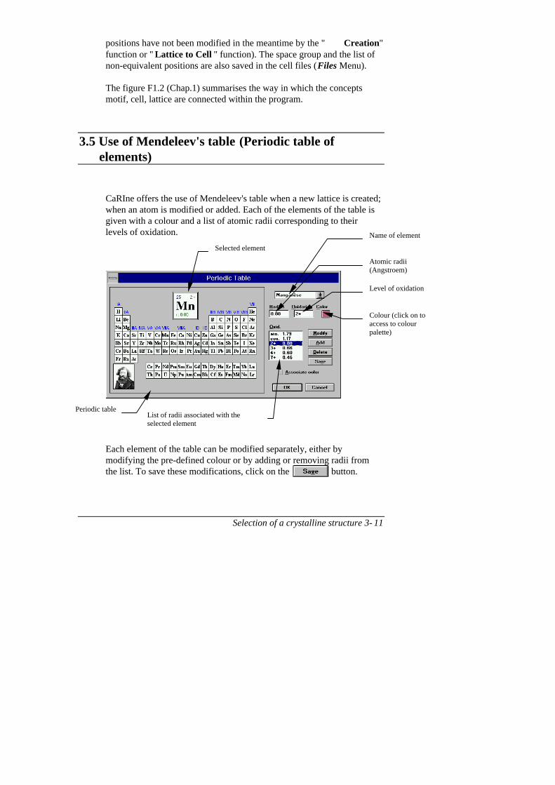
Selection of a crystalline structure 3-11
positions have not been modified in the meantime by the "Creation"function or "Lattice to Cell " function). The space group and the list ofnon-equivalent positions are also saved in the cell files (Files Menu).
The figure F1.2 (Chap.1) summarises the way in which the conceptsmotif, cell, lattice are connected within the program.
3.5 Use of Mendeleev's table (Periodic table ofelements)
CaRIne offers the use of Mendeleev's table when a new lattice is created;when an atom is modified or added. Each of the elements of the table isgiven with a colour and a list of atomic radii corresponding to theirlevels of oxidation.
Each element of the table can be modified separately, either bymodifying the pre-defined colour or by adding or removing radii fromthe list. To save these modifications, click on the button.
Selected element
Name of element
Atomic radii(Angstroem)
Level of oxidation
Colour (click on toaccess to colourpalette)
Periodic tableList of radii associated with theselected element

Selection of a crystalline structure 3-12
An element is chosen by clicking on the corresponding box; the radiusand level of oxidation are chosen by clicking on the list of radii or byentering directly the values into the edit texts Radius and Oxidation.
Note : The valence of a covalent atom is specified by the symbol Coinstead of the level of oxidation state.
The selected element is displayed at the top of the table with thefollowing characteristics : chemical symbol, atomic number, radius andoxidation state.
Atomic number
Oxidation state
Chemical symbol
Atomic radius (Å)
Note : If at least one element of the table has been modified, CaRIneallows the modifications made to be saved.An error message appears if the Mendeleev's table is not in the samefolder as CaRIne (see Installation Procedure Chap.0).

Visualisation Functions 4-1
CHAPTER 4Visualisation functions 4
The visualisation functions are composed of rotations, projections, scalesand the selection of different objects to be displayed.
4.1 The different reference frames of CaRIne
CaRIne works with three different reference frames in 3-D :
• A reference frame linked to the screen, Re
• An orthonormal reference frame which rotates in Re,Rr or(x,y,z)
• A reference frame linked to the unit cell, Rm or (a,b,c).
YY'
XX'ZZ'
Screen
The reference frame linked to the screen(Re) is fixed. It is used as a reference forrotations from the keyboard. The ZZ' axisis perpendicular to the screen, the YY'axis is vertical and the XX' axis ishorizontal.

Visualisation Functions 4-2
a
b
c
x
y
z
αβ
γ
The reference frame (Rm) is defined asfixed within the reference frame (Rr) bythe cell parameters (a, b, c, α, β, γ). (Rm)is formed of the triplet cell vectors (a,b,c).
4.2 Rotations
CaRIne allows a real lattice, a reciprocal lattice or a stereographicprojection to be orientated in five different ways.
Note : The centre of rotation is defined by the functions " Around 1Atom" and " Around Centre " of the View Menu. The first of thesefunctions enables the rotation of a crystal around an atom which hasbeen selected with the mouse. The second redefines the centre of thecrystal as being the centre of rotation.
4.2.1 Using Miller indices
The first is based on the Miller indices. A lattice can be projected eitherfollowing a direction or perpendicularly to a plane. These projectionslead to the direction [uvw] or the normal to (hkl) plane on the ZZ' axis ofthe screen reference frame (Re) (see hkl/uvw Menu).
4.2.2 Using the keyboard
The second way is to orientate, from the keyboard, the reference frame(Rr), and thus the lattice, the stereographic projection and the reciprocallattice. These rotations are carried out within the screen reference frame(Re) around five axes : three of which are the XX', YY', ZZ' of (Re); thefourth, the axis defined by the direction [uvw] (see hkl/uvw Menu) which

Visualisation Functions 4-3
passes through the centre of the lattice; and the fifth, the axis defined bythe normal to plane #1, which passes through the centre of the lattice.The [uvw] direction and the (hkl) plane #1 can be defined using themouse (see hkl/uvw Menu).
The keys to use are :
• <1> and <7> to rotate around the XX' axis,• <2> and <8> to rotate around the YY' axis,• <3> and <9> to rotate around the ZZ' axis,• <4> and <6> to rotate around the axis defined by the [uvw] direction,• </> and <*> to rotate around the axis defined by the normal to plane n°1.
Space bar
Stop rotations
YY' -
XX' -
ZZ' -
[uvw] -
[uvw] +
ZZ' +YY' +
XX' +
Zoom -
Zoom +
Rotations around : (+ positive, - negative)
/ *
(hkl) - (hkl) +
If continuous rotation is required, the box Continuous Rotations("Rotations" function / Menu View) should be crossed off. In this case eachtime one of these keys is pressed, the speed of the rotation is increased ordecreased by the value of the rotation step of the corresponding axis. To stopthe rotations, press the <Space Bar> key. The angles between the x,y,z axesof Rr and the normal to the screen are indicated in the status bar (see Chap.2 -§2.1). These values are given after the symbols : x^n=..., y^n=..., z^n=....
4.2.3 Using the mouse
It is also possible to rotate the crystal or modify the scales using the mouse.Try to move the mouse and press simultaneously the Ctrl key of your key-board and the left button, then with the right button and finally with bothbuttons. Those combinations permit to turn around the 3 axis and allow tozoom.
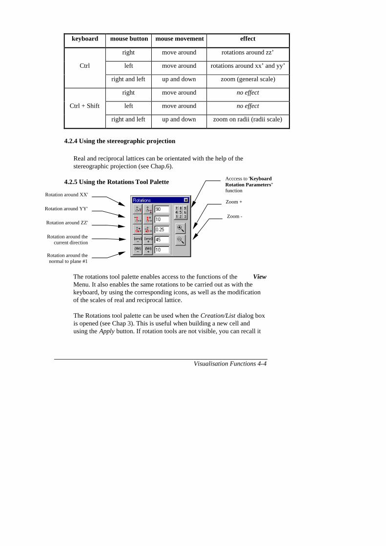
Visualisation Functions 4-4
keyboard mouse button mouse movement effect
right move around rotations around zz’
Ctrl left move around rotations around xx’ and yy’
right and left up and down zoom (general scale)
right move around no effect
Ctrl + Shift left move around no effect
right and left up and down zoom on radii (radii scale)
4.2.4 Using the stereographic projection
Real and reciprocal lattices can be orientated with the help of thestereographic projection (see Chap.6).
4.2.5 Using the Rotations Tool Palette
The rotations tool palette enables access to the functions of the ViewMenu. It also enables the same rotations to be carried out as with thekeyboard, by using the corresponding icons, as well as the modificationof the scales of real and reciprocal lattice.
The Rotations tool palette can be used when the Creation/List dialog boxis opened (see Chap 3). This is useful when building a new cell andusing the Apply button. If rotation tools are not visible, you can recall it
Acccess to "KeyboardRotation Parameters"function
Zoom +
Zoom -
Rotation around XX'
Rotation around YY'
Rotation around ZZ'
Rotation around thecurrent direction
Rotation around thenormal to plane #1

Visualisation Functions 4-5
by pressing the Ctrl key of the keyboard and clicking on the Applybutton.
4.3 Scales
Real and reciprocal lattices have their own scales. These scales can bemodified by pressing the <+> and <-> keys of your keyboard or using themouse (see 4.2.3) :
• <+>: Zoom + (∗ 1.15),• <-> : Zoom - (/ 1.15),
or, using the functions "Zoom ±" and "General Scale" of theView Menu.
4.4 Planes translations
When the visualisation of a particular plane is asked for, CaRIne selectsthe plane of the (hkl) family which is closest to the lattice origin. Theorigin is that of the reference frame (Rm) and can therefore be visualisedby displaying the reference frame (Rm). If the lattice does not haveenough atoms, it is possible that none of the atoms displayed belong tothis particular plane. It is then necessary either to enlarge the lattice (seeCrystal Menu) or to translate the plane. The latter operation correspondsto the function : "Translation ± of a plane" (see hkl/uvw Menu) .
4.5 The "Graphics" command

Visualisation Functions 4-6
The " Graphics" command ( View Menu) allows the graphicalrepresentation of the current crystal, the stereographic projection, the x-ray diffraction pattern or the reciprocal lattice to be modified."Graphics" opens the appropriate dialogue box in accordance with theactivated window :
• In the case of crystal windows, can be displayed separately :
• Atoms : The atoms (which don't belong to selected (hkl) planes).
• Polys : The coordination polyhedrons.
• Frame : The frame and links between atoms.
• Perspective : The perspective effect (cancel it to get a plane projection)
• Colour : The colour of the atoms. When off, the atoms appeartransparent.
• abc, xyz frame : The (a,b,c) and (x,y,z) reference frames (see §4.1).
• (hkl) planes : The atoms which belong to the selected (hkl) plane(s)(see hkl/uvw Menu).
• [uvw] direction : The [uvw] direction is displayed with a red arrow(see hkl/uvw Menu).
• Labels : Display of chemical symbol on atom, with the degree ofoxidation.

Visualisation Functions 4-7
• Background colour: Allows to change the background colour of theactive window.
• Shading Effect: The shading effect is optimal with a thousands colourdisplay.
• Zone Size : The value of each colour zone is given in pixels. Theshading effect is better with a smaller value of the zone size, but theresulting image is larger and the computing time is larger.
• Dephtshading : The intensity of the colours vary as a function of thedistance between the object and the user. The maximum intensity changeis given in the Variation box.

Visualisation Functions 4-8
With shading With atoms and frame
With frame only
With polyhedrons andshading
With polys, frame and shadingWith polys and atoms
a
b
c
x
y
z
With frames and referenceframes (xyz ; abc)
Cl1-
Cl1-
With shading Without shading
Atoms with label
With frame and hkl plane

Visualisation Functions 4-9
• When working in a Stereographic Projection window, can bedisplayed separately :
• Plane traces : The projections of the plane's traces.
• Directions : The projection spots of the directions.
• Poles : The projection spots corresponding to the poles.
• Asso. Lattices : The projections belonging to the associatedlattices.
• Pole indices : The pole indices.
• Direction indices : The direction indices.
• Axes : The projection axes.
• Spot Radii : in pixels.
• Drawing precision : Each trace is composed of this number ofsegments.
• Font size.
• 4 Indices : Cross off this box to get a four indexes output(hexagonal system).

Visualisation Functions 4-10
With poles, directions and traces With axes and poles
• When working in a reciprocal lattice window, can be displayedseparately :
• Frame : The frame of the reciprocal lattice.
• a*b*c* : The reference frame.
• Nodes : The nodes corresponding to theplanes.
• Plane indices.
• Perspective : The perspective effect.
• Font size : The size of the characters.

Visualisation Functions 4-11
(111)
(101)
( 011)(110)
(111)
(001)
(111)
(100)
(010) (111)
(011)
(101)
(110)
(110)
(101)
(011)
(111) (010)
( 100)
(111)
(001)
( 111)
(110) (011)
(101)
(111)
With nodes, indices andframe
With nodes and frame
2,0,-2
2,-1,-1
2,-2,0
1,1,-2
1,0,-1
1,-1,0
1,-2,1
0,2,-2
0,1,-1
0,-1,1
0,-2,2
-1,2,-1
-1,1,0
-1,0,1
-1,-1,2
-2,2,0
-2,1,1
-2,0,2
With nodes and indices
• Finally, in the case of a XRD window, can be displayed separately :
• Associated Lattices : Superposition of the associated lattice XRDdiagrams.
• Plane indices : The planes indices.• Angle and Intensity : The diffraction angle with the relative
intensity.• Bragg Figure : The Bragg's geometry drawing.• Legend : The list of crystals which the XRD diagrams are calculated.• Grid .

Visualisation Functions 4-12
• 2θθθθ1, 2θθθθ2 : These two values give the angle window in which theXRD diagrams are displayed.
• % mini : Minimun intensity for the peaks to be indexed.
Also, the XRD diagrams can be displayed with different options (see Chap 7) :
1) as a list of peaks2) as an intensity versus angle function (squared Cauchy function
with one parameter : the integral peak width β ).3) both 1/ and 2/
With indices, angles and relative intensities With grid and Bragg's figure

Visualisation Functions 4-13
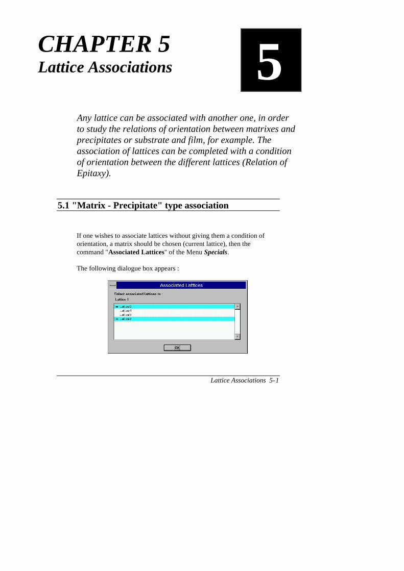
Lattice Associations 5-1
CHAPTER 5Lattice Associations 5
Any lattice can be associated with another one, in orderto study the relations of orientation between matrixes andprecipitates or substrate and film, for example. Theassociation of lattices can be completed with a conditionof orientation between the different lattices (Relation ofEpitaxy).
5.1 "Matrix - Precipitate" type association
If one wishes to associate lattices without giving them a condition oforientation, a matrix should be chosen (current lattice), then thecommand "Associated Lattices" of the Menu Specials.
The following dialogue box appears :

Lattice Associations 5-2
The precipitates should then be chosen from the list of lattices which areopened.
To select or unselect a lattice click on its name. Here the precipitates areLattice 2 and Lattice 5; the matrix being Lattice 1.
If one wishes the precipitates to keep their orientation in relation to thematrix (during rotations and projections), cross off the box Apply therotations to the associated Lattices of the matrix (function "Rotations"Menu View).
Warning : The rotation of a precipitate does not bring about that of thematrix.
In front of each lattice there is a symbol showing the type of association :
� : Matrix-Precipitate association (Matrix � Precipitate )⇐⇐⇐⇐ : Matrix-Precipitate association (Precipitate ⇐⇐⇐⇐ Matrix)⇔⇔⇔⇔ : Crossed Matrix-Precipitate association.
The number of precipitates is unlimited, and it is possible to worksimultaneously with several groups of associated lattices.
Crossed Association
F5.1 : Crossed association.
CaRIne allows crossed associations to be made between several lattices
L2 is the "Matrix" of L1
L1 is the "Matrix" of L2

Lattice Associations 5-3
(see fig F5.1). In this way, a lattice L1 can be the "matrix" of a lattice L2and this same lattice L2 can be the "matrix" of L1. In order to keep theorientation of L1 in relation to L2, while projecting or rotating each of
the two lattices L1 and L2 indiscriminately, cross off the Apply therotations to the associated Lattices box for each of the lattices L1 andL2.
Stereographic Projection, XRD and "Matrix-Precipitate" typeassociation
• The stereographic projection (S.P.) of a matrix M with n precipitatesis the superposition of the stereographic projections of the matrix Mand these of its precipitates P1..n. If the precipitates P1..n are alsothe matrixes M1..n of other precipitates P'1..n, then the S.P. willalso be the superposition of the stereographic projections of theprecipitates P'1..n etc... (see fig. F5.2).
F5.2 : Superposition of stereographic projections
Lattice 2 is precipitate of Lattice 1Lattice 3 is precipitate of Lattice 2

Lattice Associations 5-4
As fig. F5.2 illustrates :
• the stereographic projection of lattice 1 is the superposition ofthe stereographic projections of the lattices 1,2 and 3;
• that of lattice 2 is the superposition of the stereographicprojections of the lattices 2 and 3;
• that of lattice 3 is the stereographic projection of the lattice 3only.
Note : When several stereographic projections are superimposed, theprojection parameters of each lattice must be set separately, byactivating the lattice's windows one by one , then by using the function"Parameters" Menu Special/Stereo.Proj. (see Chap.6 §6.2).
• The X-Ray diffraction pattern of a matrix M of n precipitates is thesuperposition of the X-Ray diffraction patterns of the matrix M andthose of its precipitates P1..n.
In the case of the associative schema of figure F5.2 :
• XRD diagram of the lattice 1 is the superimposition of theXRD diagrams of lattices 1 and 2;
• that of the lattice 2 is the superimposition of the XRDdiagrams of lattices 2 and 3;
• that of the lattice 3 is the XRD diagram of lattice 3 only.
When several x-ray diagrams are superimposed, it is possible to givea proportion to each phase (see Chap. 7).
5.2 Association with "Relation of Epitaxy"
When you wish to associate lattices by giving them conditions oforientation, ask for the command "Relations of Epitaxy " of the MenuSpecials. the following dialogue box will appear :

Lattice Associations 5-5
The lattices to be associated with the current lattice should be chosenfrom the list of the opened lattices.To select or unselect a lattice, click on its name. In order for it to beassociated with the current lattice, cross off the check box which is to theleft of the name (click on a second time to associate or disassociate). Tomodify the plane and direction of epitaxy of the selected lattice, press
.In the example of figure F5.3, the associated lattices are :Lattice 1,Lattice 3 and Lattice 5.
CaRIne automatically associates the lattices of the relation of epitaxy bya relation of crossed matrix-precipitate type. Furthermore, to keep theconditions of orientation due to the relation of epitaxy, CaRIneautomatically crosses off the check box Apply the rotations to theassociated Lattices of each of the lattices of this relation.
The number of lattices associated by a relation epitaxy is unlimited.
Warning : Condition of parallelism : A relation of epitaxy betweenseveral lattices should be given in such a way that all planes are parallelto each other and all directions parallel to one another. However, it ispossible to orient a group of lattices by several relations of epitaxy and tokeep these conditions of orientation (see § 5.3 Orienting a group oflattices by giving several relations of epitaxy).
Plane and directionof the current lattice
Current lattice Plane and direction of the selected lattice(see bellow) Modify the direction
and plane of theselected lattice
Currentdirections
Current n°1 planesList of opened lattices

Lattice Associations 5-6
When the modifications are validated by the button , CaRIneputs the lattices associated in position of epitaxy if and only if :
• all the planes are different from the plane (000),• all the directions are different from the direction [000],• for all the associated lattices, the direction is comprised
within the plane.
Stereographic Projection, XRD and "Relation of epitaxy" typeassociation
The stereographic projection (or the diagram of x-ray diffraction) of alattice which has relations of epitaxy with other lattices is thesuperimposition of the stereographic projections (or the x-ray diffractionpatterns) of this lattice and those of its associated lattices.
5.3 Orientating a group of lattices by giving severalrelations of epitaxy
By using several times the function "Relation of Epitaxy ", a group oflattices can be orientated by several relations of epitaxy which do notcomply with the condition of parallelism of the previous paragraph.
Example : To orientate 3 cubic lattices by the 2 following relations ofepitaxy :
Relation 1 Relation 2Cubic 1 Cubic 2 Cubic 1 Cubic 3(111) // (110) (100) // (102)
[-1-12] // [1-10] [0-10] // [2-2-1]
Once these 3 cubic lattices have been created,
Example :
Lattice 1 Lattice 3 Lattice 5h1k1l1 // h3k3l3 // h5k5l5u1v1w1 // u3v3w3 // u5v5w5

Lattice Associations 5-7
� select the cubic 1 window,� ask for the function "Relation of Epitaxy",� enter the plane (111) and the direction [-1-12] for cubic 1,� select cubic 2 from the list of opened lattices, then enter the plane
(110) and the direction [1-10], press ,� press .
The cubic lattices 1 and 2 are in position of epitaxy and are linked by anassociation of the type "crossed matrix-precipitate".
� select the cubic 3 window,� ask for the function "Relation of Epitaxy",� enter the plane (102) and the direction [2-2-1] for cubic 3,� select cubic 1 from the list of opened lattices, then enter the plane
(100) and the direction [0-10], press ,� press .
The cubic lattices 1 and 2 are in position of epitaxy and are linked by anassociation of the type "crossed matrix-precipitate". The cubic lattice 2has followed the rotation of the cubic lattice 1.
Finally, the following associative schema is obtained :
(100)
(111)
[0-10][-1-12]
Cubic 1
[1-10]
Cubic 2
(110)
Cubic 3
[2-2-1]
(102) : Epitaxy relation # 1
: Epitaxy relation # 2
: "Crossed Matrix-Precipitate" association
F5.3 : Two relations of epitaxy.

Lattice Associations 5-8
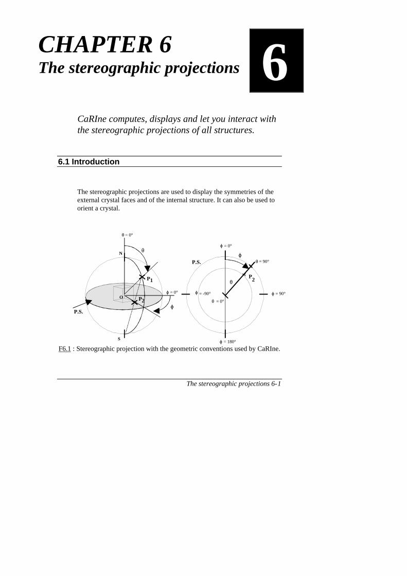
The stereographic projections 6-1
CHAPTER 6The stereographic projections 6
CaRIne computes, displays and let you interact withthe stereographic projections of all structures.
6.1 Introduction
The stereographic projections are used to display the symmetries of theexternal crystal faces and of the internal structure. It can also be used toorient a crystal.
F6.1 : Stereographic projection with the geometric conventions used by CaRIne.
O
N
S
P1
P2ϕ
θ
θ = 0°
ϕ = 0°
P.S.
2θ
θ = 0°
ϕ = 0°
ϕ = 180°
ϕ = 90°ϕ = -90°
θ = 90°P.S.ϕ
P

The stereographic projections 6-2
Consider a sphere surrounding a crystal. From the centre O of the crystaland of the sphere, we can trace the normal to a (hkl) plane. This lineintersects the sphere in P1. This point is called a "pole". This pole can be
located with θ and ϕ angles, as given on F6.1. P1 is projected on theequatorial plane, by drawing a line between P 1 and S. P 2 is theintersection of (P1, S) and the equatorial plane. P2 is the stereographicprojection of the pole P 1. The disk P.S. is called the stereographicprojection.
We can also build the projection of the intersection of an (hkl) plane withthe sphere. To do this, we would choose the (hkl) plane which comprisedthe point o. The intersection of this plane with the sphere is a circle.CaRIne will then project the part of this circle which is located in theNorth hemisphere.
The third kind of objects which can be projected are the directions. Theprinciple is the same as for a pole.
Remark : Only the objects of the North hemisphere are projected onthe stereographic projection.
Notations : For brevity reasons, we will often call "pole (hkl)" the"stereographic projection of an (hkl) pole" (same for tracesand directions).
6.2 Menu Specials/Stereo.Proj.
This menu allows the creation and the use of stereographic projections.
Create
This function creates a new window in order to display the stereographicprojection of the active crystal. The window title recalls the name of thecrystal followed by the "S.P." mention (Stereographic Projection).

The stereographic projections 6-3
The orientation of the stereographic projection corresponds to the crystalorientation, then projections and rotations will have an effect on both thecrystal and its stereographic projection.
The stereographic projection can be copied in the clipboard (WMFformat, see Menu Edit). It is also possible to directly print it or save theimage in a file (see Menu Files).
Use of the protractor :
Each stereographic projectionshas a protractor. It is representedby a cursor which is active whenthe mouse is located inside theS.P. circle. The θ, ϕ coordinatesare given in the information bar(bottom of the window).
θθθθϕϕϕϕ
-180<=ϕ <=0 0<=ϕ<=180
∋θ [0,90]
Parameters
This function is used to build the list of objects to display on thestereographic projection. The objects are the projection spots ofdirections, poles and the projections of plane's traces. With this function,the user can also modify the symbol and colour of the projection spots.
Spots corresponding to directions will be displayed with " empty"symbols, whereas spots corresponding to poles will be "full " symbols. Ifthe current lattice has some associated lattices, the stereographicprojection will be the superposition of the projections of all the lattices.You can choose to use the same directions, poles and traces lists for theassociated lattices, just by clicking in " Use same lists for associatedlattices".

The stereographic projections 6-4
The direction list, pole list, trace of plane list can be loaded and savedfrom/to text files (click on a list box with the right button to select one ofthese functions). Also CaRIne generates the plane form from the entry of3 indices. For example, you can create the (110), (-210), (1-20) list fromthe entry of (110) in the hexagonal system.
A double-click in the stereographic projection (but outside the projectiondisk) will also open the "parameters" dialogue box.
You will find in Appendix D a description concerning the use of thelists.
Create a new list of directions
Create a new list of poles
Create a new list oftraces
List of the tracesList of directions
List of poles
Colour of theprojection
Symbol used forprojection spots
Box used to enter anew direction
Add the direction ofgiven indices
Add the pole of given indicesto list box
Box used to enter a new poleAdd the trace ofplane
Box used to enterthe plane indices
If the lattice has someassociated lattices, usesthe same lists for theassociated lattices

The stereographic projections 6-5
Export to ASCII file
Use the function Special/Stereographic projection/export to an ASCIIfile to export the pole and direction projections polar coordinates (θ φ)into a text file.
Example :
CaRIne Crystallography 3.1
Format : (h,k,l) (or [u,v,w]) teta(°) phi(°)
FCC
Poles(-1,-1,-1) 54.74 -45.00(1,1,0) 90.00 -45.00(1,1,-1) 54.74 135.00(-1,0,-1) 45.00 -90.00(1,0,0) 90.00 -90.00
? [uvw] with mouse
Active this function using the function found in the hkl/uvw Menu orusing the corresponding stereographic projection tool. Then, click insidethe projection circle and CaRIne will answer with the closest [uvw] spot.These u,v,w indexes will be chosen in the range set with the function"Spread of research".
? (hkl) with mouse
Same as previous function, for the (hkl) pole projections.

The stereographic projections 6-6
Spread of search
This function allows the user to modify the range of u,v,w and h,k,lindexes when searching for a direction or pole projection in the vicinityof the mouse location (see functions "? (hkl) with mouse" and "? [uvw]with mouse").
? Angle with mouse
This function gives the angle between poles and/or directionsprojections. Simply select two poles, two directions, or one pole and onedirection with the mouse. CaRIne will answer with a dialogue box whichrecall the indexes of the selected spots and the angle between them.
? Trace from 1 pole
You can add or remove a tracejust by selecting the correspon-ding pole with the mouse. It isthen very easy to see which spotsform a 90° angle with a specificpole.
(111)

The stereographic projections 6-7
? Trace from 2 zones
This function is used to display ornot display the trace of a specific(hkl) plane, from the selection oftwo directions using the mouse.These two directions belong tothe plane.
[110][532]
(111)
first click
second click
Add Spot (teta, phi)
With this function, you will place spots at given (teta,phi) position. Eachspecific spot has a colour, a symbol and a label. If you enter h,k and lvalues as a label (using periods to separate values) CaRIne will display itwith an (hkl) format. Remark that you don't have to give h,k,l indices, allkinds of text being a possible label.
To add a fixed spot, follow this sequence :
� select "Add Spot (teta, phi)" function,� place the mouse to the desired location where you want to
place a spot and click on,

The stereographic projections 6-8
� CaRIne displays a dialogue box and asks to enter a labeland to choose a colour and a symbol. You can change theteta and phi values. Press on .
Remark : If you know the teta and phi values, you can click anyposition on the stereographic projection and just give the teta andphi values in the dialogue box.
This spot will remain immobile. Rotating the crystal or asking forspecific projections will have no effect on its location.
Remove Spot
Just click as closed as possible to a spot to remove it.
Move Spot to (teta, phi)
This function allows the user to orient the stereographic projection andits respective real lattice. The first step is to display the spot that we wantto place on the projection (pole or direction). Then, select the function"Move Spot to (teta, phi) " and click on the pole (or direction) spot.CaRIne answers with the following dialogue box :
(101)
(101)
You can then enter the new values for teta and phi.
Previous location
New location

The stereographic projections 6-9
Set Plane n°1 From Spot
This function allows to define the plane number 1 (see Chap.2 Menuhkl/uvw) from the selection of a pole with the mouse. If you have askedfor the visualisation of planes (function "Graphics" linked to the reallattice), you will see the new plane #1 being actualised.
Set [uvw] From Spot
This function is similar to the previous one. It allows to define thecurrent direction [uvw] (see Chap.2 Menu hkl/uvw) from the selection onthe stereographic projection. This can be used, for example, to define thedirection around which the rotations are done (see Rotation around[uvw]), or to do a projection // [uvw] (see Menu (hkl)/[uvw] ).
Show Spot(teta,phi)
The function Special|Stereo Proj|Display (q,f) allows to display the (q,f)for a specific pole or direction. Simply select this function and click on aspecific spot.
6.3 Orientate the stereographic projection
The sterographic projections can be orientated using different ways :
• Rotations around a [uvw] direction : CaRIne will use the currentdirection of the crystal. This direction can be defined by selecting twoatoms with the mouse (see function " ? [uvw] with mouse " Menuhkl/uvw), by the indices (see function "Choice of [uvw]" Menu hkl/uvw)or by clicking on the stereographic projection (see function "Set [uvw]from spot" Menu Stereo.Proj.).

The stereographic projections 6-10
• Rotations around a (hkl) pole : CaRIne will use the plane #1 of thecrystal (Menu hkl/uvw). This plane can also be defined using thefunction "Set (hkl) from spot".
• Move a pole or a direction spot to a specific position :
� functions "Projection // [uvw] " or " Projection Perp. (hkl) "(Menu hkl/uvw) (place the current direction or plane at the centreof the projection).
� function "Move spot to (teta, phi)" (see §6.2).
� using the mouse :To move a spot on the stereographic projection, press the Ctrl keyof the keyboard and click on a specific spot, and move the mouse.
To move the stereographic projection around a spot (i.e. rotate thecrystal around a direction or a pole), press the Ctrl Key of thekeyboard, then select a spot with a double-click. A symbol appearsto show that this spot is now fixed ( ). You can now move thestereographic projection as explained before. Perform anotherdouble-click on the fixed spot () in order to free it.
This function allows to use the stereographic projection as an easy tool toorientate the crystal and also the reciprocal lattice.
6.4 Menu View
Graphics Ctrl- G
This function opens the dialogue box dedicated to the graphic optionsrelative to the stereographic projection. It is possible to display the poles,directions or plane traces separately or together. This option also allowsyou to modify the font size (see Chap.4).

The X-Ray diffraction patterns for powders 7-1
CHAPTER 7The X-Rays diffraction patternsfor random orientated powders
7CaRIne computes the positions and intensities of theX-Rays diffraction peaks from the knowledge of theunit cell.
7.1 Introduction : Calculation of peak intensities
The calculation of the X-Rays diffraction is done from the unit cell, for arandom orientated powder, and with the Bragg configuration as shownbelow :
o 2
θ
θλ
F7.1 :Bragg's geometric configuration.
The θ angle is called Bragg angle.
The diffraction angle is calculated from the interplanar distance andfrom the incident wave length λ :

The X-Ray diffraction patterns for powders 7-2
λ θ= ⋅��� ��2 hkld
nsin (E7.1)
For each (hkl) plane, the structure factor is computed using equationE7.2 :
Fhkl = fn . focc.e2πi (h.xn +k .yn + l .zn )
n=1
N�(E7.2)
where fn is the atomic scattering factor for x-rays; xn, yn et zn are the
coordinates of the nth atom of the cell; focc is the occupation factor ofthe site (0� focc� 1).
The atomic scattering factors vary as a function of the Bragg angle andthe x-ray wave length.
CaRIne uses the following approximation :
fsinθ
λ
� �
�
= ai . e
− bi .sin θ
λ
�
�
� � �
2
i=1
4�+ c (E7.3)
where ai, bi et c are fitting coefficients. The list of the different ionswhich are differentiated is given in Appendix C.
To compute the peak intensities, CaRIne takes into account the followingfactors :
- the Lorentz factor :
f Lorentz =1
4.sin2 θ.cosθ(E7.4)
- the polarisation factor :
f Polarisation=1
2. 1 + cos2 θ( ) (E7.5)

The X-Ray diffraction patterns for powders 7-3
- the temperature factor (supposed to be constant for all atoms of thecell) :
f Temperature= e
−2.B.sinθ
λ
� �
� �
2
(E7.6)
Remark : the temperature factor is given by the user.
- the multiplicity factor, which depends on the (hkl) plane and on theunit cell.
Finally, the intensities of the peaks are computed as :
I
F e p
V
B
=⋅ +
⋅
��� �� ⋅ ⋅− ��� ��2
2
2
21 22
cos
sin cos
sinθθ θ
θλ
(E7.7)
where V is the unit cell volume.
And these intensities are normalised relatively to the highest peak.
Remark : the absorption factor is not taken into account in thecomputation of the normalised intensities because this factor isindependent of θ :
f Absorption =1
2µ(E7.8)
But this should be remembered when doing powder mixing, and the usershould enter this factor in the proportion coefficient for each phase (seefunction "Create" §7.2).

The X-Ray diffraction patterns for powders 7-4
7.2 Menu Special/XRD (powder)
Create
This function computes the powder-XRD of the current crystal.
A dialogue box appears, in which the different parameters can be set up.Then, you have to choose :
the wavelength of the X-Rays (you can either enter a value orclick on one of the proposed ones), the minimum and maximum Bragg angles, the temperature factor, in the case of existence of associated lattices to the currentcrystal, these lattices appear in the "Mixture" box. Afterselecting one of these using the mouse (simple-click), youcan change its multiplication factor (2.00 in our example).The calculated intensities will be multiplied by this factor,and then, normalised to the most intense peak of all presentphases.
Minimum andmaximum Bragg angles
List of associated lattices
Click on this button tochange the multiplicationfactor of the selectedphase
Wavelength
Temperature factor

The X-Ray diffraction patterns for powders 7-5
A double-click on a phase name in the "mixture" box allows to access tothe graphic parameters (colour and motif of the lines). This is equivalentto the "Preferences" function (see below).
After this set-up, you can click on . CaRIne creates a newwindow in order to display the X-Rays diffraction diagram. The title ofthis window recall the name of the real lattice with the mention "XRD(powder)".
The diagram can be copied (Menu Edit), printed (Menu Files) or savedon disk as a picture (Menu Files).
A double-click inside the XRD window re-opens the parameters dialogbox.
Note :If one wants to change the mixture coefficients without recalculation ofthe XRD pattern, the Mixture function should be used (see page 7-6).
Preferences
This function gives a colour and a motif to the diagram corresponding tothe real lattice active window. Initially, all diagrams are drawn in blackwith solid lines.
Save XRD as ASCII File
This function allows to save the XRD diagram calculated by CaRIne asan ASCII file.
Example :
CaRIne Crystallography 3.0C:\CARINEV3\CEL\CL\NACL.CELMax. value : 429664.312

The X-Ray diffraction patterns for powders 7-6
Number of peaks : 15(hkl) 2teta intensitydhkl fs² P(200) 32.53 100.0 2.750 6305.233(400) 68.14 6.1 1.375 1990.763(600) 114.35 1.2 0.917 571.18 3(420) 77.56 14.3 1.230 1500.0812(220) 46.67 56.4 1.945 3958.816(440) 104.79 2.8 0.972 715.92 6(531) 111.90 0.8 0.930 48.93 24(511) 93.39 0.4 1.058 56.34 12(331) 75.25 0.6 1.262 61.11 12(311) 55.36 1.5 1.658 76.72 12(111) 28.08 8.6 3.175 296.54 4(442) 114.35 4.9 0.917 571.18 12(422) 86.65 9.5 1.123 1156.0412(222) 58.04 15.8 1.588 2733.144(333) 93.39 0.1 1.058 56.34 4
Mixture
This function allows the user to affect a coefficient to every phase fordiffraction pattern of a powder mixture.
Import Exp. File
This function allows the user to import its own experimental data file.This file (ASCII File) should respect the following format :
• first line (header) : XRD Exp. File,• the second line gives the number of values in the file,• then, the file is a succession of lines with two values
separated with "spaces" or "TAB". The first value of eachline is the diffraction angle (°) . The second value is theintensity.

The X-Ray diffraction patterns for powders 7-7
Example :
XRD EXP. File2098.0000 38.508.2500 34.508.5000 36.258.7500 35.259.0000 42.509.2500 43.259.5000 32.50...
Prefs. Exp. File
This function allows to change the colour and motif of the experimentaldiagram (see previous function). Initially, these options are set to blackand solid lines.
Remove Exp. File
This function allows to remove the experimental diagram (see previousfunctions).
Import Ref. File
This function allows the user to import its own reference datafile(ASTM, JCPDS, ...). This file (ASCII file) should respect the followingformat :
• first line (header) : XRD Ref. File,• the second line gives the number of peaks in the file,• then, the file is a succession of lines with 5 values separated
with "spaces" or "TAB". The first value of each line is theinterplanar distance . The second value is the intensity.

The X-Ray diffraction patterns for powders 7-8
These intensities should be normalised in order that thehighest intensity is 100. And the three last values are theindexes of the hkl plane.
Example :
XRD Ref. file606.583 34 1 0 03.800 35 1 1 03.293 100 2 0 02.660 99 2 0 02.489 93 2 1 02.31 9 1 1 12.1939 10 3 0 02.1797 31 2 0 1etc...
Prefs. Ref. File
This function allows to change the colour and motif of the referencediagram (see previous function). Initially, these options are set to blackand solid lines.
Remove Ref. File
This function allows to remove the reference diagram (see previousfunctions).

The X-Ray diffraction patterns for powders 7-9
7.3 Menu View
Graphics Ctrl-G
This function allows the graphic objects to be selected independently : X-Rays diffraction diagrams of associated lattices, plane indices, angle andintensity of each peak, grid, envelopes…
Intensity (%)
2 θ (°)
40 50 60 70 80 90 100 110 118
0
10
20
30
40
50
60
70
80
90
100o
(1.540562 Å)θ ∈ [ 20°,60°]B = 2.0 Ų 2θ
θ
E:\....02\Cry\RX\Nacl.cry
4,0,0 6,0,04,4,2
4,2,0
2,2,0
4,4,05,3,13,1,1
4,2,2
2,2,2
The XRD diagrams can be displayed with different options :
1) as a list of peaks,2) as an intensity versus angle function (squared Cauchy function
with one parameter : the integral peak width β )3) both 1/ and 2/

The X-Ray diffraction patterns for powders 7-10
Option 2 allows the summation of several diagrams when using theassociation of lattices (mixture of powders).
Note :
Squared-Cauchy function : ( )
I(x)Imax
1 k x2 2=
+ ⋅
The integral width is given as : β π=2 k
Then CaRIne computes k as : k =⋅
!"# $%πβ2
2
The FWHM (full width at half maximum intensity) is given by : lk
=−2 2 1
Change XRD scales with the mouse :
Cursors under the Bragg angle axis can be moved with the mouse inorder to perform zooms. A double-click between cursors in the info-bargets back to the original teta range (full scale). Another new functionpermits to display only most intense peaks infos (θ, intensity, indices).To do so, simply move the cursor with the mouse, on the intensity axis.
Move these cursorsto change scale
Double click between cursors to showfull scale. Click between cursors andmove the mouse to translate the view
Move this cursorto display onlymost intense peaksinfos
Translate the view

The Reciprocal Lattices 8-1
CHAPTER 8The Reciprocal Lattices 8
CaRIne build and visualises the reciprocal latticefrom the direct lattice.
8.1 Introduction
The reciprocal lattice is defined from the direct lattice vectors, as :
a* =b^c
V, b* =
c^a
V, c* =
a^b
Vwhere V is the cell volume, V = a . (b^c).
The parallelepiped built on a*,b*,c* is called the unit cell of thereciprocal lattice.
For each plane of the direct lattice corresponds a node of the reciprocallattice. For each planes' family only in the direct lattice corresponds to aninfinity of reciprocal lattice points, aligned on a direction normal to theplanes.
The direct and reciprocal lattices are conjugated and have the same pointsymmetry. But their space groups are generally differents.
In the CaRIne software, the relative orientation of a, b, c and of a*, b*,c* vectors is always respected. Rotating the direct lattice will then inducethe corresponding rotation of the reciprocal lattice. As for the real lattice

The Reciprocal Lattices 8-2
you can use the «intuitive rotations» with the mouse (see §4.2.3).General scale and radii scale can also be modified using this way.
The norms of the a*, b*, c* vectors will also be automatically computedas soon as the vectors a, b, c are modified. Nevertheless, the reciprocallattice scale allows the zoom in/out of each lattice independently (seeChap.4 §4.3).
In the reciprocal lattice, a family of (hkl) planes is represented by a nodeM such as :
dhkl* = OM* =h.a* + k.b* + l.c*
So, a vector dhkl*
of the reciprocal lattice represents the orientation of
the planes' family in the crystal ( dhkl*
⊥ (hkl) ) and the interplanar
distance (dhkl =1
dhkl*
). CaRIne allows to take angles and distances in
the reciprocal lattice, using the mouse.
As for the direct lattice (see Chap.1 §1.4), it is possible to work in twodimensions in the reciprocal lattice :
1/ first, of all one can show (h k 0) nodes by using the "Spread of... "function (see Chap. 8.2). It is then possible to do a projectionperpendicular to the (001) plane.
2/ second, by one can visualise a "cut" of the reciprocal lattice,perpendicularly to a [uvw] zone axis (see Chap. 8.2, function "Zoneaxis"). This function can be very useful for electron diffraction patternanalyses.
Structure factor calculations :
When CaRIne build the reciprocal lattice, the structure factors arecomputed for each (hkl) family, with the atomic scattering factors takenas f = Z (electron number, taking into account the oxidation level). In thecase of no chemical symbol name has been assigned to atoms, the "f"

The Reciprocal Lattices 8-3
factors are set to "1". In this case, the spheres of the real lattice can beconsidered as lattice points.
If the structure factor Fhkl is different from "0", a node for hkl will beshown in the reciprocal lattice.
hklF = nf ⋅n=1
N�2πi(h⋅x n + k ⋅yn + l⋅zn )
e
where xn,yn,zn represent the position of the nth atom in an elementarycell of N atoms.
The origin (0,0,0) of the reciprocal lattice is shown by a cross-centred
circle ( ).
Example :
The face-centred cubic real lattice produces a body-centred cubicreciprocal lattice :
1/ Select "Cubic" and "Face-centred (F) " in the Menu Cell (donot give names to atoms)2/ create the reciprocal lattice, with h,k,l between 0 and 2.
FCC real lattice
�
Reciprocal lattice

The Reciprocal Lattices 8-4
Some geometric relationships :
• The Weiss zone axis law :
If (hkl) belongs to the [uvw] zone, then hkl*
d ⋅ uvwd = 0
• Relations between the direct lattice vectors and the reciprocal latticevectors :
c* . a = 0 c* . b = 0a* . b = 0 a* . c = 0b* . c = 0 b* . a = 0
• The addition rule :
1h + 2h , 1k + 2k , 1l + 2ld * =
1h 1k 1l
*d +
2h 2k 2l
*d
• The zone axis of two planes :
uvwd =1h 1k 1l
*d ∧
2h 2k 2l
*d
i.e. : u = k1l2 - k2l1v = l1h2 - l2k1w = h1k2 - h2k1
• The plane containing two directions :
hkl
*d =
1u 1v 1wd ∧
2u 2v 2wd
i.e. : h = v1w2 - v2w1k = w1u2 - w2v1l = u1v2 - u2v1

The Reciprocal Lattices 8-5
• The interplanar distance :
1
hkld
=hkl
*d
• The normal to a plane :
hkln = hk l
*d
hk ld
• The angle between two normals :
cosθ = h1k1l1*d •
h2 k2l 2*d
h1k1l1*d
h2 k2l 2*d
All these relationships are widely used by the CaRIne software.

The Reciprocal Lattices 8-6
8.2 Menu Specials/Reciprocal Lattice
Using this menu, you will be able to create the reciprocal lattice, tochange its spreading or to make a plane cut by selecting a zone axis.
Creation
This function creates a new window where the reciprocal lattice will bedisplayed. The title of this new window will correspond to the directlattice from which it has been created.
The reciprocal lattice follows the orientation of the real lattice(projections, rotations,…).
It is possible to copy the reciprocal lattice in the clipboard (WMF format,see Menu Edit), to print or save the image on a disk (see Menu Files).
The calculation of the reciprocal lattice takes into account the structurefactors. In case of an extinction, the radius of the corresponding sphere isnull, and the plane indices are not displayed.
Spread Of...
This function allows the spreading of the reciprocal lattice in the 3directions (h, k and l). If you desire to cut the reciprocal lattice by aplane normal to the zone axis (the zone axis indices correspond to thecurrent [uvw] direction), you will simply have to check the check box Using zone axis (see the following function).
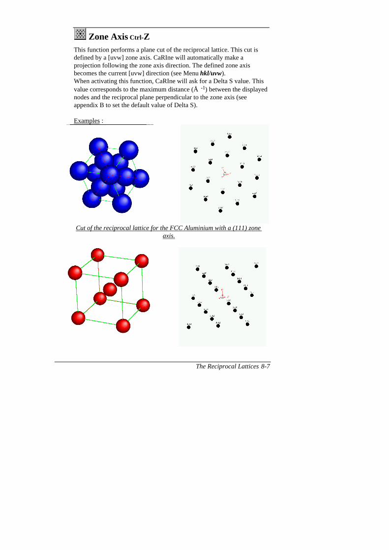
The Reciprocal Lattices 8-7
Zone Axis Ctrl-ZThis function performs a plane cut of the reciprocal lattice. This cut isdefined by a [uvw] zone axis. CaRIne will automatically make aprojection following the zone axis direction. The defined zone axisbecomes the current [uvw] direction (see Menu hkl/uvw).When activating this function, CaRIne will ask for a Delta S value. Thisvalue corresponds to the maximum distance (Å-1) between the displayednodes and the reciprocal plane perpendicular to the zone axis (seeappendix B to set the default value of Delta S).
Examples :
Cut of the reciprocal lattice for the FCC Aluminium with a (111) zoneaxis.

The Reciprocal Lattices 8-8
Cut of the reciprocal lattice for the BCC Iron with a (112) zone axis.
? dhkl with mouse
This function gives the interplanar spacings of (hkl) planes just byselecting the corresponding node of the reciprocal lattice, with themouse. This value is then inversely proportional to the distance betweenthe selected node and the origin of the lattice.
? angle hkl with mouse
This function gives the angle between two planes, by selecting theirnodes on the reciprocal lattice.

The Reciprocal Lattices 8-9
8.3 Menu View
This menu allows the selection of the graphical options.
Graphics Ctrl-G
As for the direct lattice, this function allows to select independently theobjects to be displayed : nodes, indices, reference frame, links. It is alsopossible to activate/deactivate the perspective view.
General Scale Ctrl-E
This function acts on the size of all the reciprocal objects. The value ofthe scale is directly proportional to the object sizes (between 1 and 2000).
Note that this scale is independent from the real lattice scale.Nevertheless, proportions are respected. For example, if we increase thesize of the real lattice by a factor 2, then the size of the reciprocal latticeobjects will be decreased by a factor 2.
Radii Scale Ctrl-X
The size of the reciprocal lattice nodes can be modified independentlyfrom the other objects.

The Reciprocal Lattices 8-10
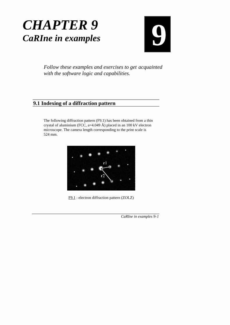
CaRIne in examples 9-1
CHAPTER 9CaRIne in examples 9
Follow these examples and exercises to get acquaintedwith the software logic and capabilities.
9.1 Indexing of a diffraction pattern
The following diffraction pattern (F9.1) has been obtained from a thincrystal of aluminium (FCC, a=4.049 Å) placed in an 100 kV electronmicroscope. The camera length corresponding to the print scale is524 mm.
F9.1 : electron diffraction pattern (ZOLZ)

CaRIne in examples 9-2
Question : Index the diffraction spots and determine the zone axis.
Solution :
1/ Without CaRIne
a/ take distances and angles on the diffraction pattern;b/ determine the extinction conditions in the FCC lattice;c/ make a list of the (hkl) planes with their interplanar spacings;d/ compute the corresponding distances on the film;e/ determine the different possibilities of indexing, check that the
angles are correct, determine the zone axis.
2/ Using CaRInea/ take distances and angles on the diffraction pattern;b/ load the aluminium FCC unit cell from the cell library (Menu
Files, function "Load Cell") or create this cell using the FCCBravais' lattice. Check that a=4.049 Å;
c/ use the " Identification of Planes " function from the MenuCalcul :- enter the accelerating voltage (100kV) and select the
button which will compute the corresponding wavelength(0.0388 Å);
- enter the camera length (52.4 cm) and select the buttonwhich will give the camera constant (K=2.03 cm.Å);
- enter two distances, obtained from the diffraction pattern,with the angle between the two spots (for example,r1=0.85cm and r2=1.6cm and α= 58.5°). Click on tocompute the corresponding interplanar distances (you shouldget d1=2.39Å and d2=1.27Å);
- click on .
As a result of this sequence, CaRIne answers with a list ofpossibilities, ordered according to the increasing error between thecomputed solution and the experimental data. For the presentexample, the {111} - {311} solution with a [221] zone axiscorresponds to a sum of errors (on d1, d2 and α) of 6.1%. Thefollowing solution {111} - {221} with a [110] zone axis,corresponding to a sum of errors of 14.9%.

CaRIne in examples 9-3
Now, we just have to show these 2 solutions in order to choosebetween them. To do so, we need to create the reciprocal space(Menu Special / " Reciprocal lattice "-"Create"). To obtain the"3" indices, use the Menu Special / " Reciprocal lattice " -"Spread of"). Ask for the desired zone axis ([221] and [110
�)
using Menu Special / " Reciprocal lattice" - " Zone axis"). Thefigure F9.2 shows these results.
(131)
(022)
(113)
(333)
(222)
(111)
(111)
(222)
(333)
(113)
(022)
(131)
a*
b* c*
(333)
(331)
(331)(222)
(113) (220) (333)(111) (222)
(002) (111)
(113)(113)
(111) (002)(222) (111)
(333) (220) (113)
(222)(331)
(331)
(333)
a*
b* c*
F9.2 : Plane cuts of the reciprocal lattice computed by CaRInea) left : zone axis [211] b/ right : zone axis [110].
Comparing the F9.2 with F9.1 clearly shows that the correctsolution is [211]. The diffraction pattern is automatically indexed.

CaRIne in examples 9-4
9.2 Standard projections of a cubic crystal
Question : Trace the standard projections (001) and (011) of a cubiccrystal. Show the planes lying in a 100, 001, 110, 111 or 112 zone on astereographic projection.
Solution :
The sequence to follow is given below :
1/ Create a simple cubic lattice : a simple way to do so is to use MenuCell / function "Cubic " - "Simple".
2/ Create a stereographic projection. You can either call the function"Create" from the Menu Specials/Stereo. Proj. , or click on thestereographic projection icon (below the rotation tools).
3/ Ask for the display of all indices between -1 and 1 : click on thestereographic projection window, outside of the circle. You can alsouse the function " Parameters" from the Menu Specials/Stereo.Proj.. In the dialogue box, click on (and later on )and give the indices ranges.
4/ Orient the stereographic projection : this can be done by using theMenu hkl/uvw function "Proj. perp. plane ", after having selectedthe plane #1 in the planes dialogue box (function "Choice of hklplanes" from the Menu hkl/uvw). You will get the following figures:

CaRIne in examples 9-5
(111)
(110)
(110)
(111)
(101)
(100)
(100)
(101)
(111)
(110)
(110)
(111)
(011)(010) (010)(011)(001)
(111)
(110)
(111)
(111)(101)
(100)
(100)
(101)
(111)
(111)(110)
(111)
(011)(010) (011)(011) (001)
F9.3 : Stereographic projection a) left : 001 b) right : 011.
To visualise the planes perpendicular to a specific plane, we can build astereographic projection with all the poles with indices between -3 and+3. Then, we add the trace of the specific plane. The poles lying on thetrace are the solutions (see F9.4).
(101)
(313)
(312)
(311)
(310)
(310)
(311)
(312)
(313)
(323)
(322)
(321)
(320)
(320)
(321)
(322)
(323)
(201)
(302)
(301)
(100)
(100)
(201)
(301)
(302)
(101)
(102)
(103)
(113)
(112)
(203)
(213)
(212)
(211)
(210)
(210)
(211)
(212)
(213)
(223)
(313)
(312)
(311)
(310)
(310)
(311)
(312)
(313)
(323)
(322)
(321)
(320)
(320)
(321)
(322)
(323)
(111)
(221)
(332)
(331)
(110)
(110)
(221)
(331)
(332)
(111)
(112)
(113)
(123)(122)
(121)
(120)
(120)
(121)
(122)
(123)
(133)(132)
(131)
(130)
(130)
(131)
(132)(133)
(001)(013)(012)(011)(032)(031) (021) (010)(010) (031)(032)(021)(011)(023)(012)(013)(023)
(223)
(233)
(232)
(231)
(230)
(230)
(231)
(232)
(233)
(103)
(113)
(112)
(111)
(332)
(331)
(221)
(110)
(110)
(331)
(332)
(221)
(111)
(223)
(233)
(232)
(231)
(230)
(230)
(231)
(232)
(233)(112)
(113)
(123)
(122)
(121)
(120)
(120)
(121)
(122)(123)
(133)(132)
(131)
(130)
(130)
(131)
(132)(133)
(102)
(203)
(213)
(212)
(211)
(210)
(210)
(211)
(212)
(213)
(223)
F9.4 : 001 projections in the cubic system, of the poles with indices between -3and +3, and the traces of planes (100), (001), (110), (111) and (112).

CaRIne in examples 9-6
9.3 ABCABC… sequence in FCC and ABAB…sequence in HCP
Question : Show the sequence of compact planes in the FCC and HCPlattices.
Solutions :
a/ For the FCC structure, we want to show the construction of the lattice as aABC stacking of {111} planes :
1• Open a new window (Menu File / function "New" or Ctrl-N).2• Select a face-centred cubic lattice (Menu Cells / function
"Cubic/Face-Centred (F)") and choose an atomic radius of 1Å witha lattice parameter of a=2.828Å in order to get a compact structure. Itis not an obligation to select a chemical symbol and a level ofoxidation for the element.
3• To work in several cells, expand the lattice using Menu Crystal /function "Spread Of...".
4• Select the (111) as the plane #1 in the plane dialogue box (Menuhkl/uvw / function "Choice of hkl planes").
5• Change the colour of all atoms belonging to a particular (111) plane :use the function "Modify atom" (Menu Crystal, crystal tools, or Ctrl-
M), click its colour and select modify all atoms of the sameplane. This process will give you the "A" plane.
6• Translate this plane using the function " Translation+plane n°1 "from the Menu hkl/uvw (or Ctrl-B).
7• Modify the colour of this plane as in number 5/. This will give youthe "B" plane.
8• Repeat 6/ and 7/ to get the "C" plane.
The resulting figure is given in figure F9.5.
b/ For the HCP lattice, we want to show the ABAB… stacking of the (001)planes :
Basically, you proceed as in ref a/. You use the HCP unit cell given inthe Cells library. We can also use the hexagonal Bravais lattice, and we
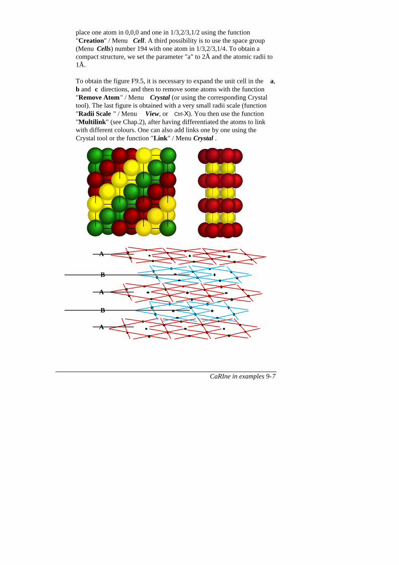
CaRIne in examples 9-7
place one atom in 0,0,0 and one in 1/3,2/3,1/2 using the function"Creation" / Menu Cell. A third possibility is to use the space group(Menu Cells) number 194 with one atom in 1/3,2/3,1/4. To obtain acompact structure, we set the parameter "a" to 2Å and the atomic radii to1Å.
To obtain the figure F9.5, it is necessary to expand the unit cell in the a,b and c directions, and then to remove some atoms with the function"Remove Atom" / Menu Crystal (or using the corresponding Crystaltool). The last figure is obtained with a very small radii scale (function"Radii Scale" / Menu View, or Ctrl-X). You then use the function"Multilink " (see Chap.2), after having differentiated the atoms to linkwith different colours. One can also add links one by one using theCrystal tool or the function "Link " / Menu Crystal .
A
B
A
B
A

CaRIne in examples 9-8
F9.5: ABCABC… stacking in FCC (top left), ABAB… stacking in HCP(top right and bottom).
9.4 Visualisation of the (111) surface of diamond
Question : Visualise the (111) surface of the diamond structure.
Solutions :
First, you have to create a diamond crystal. To do so, we have severalsolutions :
1 - load the diamond cell from the cells library;2 - create the diamond cell from the atomic positions (see §3.5);3 - create the diamond cell from the space group (see §3.6).
The next step consists in expanding the crystal (function "Spread of" /Menu Crystal) to 3*3*3 or 4*4*4 cells in order to better visualise theplanes. The general scale (keys - et +) might need to be changed.
Then, you select the (111) plane (function "Choice of hkl planes " /Menu hkl/uvw). If we give a "thickness" to this plane (E=0.1), we cansee some atoms close to the (111) plane. To visualise this structure, youuse a 20% radii of and you do a projection parallel to a directionbelonging to the (111) plane ([01-1] for example) : function "? [uvw]with mouse", click on two atoms of the (111) plane, and then select"Projection // [uvw].
A nice way to visualise the different layers is to use different colours. Wecan also use the polyhedrons of coordination to show the diamondstructure. We can follow the sequence given below :
1/ create the diamond lattice;2/ using the " Creation" dialogue box / Menu Cells, give a differentcolour to the interstitials3/ expand the crystal;

CaRIne in examples 9-9
4/ cut the crystal with a (111) plane, with E=0.1 (function "Choice ofhkl planes"), make a projection // [01-1];5/ translate this plane (function "Translation + plane 1 ") to obtain amaximum of selected atoms;6/ change the colour of all the atoms of this plane (function "ModifyAtom");7/ ask again for the (111) plane, but this time with E=0, and cross off the"cut option";8/ translate this plane to superpose it to the one selected in 5/;9/ give a new colour to this plane;10/ destroy all hidden atoms (crystal tools);11/ translate again (� B);12/ give a third colour;13/ ask for the coordination polyhedrons from an atom located in thetetrahedral site.
Remark : the polyhedrons take the colour of their central atom.

CaRIne in examples 9-10
F9.6 : Visualisation of the (111) plane of the diamond structure. Projectionperpendicular to the (111) plane (previous page), and projection parallel to
the [0 1 -1] direction.
9.5 X-Rays diffraction : Au-Cu alloys
Question : Compare the X-Rays diffraction patterns of the ordered AuCualloy to the disordered AuCu alloy (50 at% Cu).
Data : Gold (Au) : FCC, a=4.08 ÅCopper (Cu) : FCC, a=3.61 ÅDisordered AuCu alloy : FCC, a=3.84 ÅOrdered AuCu alloy : tetragonal, a=3.98 Å and c=3.72 Å.

CaRIne in examples 9-11
The last structure can be described as a Gold FCC cell, with asubstitution of (002) plane Gold atoms by Copper atoms. Thissubstitution leads to a slight contraction of the c-axis.
Solutions : The aim of this problem is to superpose the X-Ray diffractiondiagrams of an ordered and disordered Au-Cu solid solutions of the samecomposition (50at% Au, 50at%Cu). We will then see additional peaks inthe ordered structure. From the software user point of view, we will alsolearn how to share a same site between different kinds of atoms.
Creation of the unit cells : The Gold, Copper and disordered AuCu alloy
are FCC cells. One solution is then to use the 225 th space group(Fm3 m ) (function "Space Group" / Menu Cell). For the Gold, we placean atom Au at 0,0,0 and we set the "a" parameter to 4,08Å. This cell issaved as "Au Gold Metal Cubic". For the Copper, we use a=3.61Å, andthe cell is saved as "Cu Copper Metal Cubic". For the disordered alloy,the procedure is slightly different. We create two sites in 0,0,0. The firstone is occupied by Au atoms, with an occupancy of 0.5. The second oneis occupied by Cu atoms, with an occupancy of 0.5. This cell is savedunder the name "Au Cu FCC disordered".The ordered alloy can be built from the Gold FCC cell previouslydescribed. We then load the "Au Gold Metal Cubic" and save it with thenew name "AuCu ordered (tetragonal)". In order to modify the a,b and cparameters, and in order to substitute Copper atoms to Gold atoms, weuse the function "Creation" / Menu Cells. Then, we save this again.
X-Rays diffraction diagrams : The first step is to load the two structures(ordered and disordered). Then, we need to associate them. To do so, we"active" the "AuCu FCC Disordered" window by clicking inside. Thenwe select the function "Associated Lattices" from the Menu Specials. Inthe dialogue box which is then opened, we select "AuCu ordered(tetragonal)". Still from the "AuCu FCC disordered" window, we cannow ask for the calculation of the X-Rays diffraction diagrams (function"Create", Menu Specials/RX). Because the two lattices are associated,their diagrams will be superposed. It is possible (and recommended) togive a different pattern and colour to each diagram (see Chap.7). For theresults presented in the following figure, we have used λ=0.1788965 nm(Kα1 Cobalt).

CaRIne in examples 9-12
We can clearly observe the additional peaks for the ordered structure. Wealso observe a difference in the peaks positions due to the difference incell dimensions.
Intensity
2 ΘΘΘΘ
20 30 40 50 60 70 80 900
10
20
30
40
50
60
70
80
90
100
(55.53,45)
200
(82.42,23)
220
(47.59,100)
111
AuCu desordered
Intensity
2 ΘΘΘΘ
20 30 40 50 60 70 80 900
10
20
30
40
50
60
70
80
90
100
(59.41,43)
200
(88.99,20)
220
(50.83,100)
111
Cu
AuCu ordered
Intensity
2 ΘΘΘΘ
20 30 40 50 60 70 80 900
10
20
30
40
50
60
70
80
90
100
(27.60,38)
100(56.99,44)
200
(64.47,13)
210(39.43,29)
110
(84.86,22)
220
(71.50,9)
211
(48.80,100)
111Intensity
2 ΘΘΘΘ
20 30 40 50 60 70 80 90
0
10
20
30
40
50
60
70
80
90
100
(52.01,49)
200
(76.65,33)
220
(44.63,100)
111
Au
Intensity
2 ΘΘΘΘ
20 30 40 50 60 70 80 90
0
10
20
30
40
50
60
70
80
90
100
100200
210
110220
211
111
200
220
111 AuCu desorderedAuCu ordered
disordered
disordered

ASCII File Formats A-1
Appendix AFormat Standard ASCII File andformat of DOS versions files
AThis appendix describes the four file formats whichallow CaRIne to exchange information with othersoftware.
Remark : To get examples of these files, the best way is to build a cell or acrystal with CaRIne and to save it under one of these ASCII file formats.
A-1 "Cell Standard ASCII File"
This format is used to exchange the unit cell descriptions with othersoftware. The files obey to the following structure :
CaRIne Crystallography 3.0 : Name of the application which has created the file.
Cell Standard ASCII File=Diamond.txt : Name of the file.File Version Number=1 :
Colors Referred to : Mendeleev Table : Reference for the colour of atoms. Here, the colour of atoms are given
by the Mendeleev table used by CaRIne.
---------------------- : Beginning of the description of the Cell Definition unit cell, or motif with space group.----------------------
Cell Parameters (Å and °) : Cell parameters in Angstrom (Å) and in degrees (°).
a=3.57 b=3.57 c=3.57
ASCII File Formats A-2
alpha=90.00 beta=90.00 gamma=90.00
System=Cubic : Crystalline system (Cubic, Triclinic, Monoclinic, Orthorhombic, Trigonal, Tetragonal, Hexagonal).
Space Group Number=not used : Space group number (between 1 and 230). "not used" signifies that the space group symmetries
are not used to build the unit cell.
Number of Positions in Cell=8 : Number of positions in the unit cell (if Space Group Number=not
used),or number of non-equivalent atoms of the motif (if Space Group Number≠0)
Atom Oxi. X Y Z R(Å) Occ. Beginning of the position listC Co 0 0 0 0.77 1.0000 For each position, one can read :C Co 1/2 0 1/2 0.77 1.0000 •the chemical symbolC Co 0 1/2 1/2 0.77 1.0000 •the degree of oxidationC Co 1/4 1/4 3/4 0.77 1.0000 ("Co" indicates covalent state)C Co 1/2 1/2 0 0.77 1.0000 •the reduced co-ordinates in theC Co 1/4 3/4 1/4 0.77 1.0000 (a,b,c) reference frameC Co 3/4 1/4 1/4 0.77 1.0000 •the atom/ion radius (in Å)C Co 3/4 3/4 3/4 0.77 1.0000 •the occupation factor
The different colour references
In the preceding example, the colours of the atoms were referred to theMendeleev table used by CaRIne. There are two other possibilities :"RGB Components" and "16 Colours Palette".
• RGB Components :
In this case, there are three supplementary fields for each position : Red,Green and Blue. These three values should belong to the interval[0,65535].
Example :
Atom Oxi. X Y Z R(Å) Occ. Red Green BlueC Co 0 0 0 0.77 1.0000 15528 15528 15528C Co 1/2 0 1/2 0.77 1.0000 2000 2000 2000C Co 0 1/2 1/2 0.77 1.0000 15528 15528 15528C Co 1/4 1/4 3/4 0.77 1.0000 5369 5369 5369C Co 1/2 1/2 0 0.77 1.0000 255 35200 14695C Co 1/4 3/4 1/4 0.77 1.0000 36895 15698 2365C Co 3/4 1/4 1/4 0.77 1.0000 235 2369 14596

ASCII File Formats A-3
C Co 3/4 3/4 3/4 0.77 1.0000 25698 1023 36952
• 16 Colours Palette :
In this case, there is one supplementary field for each position : "Colour".This colour belongs to the following list :
•Black•Blue•Green•Cyan
•Red•Magenta•Brown•Lightgray
•Gray•Lightblue•Lightgreen•Lightcyan
•Lightred•Lightmagenta/Pink•Yellow•White
Unit cell described from the space group
If the "Space Group Number" is different than "not used", then the filemay contain either :
• the list of all positions of the unit cell,or • the list of only non-equivalent positions.
In order to differentiate these two possibilities, a key-sentence should beplaced just after the space group number :
• Only Non Equivalent Positions are listed: for the motif case,• All Positions are listed : for the unit cell case.
• "Only Non Equivalent Positions are listed" example:
Space Group Number=227Only Non Equivalent Positions are listed
Number of Positions in Cell=1
Atom Oxi. X Y Z R(Å) Occ.C Co 1/8 1/8 1/8 0.77 1.0000

ASCII File Formats A-4
• "All Positions are listed" example:
Remark that in this case there is a supplementary field for each position.This field indicates if the position is "equivalent" or not ("Eq." or"NonEq.").
Space Group Number=227All Positions are listed
Number of Positions in Cell=8
Atom Oxi. X Y Z R(Å) Occ.C Co 1/8 1/8 1/8 0.77 1.0000 NonEq.C Co 1/8 5/8 5/8 0.77 1.0000 Eq.C Co 5/8 1/8 5/8 0.77 1.0000 Eq.C Co 5/8 5/8 1/8 0.77 1.0000 Eq.C Co 7/8 7/8 7/8 0.77 1.0000 Eq.C Co 7/8 3/8 3/8 0.77 1.0000 Eq.C Co 3/8 7/8 3/8 0.77 1.0000 Eq.C Co 3/8 3/8 7/8 0.77 1.0000 Eq.
A-2 The "Crystal Standard ASCII File"
This file format is used to exchange crystals files with other sofwares.This format includes the informations relative to the unit cell (see §A.1)and the informations concerning the crystal (spreading, point defects,links, cartesian atomic positions, ...) and the display (orientation, scales,background colour,...).
The first part of the file corresponds to the "Cell Standard ASCII File",then come the informations relative to the crystal :
CaRIne Crystallography 3.0 : Name of the application which has created the file.
Cell Standard ASCII File=Diamond.txt : Name of the file.File Version Number=1 :
Colours Referred to : Mendeleev Table : Reference for the colour of atoms. Here, the colour of atoms are given by the Mendeleev table used by
CaRIne.
---------------------- : Beginning of the description of theCell Definition unit cell, or motif with space group.

ASCII File Formats A-5
----------------------………----------------------Crystal Definition : Beginning of the crystal---------------------- definition.(a,b,c) Frame : : Co-ordinates of the cell
reference frame vectors (a,b,c) in the cartesian orthonormal reference frame Rr (see Chapter 4).
Origin x=0 y=0 z=0 : Origin of the (a,b,c) reference framei x=90.000 y=0 z=0 : Co-ordinates of the vector aj x=-0.000 y=90.000 z=0 : Co-ordinates of the vector bk x=-0.000 y=-0.000 z=90.000 : Co-ordinates of the vector c
(X,Y,Z) Frame : : Co-ordinates of the cartesian ortho-normal reference frame Rr given in the screen reference frame Re (see Chapter 4). This defines the orienta-tion of the crystal relatively to the screen.
Origin x=0 y=0 z=0 : Origin of the (x,y,z) reference framei x=1.000 y=0 z=0 : Vector xj x=0 y=1.000 z=0 : Vector yk x=0 y=0 z=1.000 : Vector z
Spread Of : : Spreading of the crystal.na=1 nb=1 nc=1 : Number of cells in each direction.Build from origin : Key-sentence indicating if the lattice is
expanded from the unit cell origin ("Build from origin") or from the unit cell centre ("Build from centre").
Planes and Direction:(1,0,0), (-1,-1,1), (0,2,-3), [1,1,1] : crystallographic plans and direction indices currently used by CaRIne.
General Scale=30.00 : General scale (between 1 and 2000).Radii Scale=100.00 : Radii scale (in %, real number between
1 and 400).
Graphical Options : : Description of the graphical options :
Perspective= TRUE : Perspective effect.Show Planes= TRUE : Display of atoms belonging to the
selected planes.Show Frame= TRUE : Display of all links between atoms.Show Atoms= TRUE : Display of the atoms.Show Polyhedrons= TRUE : Display of the coordination polyhedrons.Shading Effect= FALSE : Shading effect.

ASCII File Formats A-6
Number of Atoms in Crystal=14 : Number of atoms in the crystal (all atoms, displayed or not).
For each position one can read on a same line :• the reference number of the atom/ion,• its chemical symbol ("*" indicates an unknown chemical symbol),• its degree of oxidation,• its co-ordinates in the cell reference frame (a,b,c),• its co-ordinates in the cartesian reference frame linked to the screen (x,y,z),• its atomic radius,• eventually, the RGB components (see A.1). Here, the colours are referenced to the
Mendeleev table,• a boolean indicating if there is a vacancy on this site,• a boolean indicating if the atom/ion is hidden,• a boolean indicating if the atom/ion belongs to the plane #1,• a boolean indicating if the atom/ion belongs to the plane #2,• a boolean indicating if the atom/ion belongs to the plane #3,
# Atom Oxi i j k X Y Z R(Å) Vacancy Hidden p 1 p 2 p 31 * 1 0 1 45.00000 -45.00000 45.00000 1.00 FALSE FALSE F F F2 * 0 1 1 -45.00000 45.00000 45.00000 1.00 FALSE FALSE F F F3 * 1 1 1 45.00000 45.00000 45.00000 1.00 FALSE FALSE F F F4 * 0 0 1 -45.00000 -45.00000 45.00000 1.00 FALSE FALSE F F F5 * 1/2 1/2 1 -0.00000 -0.00000 45.00000 1.00 FALSE FALSE F F F6 * 1/2 0 1/2 0.00000 -45.00000 0 1.00 FALSE FALSE F F F7 * 0 1/2 1/2 -45.00000 0.00000 0 1.00 FALSE FALSE F F F8 * 1 1/2 1/2 45.00000 0.00000 0 1.00 FALSE FALSE F F F9 * 1/2 1 1/2 -0.00000 45.00000 0 1.00 FALSE FALSE F F F10 * 1/2 1/2 0 0.00000 0.00000 -45.00000 1.00 FALSE FALSE F F F11 * 0 0 0 -45.00000 -45.00000 -45.00000 1.00 FALSE FALSE F F F12 * 0 1 0 -45.00000 45.00000 -45.00000 1.00 FALSE FALSE F F F13 * 1 1 0 45.00000 45.00000 -45.00000 1.00 FALSE FALSE F F F14 * 1 0 0 45.00000 -45.00000 -45.00000 1.00 FALSE FALSE F F F
Number of Links in Crystal=12 : Number of links between atoms in this crystal.
Atom#1 Atom#2 Thickness Colour : Beginning of the list of links.3 1 1 Black2 4 1 Black For each link, we find on the same line :3 2 1 Black1 4 1 Black • the reference number of the first atom,3 13 1 Black • the reference number of the second atom,2 12 1 Black • the thickness of the link,4 11 1 Black • the colour of the link.1 14 1 Black13 12 1 Black The colour of a link can be chosen in the following12 11 1 Black list :14 11 1 Black13 14 1 Black Black,White,Cyan,Magenta,Red,Green,Blue,Yellow

ASCII File Formats A-7
Note : this version (1) of the Crystal Standard ASCII File does not allowthe coordination polyhedrons list to be exported or imported.
A-3 The "Cell DOS File Format"
This format is used by the versions of CaRIne for DOS (1.0 to 2.5) todescribe the unit cells. The signification of each line is given below :
# line Signification
1234567Atome1 (1)Atome1 (2)Atome1 (3)Atome1 (4)Atome1 (5)…
a {Ångstrom}bcalpha {radians}betagammaNumber of atoms in the unit cellx { reduced co-ordinates of the atoms - between 0 and 1}yzradius {Ångstrom}colour {integer between 1 and 16}and so on for all the atoms of the cell...

ASCII File Formats A-8
A-4 The "Crystal DOS File Format"
This format is used by the versions of CaRIne for DOS (2.1 to 2.5) todescribe the crystals. The signification of each line is given below :
The first part of the file corresponds to the unit cell (see §A.3).
# line Signification
1234567Atome1 (1)Atome1 (2)Atome1 (3)Atome1 (4)Atome1 (5)…
a {Ångstrom}bcalpha {radians}betagammaNumber of atoms in the unit cellx { reduced co-ordinates of the atoms - between 0 and 1}yzradius {Ångstrom}colour {integer between 1 and 16, see table A.1}and so on for all the atoms of the cell...
The file continues with the description of the crystal. The value of thevariable X is equal to 7 plus 5 times the number of atoms in a unit cell.
# line SignificationX+1 value of the general scaleX+2 value of the radii scale (in % of full size)
a list of Boolean follows (1=true), corresponding to the state of graphicoptions
X+3 1 = only the atoms of the selected planes /0 = all atomsX+4 1 = reference frame xyzX+5 1 = reference frame abcX+6 1 = frame (connections between atoms)X+7 1 = atoms displayedX+8 1 = direction [uvw]X+9 1 = perspective effectX+10 1 = rapid displayX+11 1 = transparencyX+12 1 = nice display
description of the crystal
X+13 number of unit cells in the a direction (na)

ASCII File Formats A-9
X+14 number of unit cells in the b direction (nb)X+15 number of unit cells in the c direction (nc)
description of the reference frame (x,y,z)
X+16 x0 {co-ordinates of the reference frame origin}X+17 y0X+18 z0X+19 xX {co-ordinates of the vector X}X+20 yXX+21 zX
… same thing for the two other unit vectors
X+28 Description of the abc reference frame (similar to the xyz ref. frame)…
description of the three selected planesX+40 hX+41 kX+42 lX+43 epsilon ("thickness"}X+44 ix {co-ordinates of the translation vector between two successive (hkl)
planes}X+45 iy {in the unit cell reference frame}X+46 izX+47 tx {co-ordinates of the translation vector between the (hkl) plane which is}X+48 ty {the closest to the origin, and the current (hkl) plane}X+49 tz… same thing for the two other planesX+70 u {co-ordinates of the current [uvw] direction}X+71 vX+72 wX+73 number of atoms in the crystal
for each atom
X+74 x {co-ordinates in the (x,y,z) reference frame}X+75 yX+76 zX+77 radiusX+78 colour {integer between 1 and 16, see table A.1}X+79 i {co-ordinates in the (a,b,c) reference frame}X+80 jX+81 kX+82 1 = this atom is displayed, 0 = this atom is hiddenX+83 1 = this atom belongs to the plane number 1X+84 1 = this atom belongs to the plane number 2X+85 1 = this atom belongs to the plane number 3X+86 1 = vacancyX+87 the number of the atom/ion

ASCII File Formats A-10
The following information concerns the existing connections between thedifferent atoms. The value of Y is X + 73 + 14n, where n is the totalnumber of atoms.
# line Signification
Y number of linksY+1…
N° N° {on a same line, identification numbers of the connected atoms}…
0123
BlackBlueGreenCyan
4567
RedMagentaBrownLightgray
891011
GrayLightblueLightgreenLightcyan
12131415
LightredLightmagenta/PinkYellowWhite
Table A.1 : Value of the colour of the EGA palette
0 black 4 blue1 white 5 lightblue2 red 6 pink3 green 7 yellow
Table A.2 : Value of "the 8 colour palette"

Setting the default values with the registry B-1
Appendix BSetting the default values with theregistry
BThis appendix describes all the initialization parametersrecorded in the registry
Modification of the registry
Attention :
All the initialization parameters are recorded in the Windows 95 orNT 4.0 registry. A normal use of CaRIne does not imply to modifythese data. Most of these parameters can be modified inside theapplication itself. CaRIne save the new parameters when closing.Registry modifications should be done only when the option is notavailable in CaRIne.
These parameters are recorded under the following key :
HKEY_CURRENT_USER\Software\CaRIne\3.1
To modify them, use the registry editor of Windows (MenuStart/Run regedit).

Setting the default values with the registry B-2
Details of the registry list
Values in darken lines should not be modified by users as they canprevent CaRIne to work correctly. When modifying the registry,respect the formats : number of values, «space» between characters,...
HKEY_CURRENT_USER\Software\CaRIne\3.1\Crystal
Creation/List=34 123 497 354 85 135 197 263 326 376
Background Color=1
Default background color for a new crystal window (1 for white, 0for black).
abc frame=0 18
Color of the abc reference frame and size of characters. Colors areselected from table A.2.
xyz frame=4 18
Color of the xyz reference frame and size of characters. Colors areselected from table A.2.
Dhkl list=0 5 0 5 0 5
h, k, and l ranges for creation of a list of planes used for the Dhkllist calculation (Calcul | Plane spacing list).
Angle hkl list=-3 3 -3 3 -3 3
h, k, and l ranges for the angle between planes list calculation(Calcul | planes angle list).

Setting the default values with the registry B-3
HKEY_CURRENT_USER\Software\CaRIne\3.1\Directories
CEL=C:\CaRIne 3.1\CellsMTF=C:\CaRIne 3.1\MTFACE=C:\CaRIne 3.1\Cell Standard ASCII File (ACE)CRY=C:\CaRIne 3.1\CrystalsRES=C:\CaRIne 3.1\RESACR=C:\CaRIne 3.1\Crystal Standard ASCII File (ACR)XRD=C:\CaRIne 3.1\Import-ExportPersonal=Personal directory
CaRIne’s librairies directories. To be modified when runningCaRIne (Menu Files | Options).
HKEY_CURRENT_USER\Software\CaRIne\3.1\Reciprocal lattice
delta s=0.020
Maximum reciprocal distance between a node and the reciprocallattice plane when using the Special | Reciprocal Lattice | Zoneaxis function.
Spread=-2 2 -2 2 -2 2
Ranges for the reciprocal lattices (hmin hmax kmin kmax lminlmax).
Background color=1
Default background color for the reciprocal lattice windows(1 : white, 0 : black).
Node color=0
Reciprocal lattice nodes’ color ( to be chosen in table A.2).
Frame color=3
Reciprocal lattice frame’s color ( to be chosen in table A.2).

Setting the default values with the registry B-4
a*b*c* frame=2 18
Color of the abc reference frame and size of characters. Colors areselected from table A.2.
HKEY_CURRENT_USER\Software\CaRIne\3.1\Settings
Language=EnglishBuilding pictures=2 200 1Larger buttons=FALSE
These options are to be modified with the function File | Options.
HKEY_CURRENT_USER\Software\CaRIne\3.1\Stereographic projection
Radii=90
Stereographic projection radius size (in mm) (for the printing).
Direction=-1 1 -1 1 -1 1
Ranges of indices for the directions list creation in Special |Stereographic projection | Parameters (umin umax vmin vmaxwmin wmax).
Pole=-1 1 -1 1 -1 1
Ranges of indices for the planes list creation in Special |Stereographic projection | Parameters (hmin hmax kmin kmaxlmin lmax).
Plane=-1 1 -1 1 -1 1
Ranges of indices for the trace of planes list creation in Special |Stereographic projection | Parameters (hmin hmax kmin kmaxlmin lmax).

Setting the default values with the registry B-5
HKEY_CURRENT_USER\Software\CaRIne\3.1\Tools
General=0 0Crystal=0 0StereoProj=0 0Rotations=878 544Demo=0 0
HKEY_CURRENT_USER\Software\CaRIne\3.1\X-Ray Diffraction
Domain=0 60
Calculation domain of Bragg’s angle for the XRD diagrams (in°).
Temperature factor=1.0
Isotropic temperature factor B.
Step=0.1
Mini intensity=1.00
Minimum intensity for the peaks to be indexed.
Integral breadth=0.1
Integral width of the XRD peaks (to be modified with the functionView | Graphics).
Don't show peaks as sticks=TRUE
To be modified with the function View | Graphics.
Show envelope for each diagram=TRUE
To be modified with the function View | Graphics.
Show sum=TRUE
To be modified with the function View | Graphics.

Setting the default values with the registry B-6
Sum style=4 3
Color and style of the XRD peaks sum lines (see table A.2).
Background Color=1
Defaults background color of XRD window (1 : white, 0 : black).
Grid color=2
XRD grid color (see table A.2).
Axis-Legend color=0
Default axis and legend colors for the XRD diagrams (see tableA.2).

Diffusion factors for the atoms/ions C-1
Appendix CDiffusion factors for theatoms/ions
CThis is the list of atoms and ions differenciated by CaRIne when dealing with theirdiffusion factors as a fonction of sin θ/λ :
H H- He Li Li+ Be
Be2+ B C C2+- N O
O- F F- Ne Na Na+
Mg Mg2+ Al Al3+ Si Si2+-
Si4+ P S Cl Cl- Ar
K K+ Ca Ca2+ Sc Sc3+
Ti Ti2+ Ti3+ Ti4+ V V2+
V3+ V5+ Cr Cr2+ Cr3+ Mn
Mn2+ Mn3+ Mn4+ Fe Fe2+ Fe3+
Co Co2+ Co3+ Ni Ni2+ Ni3+
Cu Cu+ Cu2+ Zn Zn2+ Ga
Ga3+ Ge Ge4+ Tb Tb3+ Dy
Dy3+ Ho Ho3+ Er Er3+ Tm
Tm3+ Yb Yb2+ Yb3+ Lu Lu3+
Hf Hf4+ Ta Ta5+ W W6+
Re Os Os4+ Ir Ir3+ Ir4+
Pt Pt2+ Pt4+ Au Au+ Au3+
Hg Hg+ Hg2+ Tl Tl+ Tl3+
Pb Pb2+ Pb4+ Bi Bi3+ Bi5+
Po At Rn Fr Ra Ra2+
Ac Ac3+ Th Th4+ Pa U
U3+ U4+ U6+ Np Np3+ Np4+
Np6+ Pu Pu3+ Pu4+ Pu6+ Am
Cm Bk Cf As Se Br
Br- Kr Rb Rb+ Sr Sr2+
Y Y3+ Zr Zr4+ Nb Nb3+
Nb5+ Mo Mo3+ Mo5+ Mo6+ Tc

Diffusion factors for the atoms/ions C-2
Ru Ru3+ Ru4+ Rh Rh3+ Rh4+
Pd Pd2+ Pd4+ Ag Ag+ Ag2+
Cd Cd2+ In In3+ Sn Sn2+
Sn4+ Sb Sb3+ Sb5+ Te I
I- Xe Cs Ba Ba2+ La
La3+ Ce Ce3+ Ce4+ Pr Pr3+
Pr4+ Nd Nd3+ Pm Pm3+ Sm
Sm3+ Eu Eu2+ Eu3+ Gd Gd3+

How to use the list generators D-1
Appendix DHow to use the list generators D
This appendix describes how to obtain a list ofplanes or directions using the list generators.
These generators can be found in the following functions :
• "Planes spacing (list)" of Menu Calcul,• "Plans angle (list)" of Menu Calcul,• "Parameters" of Menu Special/Stereo Proj.
A "list generator" is composed of :
Creates an indice list fromthe range given here oneach variable : u,v,w,h,k or
"Add" button
Edit box toenter newindices
List of indices forthe planes or thedirections
"Add a form ofplanes" button

How to use the list generators D-2
• One button to open the dialog box in whichranges are given.
• One field to enter new plane/direction one by one (values areseparated with "," (commas)).
• One button to add the element corresponding to the
previous field. • One button to add a form of planes generated from the
element corresponding to the previous field (only available forplanes, not for directions).
• A context menu in order to : Remove all elements,
Import/Export a list of elements from/to a text file. Click onthe list box with the mouse (right button) to open this contextmenu :
• A list of all elements.
It is possible to move in a list with the keys : , . You can then
select one element and delete it with the del (del) key of your keyboard
(or double-click).
When a form of planes is generated, CaRIne opens a dialog box whereplanes can be selected or unselected before being added in the list ofelements.
Index i
Index i-1
(hkl) : see planes[uvw] : see directions2D : I-5; 2-83D : 2-8
Aabsorption, factor : 7-3accelerating voltage : 2-25;9-2angle
• of diffraction : see "Bragg's angle"• solid angle : 2-29
Angstrom : I-7association of lattices : 2-35; Chap-5atomic number : 3-12axis
• of rotation : 2-48; Chap-4• of a zone, zone axis :1-7; 2-27,24;
8-6,7;9-2,3
Bbeam
• transmitted beam : 2-24Bragg's angle : 2-23; 7-1Bragg's geometrical configuration : 7-1Bravais's Lattices
• creation : I-2; 2-13;3-2,3• definition : 3-2• use of : 3-2
CCauchy : 7-9cell, unit cell
• creation : 2-13; 3-4• definition : I-1• fi les : 2-8,9,10; 3-1• multiplication : 2-36Cell Standard ASCII file :2-9,10;
Appendix Acentre of rotation : 2-48chemical symbol : 2-38…2-41,45; 3-5,12clipboard: 2-12constant of camera : 2-25,26;9-2conversion 3 -> 4 indexes : I-5coordination : see "polyhedron"colour
• of background : 3-2,3,6; 4-6• of an atom : 2-39,40 ; see Periodic
table of the elements• of a link : 2-41,44• of a stereographic projection : 6-4• of a XRD diagram : 7-5
copy : 2-12covalent : 3-12crystal
• definition : 1-1,2• files : 2-8,9,10; 3-1
Crystal Standard ASCII file : 2-9,10; Appendix A
crystalline system : 3-2,6,9

Index i-2
cut• of a crystal : 2-16,17• of a reciprocal lattice : see "Zone
axis"• by a plane : 2-16
Ddefault values : Appendix Bdefects
• in crystals : I-6; 2-39• punctual : I-6; 2-40,41
density• of a plane : 2-18• of a cell : 2-21
dephtshading : 4-6delta S : 8-7;B-3diagram
• x-ray diffraction : 2-34; Chap.7• experimental : 7-6• reference : 7-8• envelope : 7-9
diamond : 2-32; 3-7diffraction
• x-ray diffraction : see "XRD"• electronic diffraction : 2-24;9-1
diffusion factor : Appendix Cdirection, [uvw] direction
• choice : 2-18• current : 2-19• definition : I-4
directory : 0-4directories : 0-5dislocations : I-6; 2-39distance
• between 2 atoms : 2-20,43• interplanar : 2-22
DOS version : 2-9drag and drop : 0-5
EExamples : Chap.9environment of an atom
• successive shells: 2-29• coordination polyhedrons : 2-32• "R.D.F." : 2-31• "Spheres" : 2-21
envelope : 7-9;B-5Epitaxy : 5-5…7error, numerical errors, precision : 2-21; 3-4exportation : 2-9; Appendix A
• WMF : 2-8• Calculus : 2-22,23,26• Stereographic projection : 6-5• XRD : 7-5
Ffactor
• absorption factor : 7-3• atomic scattering factor : 7-2• diffusion factor : Appendix C• Lorentz factor : 7-2• multiplicity factor : 7-3• occupancy factor : 7-2• polarisation factor : 7-2• structure factor : 7-2; 8-2• temperature factor: 7-3;B-5
film : 5-1form of planes : Appendix Dframe (crystal) : 4-6frame (reference) :
• screen : 4-1• (a,b,c) : 4-1; B-2• (a*,b*,c*) : 8-1;B-4• (x,y,z) : B-2
Frenkel defect : 1-6

Index i-3
Ggraphite : 2-43grain boundary : 1-6"Graphics": 4-5;6-10;7-9;8-9
HHermann-Mauguin : 3-9hexagonal : 3-2, I-5
Iidentification of planes
• use : 2-24• example : 9-1
importation : 2-8,9;7-6,7indexation of SAD: 2-24indexes
• Miller 's indexes : I-5Install procedure : Chap-0integral breadth, width : 7-9; B-5intensity : 2-22;7-20
• mini : B-5interstitial : 1-6
JJCPDS : 1-7
Llabels : 2-38,39,45language : 2-11;0-4links : 2-41...44libraries : 3-1level of oxidation : see oxidationlaw
• addition law: 8-4• Weiss law: 8-4
length
• wave : 2-25,26• camera : 2-25,26
Lorentz factor : 7-2
Mmatrix : 2-35; Chap-5Mendeleev : see Periodic table of theelementsMiller : see indexesMolecular dynamics : 2-9motif
• creation : 2-13• definition : 1-1...3• fi les : 2-8; 3-1; Appendix A
multiplicity : 7-3
NNaCl : 3-4network : 0-4node
• of the real lattice: 1-1• of the reciprocal lattice : 8-2; B-3
Ooccupancy : 3-4,5; 7-2orientation
• using Miller indices : 4-2• using the keyboard : 4-2• using the mouse : 4-3; 8-2• using the stereographic projection :
4-4;6-9,10• using the reciprocal lattice : 8-1,7• using the Rotation tools : 4-4
organic molecule : 2-40oxidation : 2-38...40,45;3-5,11,12
P

Index i-4
parameters, cell parameters : 1-1,2;3-3paste : 2-12Periodic table of the elements : 2-39,40
• access : 3-2…6• use : 3-11
perspective• of a crystal : 4-6• of the reciprocal lattice : 4-9
personal directory : 0-4,5planes, (hkl) planes
• show : 4-6• selection : 2-15• translation : 2-16,18; 4-5
plane spacing : 2-22; 8-8polarisation factor : 7-2pole : 6-2…6polyhedron : 2-32,33,44,45precipitate : 1-6; 2-35; Chap.5precision, numerical precision : 3-4printing : 2-11projection (crystallographic) : 2-18,19punctual groups : I-3
Rradii :
• scale : see scale• stereographic proj. :B-4
real lattice, direct lattice• definition : I-1• spread of : 2-36
reciprocal lattice• creation : 2-35; 8-6• definition : 8-1• spread of : 8-6
RDF (radial distribution function) : 2-31reference frame :
• screen : 4-1• (a,b,c) : 4-1• (a*,b*,c*) : 8-1
"Refresh" (window) : 2-49Registry : Appendix Brelation of epitaxy : 2-35; 5-4...7relaxation : 2-39rolling sheet: 2-33rotations
• using keyboard or mouse : Chap.4.2• continuous : 2-47• parameters : 2-47• using the reciprocal lattice : 8-1;7• using the stereographic projection :
4-4;6-9,10rotation step: 2-47
SScale
• radii scale : 2-46,47;8-2• general scale : 2-46,47; 4-4;8-2• XRD : 7-10
Schoenflies : 3-9Schottky : 1-6shading : 4-7shell
• environment of an atom : 2-29solid angle : 2-29space group number : 3-9space groups
• definition : I-3,4• use : 2-13; 3-9
spread• of crystal : 2-36• of reciprocal lattice : 8-6; B-3
status bar : 2-2,3stacking (of planes) : 2-40;

Index i-5
stereographic projection• creation : 2-34; 6-2• introduction : 6-1• parameters : 6-3
substitution : 2-39substrat : 5-1superposition
• of the stereographic projections : 5-3
• of the x-ray diffraction diagrams :5-4
system requirements : 0-2
Ttexture : 2-33thickness
• of a plane : 2-15,16• of a link: 2-41,44
"Tile" : 2-50tool palettes : 2-5
• for the stereographic projection :2-50
• for the crystal : 2-49• for rotations : 2-50
trace of a plane : 6-2,4,6translations
• of planes : 2-16,18; 4-5• lattice translations : 1-1,2; 2-14
transmitted beam : 2-24twin boundary : 1-6
Uundo : 2-12units : I-7
Vvacancy : 1-6; 2-41
values (default values) : Appendix Bvolume (unit cell) : 2-21
WWeiss (law of) : 8-4Window
• Crystal windows: 2-1• Stereographic projection
windows : 2-3• Reciprocal lattice windows: 2-4• XRD windows: 2-5• Tool palette windows : 2-5,49...51
WMF (Windows Meta File) : 2-8
XXRD (X-ray diffraction) : Chap.7
• creation : 2-34; 7-4• import experimental file : 7-6• import reference file : 7-8• mixture : 7-4
ZZone axis : 1-7;2-27;8-6,7;9-2,3

Index i-6

Technical Assistance
CaRIne Crystallography17, rue du Moulin du RoyF-60300 SENLISFRANCE
� / Fax : (+33) 3 44 53 44 67 (Attention : C. Boudias)
e-mail : [email protected]@enciacet.fr