carbon accounting of forest bioenergy: from model calibrations
TRANSCRIPT

1
Carbon accounting of forest bioenergy: from model
calibrations to policy options
The Transatlantic Trade in Wood for Energy: A Dialogue on Sustainability Standards and GHG Emissions
October 23-24, 2013, Savannah Georgia
Patrick Lamers

2
Outline
• Carbon debt– Concept– Modeling options– Example: South-Eastern US studies
• Options to deal with carbon debt– Policy options– Industry options– Conclusions

33
Carbon debt
ConceptModeling options

4
The question
• Time lag and volume of (pulse) emissions from biogenic C release and thus the overall climate mitigation potential of bioenergy
• Not whether biogenic C released during combustion is taken up again via forest growth� sustainable forestry is a prerequisite!

Modeling options
Framework choices
1.Reference point2.Spatial boundary: stand vs. landscape (LS)3.Empirical vs. theoretical forest inventory data: dynamic vs. fixed LS4.Forest C vs. whole LCA5.Displacement effects6.C accumulation vs. climate dynamics7.Albedo effect
Scenario assumptions
and parameterization
5

Framework choices
1. Reference point
• Defines a timelag• Definition important• Terminology varies• Currently most common:
• Payback: the time until the site reaches its pre-harvest carbon level
• Parity: the time until the site reaches the same carbon volume as the reference scenario (e.g. protection)
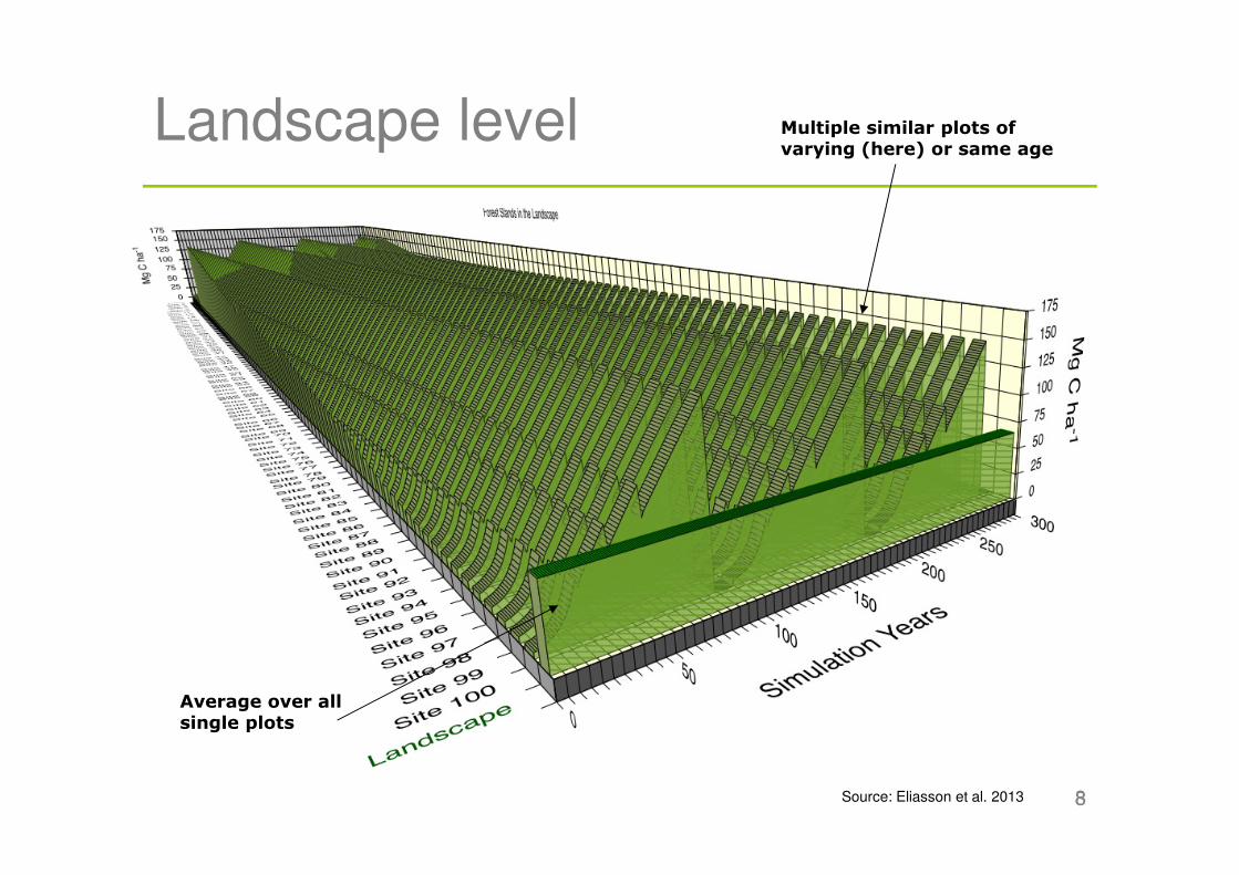
2. Stand vs. Landscape
• Single plot• Only one scenario at any
given time• The baseline remains static
• Multi plot• Bundle of possible harvest
plots (fixed or dynamic)• Scenario applied to one
patch; other plots continue growing or releasing carbon (decay)
6

77
Stand level: single plot
Source: Eliasson et al. 2013
8
Landscape level
8
Multiple similar plots of varying (here) or same age
Average over all single plots
Source: Eliasson et al. 2013

99
Time (years)
Carbon density
(Mg C ha-1)
Carbon break-even points Carbon parity point
Carbon debt1
Harvest scenario
Protection scenario(Baseline)
tbe1tpy
Cdebt2tbe2
Carbon payback time: tbe1 + tbe2 - x
x
1. Harvest 2. Harvest
Typical stand level C balance

1010
Time (years)
Carbon debt
tbetpy
Carbon break-even point Carbon parity point
Carbon density
(Mg C ha-1)
Compare e.g. to : Mitchell et al. 2012
Harvest scenario
Protection scenario(Baseline)
Typical landscape C balance

Modeling options
Framework choices
1.Reference point2.Spatial boundary: stand vs. landscape (LS)3.Empirical vs. theoretical forest inventory data: dynamic vs. fixed LS4.Forest C vs. whole LCA5.Displacement effects6.C accumulation vs. climate dynamics7.Albedo effect
Scenario assumptions
and parameterization
11

5. Displacement effects
• Market mediated effect (demand-supply interrelation)
• Regional, supra-regional, global
• Competition for fiber may result in competition for land (and thus land use change)
12Graph: Pöyry in Dehue 2013

6. C accumulation vs. climate dyn.
• Typically: Cumulative CO2 emissions � C fluxes without climate responses
• Impulse response functions (IRF) – Desribe the atmospheric decay of a pulse emission– Important to understand the climate response to pulse
emissions – Can be used to describe temperature responses
• Additional measures / indicators: – GWPbio: Global Warming Potential (biomass)– (I)GTP: (Integrated) Global Temperature Change Potential
Literature: Cherubini et al. 2011, 2012, 2013; Joos et al. 2012; Peters et al. 201113

6. C accumulation vs. climate dyn.
• Typically: Cumulative CO2 emissions � C fluxes without climate responses
• Impulse response functions (IRF) – Desribe the atmospheric decay of a pulse emission– Important to understand the climate response to pulse
emissions – Can be used to describe temperature responses
• Additional measures / indicators: – GWPbio: Global Warming Potential (biomass)– (I)GTP: (Integrated) Global Temperature Change Potential
Literature: Cherubini et al. 2011, 2012, 2013; Joos et al. 2012; Peters et al. 201114

7. Albedo effect
• Surface albedo: reflection coefficient describing thediffuse reflectivity of a surface
Source: Cherubini et al. 201315

Modeling options
Framework choices
1.Reference point2.Spatial boundary: stand vs. landscape (LS)3.Empirical vs. theoretical forest inventory data: dynamic vs. fixed LS4.Forest C vs. whole LCA5.Displacement effects6.C assumulation vs. climate dynamics7.Albedo effect
Scenario assumptions
and parameterization
1.Energy counterfactual2.Forest baseline 3.Forest assortment 4.Forest biome
16

Parameterization I
1. Energy counterfactual
• GHG counterfactual!• Direct replacement vs.
grid mix?• (Supra-) National vs.
Regional?
2. Forest baseline
• No harvest?• Protection? • In-/excluding wildfire? • Pulp and paper harvest? • Other?�Depends on (regional)
economics at harvest�Varies over time! �Not static!
17

Parameterization II
3. Forest assortment
• Large variety of sourcing areas and feedstock
• US SE: pine thinnings, residues (e.g. tops)
• BC: residues, MPB• Russia: commercial
forestry residues, e.g. aspen
• …
4. Forest biome
• Natural biogenic productivity
• Management adaptation (e.g. fertilization)
• Site sensitivity, e.g. regarding slash removal
18

1919
Example
South-Eastern US analyses

The case study area
• Loblolly pine plantations • Planted post 1950 to
generate fiber for timber, pulp & paper
• Rotation time: 25-35 yrs• Timber & housing market
low since 2008• Increased thinning to save
timber value• Thinnings for P&P and wood
pellet production (~25% of total harvest volume)

Three studies – three outcomes
21
Study Galik & Abt 2012 BERC 2013 Jonker et al. 2013
Region VA, USA South-East USA GA, USA
Model FORCARB Combination GORCAM
Biome: tree species Temperate southern: pure Loblolly pineTemperate southern:
8 different forest type groups Temperate southern: pure Loblolly pine
Assumed age at initial harvest point 22 Inventory data (0- ~130) 20
Rotation [years] 22 dynamic 20
Initial land conversion Managed to managed forestManaged to managed forestNatural to managed forest Managed to managed forest
Harvest share for bioenergy Whole-trees Whole-trees Whole-trees
Methodology/Framework Dynamic landscape Dynamic landscape Stand- and fixed landscape
Forest data Geospatially explicit Geospatially explicit Representative, theoretical plots
Applicability/Biomass use Real case, local use Real case, local use and export Real case, export only
Post-harvest carbon cycling Yes Yes Yes
Full LCA No Yes Yes
Forest baseline Protection: no management / use BAU (timber only harvest) Protection: no harvest, natural regrowth
Energy counterfactual - Fossil electricity (several) Fossil electricity (hard coal)
Displacement modelingYes: e.g. shift in forest area, type,
management intensity Yes: dynamics regarding pulpwood use e.g. Indirect: shift in management insensity
Carbon payback(reference: pre-harvest C level)
Managed forest: 36 yearsProtection reference: 71 years -
4-10 (stand)10-20 (extended stand),< 2 years (landscape)
Carbon Parity (reference: counterfactual) - 35-50 years 12-46 years
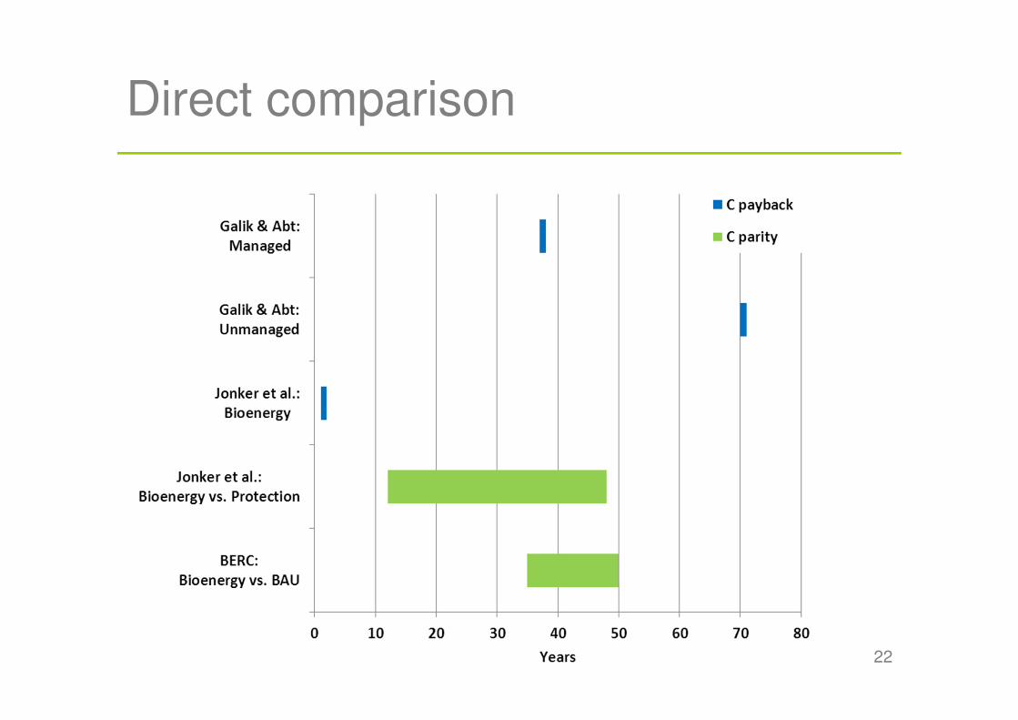
Direct comparison
22

2323
Options to deal with carbon debt
Policy optionsIndustry options
Conclusions

Policy options to deal with C debt
• ‘Panic’ option: black list (feedstock, region, etc.)
���� Fundamental: requirement for sustainable forest management (SFM), i.e. replanting, site monitoring, etc.
24
• ‘Proper’ option: regional indicators (biome & forest assortment specific)

More policy and industry options
Policy level
• Incentivize the use of marginal and unused land
• Increase forest productivity (output)
• Increase supply chain efficiency (avoid losses)
• Integrate fiber production for energy and material (industrial ecology): cascading, residue utilization
Industry / project level
• Establish new plantations on degraded/C-poor land� carbon credit
• Increase forest productivity (e.g. fertilizer, weed control) within SFM limits
• Increase initial number of seedlings, early stand density, and the use of pre-commercial thinnings
25
Conclusions
• Biogenic carbon cycle vs. fossil emissions• Sustainable forest management (for
multiple purposes) is fundamental• No single correct C debt accouting method • Current C debate pays little attention to
forestry economics & climate dynamics• Policy options should be carefully weighed
and regarded in the wider climate mitigation (policy) context
26
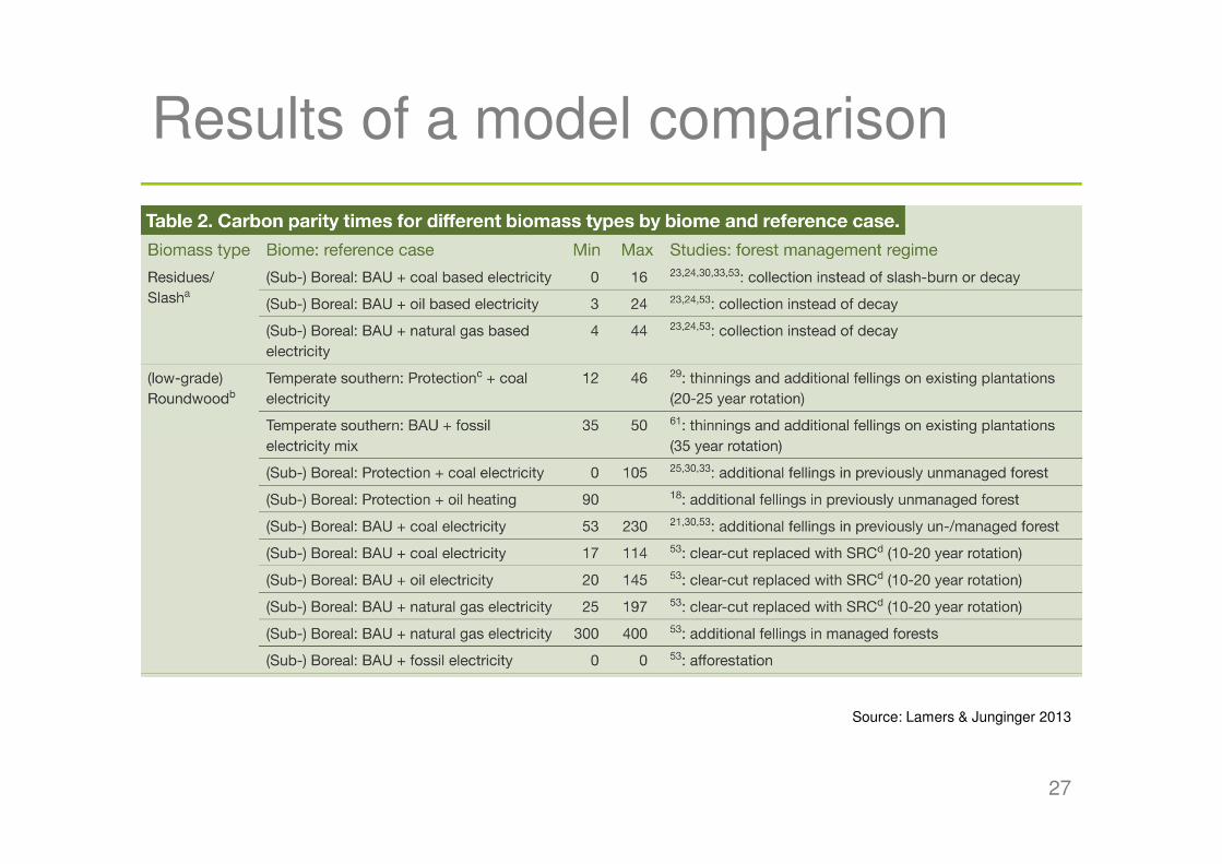
Results of a model comparison
27
Source: Lamers & Junginger 2013

C debt influencing factors
28
Source: Lamers & Junginger 2013

References
29
• BERC (2012) Biomass supply and carbon accounting for southeastern forests. (eds Colnes A, Doshi K, Emick H, Evans A, Perschel R, Robards T, Saah D, Sherman A), Montpelier, VT, USA, Biomass Energy Resource Center, Forest Guild, Spatial Informatics Group.
• Cherubini F, Peters GP, Berntsen T, Stromman AH, Hertwich E. CO2 emissions from biomass combustion for bioenergy: atmospheric decay and contribution to global warming. GCB Bioenergy3(5):413-26 (2011).
• Cherubini F, Bright RM, Stromman AH. Site-specific global warming potentials of biogenic CO2 for bioenergy: contributions from carbon fluxes and albedo dynamics. Environmental Research Letters 7(4):045902 (2012).
• Cherubini F, Guest G, Strømman AH. Application of probability distributions to the modeling of biogenic CO2 fluxes in life cycle assessment. GCB Bioenergy 4(6):784-98 (2012).
• Cherubini F., Bright R. M., Strømman A. (2013) Global climate impacts of forest bioenergy: what, when and how to measure? Environmental Research Letters, 8.
• Dehue, B. (2013). GHG accounting of forest bioenergy . JRC Workshop, Arona, Italy. • Eliasson P., Svensson M., Olsson M., Ågren G. I. (2013) Forest carbon balances at the landscape
scale investigated with the Q model and the CoupModel – Responses to intensified harvests. Forest Ecology and Management, 290, 67-78.
• Galik C. S., Abt R. C. (2012) The effect of assessment scale and metric selection on the greenhouse gas benefits of woody biomass. Biomass and Bioenergy, 44, 1-7.
• Harper, R. & Turner, J. (2013). Wood Supply – Where’s the Pulpwood? (Potential Diameter-class Imbalance in Southern Pines). Forest Bioenergy Conference, USDA Forest Service.

References
30
• Jonker G.-J., Junginger M., Faaij A. (2013) Carbon payback period and carbon offset parity point of wood pellet production in the Southeastern USA. GCB Bioenergy, in press.
• Joos F, Roth R, Fuglestvedt JS, Peters GP, Enting IG, von Bloh W, et al. Carbon dioxide and climate impulse response functions for the computation of greenhouse gas metrics: a multi-model analysis. Atmospheric Chemistry & Physics Discussions 12(8):19799-869 (2012).
• Lamers P., Marchal D., Heinimö J., Steierer F. (forthcoming) Woody biomass trade for energy. In: International Bioenergy Trade: History, status & outlook on securing sustainable bioenergy supply, demand and markets. (eds Junginger M, Goh CS, Faaij A) pp Page. Berlin, Springer.
• Lamers P., Junginger M. (2013) The ‘debt’ is in the detail: a synthesis of recent temporal forest carbon analyses on woody biomass for energy. Biofuels, Bioproducts and Biorefining, 7, 373-385.
• Mitchell S. R., Harmon M. E., O'Connell K. E. B. (2012) Carbon debt and carbon sequestration parity in forest bioenergy production. GCB Bioenergy, 4, 818-827.
• Peters GP, Aamaas B, T. Lund M, Solli C, Fuglestvedt JS. Alternative “Global Warming” Metrics in Life Cycle Assessment: A Case Study with Existing Transportation Data. Environmental Science & Technology 45(20):8633-41 (2011).
