car-to-x communication in heterogeneous environments
TRANSCRIPT

Car-to-X Communication inHeterogeneous Environments
—
Fahrzeug-Umfeld-Kommunikationin heterogenen Szenarien
Der Technischen Fakultät der
Universität Erlangen-Nürnberg
zur Erlangung des Grades
D O K T O R - I N G E N I E U R
vorgelegt von
Christoph Sommer
Erlangen – 2011

Als Dissertation genehmigt von
der Technischen Fakultät der
Universität Erlangen-Nürnberg
Tag der Einreichung: 30. März 2011
Tag der Promotion: 06. Juni 2011
Dekan: Prof. Dr.-Ing. Reinhard German
Berichterstatter: Prof. Dr.-Ing. Falko Dressler
Prof. Ozan K. Tonguz, Ph.D.

Abstract
The challenge of designing and evaluating an integral wireless communication
system that affords the exchange of data between cars and with infrastructure is
commonly answered only in part. Car-to-X communication systems are generally
treated as operating either only in freeway scenarios or only in urban scenarios,
operating either in a completely infrastructure-less or an infrastructure-dependent
fashion. It can be argued, however, that in the highly heterogeneous environments
of real-life deployments such distinctions cannot be made.
In the first part of this work, we demonstrate how to take simulative performance
evaluation of Car-to-X communication systems one step beyond current approaches:
we present our successful Open Source framework Veins for the co-simulation of com-
munication networks and road traffic. It allows simulating complex heterogeneous
scenarios with a high degree of realism and allows for road traffic to be influenced
by network communication – a prerequisite for the evaluation of Traffic Information
System (TIS) designs. Veins relies on a coupling of state-of-the-art simulators from
both domains to incorporate validated models for road traffic microsimulation and
network simulation, and extends them for the simulative performance evaluation of
Car-to-X communication systems.
In a second part of this work, we present our Adaptive Traffic Beacon (ATB)
protocol, an evolved beaconing approach to Car-to-X communication for operation
in truly heterogeneous environments. We base its design on lessons learned from
evaluating common approaches to Inter-Vehicle Communication (IVC), identifying
adaptivity as the key property such approaches were lacking. ATB realizes a self-
organizing TIS also able to make use of optionally available Roadside Unit (RSU)
deployments or a Traffic Information Center (TIC). ATB continuously adapts to
sensed network conditions by adjusting the interval between two beacons to utilize
all unused capacity of the wireless channel, but never more. We demonstrate that,
this way, for high-priority access to the medium and co-existant other protocols and
systems, the channel appears virtually unloaded at all times. We conclude this work
with an evaluation of the strengths and weaknesses of ATB when compared with
state-of-the-art hybrid multi-hop flooding and disruption tolerant networking.
1


Kurzfassung
Der Herausforderung, ein integrales System zum drahtlosen Austausch von Daten
zwischen Fahrzeugen und mit Infrastruktur zu entwerfen und seine Leistung zu be-
werten, stehen üblicherweise lediglich Teillösungen gegenüber. So legt man Ansätze
zur Fahrzeug-Umfeld-Kommunikation entweder für den Einsatz auf Autobahnen
oder aber in Städten, sowie entweder voll abhängig oder unabhängig von dedizierter
Infrastruktur, aus. Allerdings erscheint eine Unterscheidung dieser Klassen vor dem
Hintergrund teils stark heterogen geprägter Einsatzszenarien oft unmöglich.
Im ersten Teil dieser Arbeit wird deshalb ein Ansatz zur simulativen Leistungsbe-
wertung dieser Systeme vorgestellt, der die Co-Simulation von Netzwerk- und Stra-
ßenverkehr erlaubt. In Form des erfolgreichen Open-Source-Simulationswerkzeugs
Veins unterstützt der vorgestellte Ansatz die realitätsnahe Simulation komplexer
heterogener Szenarien, nicht zuletzt auch durch die Modellierung der Rückwirkung
von Netzwerk- auf Straßenverkehr. Veins greift auf die Kopplung zweier etablierter
Werkzeuge zurück, und integriert damit validierte Modelle zur Simulation von Fahr-
zeugbewegung wie auch von Netzwerkverkehr, die jeweils um Funktionalität zur
Bewertung von Ansätzen zur Fahrzeug-Umfeld-Kommunikation erweitert wurden.
Im zweiten Teil dieser Arbeit wird mit ATB ein neuartiges Protokoll zur Verbrei-
tung von Informationen per periodischem Broadcast vorgestellt, das speziell mit
Augenmerk auf die Heterogenität realistischer Szenarien entworfen wurde. Auf-
bauend auf bei der Evaluation existierender Ansätze gewonnenen Erfahrungen, die
immer wieder deren mangelhafte Adaptivität aufzeigte, gelang es, ein selbstorgani-
sierendes Verkehrsinformationssystem, das optional auch Infrastrukturkomponenten
integrieren kann, zu entwickeln. Ferner ist ATB in der Lage, durch die kontinuierli-
che Anpassung des Broadcast-Intervalls lediglich ungenutzte Kanalkapazität – diese
allerdings vollumfänglich – auszunutzen. Dadurch steht dem Versand hochpriorer
Nachrichten, wie auch zeitgleich betriebenen Protokollen, jederzeit freie Kanalka-
pazität zur Verfügung. Den Abschluß der Arbeit bildet eine umfassende Bewertung
von ATB, insbesondere im direkten Vergleich mit komplementären Ansätzen zur
Fahrzeug-Umfeld-Kommunikation.
3

Contents
1 Introduction 7
1.1 Heterogeneity in Car-to-X Communication . . . . . . . . . . . . . . . . 9
1.2 Contribution . . . . . . . . . . . . . . . . . . . . . . . . . . . . . . . . . 11
2 Fundamentals 13
2.1 Network Simulation . . . . . . . . . . . . . . . . . . . . . . . . . . . . . 17
2.2 Road Traffic Simulation . . . . . . . . . . . . . . . . . . . . . . . . . . 25
2.3 Wireless Communication . . . . . . . . . . . . . . . . . . . . . . . . . . 35
2.4 Paradigms and Protocols . . . . . . . . . . . . . . . . . . . . . . . . . . 43
3 Simulating Car-to-X Communications 53
3.1 The Veins Simulation Framework . . . . . . . . . . . . . . . . . . . . . 57
3.2 Performance Metrics . . . . . . . . . . . . . . . . . . . . . . . . . . . . 67
3.3 Signal Propagation and Shadowing . . . . . . . . . . . . . . . . . . . . 75
3.4 Road Networks . . . . . . . . . . . . . . . . . . . . . . . . . . . . . . . 87
3.5 The Impact of Car-to-X Communication . . . . . . . . . . . . . . . . . 93
3.6 Conclusion . . . . . . . . . . . . . . . . . . . . . . . . . . . . . . . . . . 103
4 Engineering Car-to-X Protocols 105
4.1 Deploying MANET Protocols in VANETs . . . . . . . . . . . . . . . . . 111
4.2 IVC Systems Based on Cellular Networks . . . . . . . . . . . . . . . . 123
4.3 The Adaptive Traffic Beacon (ATB) Protocol . . . . . . . . . . . . . . . 141
4.4 Design and Characteristics of ATB . . . . . . . . . . . . . . . . . . . . . 145
4.5 Performance Evaluation of ATB . . . . . . . . . . . . . . . . . . . . . . 153
4.6 Comparison of ATB with Flooding/DTN . . . . . . . . . . . . . . . . . 163
4.7 Conclusion . . . . . . . . . . . . . . . . . . . . . . . . . . . . . . . . . . 167
5 Conclusion 169
Bibliography 187
5


Chapter 1
Introduction
The use of Car-to-X communication, i.e., the exchange of data between cars and with
infrastructure, for improving driving safety and efficiency has been on the mind of
researchers since at least the often-cited 1939 New York World’s Fair [95]. Here, in
its Futurama exhibit, General Motors revealed utopian visions of what highways and
cities might look like twenty years later. In fact, many of the visions showcased there,
as well as in the exhibit designer’s 1940 book Magic Motorways [16], such as that
“car-to-car radio hook-up might be used to advise a driver nearing an intersection
of the approach of another car or even to maintain control of speed and spacing of
cars in the same traffic lane”, are still being pursued today.
A huge number [81] of research projects have since then been undertaken which
tried to make visions of Intelligent Transportation Systems (ITS) a reality. Among the
most notable of research initiatives were the Japan CACS project (1973–1979), the
European Prometheus project (1986–1995), or the U.S. PATH project (1986–1992).
(a) infrared senderat a traffic light
(b) infrared receiver mounted on rear-view mirror of an equipped vehicle
(c) traffic light phases and speed recom-mendation shown in the vehicle
Figure 1.1 – Concept of the 1983 Wolfsburger Welle demonstration project: in-frastructure-to-car communication based on infrared transceivers is employedto transmit traffic light phase information to oncoming vehicles; source: [207].
7

8 1 Introduction
The majority of these initiatives led to working prototypes and successful field
operational tests (Figure 1.1 gives an impression of their level of sophistication);
yet, commercial success failed to match the projects’ promises.
A possible explanation for this can be found in [26]: early approaches were sim-
ply too visionary for their time, commonly focusing on infrastructure-less solutions,
which could not be supported by current technology. The 1980s then saw a shift of
attention from the more long term goals of complete highway automation to nearer-
term goals like driver-advisory functions. However, for the same reasons, attention
shifted also from infrastructure-less to infrastructure-assisted solutions, resulting
in what the authors called a chicken-and-egg type of standoff in the deployment of
IVHS (Intelligent Vehicle-Highway Systems) solutions:
“The automotive and electronics industries are skeptical as to whether
the public infrastructure for IVHS will materialize. (Without an in-
frastructure, of course, there will be no market for cooperative IVHS
products on-board the vehicle or on the highway.)
Highway agencies are skeptical as to whether IVHS technologies will de-
liver solutions to real highway problems. (Without a sound expectation
of public benefit, of course, public investment is unjustified.)”
In the years since this 1990 article, however, these premises have changed
considerably, causing interest in Car-to-X communication research to re-ignite:
first, with the commercial deployment of latest-generation cellular communication
technology, there is now an almost universal communication infrastructure available.
In fact, commercially available versions of what could be described as early Car-to-X
systems are already on the market, e.g., On Star (1995), BMW Assist (1999),
FleetBoard (2000), and TomTom HD Traffic (2007).
Secondly, computing power has increased many-fold, enabling even complex
and fully-distributed ad hoc systems to process and disseminate data under tight
temporal constraints; the feasibility of such systems had been demonstrated by
successfully deployed projects from the context of Mobile Ad Hoc Network (MANET)
research, leading to the later coining of the term Vehicular Ad Hoc Network (VANET)
as a promising application of MANETs.
The new-found optimism with regard to Car-to-X communication research can
also be seen expressed in the U.S. FCC’s allocation of the Dedicated Short Range
Communications (DSRC) band in 1999, reserving 75 MHz in the 5.9 GHz region for
the sole use of vehicular short-range wireless communication – a development that
further boosted research.
The renewed interest in Car-to-X communication research was also reflected
in a huge increase in publications and projects are again becoming increasingly
ambitious and more inclusive.

1.1 Heterogeneity in Car-to-X Communication 9
Figure 1.2 – Highly dynamic, heterogeneous network conditions in an urbansetting: traffic alternates between free-flowing and queued conditions (left)and vehicles frequently pass queued traffic at high speeds (right).
1.1 Heterogeneity in Car-to-X Communication
While existing applications are predominantly relying on cellular networks, current
research on Car-to-X communication systems is again focusing on systems employ-
ing short range radios. Such systems inherit a number of challenges from wireless
communication (e.g., error rate, interference, and collisions) and ad hoc networking
(e.g., multihop routing, unidirectional links, and multi-radio multi-network opera-
tion). At the same time, they bring with them new challenges [17,205] like unique
network topology dynamics (stemming, e.g., from the node mobility pattern) and
security-related issues (e.g., ensuring confidentiality, integrity and accountability
without permanent Internet connectivity) which need to be balanced against privacy
concerns [41,46,123].
These problems are routinely tackled by compartmentalization. To give an
example, Car-to-X communication systems are generally investigated as operating
either in highway scenarios or in urban scenarios. This makes it possible to design a
protocol that caters specifically to the requirements of either of these environments.
Highway scenarios typically exhibit much lower densities and offer a much more
reliable topology, as roughly half of the vehicles are traveling in the same direction
and vehicles exhibit a natural tendency to cluster and form platoons [179]. At the
same time, interconnection times with vehicles traveling in the opposite direction are
extremely short. Networks of vehicles on highways thus exhibit both the properties
of well connected and sparsely connected networks at the same time, which has
led to them being characterized as exhibiting bipolar behavior [198]. Finally, the
distances that messages have to be disseminated, i.e., required hop counts, are
comparatively high. Messages commonly need to reach as far back as the next exit
to make sure vehicles are informed in time to pick another route.

10 1.1 Heterogeneity in Car-to-X Communication
Urban scenarios, on the other hand, present a completely different set of require-
ments and opportunities. Topology dynamics in this setting are much less predictable
and a network can potentially oscillate between high-density, fully connected states
when vehicles are queuing in front of a traffic light and low density, disconnected
states when vehicles are driving. Moreover, in urban scenarios such potentially
disconnected clusters of driving vehicles will frequently pass high-density clusters
of vehicles, namely when crossing an intersection where other vehicles queue, as
illustrated in Figure 1.2. Unlike in highway scenarios, networks of vehicles in urban
scenarios thus exhibit the properties of both a disconnected and a well-connected
network within a very short time interval, but not necessarily at the same time. On
the other hand, compared to highway scenarios, the region of interest for a given
message is noticeably smaller and an event needs to be disseminated over less hops.
Further compartmentalization has been taking place in terms of infrastructure
support: systems are routinely designed as either operating without the help of
any infrastructure – or as relying completely on the presence of infrastructure, e.g.,
Roadside Units (RSUs) or Traffic Information Centers (TICs). The same rationale
is applied for dealing with heterogeneity in terms of communication technology,
penetration, or application layer protocols.
It can be argued [11], however, that such distinctions cannot be made for real-
life systems. This means that any system for multi-hop dissemination of messages
among vehicles will inevitably have to adapt to highly dynamic, heterogeneous
environments and will likely exhibit suboptimal performance when designed with
rigid assumptions about the environment in mind.
We believe that by not ignoring but rather embracing – and directly addressing –
these heterogeneity challenges new opportunities for improving the performance of
Car-to-X communication systems can be revealed.

1.2 Contribution 11
1.2 Contribution
In the following, we first present the fundamentals of Car-to-X communication
systems, as well as of their simulative performance evaluation (Chapter 2). We then
present our contribution, which is twofold:
1. We demonstrate how to take the simulative performance evaluation of Car-to-X
communication systems one step further, presenting our framework Veins
for bidirectionally-coupled simulation of networks and road traffic. This
framework allows simulating complex heterogeneous scenarios to a high
degree of realism and allows for road traffic to be influenced by network
communication. We also examine measures to increase the confidence in
simulative results of such evaluations. We further demonstrate the importance
of balancing different performance metrics against each other, of respecting
signal propagation effects, and of basing road networks on real geodata.
Finally, we demonstrate the impact of Car-to-X communication on traffic.
Work presented in this chapter (Chapter 3) was peer-reviewed and published
in IEEE Transactions on Mobile Computing [162] (bidirectional coupling),
IEEE Communications Magazine [156] (mobility modeling), and GI Praxis der
Informationsverarbeitung und Kommunikation [157] (use of geodata), as well
as presented at conferences and workshops [42,151,154,159,164,169,170].
2. We show how the presented approach led us to the design of our Adaptive
Traffic Beacon (ATB) protocol, an evolved beaconing approach designed for
operating in truly heterogeneous environments. We were able to base the
design of ATB on lessons learned by first evaluating approaches relying on
establishing a VANET in its strictest sense as well as an approach relying on
cellular networking, identifying adaptivity as the key property such approaches
were lacking. We demonstrate the results of in-depth studies examining the
adaptivity of ATB to rapid changes in network conditions and presence of
infrastructure, comparing our approach with simpler, non-adaptive protocols,
both in synthetic and highly realistic scenarios. Finally, we highlight the
strengths and weaknesses of ATB when compared with a state-of-the-art hybrid
flooding and Delay/Disruption Tolerant Network (DTN) protocol.
Work presented in this chapter (Chapter 4) was peer-reviewed and published
in IEEE Communications Magazine [168] (ATB), Elsevier Ad Hoc Networks [165](cellular networks), and ACM/Springer Mobile Networks and Applications [153](MANET routing), as well as presented at conferences and workshops [27,
152,155,161,166,167].


Chapter 2
Fundamentals
2.1 Network Simulation . . . . . . . . . . . . . . . . . . . . . . . . . . . . . 17
2.1.1 The OMNeT++ Simulation Environment . . . . . . . . . . . . 17
2.1.2 The ns-2 and ns-3 Simulation Environments . . . . . . . . . . 20
2.2 Road Traffic Simulation . . . . . . . . . . . . . . . . . . . . . . . . . . 25
2.2.1 The Krauß Model . . . . . . . . . . . . . . . . . . . . . . . . . . 27
2.2.2 The Intelligent-Driver Model (IDM) . . . . . . . . . . . . . . . 28
2.2.3 The SUMO Simulation Environment . . . . . . . . . . . . . . . 29
2.2.4 The OpenStreetMap Geodata Base . . . . . . . . . . . . . . . . 31
2.3 Wireless Communication . . . . . . . . . . . . . . . . . . . . . . . . . . 35
2.3.1 IEEE 802.11p and WAVE . . . . . . . . . . . . . . . . . . . . . 36
2.3.2 UMTS . . . . . . . . . . . . . . . . . . . . . . . . . . . . . . . . 39
2.4 Paradigms and Protocols . . . . . . . . . . . . . . . . . . . . . . . . . . 43
2.4.1 Ad Hoc Routing: The DYMO Protocol . . . . . . . . . . . . . . 44
2.4.2 Flooding: The DV-CAST Protocol . . . . . . . . . . . . . . . . . 47
2.4.3 Beaconing: The SOTIS Protocol . . . . . . . . . . . . . . . . . 50
13


2 Fundamentals 15
One of the major goals of any work proposing an Inter-Vehicle Communication
(IVC) system is the assessment of its benefits and drawbacks – most notably in
terms of its performance; hence, performance evaluation is a key ingredient of
IVC research. Three basic approaches to the evaluation of IVC systems can be
identified: A first approach for gathering performance metrics of IVC systems is
their analytical evaluation. This allows for the most rigid study of the system under
consideration, oftentimes even resulting in closed form solutions to aspects of
complex problems [8]. However, as an analytical evaluation of the whole IVC
system is prohibitively difficult, either a number of simplifying assumptions have
to be made or only isolated parts of the system in question can be examined, thus
limiting the explanatory power of such evaluations.
A second, straightforward approach for gathering performance metrics would be
field operational tests (i.e., experimentation), as this gives the most immediate feed-
back with regard to the employed hard- and software. Projects such as simTD [174]are going to provide large-scale experimentation with up to 100 hired drivers and
up to 300 additional equipped vehicles. Nonetheless, there are several drawbacks to
experimentation: first, it only allows for superficial examination of network behavior.
Secondly, results gathered via experimentation suffer from non-suppressible side
effects – in particular when applied to investigations done using moving traffic.
Lastly, it is doubtful whether results – be they from small-scale or from large-scale
experiments – can be reliably extrapolated to full-scale systems with even moderate
penetration rates.
For these reasons, research dealing with IVC systems is mostly centered on
simulation, the third and youngest branch of science [99]. Here, the complete IVC
system can be modeled without the sweeping simplifications required for analytical
models of that scale. Similar to experimentation, simulation thus allows a researcher
to examine – and interact with – all the individual components of a system. At
the same time, however, simulation provides for complete control over all external
influences and affords a much more detailed monitoring of network behavior, now
not just observing effects, but studying their actual causes. Lastly, simulation allows
for an evaluation of systems that simply do not yet exist, e.g., in terms of system
scale or deployed hardware.
It should be noted that the term simulation, in its broadest meaning, means
nothing more than “to imitate [...] the operations of various kinds of real-world
facilities or processes” by modeling assumptions about them, and to “use a computer
to evaluate a model numerically” [97]. Such models are commonly classified as
either static or dynamic (depending on whether they represent a system that changes
over time), as deterministic or stochastic (depending on whether they contain random
components), and as continuous or discrete (depending on whether their state will
only change instantaneously and at separated points in time).

16 2 Fundamentals
In the following, we restrict the meaning of the term simulation as referring to
the evaluation of the most common subdomain of these models: dynamic stochastic
discrete system models. This type of simulation is called discrete event simulation
(DES), and is evidently the most relevant to the evaluation of Car-to-X commu-
nication systems: here, the behavior of systems will naturally evolve over time,
influences on the system will frequently be of a random nature, and – even though
parts of the model will likely lean towards time-continuous behavior – overall there
will be easily identifiable discrete events at which the state of the system will change.
In this chapter, we present the fundamentals of Car-to-X communication systems
in general, and fundamentals of the simulative performance evaluation of such
systems in particular. First, we give an overview of current approaches to network
simulation (Section 2.1), then motivate the need for modeling vehicular mobility
in network simulations and present current approaches (Section 2.2). We then
give an overview of the basis of Car-to-X communication systems, both in terms
of technology (Section 2.3) as well as communication paradigms and protocols
(Section 2.4).

2.1 Network Simulation 17
2.1 Network Simulation
Network simulation is commonly used to model computer network configurations
long before they are deployed in the real world. Through simulation, the perfor-
mance of different network setups can be compared, making it possible to recognize
and resolve performance problems without the need to conduct potentially expen-
sive field tests. Network simulation is also widely used in research, in order to
evaluate the behavior of newly developed network protocols [64].
In most cases, network protocols are analyzed using discrete event simulation
and a large number of simulation frameworks are available in this domain. Examples
of such frameworks are Open Source tools such as the network simulator ns-2 [19],OMNeT++ [186], J-SIM [150], and JiST/SWANS [13], as well as commercial
tools like OPNET. Aside from the level of support for a large number of nodes, the
working principles of all these simulators are similar and the differences lie mostly
in the number of available models, e.g., of typical MAC, routing, and other Internet
protocols. Of further note are efforts to abstract away from particular network
simulation tools, integrating them as an exchangeable part of, e.g., a complete
UML-based simulation and testing tool chain [35].
2.1.1 The OMNeT++ Simulation Environment
OMNeT++ [186,187] is an Open Source simulation environment that is distributed
free for non-commercial use. A separate version of the same simulation environment
which is licensed for commercial use is sold by Simulcraft, Inc. under the OMNEST
brand. Up to, and including, version 4 of OMNeT++ the simulation core is dis-
tributed under what its authors termed the Academic Public License; its terms are
closely modeled after the GNU General Public License (version 2), the most notable
addition being that of a statement restricting commercial use:
“Permission is hereby granted to use the Program free of charge for
any noncommercial purpose [. . .]. For using the Program for commer-
cial purposes [. . .], you have to contact the Author for an appropriate
license.”
The OMNeT++ engine runs time discrete, event-driven simulations of commu-
nicating nodes on a wide variety of platforms and is becoming increasingly popular
in the field of network simulation. Since 2006 it is part of the Standard Performance
Evaluation Corporation (SPEC) CPU benchmark suite1 and since 2008 it is the focus
of a yearly ACM/ ICST International Workshop on OMNeT++.
1http://www.spec.org/cpu2006/

18 2.1 Network Simulation
Compound Module
Simple Module Simple ModuleSimple Module
Figure 2.1 – OMNeT++ hierarchical modeling paradigm. Shown is a simplemodule connected via gates to a compound module; the latter contains twomore simple modules.
Simulations can be created and compiled using either a command line based tool
chain or, since version 4, using an Eclipse based graphical integrated development
environment. Similarly, simulations are either run in a graphical environment,
which supports interactive interactions with any component of a running simulation,
directly monitoring or altering internal states, or they are executed as a command-
line application, which allows for unattended batch runs on dedicated machines.
OMNeT++ follows an object-oriented, hierarchical approach to modeling illus-
trated in Figure 2.1. Simulation scenarios are based on instances of the following
four classes:
Messages encapsulate arbitrary data and can be scheduled for delivery to a simple
module at a particular point in time.
Simple modules form the lowest levels of a module hierarchy and are the sole
truly active component in OMNeT++. They can receive messages via input
gates, react to them, and send messages either via output gates or directly to
another module’s input gate.
Compound modules contain simple modules and channels and specify how their
respective input gates and output gates are interconnected, optionally via a
channel.
Channels can further influence message passing by adding propagation delay,
annotating transmission durations, or selectively discarding the message in
question.
OMNeT++ enforces a strict separation of behavioral and descriptive code. All
behavioral code (i.e., code specifying how simple modules handle and send messages,
as well as how channels handle messages) is written as C++ code linking to
the OMNeT++ kernel. All descriptive code (i.e., code declaring the structure of
modules/channels and messages) is stored in plain-text Message Definition (MSG)
and Network Description (NED) files, respectively, as illustrated in Listing 2.1. All
run-time configuration of modules is achieved by an Initialization File (INI).

2.1 Network Simulation 19
1 import inet.nodes.inet. StandardHost ;2
3 module EthernetExample4 {5 submodules :6 hostA: StandardHost ;7 hostB: StandardHost ;8 connections :9 hostA.ethg [0] <--> hostB.ethg [0];
10 }
Listing 2.1 – Sample network description file for OMNeT++: two standardhosts connected directly via Ethernet.
With all behavioral code being contained in a C++ program, OMNeT++ com-
ponents can easily interface with third-party libraries and can be debugged using
off-the-shelf utilities; thus it lends itself equally well to rapid prototyping and devel-
oping production quality applications.
Because of its modular and open approach to modeling, OMNeT++ has a strong
user community that tends to favor Free and Open Source Software licenses when
developing own modules. This has caused a thriving ecosystem of module libraries
to spring up, each of which focuses on problems of a particular research domain.
Among the most popular of module libraries in current use are the INET Framework
and MiXiM.
The INET Framework development history2 goes back to an early module library,
the IPSuite by the University of Karlsruhe (now Karlsruhe Institute of Technology),
with additions by the University of Technology Sydney. The code was later main-
tained and, in part, rewritten by OMNeT++’s main developer, András Varga; it
was then renamed The INET Framework and merged with the Mobility Framework
library [44] by Technical University of Berlin. The INET Framework provides a
set of OMNeT++ modules that represent various layers of the Internet protocol
suite, e.g., the TCP, UDP, IP, and ARP protocols, as illustrated in Figure 2.2a. It
also provides modules that allow the modeling of spatial relations of mobile nodes
and WiFi transmissions between them, albeit with a very low level of detail. Most
notably, interference effects of signals on different channels cannot be modeled with
current versions of the module library. To this date, the INET Framework has seen
numerous works on model validation and bug fixes, as well as new additions from
countless individuals and research groups.
MiXiM [87,191] is a complementary module library for OMNeT++ and the most
recent one to have found widespread use. Based also on the Mobility Framework by
Technical University of Berlin, it includes further components from the University of
2http://inet.omnetpp.org/doc/INET/neddoc/history.html

20 2.1 Network Simulation
(a) INET Framework’s representationof layers in a WiFi access point.
0 0.5 1 1.5 2 2.5 3 2.415
2.42 2.425
2.43
0 0.5
1 1.5
2 2.5
3
Power[mW]
Time[s]Frequency[GHz]
Power[mW]
(b) MiXiM’s three-dimensional representation of a four-dimensional signal, plotted at a single point in space [191].
Figure 2.2 – Overview of the protocol layers covered by either the INET Frame-work or the MiXiM module libraries for OMNeT++.
Paderborn ChSim modules as well as the MAC simulator and Positif modules of Delft
University of Technology. In contrast to the INET Framework, MiXiM is focusing on
accurate MAC and PHY layer modeling, as illustrated in Figure 2.2b: on the physical
layer, signals at a certain location are modeled as three-dimensional entities whose
power level varies over both time and frequency. Calculating how such signals
propagate in a simulation, as well as how they interfere with each other, is handled
by MiXiM itself with no further effort from the model developer required. Thus,
MiXiM lends itself very well to IVC simulation, where accurate models of common
Internet protocols matter less than precise simulation of wireless transmissions.
In case that a MiXiM simulation needs to integrate higher layer protocols, recent
versions of the module library now also offer Mixnet, which acts as glue between
the INET Framework and MiXiM.
2.1.2 The ns-2 and ns-3 Simulation Environments
The ns-2 network simulator [19] is a discrete event simulator focusing almost
exclusively on networking research. Individual components of ns-2 are distributed
under different Free and Open Source Software licenses, the most common one
being a less restrictive variant of the GNU General Public License (version 2).
Development of ns-2, then a shorthand for Version 2 of The Network Simulator
but now a name in its own right, started in 1989, then a fork of the REAL network
simulator by Cornell University, which was, in turn, based on earlier simulators.
While there is no IDE or graphical execution environment available for ns-2, the
simulator can record detailed packet traces that can be written to disk and, later,
visualized using the included nam (short for Network Animator) tool. The simulation
core of most ns-2 modules is formed by a wide array of C++ classes. Unlike earlier
forks, however, ns-2 relies exclusively on objective Tcl (OTcl), an object oriented

2.1 Network Simulation 21
1 set ns [new Simulator ]2 set a [$ns node]3 set b [$ns node]4 $ns duplex-link $a $b 10Mb 2ms DropTail5 set tcp0 [$ns create-connection TCP/Reno $a TCPSink/DelAck $b 0]6 set ftp0 [$tcp0 attach-app FTP]7 $ns at 1.0 "$ftp0 start"8 $ns run
Listing 2.2 – Sample simulation script for ns-2: two nodes running FTP overa TCP connection.
1 NodeContainer n;2 n. Create (2);3
4 InternetStackHelper (). Install (n);5
6 NetDeviceContainer d = CsmaHelper (). Install (n);7
8 Ipv4AddressHelper ipv4;9 ipv4. SetBase ("10.1.1.0", "255.255.255.0");
10 Ipv4InterfaceContainer i = ipv4. Assign (d);11
12 UdpServerHelper server (4000);13 server . Install (n.Get(1)).Start( Seconds (1.0));14
15 UdpClientHelper client (i. GetAddress (1), 4000);16 client . Install (n.Get(0)).Start( Seconds (2.0));17
18 Simulator :: Run ();
Listing 2.3 – Sample simulation script for ns-3 (adapted and shortened fromdocumentation): two nodes send or receive UDP data.
dialect of the more popular Tcl language, for setting up, running, and controlling
simulations, as well as for large parts of the module library. Listing 2.2 provides a
short example of how OTcl is used to set up simulations.
This makes ns-2 an extremely flexible basis for networking research, as the OTcl
code to declare module structure, module behavior, and simulation control can be
seamlessly interwoven with the C++ core. Further flexibility is afforded by the
fact that no rigid constraints on event types or module coupling are enforced by
the simulation kernel. Any ns-2 object in the simulation can schedule an arbitrary
object derived from Event to be delivered to any other ns-2 object, or an arbitrary
OTcl statement to be executed. In addition, any ns-2 object can call another object’s
command(argc, arg0, arg1, ...) method to directly access and modify its state.
Therefore, a number of conventions (illustrated in Figure 2.3) have proven helpful
for structuring simulations.

22 2.1 Network Simulation
NodeAgent
Cla
ssif
ier
Cla
ssif
ier
Agent
Agent
NodeAgent
Cla
ssif
ier
Cla
ssif
ier
Agent
AgentLink
Conn'rConn'r
Figure 2.3 – Common convention of modeling in ns-2: shown is a typicalconfiguration of classifiers and connectors to form two nodes and a link.
Nodes resemble hosts in the simulation. They contain at least one classifier, termed
the node entry point, which will handle packets (i.e., events of type Packet)
sent to that node.
Classifiers handle packets in a node, passing each to one or more higher-layer
classifiers in the node or delivering them to outbound links. An agent is a
special form of classifier that constitutes the end of a packet handling chain,
creating new packets or consuming the packets sent to it.
Links resemble channels between nodes in the simulation. They contain at least
one connector, termed the link entry point, which will handle packets sent to
that link.
Connectors handle packets in a link, passing each packet either to the connector
target or to a special drop target.
Even with these agreed-upon conventions, however, the degree of flexibility
offered by ns-2 means that great care needs to be exercised if simulations are to be
re-used in another context or if efforts from different research groups are to remain
compatible. Moreover, debugging ns-2 simulations requires detailed knowledge
of the OTcl components, as their statements are interpreted at run time and, thus,
cannot easily be inspected with common debugging tools.
In 2006 efforts began to create a new simulator, to be sustained by the same user
community and therefore named ns-3. The ns-3 simulator, as the documentation3
repeatedly stresses, is not an extension of ns-2, but a complete re-write of ns-2,
although proven models from the latter will be re-written for ns-3 by the same
community to help the user base transition to the new simulation framework.
This is helped by the fact that the basic structure of common ns-3 simulations
is similar to common conventions of building ns-2 simulations, with links, nodes,
classifiers, and agents now named Channels, Nodes, NetDevices/ProtocolHandlers, and
Applications.3http://www.nsnam.org/docs/tutorial/html/introduction.html

2.1 Network Simulation 23
The most notable outward difference to ns-2, though, is that ns-3 does not rely
on OTcl for higher-layer modeling, simulation setup, and simulation control. Instead,
ns-3 is written in pure C++ with optional Python bindings. Thus, researchers can
now choose to write simulations in C++ only, as illustrated in Listing 2.3, relying
on callbacks to let modules interact with one another.
At the time of writing, however, ns-3 still has not reached the same degree of
maturity as other simulation frameworks, with many components still missing or
incomplete, though rapid progress can be observed.


2.2 Road Traffic Simulation 25
(a) pure Random Waypoint mo-bility model
(b) Random Waypoint, nodepositions restricted to grid ofroads.
(c) Random Waypoint, nodemovement restricted to grid ofroads.
Figure 2.4 – Simple adaptations of the Random Waypoint mobility model asapplied to vehicular movement.
2.2 Road Traffic Simulation
Although all of the common network simulators have, by now, integrated support for
node mobility, their mobility models’ level of sophistication varies widely. Initially,
only strict geometric movement patterns were commonly offered, supporting the
movement of mass-less nodes along linear, polygonal, or circular paths. With Mobile
Ad Hoc Network (MANET) and Wireless Sensor Network (WSN) applications gaining
popularity, these models were then extended to accommodate those, too. In MANET
scenarios the movement of nodes in an unconstrained, completely random manner,
termed the Random Waypoint mobility model [80] now served as the mobility model
of choice. In 1997, the European Telecommunications Standards Institute (ETSI)
then recommended that, for the evaluation of radio transmission technologies of the
Universal Mobile Telecommunications System (UMTS), mobile nodes should move
along a grid of possible ways – the Manhattan Grid [49]. However, this recommen-
dation only covered the case of pedestrian mobility modeling; the recommended
model of vehicles’ mobility still used plain random node movement.
It has long been established that the quality of results obtained from MANET
simulations is heavily influenced by the quality of the employed mobility model [21,
203]. Furthermore, the impact of mobility models on Car-to-X simulation results,
as well as the inadequacy of the mobility models usually adopted from MANET
simulations, are well documented in the literature [103,139]. In particular, Random
Waypoint based mobility models were shown to provide vastly different results from
more sophisticated vehicular mobility models, some not even reaching a steady
state [203], yet derivatives of them – a selection is shown in Figure 2.4 – have
been in use ever since. This can in part be attributed to their ease of use, where
straightforward adaptations of a plain Random Waypoint mobility model (e.g., the
consideration of inertia or the constraining of vehicles to predefined roads) provide

26 2.2 Road Traffic Simulation
realistic-looking movement patterns which are already able to produce significantly
different results [28].
Compared to the use of Random Waypoint mobility models, the modeling of
node mobility based on sets of pre-recorded real-world mobility traces was therefore
a major step towards realistic vehicle simulation. Such traces were obtained, e.g.,
from a 2003 observation of city busses [77] or the logging of Global Positioning
System (GPS) information [100]. In the case of most approaches, real-world
vehicles were tracked using on-board or subsidiary devices and vehicle positions
were recorded at regular intervals. These mobility traces were then post-processed,
relying heavily on plausibility checks and interpolation [5], and stored as trace files.
During network simulations, node mobility was controlled by parsing these files and
replaying them, synchronizing simulated nodes’ positions with their corresponding
vehicles’ locations after each time step.
However, while such a mobility model will arguably result in the most realistic
vehicle movement in network simulations, its use is limited by the fact that network
simulations based on collected trace data can only be performed in exactly the
scenario for which movement traces were collected. Moreover, even if such trace files
could be readily created for any specific scenario, varying only a single parameter
(e.g., the ratio of trucks vs. cars) and keeping all other parameters unchanged would
be infeasible with this approach.
Full control over all aspects of the scenario can, however, be readily achieved if
movement traces are generated by traffic simulation tools.
Transportation and traffic science classifies road traffic simulation models into
Macroscopic, Mesoscopic, and Microscopic models, according to the granularity with
which traffic flows are examined. Macroscopic models, like METACOR [48], model
traffic at a large scale, treating traffic like a liquid and often applying hydrodynamic
flow theory to vehicle behavior. Mesoscopic models, like CONTRAM [176], are
concerned with the movement of whole platoons, using, e.g., aggregated speed-
density functions to model their behavior. Simulations of Car-to-X communication
systems, however, are focusing on the accurate modeling of single radio transmis-
sions between nodes and, therefore, require exact positions of simulated nodes.
Both Macroscopic and Mesoscopic models cannot offer this level of detail; thus, only
Microscopic simulations, which model the behavior of single vehicles and interac-
tions between them, can be considered as mobility models for simulated nodes in
a Car-to-X communication system. These models were developed specifically to
simulate the movement of individual vehicles in both normal and jammed traffic
conditions to a very high degree of realism. Still, it should be noted that these
models are, in general, not designed to reflect inherently abnormal traffic situations,
e.g., misbehaving drivers or crashes.

2.2 Road Traffic Simulation 27
Parameter Typical value
Driver reaction time τ 1 sDesired velocity vmax 36 m/sMaximum acceleration a 0.8 m/s2
Maximum deceleration b 4.5 m/s2
Dawdle time ε 1 s
Table 2.1 – Typical values of Krauß model parameters according to its originalpublication [92].
Transportation and traffic science has developed a number of such microsimula-
tion models, each taking a different approach and thus each resulting in simulations
of different complexity. Models that are in widespread use within the traffic science
community include the Cellular Automaton (CA) model [115,178], the Krauß car
following model [92,93], and the IDM/MOBIL model [181,182].
Each of these approaches has its particular advantages and drawbacks as the
basis of road traffic simulations. At the same time, their computational efficiency
varies widely: from very efficient models like the Krauß model all the way to highly
complex models like the Wiedemann model [193]. Yet, the accuracy of many of
these models was evaluated in [20], which concluded with the recommendation to
just “take the simplest model for a particular application, because complex models
likely will not produce better results”. Essentially this means that, as far as network
performance metrics are concerned, all common microsimulation approaches are
of equal value as a source for vehicle positions. It should be noted, however, that
there are differences in the aptitude of models for deriving traffic metrics, as will be
shown in the following.
2.2.1 The Krauß Model
The Krauß model [92] is named after its creator, Stefan Krauß, and can be catego-
rized as a collision-free, space-continuous, discrete-time, single-lane car following
model. It is geared towards simplicity and efficiency. Vehicles in the model are char-
acterized by their maximum speed vmax, acceleration a and deceleration b, by the
reaction time of drivers τ, as well as a dawdle time ε to model driver imperfections.
Typical values of these parameters are given in Table 2.1.
At each time step, the model takes into account the gap g to the leader (i.e., to
the vehicle immediately in front) as well as the speeds vl and v f of the leader and
follower, respectively. From these parameters, the model derives the desired gap
gdes = τvl to the leader, the average velocity v̄ = (vl + v f )/2 of leader and follower,
and the time scale τb = v̄/b. Equation (2.1) details how, based on these values, the
Krauß model is able to derive for the next time step a safe velocity vsafe that will

28 2.2 Road Traffic Simulation
ensure the system is free of collisions and, then, a desired velocity vdes that will
further respect all external, physical constraints.
In order to introduce an element of randomness that is crucial to the model’s
ability to reproduce realistic traffic patterns [92], in each step v is not immediately
set to vdes, but instead to a value that is η = rand [0, εa] less, with η following a
uniform random distribution.
vsafe = vl +g − gdes
τb + τvdes = min{vmax; v + a∆t; vsafe}
v(t +∆t) = max{0; vdes − η} (2.1)
While this simplicity makes the Krauß model efficient to compute, the model
has several drawbacks when applied to IVC research in general and – because of its
stochastic nature4 – to evaluations of Traffic Information System (TIS) applications
in particular:
First, Krauß could identify cases where the model will not reproduce realistic
jamming dynamics. Secondly, the influence of individual parameters, in particular
of η, is hard to grasp, further hindering the reproducibility of real-world traffic
scenarios. In fact, Krauß himself remarked that “One may feel uncomfortable with
the fact that the whole structure of the model properties depends on artificial
fluctuations that cannot be justified from real car following behavior” [92]. Finally,
the source of randomness η – which is crucial to the model – causes continuous,
small, and instantaneous changes of v when accelerating and, thus, causes sharp
spikes in vehicles’ acceleration profiles. This makes it hard to derive traffic metrics
which depend on speed or acceleration (cf. Section 3.2.1).
2.2.2 The Intelligent-Driver Model (IDM)
The IDM [182] can be categorized as a collision-free, space-continuous, continu-
ous-time, single-lane car following model. It is geared towards realistic simulation
of congested traffic states and was designed to reproduce effects like traffic insta-
bilities or hysteresis effects that simpler and faster models like the Gipps [57,58]or Krauß models were lacking [182]. Furthermore, even though the overall flow
characteristics are identical to those of simpler models, it yields more realistic
acceleration/deceleration profiles, even when applied in a time-discrete form.
Based on a small set of intuitive parameters, which is reproduced in Table 2.2, the
IDM calculates the acceleration of a particular vehicle at a given time by continuously
4It should be noted that Stefan Krauß also proposed a deterministic variant of his model that couldalleviate some of these concerns. In this model, gdes is a function of vl , eliminating the need for η.However, Krauß also remarked that this model’s validity is limited and, therefore, should not receivefurther consideration [92].

2.2 Road Traffic Simulation 29
Parameter Typical value
Desired velocity v0 120 km/hSafe time headway T 1.6 sMaximum acceleration a 0.73 m/s2
Desired deceleration b 1.67 m/s2
Acceleration exponent δ 4Jam distance s0 2 mJam distance s1 0 m
Table 2.2 – Typical values of IDM model parameters according to its originalpublication [182].
balancing two effects: a vehicle’s tendency to accelerate up to its desired velocity v0
and a vehicle’s wish to keep a safe distance s∗ to vehicles in front. These factors
are used to determine the vehicle’s acceleration v̇ as given in Equation (2.2), where
values ∆v and s denote the difference in speed and the gap to a vehicle in front,
respectively. It should further be noted the parameter s1 is indeed commonly set to
zero.
s∗ = s0 + s1
√vv0+ vT + v∆v
2√
ab
v̇ = a (1 − ( vv0
)δ
− ( s∗
s)
2
) (2.2)
The IDM car following model is commonly supplemented by a generic model
which governs the lateral mobility of cars, termed Minimizing Overall Braking
Induced by Lane-changes (MOBIL) [181]. In MOBIL, two criteria have to be fulfilled
for a vehicle to change lanes: first, the lane change should be safe, i.e., the next
vehicle driving on the target lane should not need to brake with a deceleration of
more than bsave.
Secondly, the lane change should be beneficial. For this calculation, a vehicle
considers its own v̇, as well as those of the vehicles following immediately behind
on the same and target lanes. Using a politeness factor p to weight the other two
vehicles’ v̇ it then compares the sum of all considered v̇ before and after a potential
lane change. If this change is greater than a configured threshold athr, the lane
change is executed.
2.2.3 The SUMO Simulation Environment
Today, a huge number of simulation environments exist which can generate trace files
of vehicles moving according to one of the many available microsimulation models.
Common commercial tools include FARSI by DaimlerChrysler, CORSIM by the U.S.
DoT FHWA Center for Microcomputers in Transportation, Paramics by Quadstone,

30 2.2 Road Traffic Simulation
Figure 2.5 – Screenshot of the optional graphical user interface to the SUMOmicroscopic road traffic simulation environment.
and VISSIM by PTV AG. In the interest of comparability of research results, however,
it is evidently more beneficial to use readily available Free and Open Source Software
simulation environments. In this section, we briefly introduce the most popular
of those, the Simulation of Urban Mobility (SUMO) [91] microscopic road traffic
simulation environment.
Developed by the German Aerospace Center Institute for Transportation Research
with support from the University of Cologne Centre for Applied Computer Sciences,
this simulator is in widespread use in the research community, which makes it easy
to compare results from different simulations. SUMO is Free and Open Source
Software licensed under the GNU General Public License (version 2 or later), is highly
portable, and allows high-performance simulations of multi-modal traffic in city-
scale networks: the user documentation claims a memory footprint allowing for
10 000 roads per network and a runtime performance allowing for 100 000 time
steps per second and GHz. Simulations in SUMO can be run both with and without
the OpenGL-based GUI depicted in Figure 2.5 which allows for direct interaction
with a running simulation.
In order to afford accurate simulations of a large number of vehicles, SUMO
was designed to incorporate an adaptation of the microscopic longitudinal and
lateral vehicle mobility model described by Krauß (cf. Section 2.2.1). More recently,
SUMO has also adopted our preliminary work [111] on integrating the IDM (cf. Sec-
tion 2.2.2) as an alternative mobility model. The parameterization of vehicles can be

2.2 Road Traffic Simulation 31
freely chosen with each vehicle following a statically assigned route, a dynamically
generated route, or driving according to a configured timetable.
Traffic flows can be assigned manually, computed based on demand data, or gen-
erated completely at random by iteratively applying the Dynamic User Assignment
(DUA) algorithm [54] to derive a stable distribution of flows that result in optimal
use of the road network. Each road in SUMO can consist of multiple lanes, each of
which can be restricted to be usable only by certain vehicle classes. Individual lanes
can have any shape and can be interconnected with junctions, with inter-junction
traffic being regulated by simple right-of-way rules, by fixed-program traffic lights,
or by demand-actuated traffic lights.
Generating such complex networks by hand, while supported by SUMO, can
hardly be recommended for setting up realistic simulations. Instead, the simulation
environment supports the automatic import of road networks and demand data from
a wide range of sources, and can determine missing values by means of heuristics.
Among the supported data formats for importing road networks (and, optionally,
traffic demand data) are standard formats like ArcView and more recent U.S. Census
Bureau TIGER shape data, but also map formats of PTV VISSIM/VISUM and the
Robocup Rescue League.
2.2.4 The OpenStreetMap Geodata Base
As the degree of realism of a road traffic simulation hinges on the level of detail
afforded by the input data, one has to be careful to pick a high quality data source.
On the other hand, most of the data that is of a high enough quality to be a viable
basis for road traffic simulation can only be obtained under very restrictive licenses,
severely hindering the re-use and exchange of experiment data. It can thus be argued
that it is necessary to strike a balance between map data quality and unrestricted
availability. SUMO was therefore extended to support the import of geodata from
OpenStreetMap.
OpenStreetMap (OSM) [63] is both the name of a project and the foundation
supporting it, which aims to collect and provide freely available geodata – most no-
tably geodata related to street maps. The project was founded in 2004, had approx.
1000 contributors in 2006, 10 000 contributors in 2007, and has 350 000 contribu-
tors at the time of writing.5 Its database contains approx. 2.2 × 10⁹ individual GPS
points and 80 × 106 ways.
Content obtained from OpenStreetMap is licensed under the Creative Commons
Attribution Share-Alike version 2.0 (CC-BY-SA) license6 and can thus be freely re-used,
modified, and shared.
5http://wiki.openstreetmap.org/wiki/Statistics6The project is currently considering adopting the Open Database License 1.0 (ODbL) instead.

32 2.2 Road Traffic Simulation
Figure 2.6 – OpenStreetMap web frontend showing a section of the city ofIngolstadt, Germany.
The OpenStreetMap project proposes a two-step approach to collecting new
geodata: first, collected GPS traces can be uploaded by contributors and made
available online. Based on these, on publicly available orthophotos, or on local
knowledge, contributors can then upload new (revisions of) geodata. In addition
to this manual process, OpenStreetMap integrates data from a variety of sources,
such as the freely available U.S. Census Bureau TIGER shape data, or donations by
AND Automotive Navigation Data Netherlands and from the Canadian Council on
Geomatics GeoBase initiative.
Geodata in OpenStreetMap is composed of three basic primitives, each of which
contains at least the version number, user name, and timestamp of their last modifi-
cation.7
Nodes are the basic elements of an OSM map. They describe single points on a
map, defined by their latitude and longitude based on WGS 84 coordinates.
Ways describe linear features or areas, composed of nodes. They can thus be seen
as representing a graph G = (V, E) with V = (v1, v2, . . . , vn) being nodes and
2 ≤ ∣V ∣ ≤ 2000. Ways can be closed (v1 = vn) or open (v1 ≠ vn).
Relations are available since October 2007 and describe groups of data primitives
and express a relation between them, as well as their role. A straight-for-
ward example would be a relation between ways forming a route. Another
application scenario is the modeling of boundaries consisting of closed ways.
7The change history of data is publicly retained, so it can be maintained in a Wiki-like fashion.

2.2 Road Traffic Simulation 33
1 <?xml version ="1.0" encoding ="utf -8"?>2 <osm version ="0.6" generator =" OpenStreetMap server ">3 <node id="1" lat=" 11.5000074 " lon=" 9.1580008 "/>4 <node id="2" lat=" 11.5000059 " lon=" 9.1580053 "/>5 <node id="3" lat=" 11.5000055 " lon=" 9.1580040 ">6 <tag k=" barrier " v="gate"/>7 </node >8 <way id="27">9 <nd ref="1"/>
10 <nd ref="2"/>11 <nd ref="3"/>12 <tag k=" highway " v=" residential "/>13 <tag k="name" v="Maple Street "/>14 <tag k=" maxspeed " v="50"/>15 <tag k="lanes" v="1"/>16 </way >17 </osm >
Listing 2.4 – Sample OpenStreetMap XML data dump encoding informationabout three nodes interconnected by a way.
The semantics of data primitives are based on tags assigned to instances, which
take the form of key=value pairs. Both are arbitrary text, the only technical
restriction on their content being that no two tags assigned to a single data primitive
may have the same key. Thus, the OpenStreetMap data format is very flexible and
can store almost anything that can be expressed using nodes, ways, and relations.
There exists, however, a set of agreed-upon and well-defined tags, mostly geared
towards representing map features,8 e.g., the amenity=telephone tag for nodes,
the highway=primary tag for ways, and the route=bus tag for relationships. The
OpenStreetMap web frontend, reproduced in Figure 2.6, is thus capable of displaying
such appropriately-tagged stored geodata in the form of a detailed 2D map, including,
for example, streets, buildings, parks, railroads, and rivers. It can also serve as a
frontend for editing data or for exporting it to an XML-based format, an example of
which is reproduced in Listing 2.4.
8http://wiki.openstreetmap.org/wiki/Map_Features


2.3 Wireless Communication 35
Wireless Technologies
Infrastructure-based Infrastructure-less
Broadcast Cellular Short Range Medium Range
Radio
DABDVB
GSM
2GCellular
UMTS
3G, 3.5GCellular
WiMAX
4GCellular
Infrared
MillimeterWave
ZigBee Bluetooth WiFi DSRC/WAVE
Figure 2.7 – Taxonomy of wireless communication technologies.
2.3 Wireless Communication
Car-to-X communication systems can be based on any of a tremendous variety
of different wireless communication technologies, both on established state of
the art protocols and systems, as well as on emerging ones. Figure 2.7 gives a
taxonomy of these technologies, based on whether they are designed to operate
in an infrastructure-based or infrastructure-less fashion, as well as based on their
intended form of deployment.
In general, the applicability of each of these technologies is strongly dependent
on the particular deployment scenario [33]. Work has therefore been undertaken in
the CVIS project and associated standardization has taken place in the ISO TC204
Working Group 16 to create a unified architecture named Communications Access
for Land mobiles (CALM) [73] (formerly continuous air interface, long and medium
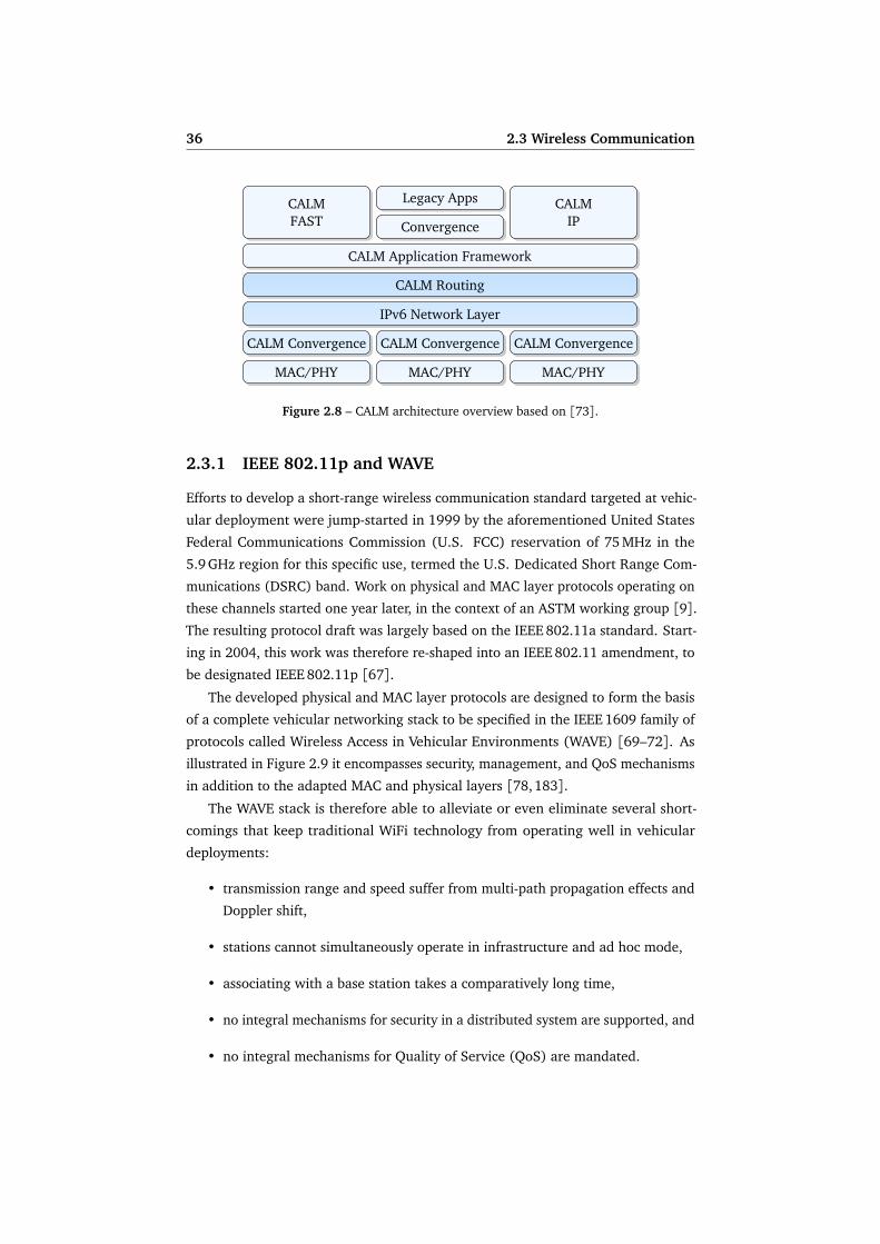
range), which is illustrated in Figure 2.8.
This architecture is envisioned to allow applications to transparently communi-
cate using the best (for varying definitions of best) of any wireless communication
technology that is available to a vehicle at any given moment – as well as to seam-
lessly migrate to different technologies if and when they become available.
Two very different wireless communication technologies constitute two major
pillars of support for the CALM system and are consistently recommended as a basis
for both safety and comfort applications, respectively.
First, the Wireless Access in Vehicular Environments (WAVE) series of standards,
which is based on IEEE 802.11p. Secondly, cellular communication based on, e.g.,
the Universal Mobile Telecommunications System (UMTS). In the following, we
present a brief overview of these candidates, as well as highlight their particular
benefits and drawbacks.
36 2.3 Wireless Communication
IPv6 Network Layer
CALM Routing
CALM Application Framework
CALMFAST
Legacy Apps
Convergence
CALMIP
CALM Convergence
MAC/PHY
CALM Convergence
MAC/PHY
CALM Convergence
MAC/PHY
Figure 2.8 – CALM architecture overview based on [73].
2.3.1 IEEE 802.11p and WAVE
Efforts to develop a short-range wireless communication standard targeted at vehic-
ular deployment were jump-started in 1999 by the aforementioned United States
Federal Communications Commission (U.S. FCC) reservation of 75 MHz in the
5.9 GHz region for this specific use, termed the U.S. Dedicated Short Range Com-
munications (DSRC) band. Work on physical and MAC layer protocols operating on
these channels started one year later, in the context of an ASTM working group [9].The resulting protocol draft was largely based on the IEEE 802.11a standard. Start-
ing in 2004, this work was therefore re-shaped into an IEEE 802.11 amendment, to
be designated IEEE 802.11p [67].
The developed physical and MAC layer protocols are designed to form the basis
of a complete vehicular networking stack to be specified in the IEEE 1609 family of
protocols called Wireless Access in Vehicular Environments (WAVE) [69–72]. As
illustrated in Figure 2.9 it encompasses security, management, and QoS mechanisms
in addition to the adapted MAC and physical layers [78,183].
The WAVE stack is therefore able to alleviate or even eliminate several short-
comings that keep traditional WiFi technology from operating well in vehicular
deployments:
• transmission range and speed suffer from multi-path propagation effects and
Doppler shift,
• stations cannot simultaneously operate in infrastructure and ad hoc mode,
• associating with a base station takes a comparatively long time,
• no integral mechanisms for security in a distributed system are supported, and
• no integral mechanisms for Quality of Service (QoS) are mandated.

2.3 Wireless Communication 37
1609
.380
2.11
p 1609
.41609
.2
Secu
rity
Man
agem
ent
WAVE PHY
WAVE MAC and Channel Coordination
WAVE PHY
TCP / UDP
IPv6WSMP
LLC
Figure 2.9 – Overview of the WAVE stack and associated standards basedon [78,183].
On the physical layer, these issues are addressed by basing IEEE 802.11p on
the Orthogonal Frequency Division Multiplexing (OFDM) mode well-known from
IEEE 802.11a operation, but adapting it to vehicular environments – the main
difference in operation (besides more stringent transmission masks and receiver
performance requirements) being that the channel width is commonly chosen to be
10 MHz instead of the usual 20 MHz, which can easily be accomplished by doubling
all timing parameters [78].
Based on this value, the 75 MHz of the U.S. DSRC band are envisioned to be
used by allocating seven separate 10 MHz channels for data exchange, as illustrated
in Figure 2.10, and similar efforts are underway in Europe and Japan [47].
The center channel is designated the Control Channel (CCH): its use is restricted
to the exchange of control and safety messages. Four channels surrounding the CCH
are designated Service Channels (SCHs): after coordinating their use on the CCH,
stations may transmit on any of these channels to exchange non-safety messages.
Two more channels located at the top and bottom ends of the spectrum remain
reserved for special use.
On the link layer, many of the shortcomings of traditional WiFi technology
are addressed by allowing stations to operate in a special WAVE mode [67]. This
allows any station to address packets to a wildcard Basic Service Set (BSS), causing
receiving stations to process these packets regardless of the BSS with which they
are currently associated.
Similarly, the traditional BSS setup protocol was complemented by stations’
ability to join a WAVE Basic Service Set (WBSS). Other than the process of forming
or joining a regular BSS, forming or joining a WBSS does not entail any data
exchange: this decision is made locally and merely made known to the radio stack’s
lower layers, followed by the optional periodic broadcast of On-Demand Beacons
advertising the WBSS. This also has the side effect of eliminating the traditional
split between hosts and access points.

38 2.3 Wireless Communication
U.S.
Europe
Japan
CCHSCHSCH SCHSCH
5.890 GHz5.880 GHz 5.900 GHz 5.910 GHz5.870 GHz
Figure 2.10 – Spectrum available in the U.S. DSRC band for use as ControlChannel (CCH) and general-purpose Service Channels (SCHs). Below: Cur-rent and future spectrum allocated for ITS use in Europe and Japan; basedon [47,78].
QoS requirements of vehicular networks are met by two mechanisms: first, as
mentioned, a WAVE system employs multiple channels for data transmission, the
use of which is coordinated via beacons on the CCH. As stations are not mandated
to be equipped with multiple transceivers, it needs to be ensured that such beacons
are only sent while all stations are guaranteed to be tuned to the CCH – otherwise
they might miss control or safety messages.
This is achieved by defining CCH intervals: for (by default) any first 50 ms of a
100 ms slot (synchronized via, e.g., the GPS time signal) a station needs to tune to
the CCH to listen for management and safety messages.
As a second mechanism of enforcing QoS, WAVE mandates the use of an En-
hanced Distributed Channel Access (EDCA) mechanism for coordinating channel
access, in a similar fashion to the mechanism described in IEEE 802.11e.
According this mechanism, each regular data transmission will be assigned an
Access Class (AC), influencing its contention window, transmission opportunity limit,
and (most importantly) the Arbitrary Inter-Frame Spacing (AIFS) to delay channel
accesses by, making it more likely that higher-priority services will be able to access
the channel.
Higher-layer additions of WAVE to the traditional IEEE 802.11 stack include the
introduction of the WAVE Short Message Protocol (WSMP) [72], a very lightweight
protocol for the exchange of small single-frame messages geared towards deployment
in WAVE systems, as well as provisions for transmit power management, dynamic
frequency selection, and security [71].
Based on these mechanisms the WAVE stack can provide an integrated solution
to wireless communication requirements of Car-to-X systems that is loosely based
on well-established consumer WiFi technology, albeit only at short ranges. This
means that any system operating purely on a basis of WAVE communication will be
dependent on sufficient penetration rates of either equipped vehicles or supporting
infrastructure.

2.3 Wireless Communication 39
2.3.2 UMTS
A convenient way of avoiding the need for deployment of additional infrastructure
for supporting Car-to-X communication is offered by cellular networks. A suitable
system of cellular networks that is already in widespread use is the Universal Mobile
Telecommunications System (UMTS), a third-generation (3G) mobile telecommuni-
cations technology.
UMTS is being developed and standardized by the Third Generation Partner-
ship Project (3GPP), an organization of telecommunications standards bodies like
the European Telecommunications Standards Institute (ETSI) or the Alliance for
Telecommunications Industry Solutions (ATIS).
Technically, the name UMTS refers to a set of standards, rather than a single
one. To give an example, the UMTS air interface, called Universal Terrestrial
Radio Access (UTRA). This interface can take the form of either a Frequency
Division Duplex (FDD) system for separating mobile station (uplink) and base
station (downlink) traffic and wideband Code Division Multiple Access (CDMA) for
further channelization, or it can employ one of several forms based on Time Division
Duplex (TDD).
As UMTS is an actively evolving system, new features are continuously integrated.
A series of numbered UMTS Releases describes which features are present in a
particular version of UMTS. Examples of such are UMTS Release R99, the first
release of third generation specifications, or UMTS Release Rel-4, which adds –
among other features – the Multimedia Messaging Service (MMS).
UMTS data transmission is based on the concept of transport channels which are
further mapped onto physical channels to be multiplexed to form a data stream. In
the following, we shortly describe three of these channels which are of particular
interest for Car-to-X communication [166].
Dedicated Channel (DCH) Data in a UMTS system will typically be transported
via a DCH, a channel that exists both in the uplink and the downlink. A DCH
needs to be established for each communicating mobile device prior to use
and takes up dedicated resources to guarantee collision freeness.
Correct operation of the CDMA mechanism further requires closed-loop power
control to be performed between mobile equipment and base station: based
on the continuous exchange of management data, mobile devices keep adjust-
ing their transmit power to balance received signal strength and amount of
interference caused.
This means that each DCH requires considerable network resources to be
maintained.
40 2.3 Wireless Communication
Pow
er r
amp
step
P p-m
RACHmessage
Positive Acknowledgementreceived from NodeB
tran
smit
pow
er le
vel
time
Timeout
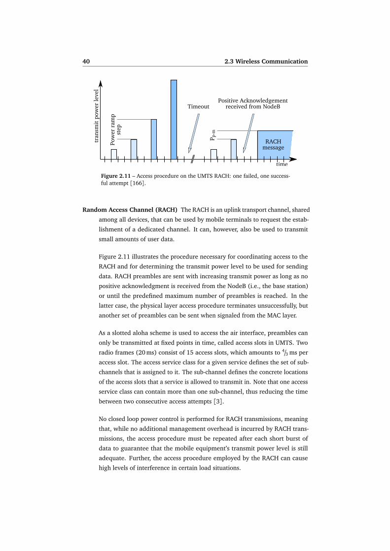
Figure 2.11 – Access procedure on the UMTS RACH: one failed, one success-ful attempt [166].
Random Access Channel (RACH) The RACH is an uplink transport channel, shared
among all devices, that can be used by mobile terminals to request the estab-
lishment of a dedicated channel. It can, however, also be used to transmit
small amounts of user data.
Figure 2.11 illustrates the procedure necessary for coordinating access to the
RACH and for determining the transmit power level to be used for sending
data. RACH preambles are sent with increasing transmit power as long as no
positive acknowledgment is received from the NodeB (i.e., the base station)
or until the predefined maximum number of preambles is reached. In the
latter case, the physical layer access procedure terminates unsuccessfully, but
another set of preambles can be sent when signaled from the MAC layer.
As a slotted aloha scheme is used to access the air interface, preambles can
only be transmitted at fixed points in time, called access slots in UMTS. Two
radio frames (20 ms) consist of 15 access slots, which amounts to 4/3 ms per
access slot. The access service class for a given service defines the set of sub-
channels that is assigned to it. The sub-channel defines the concrete locations
of the access slots that a service is allowed to transmit in. Note that one access
service class can contain more than one sub-channel, thus reducing the time
between two consecutive access attempts [3].
No closed loop power control is performed for RACH transmissions, meaning
that, while no additional management overhead is incurred by RACH trans-
missions, the access procedure must be repeated after each short burst of
data to guarantee that the mobile equipment’s transmit power level is still
adequate. Further, the access procedure employed by the RACH can cause
high levels of interference in certain load situations.

2.3 Wireless Communication 41
Forward Access Channel (FACH) The UMTS Forward Access Channel (FACH) is
a downlink transport channel shared among all devices. Messages that are
sent by the NodeB using the FACH can be received by all mobile stations in a
cell. It can thus be used for multicast transmission of messages, via the UMTS
Multimedia Broadcast Multicast Service (MBMS) mechanism, if supported by
the network.
As the time slots for FACH transmissions are managed by the base station, no
further coordination of channel access needs to take place. However, direct
use of the FACH to reach a single mobile device requires prior knowledge
about the location of the device.
In most densely populated areas (i.e., likely target markets), such UMTS net-
works have already reached sufficient penetration rates for uninterrupted coverage.
Together with the inherent property of cellular networks, the transmission delay
being largely independent from the distance between communicating nodes, this
makes them a salient candidate for transporting Car-to-X communication data from
and to a Traffic Information Center (TIC).
Nonetheless, delays in a cellular network will never be as low as those reachable
in short-range radio communication networks like WAVE [192]. From the descrip-
tion of the mechanisms available in UMTS it is also evident that high data load, in
particular when focusing on low delay, incurs substantial cost in terms of network
resources. Moreover, as the current infrastructure deployment is naturally geared
towards the current target market (i.e., city cores), it is unlikely that this deployment
can easily support as many users trying to concurrently access the system on outlying
highways. Finally, it needs to be noted that multi-operator interoperation issues of
UMTS-based Car-to-X communication systems are still largely unexplored.


2.4 Paradigms and Protocols 43
Car-to-X
Non-Safety Safety
ComfortTraffic Information
SystemsSituation
AwarenessWarningMessages
ContextualInformation
EntertainmentOptimal Speed
Advisory
Congestion,Accident
Information
AdaptiveCruise Control
Blind SpotWarning
Traffic LightViolation
ElectronicBrake Light
Figure 2.12 – Taxonomy of IVC applications.
2.4 Paradigms and Protocols
Based on the presented wireless communication technologies – and coupled with
the availability of affordable hardware powerful enough to support it – a whole
range of possible IVC applications appear to be within reach [194].
In general, this wealth of applications can be distinguished by whether a par-
ticular system is geared towards keeping drivers informed and/or entertained or
towards directly increasing the safety of drivers [195], as illustrated in Figure 2.12.
Safety applications (e.g., systems supporting situation awareness or disseminat-
ing warning messages), will typically need to send comparatively few and small
messages, but those need to be delivered under very strict latency and reliability
constraints.
Non-Safety applications (e.g., comfort applications and traffic information sys-
tems), on the other hand, typically deal with much larger data volumes, albeit under
comparatively lenient latency and reliability constraints.
As a general trend, this divide between safety and non-safety related applications
can be seen reflected in a divide between single hop and multi hop applications.
Single hop wireless communication protocols are focusing more on safety applica-
tions [105], while multihop protocols still dominate in the areas of traffic congestion
avoidance and dedicated information systems [198]. Further, with the advent of
3G+ communication systems, comfort applications can easily be realized using
direct one-to-one connections between a vehicle and a base station. Thus, in the
following, we focus on distributed Traffic Information System (TIS) applications,
where system-level challenges like efficient multi-hop operation and scalability as
well as disconnected operation are still very prevalent.

44 2.4 Paradigms and Protocols
In this domain, a huge number of protocols have been proposed in the last
decade and this trend is continuing. In the following, we therefore give a brief
overview over current approaches by presenting examples based on three very
different paradigms: ad hoc routing (Section 2.4.1), flooding (Section 2.4.2), and
beaconing (Section 2.4.3).
2.4.1 Ad Hoc Routing: The DYMO Protocol
Numerous approaches to information dissemination in Car-to-X communication
systems have applied MANET routing techniques for establishing a Vehicular Ad Hoc
Network (VANET) in its strongest sense, i.e., they applied ideas from MANET re-
search for establishing networks of vehicles [118,147,188]. For the provision of TIS
services, such ad hoc networks can then be connected (via dedicated infrastructure)
to a TIC or to the Internet.
Research on MANETs addresses a wide range of objectives [114,132]; thus, a
wide range of protocols have been proposed in the last decade [6,65,74]. In general,
these routing protocols can be differentiated according to their method of acquiring
and distributing routing information [40].
Three basic classes are commonly identified: proactive, reactive, and hybrid
protocols [114]. The basic characteristics of these classes are described in the
following.
Proactive routing protocols rely on the periodic exchange of topology information.
All such protocols essentially always maintain up-to-date routing information,
which can then be used to forward data packets through the network towards
their destination. Depending on the specific protocol and the degree of
mobility, periodic routing updates can require a remarkable amount of network
overhead for state (topology) maintenance.
The best known example of a table-driven ad hoc routing protocol is the
Destination Sequenced Distance Vector (DSDV) protocol [127].
Reactive routing protocols have been introduced to prevent the periodic exchange
of routing information, which may consume an essential amount of the avail-
able network resources. The core idea of reactive routing is to only search for
paths through the network if data packets need to be transmitted.
The first protocol of this class was developed back in 1994: the Dynamic
Source Routing (DSR) protocol [79]. One of the more current approaches
and probably the one best known in the ad hoc networking community is the
Ad Hoc on Demand Distance Vector (AODV) protocol [128].

2.4 Paradigms and Protocols 45
Hybrid routing protocols try to exploit the specific advantages of proactive routing
protocols (i.e., fast delivery of packets as routing information is always avail-
able) and reactive routing protocols (i.e., reduced cost in terms of network
overhead for state maintenance).
A typical example is the Zone Routing Protocol (ZRP) [62]. ZRP distinguishes
between a local neighborhood called the routing zone, for which routing
information is maintained proactively, and all destinations beyond the routing
zone, for which routes are acquired on demand.
Standardization of MANET routing protocols is the focus of the Internet En-
gineering Task Force (IETF) MANET working group, which aims to propose one
candidate protocol each from the domains of proactive and reactive routing based on
a Generalized MANET Packet/Message Format [30]. When considering applications
in VANET scenarios that require multi-hop communication, delay appears to be
less of an issue compared to the overhead of maintaining full topology information
under high mobility. Thus, we are focusing on the MANET working group’s reactive
routing protocol candidate, called Dynamic MANET On Demand (DYMO) [24].As the working group is chartered to re-use mature components from previous
work on experimental protocols, DYMO builds heavily upon experience with previous
approaches to reactive routing, especially with the routing protocol AODV.
DYMO is able to set up and maintain unicast routes in IPv4 and IPv6 network
scenarios by using the following mechanism:
1. In order to discover a new route to a peer, a node transmits a Route Request
(RREQ) to all nodes in range. This can be achieved by sending the message to
a designated link-local multicast address that is associated with all MANET
routers. When an intermediate node receives such an RREQ, it takes note of
previously appended information, deducing routes to all nodes the message
previously passed through. The node then appends information about itself
and passes the message on to all nearby nodes. This way, the RREQ is
effectively flooded through the MANET and, after a potentially large number
of hops, eventually reaches its destination.
2. The destination responds to the received RREQ by sending a Route Reply
(RREP) via unicast back to the last hop it received the RREQ from. As with
the propagation of an RREQ, this node again appends information about itself
and takes note of all routing information contained in the RREP. With the
help of the routing information previously obtained while forwarding the
corresponding RREQ, the intermediate node is able to send the RREP further
back to the start of the chain, until it eventually reaches the originating node.
This node will now know a route to the requested destination, as well as
routes to all intermediate nodes, and vice versa.

46 2.4 Paradigms and Protocols
DYMO:
a
a,ba,b,c
d,c,b
d,cd
A
BC
DAODV:
a
aa
d
dd
A
BC
D
Figure 2.13 – Routing information dissemination in AODV and DYMO.
DYMO retains proven mechanisms of previously explored routing protocols like
the use of sequence numbers to enforce loop freedom or allowing intermediate
nodes to generate RREPs on behalf of an RREQ’s destination if a suitable route
was already stored. However, it aims at a somewhat simpler design, helping to
lower the nodes’ system requirements and simplify the protocol implementation.
At the same time, DYMO provides enhanced features, such as natively supporting
MANET-Internet gatewaying and implementing path accumulation as follows.
Besides route information about a requested target, a node will also receive
information about all intermediate nodes of a newly discovered path. Therein lies a
major difference between both protocols: AODV only generates route table entries
for the destination node and the next hop node, while DYMO stores routes for each
intermediate hop. This is illustrated in Figure 2.13. When using AODV, node A
knows only the routes to B and D after the route request is satisfied. In DYMO, the
node additionally knows a route to node C.
To efficiently deal with highly dynamic scenarios, links on known routes may
be actively monitored, e.g., by using the MANET Neighborhood Discovery Protocol
(NHDP) [29] or by examining feedback obtained from the data link layer. An
implementation may also choose to not actively monitor links, but instead to simply
drop inactive routes. Detected link failures are made known to the MANET by
sending an RERR to all nodes in range, informing them of all routes that now
became unavailable. Should this Route Error (RERR) in turn invalidate any routes
known to these nodes, they will again inform all their neighbors by multicasting an
RERR containing the routes concerned, thus effectively flooding information about
a link failure through the MANET.
DYMO is thus a salient candidate for lightweight topology maintenance in mobile
networks, performing routing tasks to support message exchange. However, while
multipath extensions have been designed and investigated in order to improve the
throughput in MANETs [53], by its nature, DYMO is not geared towards wide-area
message dissemination, but rather towards maintaining point to point connectivity.

2.4 Paradigms and Protocols 47
idlestart sendrcv
dup
Figure 2.14 – Concept of a simple flooding scheme for information dissemina-tion in MANETs.
0 20 40 60 80 100
05
10
15
20
25
30
01
02
03
04
05
06
0
node density in nodes/km
del
ay i
n m
s
pac
ket
lo
ss r
atio
in
%
total delaymac delaypkt loss
Figure 2.15 – Impact of the broadcast storm problem on network performance;based on results presented in a study of flooding on a 10 km four lane highwayreported in [177].
2.4.2 Flooding: The DV-CAST Protocol
Flooding of data, also known as multi-hop broadcast, addresses the topic of wide-
area message dissemination in mobile networks. A very simple and straightforward
mechanism that works in a similar fashion to the flooding of RREQ packets in DYMO
is illustrated in Figure 2.14. When a node receives a packet for the first time (labeled
rcv in the figure), it is immediately re-broadcast. When a node receives a duplicate
packet (labeled dup), the packet is consumed without any action.
However, this mechanism ensures little more than that the broadcast will eventu-
ally die out. In particular, this flooding technique broadcasts that many more packets
than would be required to ensure 100 % dissemination that its effects are commonly
termed a broadcast storm [89,119,177]. Because these superfluous transmissions
all compete with each other and with unrelated data transmissions, packet delay,
access delay, and packet loss rise sharply – both for the flooding application and for
other applications in the network (cf. Figure 2.15). More sophisticated approaches
to flooding thus implement additional measures to not re-broadcast every packet
received, but to selectively suppress broadcasts.
One such mechanism is based on a simple estimation of the distance between
current node i and message sender j, i.e., it does not require the exchange of
neighborhood information or the maintenance of topology [199].

48 2.4 Paradigms and Protocols
idlestart wait Ti j send
wait δ′
rcv
dup
p
¬p
expired
dup
Figure 2.16 – Concept of a family of distance based schemes for broadcastsuppression.
This distance is expressed as 0 ≤ %i j ≤ 1, i.e., in relation to a maximum distance
between nodes. Among the approaches that can be used for estimating %i j are calcu-
lations based on the calculated distance Di j to the GPS position of the sending node
or on the measured Received Signal Strength (RSS) value of a received transmission,
e.g., in the fashion outlined in Equations (2.3) and (2.4), respectively.
%i j =
⎧⎪⎪⎪⎪⎪⎨⎪⎪⎪⎪⎪⎩
0 if Di j < 0Di j
R if 0 ≤ Di j < R (approx. transmission radius)
1 otherwise
(2.3)
%i j =
⎧⎪⎪⎪⎪⎪⎨⎪⎪⎪⎪⎪⎩
0 if RSSx < RSSminRSSmax−RSSx
RSSmax−RSSminif RSSmin ≤ RSSx < RSSmax
1 otherwise
(2.4)
Based on either of these metrics, the following approach (illustrated in Fig-
ure 2.16) is used. When receiving a packet for the first time, a node will first wait
for a short interval Ti j . After this interval has elapsed, it will then re-broadcast
the packet, but only with a certain probability p. In the event that it chooses not
to re-broadcast the packet, it will wait an additional interval δ′ (chosen so that
∀Ti j ∶δ′ > Ti j) to check that it overhears at least one re-broadcast by another node,
thus preventing message die-out. This approach could thus be categorized as broad-
cast suppression based on waiting and overhearing; in addition it favors larger per
hop distances over smaller ones.
Three different schemes for choosing Ti j and p are given in [199]. Weighted
p-persistence uses a pre-configured value Ti j and chooses p = min{%i j} based on
all duplicates received during waiting. Slotted p-persistence and slotted 1-persistence
use a fixed forwarding probability p (or p = 1, respectively) and choose Ti j =τ × ⌈Ns (1 − %i j)⌉ based on a configured time step τ and number of slots Ns.

2.4 Paradigms and Protocols 49
All flooding schemes, however, have one common weakness: if parts of the
network are temporarily disconnected, pure flooding approaches will never be able
to reach them.
Therefore, the concept of flooding has been combined with Delay/Disruption
Tolerant Network (DTN) approaches to form hybrid flooding schemes. The most
recent of such advanced schemes, which perform flooding in well-connected net-
works and perform store-carry-forward when the network is disconnected, is called
DV-CAST [179].
To achieve the desired effect, DV-CAST mandates that nodes periodically broad-
cast short Hello beacons containing GPS information. Each node then stores infor-
mation on received Hello beacons in three distinct tables: one table stores neighbors
driving in the same direction and in front of the current node, one stores neighbors
driving in the same direction and behind the current node, and one table stores
neighbors driving in the opposite direction.
Based on theses tables, a node can then decide for each received message
whether it is more beneficial to perform flooding, or whether the message needs to
be buffered before it can be re-broadcast. DV-CAST also handles the special case of
what the authors call a sparsely connected network, i.e., one where only nodes on
the opposite lane can be reached. In these cases, it can exert further control about
handing off responsibility between the opposing and the same lane.
In order to achieve this functionality, the following algorithm is applied for
relaying a message:
Totally disconnected conditions are assumed if no neighbor can be found driving
in either direction. In this case store-carry-forward is performed until new
neighbors can be found driving in either direction.
Sparsely connected conditions are assumed if only a neighbor driving in the op-
posite direction can be found. In this case responsibility for the message is
immediately transferred to this neighbor, which will then have to ensure either
the delivery of the message to its destination or back to a vehicle driving in
the original direction.
Well connected conditions are assumed if a neighbor can be found driving in the
same direction behind the current node and the message is supposed to be
forwarded to the back, or vice versa. In this case broadcast suppression
according to one of the described algorithms is performed.
This means that, although DV-CAST will temporarily buffer some messages, it
will never permanently store any information, thus focusing more on the exchange of
short-lived events, where message dissemination is likely to be a one shot operation.

50 2.4 Paradigms and Protocols
t = t0
t = t1
t = t2
Figure 2.17 – Message dissemination via beaconing, as envisioned in SOTIS.
2.4.3 Beaconing: The SOTIS Protocol
Other than the aforementioned protocols, the Self-Organizing Traffic Information
System (SOTIS) [197] is designed for the dissemination of information (pertaining,
e.g., to current traffic conditions), rather than atomic events.
This is accomplished by each car keeping a local knowledge base which inte-
grates both locally-generated sensor data and data received from other participating
cars. Cars will then periodically send a broadcast packet that contains part of the
local knowledge base, termed a beacon. This way, knowledge (about, e.g., road
conditions) will be gradually disseminated among participating cars, even if the
network sporadically becomes disconnected, as illustrated in Figure 2.17: as even
isolated clusters of cars will infrequently receive beacons transmitted, e.g, by ve-
hicles driving in the opposite lane, information dissemination is not stopped, but
merely slowed down in these cases. Based on the accumulated contents of their
local knowledge bases, cars will still be able to perform road traffic analysis or warn
the user about oncoming hazards.
As the default beacon interval is envisioned to be on the order of seconds (the
authors give 5 s as an example), there exists a separate mechanism that is able to
transmit emergency messages for immediate transmission (and re-integration into
the knowledge bases of receiving cars). For this, it is assumed that the MAC layer
protocol guarantees immediate access to the channel, e.g., by always reserving some
capacity for emergency reports.
In order to conserve network resources, each car stores and transmits information
pertaining not to specific points, but to small segments of roads. Each car determines
the length of a segment (and, thus, the granularity of information) dependent on
its distance to the segment. As cars are envisioned to be equipped with compatible

2.4 Paradigms and Protocols 51
α3
2
1
Figure 2.18 – On-the-fly generation of road maps for SOTIS.
digital maps, they are able to assign a unique identifier to each road. Together with
segment based addressing, this road identifier allows for a space efficient encoding.
If (compatible) maps cannot be assumed to be available in each participating car,
the authors later proposed an extension [196] to SOTIS, which was evaluated [45]and adapted for use in the ongoing simTD [174] project. This extension enables cars
to generate road maps on the fly based on GPS information, as well as to exchange
information about them in a highly efficient manner via Car-to-X communication.
This process is based on a reference grid of virtual lines spaced Dgrid apart, as
illustrated in Figure 2.18. Each time a vehicle crosses a grid line (cf. ¬ in the
figure), it generates a Geo-Reference Point at the location of intersection. In order
to ward against the case of creating spurious points caused by positioning errors,
no point is created when crossing a line at an angle smaller than a pre-configured
α (cf. ® in the figure). In a second step, sequences of points are assembled into
one Geo-Reference List each; based on these lists an approximate digital map can
be derived and exchanged between cars. Creating and storing duplicate points is
warded against based on a simple distance metric: if a new point is closer than a pre-
configured position inaccuracy Dacc to an existing one (and the associated list runs in
a compatible direction), the new point is assumed to be referring to the same point
and the existing one is used instead. While this process cannot guarantee matching
map data if positioning errors are unexpectedly high or lanes are unexpectedly wide
(cf. in the figure), it comes reasonably close: in a simulation experiment [196]authors claimed a mean deviation of generated map data by approximately half the
Root Mean Square Error (RMSE) in position estimation.
A Car-to-X communication system based on this (extended) SOTIS approach is
thus able to operate without deployment of infrastructure on the road and without
digital maps on the vehicles (much less the deployment of identical ones). Informa-
tion can be shared using a highly efficient data encoding based on road segments
and no information is lost during sporadic network disconnections.

52 2.4 Paradigms and Protocols
This makes SOTIS a salient candidate for information dissemination with multi-
ple possible avenues for future improvements:
Incorporation of infrastructure: Information dissemination becomes noticeably
slower when market penetration of the system is still low, as the authors re-
mark. An approach that could incorporate available infrastructure in addition
to being able to operate in a completely infrastructure-less fashion would help
bridge this gap.
Adaptivity to scenarios: The authors of SOTIS note that it might be favorable to
determine the beacon interval in an adaptive fashion, rather than using a fixed
schedule for the dissemination of information. An approach that could take
into account indications of past, present, and future channel use, as well as
the usefulness of information to the network as a whole, would help achieve
the fastest possible dissemination rates without ever overloading the channel.
Medium sharing: The MAC layer access protocol that SOTIS is deployed on is
required to be able to guarantee immediate access to the channel, so that the
medium can be shared between both comfort oriented and safety relevant
messages. It is noted that this can easily be achieved by always reserving some
capacity for emergency reports, yet this static allocation means that a substan-
tial portion of channel capacity is wasted. An approach that could incorporate
safety relevant messages to be transmitted over the same protocol, as well as
coexist with other and future protocols would allow for a more efficient use of
the channel capacity, while making sure that low delay transmission of safety
messages can be achieved.
We address these questions in Chapter 4 and demonstrate how to fill this gap
without sacrificing scalability or performance, both in purely ad hoc scenarios and in
infrastructure-assisted settings. Before we do so, however, we introduce in Chapter 3
our methodology for assessing such metrics of Car-to-X communication systems.

Chapter 3
Simulating Car-to-X Communications
3.1 The Veins Simulation Framework . . . . . . . . . . . . . . . . . . . . . 57
3.1.1 Design Principles . . . . . . . . . . . . . . . . . . . . . . . . . . 58
3.1.2 Parameter Studies and Simulation Control . . . . . . . . . . . 64
3.2 Performance Metrics . . . . . . . . . . . . . . . . . . . . . . . . . . . . 67
3.2.1 Estimating the Environmental Impact . . . . . . . . . . . . . . 68
3.2.2 Simulation Model and Setup . . . . . . . . . . . . . . . . . . . 69
3.2.3 Comparison of Selected Metrics . . . . . . . . . . . . . . . . . 70
3.2.4 Conclusion . . . . . . . . . . . . . . . . . . . . . . . . . . . . . . 73
3.3 Signal Propagation and Shadowing . . . . . . . . . . . . . . . . . . . . 75
3.3.1 Related Work on Signal Propagation and Shadowing . . . . . 77
3.3.2 Data Basis and Measurements . . . . . . . . . . . . . . . . . . 78
3.3.3 A Computationally Inexpensive Obstacle Model . . . . . . . . 81
3.3.4 Comparison of Model and Measurements . . . . . . . . . . . . 83
3.3.5 Conclusion . . . . . . . . . . . . . . . . . . . . . . . . . . . . . . 85
3.4 Road Networks . . . . . . . . . . . . . . . . . . . . . . . . . . . . . . . 87
3.4.1 Using OpenStreetMap Data in Veins . . . . . . . . . . . . . . . 87
3.4.2 Comparison of Results Dependent on Geodata Quality . . . . 90
3.4.3 Conclusion . . . . . . . . . . . . . . . . . . . . . . . . . . . . . . 92
3.5 The Impact of Car-to-X Communication . . . . . . . . . . . . . . . . . 93
3.5.1 Impact on Travel Time . . . . . . . . . . . . . . . . . . . . . . . 94
3.5.2 Impact on Emissions . . . . . . . . . . . . . . . . . . . . . . . . 95
3.5.3 Impact on Road Network . . . . . . . . . . . . . . . . . . . . . 98
3.5.4 Impact on Route Choice . . . . . . . . . . . . . . . . . . . . . . 98
3.6 Conclusion . . . . . . . . . . . . . . . . . . . . . . . . . . . . . . . . . . 103
53


3 Simulating Car-to-X Communications 55
In the previous chapter we explained why performance evaluation of Car-to-X
communication protocols, such as wireless communication, multihop routing, and
application-aided broadcast, is typically performed in network simulation environ-
ments. We also showed how the mobility models that are integrated in common
network simulation frameworks are inadequate for the performance evaluation of
Car-to-X communication systems because of their low degree of realism. We further
demonstrated how movement trace data, generated using road traffic simulation
frameworks which implement well-established vehicular mobility models, can be
used to accurately model the movement of real cars in simulations.
However, in cases where, e.g., accident information, hazard warnings, or road
congestion information are exchanged between vehicles – and where this informa-
tion can be assumed to influence drivers’ behavior – the reliance on trace data fails
to capture realistic node movement: the major drawback of off-line mobility traces,
both pre-generated ones and those obtained from real-world measurements, is that
they can only model the influence of road traffic on network traffic, but not vice
versa.
In this chapter, parts of which are based on our articles published in IEEE Trans-
actions on Mobile Computing [162], IEEE Communications Magazine [156], and
GI Praxis der Informationsverarbeitung und Kommunikation [157], as well as pre-
sented at conferences and workshops [42,151,154,159,164,169,170], we demon-
strate how we helped bridge this gap and take simulative evaluation of Car-to-X
communication systems one step further. We describe the observations that led us to
the creation of our Veins simulation framework as well as its underlying components
which we consider prerequisites for accurate performance evaluation of Car-to-X
communication protocols.


3.1 The Veins Simulation Framework 57
Network Simulation Road Traffic Simulation
D. bidirect.coupling
C. micro-simulation
B. recordedtraces
A. integratedmodels
Figure 3.1 – Mobility modeling techniques for simulation of IVC protocolsand applications.
3.1 The Veins Simulation Framework
Whenever events in a network simulation can potentially affect the mobility of
vehicles, any approach based on trace data is unable to generate the required real-
time interaction between mobility model and application model. For example, in
vehicular safety applications, vehicles will generate alert messages to change the
mobility patterns of other vehicles. Thus, the vehicles can be expected to change
their speed or route according to the received information. In this case, the network
simulation model and the mobility simulation model need to interact with each
other in a real-time manner.
While there exist approaches, such as the NCTUns simulation environment [189],which allow integrated network and traffic simulation, those are often developed
from scratch. Thus, the employed models of network and road traffic microsimu-
lation are hard to validate against and compare with the manifold well-tested and
proven models by experts from the respective fields available in common network
and road traffic simulation frameworks.
It was therefore deemed beneficial to instead base simulations on a bidirec-
tionally-coupled simulation environment that unifies existing frameworks from the
network simulation and the road traffic simulation domains. Compared to ap-
proaches relying on generated trace data, the only drawback of such a simulator is
that the results of the road traffic simulation cannot be re-used in the form of trace
files, as in bidirectionally coupled simulations node mobility is typically influenced
by network communication and, thus, has to be computed on-the-fly.
Figure 3.1 gives an architectural view of the presented mobility modeling tech-
niques for Inter-Vehicle Communication (IVC) simulation. While random node
movement is usually an integrated component of state-of-the-art network simulation
tools, traces can only be obtained by external processes; either by collecting move-
ment data in real world experiments, or by means of road traffic microsimulation
tools. Finally, bidirectionally coupled simulation relies on intensive intercommunica-
tion of the different simulation tools using appropriate interfaces.

58 3.1 The Veins Simulation Framework
Building upon this and the conclusions drawn in Section 2.2, the benefits and
drawbacks of different mobility modeling approaches can be summarized as follows:
Random Movement
⊞ Straightforward, intuitive
⊞ Readily available
⊟ Unrealistic topology dynamics
⊟ Potentially unstable
Real-World Traces
⊞ Most realistic node movement
⊞ Re-usable traces
⊟ Costly and time-consuming to generate
⊟ No free parameterization
Artificial Mobility Traces
⊞ Realistic node movement
⊞ Free parameterization
⊞ Re-usable traces
⊟ No feedback on driver behavior
Bidirectionally Coupled Simulators
⊞ Realistic node movement
⊞ Free parameterization
⊞ Feedback on driver behavior
⊟ No re-usable traces
This closely resembles the historical progression of common approaches to
mobility modeling in IVC simulations: early work relied on relatively simple models
using random node movement. Because such mobility models do not realistically
reflect car movement on roads, more complex solutions have been developed based
on real-world and artificial traces of car movement, leading to recent advances
based on tightly coupled road traffic microsimulation and network simulation. In
the following, we present our solution which follows exactly this approach.
3.1.1 Design Principles
We developed Veins (short for Vehicles in Network Simulation) to fill the need for
a simulation framework that incorporates all of the benefits from using mature
and well-established simulators of both the network simulation and the road traffic
microsimulation domains.
Further, the source code of both frameworks needed to be publicly available, so
that simulation results can easily be reproduced by interested researchers.

3.1 The Veins Simulation Framework 59
Figure 3.2 – State machines of network and road traffic simulation frame-works’ coupling modules.
Serving as the basis of Veins are therefore the network simulation core and
associated modules of OMNeT++, as well as the road traffic simulator Simula-
tion of Urban Mobility (SUMO), the advantages of which have been outlined in
Sections 2.1.1 and 2.2.3, respectively.
We achieved bidirectional coupling of both frameworks by extending each with
a dedicated communication module. During simulation runs, these communication
modules exchange commands, as well as mobility data, via a TCP connection.
OMNeT++ is an event-based simulator, so it handles mobility by scheduling
node movements at regular intervals. This fits well with the approach of SUMO,
which also advances simulation time in discrete steps. As can be seen in Figure 3.2,
the control modules integrated with OMNeT++ and SUMO were able to buffer any
commands arriving in-between the simulators’ time steps to guarantee synchronous
execution at defined intervals. At each time step, OMNeT++ would then send
all buffered commands to SUMO and trigger the corresponding time step of the
road traffic simulation. Upon completion of the road traffic simulation time step,
SUMO would send a series of commands and the position of all instantiated vehicles
back to OMNeT++. This allows the network simulation to react to the received
mobility data by introducing new nodes, deleting nodes that had reached their
destination, and moving nodes according to their road traffic simulation counterpart.
After processing all received commands and moving all nodes according to the
mobility information, OMNeT++ would then advance the simulation until the next
scheduled time step, allowing nodes to react to altered environmental conditions
and, thus, a Car-to-X communication system to influence node mobility.

60 3.1 The Veins Simulation Framework
Message Exchange
SUMOOMNeT++/INET
1: SIM_NODE_STOP
2: SIM_NODE_REROUTE
3: SIM_NODE_RESUME
4: SIM_STEP
Se
nd
Co
mm
an
ds
Trig
ger
SU
MO
Tim
est
ep
Ad
van
ce
Sim
ula
tio
n
5: Trace Data
Bu
ffe
r C
om
ma
nd
s
Figure 3.3 – Sequence diagram of messages exchanged between network androad traffic simulation frameworks’ coupling modules. Command execution isdelayed until the next road traffic simulation time step is triggered.
Figure 3.3 shows the interaction between both simulators in the form of a
message sequence chart. Using a simple request/response protocol, road traffic in
SUMO can be influenced by OMNeT++ in a number of ways. Most importantly,
time steps are generated to advance the simulation in SUMO. Furthermore, vehicles
can be stopped to create artificial traffic jams, they can be resumed to resolve those
jams, and each simulated vehicle can be individually rerouted around arbitrary road
segments. This way, Veins accurately reflects how drivers who know about a traffic
obstruction will try to avoid it. More recently, commands have been included to
model vehicles slowing down (e.g., in front of hazards), as well as commands that
allow vehicles and network components to interact with traffic lights.
Thus, two inter-dependent processes are running concurrently, namely the net-
work simulator and the road traffic simulator. Both processes share data like position
and speed of simulated vehicles, while other data like radio state and planned route
is local to the network simulator or the road traffic simulator, respectively. Movement
information updates about simulated vehicles are exchanged at regular intervals.
This results in two alternating phases during bidirectionally-coupled simulation:
1. While the network simulation is running, it sends parameter changes to the
road traffic simulation, e.g., altering driver behavior and influencing vehicles’
routing decisions. Simulation time advances only in the network simulator.
2. At regular intervals, the road traffic simulation performs traffic computations
based on these new parameters and sends vehicle movement updates to
the network simulation. Simulation time advances only in the road traffic
simulator.

3.1 The Veins Simulation Framework 61
1 tsp 02 add host [0000] Car;i= car0_vs ;r=0 , ,#707070 ,13 mov host [0000] 998.35 4995.00 0.00 09014 tsp 85 add host [0001] Car;i= car1_vs ;r=0 , ,#707070 ,16 mov host [0001] 998.35 4976.32 6.74 09017 mov host [0000] 998.35 4943.28 9.83 09018 [...]9 tsp 529
10 del host [0000]11 mov host [0003] 3786.65 998.35 13.89 040412 mov host [0002] 3911.91 998.35 13.90 040413 mov host [0001] 3954.35 998.35 13.89 0404
Listing 3.1 – Excerpt of mobility data sent by an early version of the coupling
interface to the road traffic simulator.
These phases are also evident from Figure 3.3: in the first phase, commands are
sent to SUMO, in the second phase their execution is triggered and the resulting
mobility data received. This way, both simulators are tightly coupled and SUMO
is only able to perform a simulation step after all events within a time step have
been processed in the network simulation. The network simulator advances the
road traffic microsimulation only at fixed intervals.
This means that these intervals need to be sufficiently fine grained to obtain
realistic results: as the network topology will typically never change in between two
time steps in the mobility simulation, care must be taken to execute time steps at
least as frequently as the network simulation can be expected to react to topology
changes. From a performance point of view, this is not a problem because (when
using a high performance road traffic simulation framework such as SUMO) the
time spent for the computation of node mobility is negligible compared to that spent
for the simulation of wireless networks.
Listing 3.1 shows a small sample of the command and mobility data stream
used by an early version of the coupling interface to SUMO [202]. To guarantee
synchronicity of both simulators, each time step is signaled by one tsp command
containing the current simulation time. Using the add command, the road traffic
simulation is able to introduce new vehicles entering the road traffic simulation,
to be represented by an arbitrary OMNeT++ module. Similarly, the road traffic
simulation is able to remove from the network simulation all vehicles that have
reached their destination by issuing del commands. Mobility data is communicated
by transmitting the current speed and position of all instantiated nodes as a series
of mov commands, the position being expressed as both OMNeT++ simulation
coordinates and SUMO lane identifier.
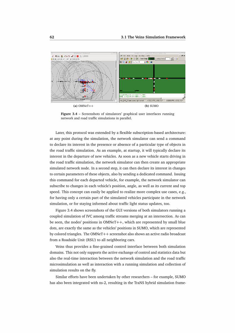
62 3.1 The Veins Simulation Framework
(a) OMNeT++ (b) SUMO
Figure 3.4 – Screenshots of simulators’ graphical user interfaces runningnetwork and road traffic simulations in parallel.
Later, this protocol was extended by a flexible subscription-based architecture:
at any point during the simulation, the network simulator can send a command
to declare its interest in the presence or absence of a particular type of objects in
the road traffic simulation. As an example, at startup, it will typically declare its
interest in the departure of new vehicles. As soon as a new vehicle starts driving in
the road traffic simulation, the network simulator can then create an appropriate
simulated network node. In a second step, it can then declare its interest in changes
to certain parameters of these objects, also by sending a dedicated command. Issuing
this command for each departed vehicle, for example, the network simulator can
subscribe to changes in each vehicle’s position, angle, as well as its current and top
speed. This concept can easily be applied to realize more complex use cases, e.g.,
for having only a certain part of the simulated vehicles participate in the network
simulation, or for staying informed about traffic light status updates, too.
Figure 3.4 shows screenshots of the GUI versions of both simulators running a
coupled simulation of IVC among traffic streams merging at an intersection. As can
be seen, the nodes’ positions in OMNeT++, which are represented by small blue
dots, are exactly the same as the vehicles’ positions in SUMO, which are represented
by colored triangles. The OMNeT++ screenshot also shows an active radio broadcast
from a Roadside Unit (RSU) to all neighboring cars.
Veins thus provides a fine-grained control interface between both simulation
domains. This not only supports the active exchange of control and statistics data but
also the real-time interaction between the network simulation and the road traffic
microsimulation as well as interaction with a running simulation and collection of
simulation results on the fly.
Similar efforts have been undertaken by other researchers – for example, SUMO
has also been integrated with ns-2, resulting in the TraNS hybrid simulation frame-

3.1 The Veins Simulation Framework 63
Figure 3.5 – Screenshot of the running simulative prototype. A contiguousstream of vehicles, leaving the campus and heading to a business park, isinterrupted by a traffic obstruction at point ¬. Dynamic re-routing has started.
work [130] – so more recent efforts aim at establishing a common interface for
coupling any road traffic microsimulation with network simulations. The presented
approach has therefore been integrated together with other approaches into a
generalized traffic control interface, TraCI [190], which is based on the same com-
mand-response approach. Using TraCI, clients of a road traffic simulation can rely
on the same, flexible subscription-based system to receive information about events
in the mobility model and on an event-triggered system for sending commands to
the running mobility simulation. Aside from its use in Veins and TraNS there are
ongoing implementation efforts to integrate this interface for the coupling of the
SUMO and AnSim mobility simulators with the network simulation toolkits Shawn
and JiST/SWANS.
Because of the flexibility afforded by the presented approach, Veins can be
further extended to support communication models based on UML [37, 154] or
external hardware for influencing the simulation. As an example we demonstrated
the impact of a dynamic vehicle re-routing mechanism that is based on real-time
traffic [161]. Here, traffic flows could be controlled and traffic obstructions could
be introduced interactively, making it possible to study both the positive and the
negative effects of a specific Traffic Information System (TIS) on road traffic (a
screenshot of this simulation is reproduced in Figure 3.5). Thus, while Veins still
affords the static evaluation of protocols with respect to almost all common metrics,
it also allows researchers to intuitively grasp their benefits and shortcomings by
interacting in real time with the protocols under consideration.

64 3.1 The Veins Simulation Framework
3.1.2 Parameter Studies and Simulation Control
A straightforward way of performing bidirectionally coupled simulations using Veins
is to first start a road traffic simulation in SUMO, waiting for a TraCI client to
connect. In a second step, after SUMO has started, the OMNeT++ simulation can
be launched, which will then be able to connect to the running SUMO simulator.
However, performance studies of Car-to-X protocols will routinely involve pa-
rameter studies using several runs. Moreover, for a simulation to yield meaningful
results, a single simulation run has to be repeated several times using independent
random numbers for each replication [124].
Finally, to gain confidence that the implemented simulation program does indeed
represent the system which was intended to be modeled with sufficient accuracy,
the simulation has to be validated. In the vast majority of cases, a proof that the
simulation model works as intended is too costly to acquire. Instead, evaluations
and tests are performed to increase the confidence in the model’s correctness. These
evaluations should be continued until a sufficient level of confidence has been
achieved.
Several validation methods have been discussed in the literature (see, for exam-
ple, [141]). In the following, we list some of the methods which are particularly
relevant to simulation models of network protocols [153].
Animation of a simulation yields invaluable information about protocol behavior
on a microscopic level, such as message contents, sources, destinations, and
protocol states.
It is, however, not a substitute for examining the macroscopic behavior via,
e.g., statistical analysis of results [96].
Testing extreme conditions and degenerate cases like jammed conditions on the
road and on the medium, or misbehaving devices, routinely reveals flaws in
the model.
Face validity can be ensured by asking system experts whether the model itself, its
execution, and/or its output behavior seems reasonable.
Operational graphics display the values of performance measures in a time series
(either during or after a simulation run). This can be used to find leads for
further investigations of model behavior or to evaluate the suitability of output
metrics.
Parameter variability and sensitivity analysis consists of systematically varying
the simulation’s input parameters and analyzing how the output reacts to the
variations.
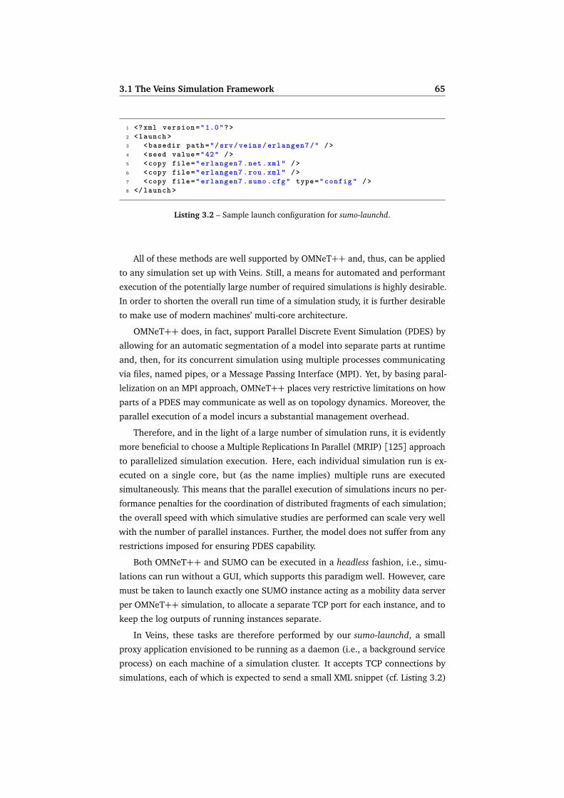
3.1 The Veins Simulation Framework 65
1 <?xml version ="1.0"?>2 <launch >3 <basedir path="/srv/veins/ erlangen7 /" />4 <seed value="42" />5 <copy file=" erlangen7 .net.xml" />6 <copy file=" erlangen7 .rou.xml" />7 <copy file=" erlangen7 .sumo.cfg" type=" config " />8 </ launch >
Listing 3.2 – Sample launch configuration for sumo-launchd.
All of these methods are well supported by OMNeT++ and, thus, can be applied
to any simulation set up with Veins. Still, a means for automated and performant
execution of the potentially large number of required simulations is highly desirable.
In order to shorten the overall run time of a simulation study, it is further desirable
to make use of modern machines’ multi-core architecture.
OMNeT++ does, in fact, support Parallel Discrete Event Simulation (PDES) by
allowing for an automatic segmentation of a model into separate parts at runtime
and, then, for its concurrent simulation using multiple processes communicating
via files, named pipes, or a Message Passing Interface (MPI). Yet, by basing paral-
lelization on an MPI approach, OMNeT++ places very restrictive limitations on how
parts of a PDES may communicate as well as on topology dynamics. Moreover, the
parallel execution of a model incurs a substantial management overhead.
Therefore, and in the light of a large number of simulation runs, it is evidently
more beneficial to choose a Multiple Replications In Parallel (MRIP) [125] approach
to parallelized simulation execution. Here, each individual simulation run is ex-
ecuted on a single core, but (as the name implies) multiple runs are executed
simultaneously. This means that the parallel execution of simulations incurs no per-
formance penalties for the coordination of distributed fragments of each simulation;
the overall speed with which simulative studies are performed can scale very well
with the number of parallel instances. Further, the model does not suffer from any
restrictions imposed for ensuring PDES capability.
Both OMNeT++ and SUMO can be executed in a headless fashion, i.e., simu-
lations can run without a GUI, which supports this paradigm well. However, care
must be taken to launch exactly one SUMO instance acting as a mobility data server
per OMNeT++ simulation, to allocate a separate TCP port for each instance, and to
keep the log outputs of running instances separate.
In Veins, these tasks are therefore performed by our sumo-launchd, a small
proxy application envisioned to be running as a daemon (i.e., a background service
process) on each machine of a simulation cluster. It accepts TCP connections by
simulations, each of which is expected to send a small XML snippet (cf. Listing 3.2)

66 3.1 The Veins Simulation Framework
OMNeT++
sumo-launchd
SUMOconnect
.launch.xml
<<create>>
connect
proxyproxy
<<destroy>>
Figure 3.6 – Lifecycle management functionality of sumo-launchd.
containing parameters of the simulation to set up as well as a description of the
required files. For each connected instance of OMNeT++ it then creates a small
temporary environment containing all of the required files and prepares an instance
of SUMO listening on a free TCP port. It then acts as a proxy, relaying commands to
the running dedicated instance of SUMO and sending command replies as well as
mobility data back to the connected OMNeT++ instance, as illustrated in Figure 3.6.
This way, simulations can be configured and run by a batch process, in a com-
pletely autonomous fashion; each running instance of OMNeT++ is supported by a
dedicated instance of SUMO automatically.
Preparing simulations for batch execution was also a prerequisite for enabling
simulation control using the Akaroa2 simulation manager [50,172], which exploits
the fact that in steady-state simulations, results from multiple runs that are being
executed in parallel can be correlated on the fly using automated sequential analysis.
In Akaroa2-controlled simulations, a single manager process governs simulation
execution. It launches a number of simulations in an MRIP fashion, each using
an independent stream of pseudo random numbers for non-deterministic events.
Periodically, simulation engines report the state of selected variables back to the
manager process, which correlates these observations and evaluates the mean value
of variables, the confidence, and the precision, taking care to discard observations
made before a run reached its steady state. All simulation runs are terminated when
a sufficient number of observations have been made, i.e., when the observed metrics
can be determined with a pre-configured confidence.
Taken together, these mechanisms such allow running comprehensive simulative
studies with, at the same time, minimal intervention and high confidence in the
statistical soundness of generated results.

3.2 Performance Metrics 67
1000 m
Source Dest.StopRung
Figure 3.7 – Baseline scenario used in the evaluation of performance metrics:a single trunk road is connected to two slower parallel roads by a number ofrungs. Concept and representations in the network and road traffic simulators.
3.2 Performance Metrics
In this section we analyze the necessity of using multiple metrics for the simulative
performance evaluation of Intelligent Transportation Systems (ITS) [163, 164].Besides the classical metrics such as the travel time of vehicles and their average
speed, it is necessary to evaluate the environmental impact (which is strongly related
to the “smoothness” of the trip) as a key metric. A baseline scenario which illustrates
this aspect nicely is depicted in Figure 3.7. In this scenario a single trunk road is
connected to two slower parallel roads by a number of rungs. We show that, in
some cases, all these metrics are leading to similar results, but, in other cases, to
quite diverging effects.
Looking at the metrics that can be measured in common simulation environ-
ments, first, all the network-related metrics like network load, packet loss, MAC layer
collisions, and delays can directly be examined using traditional network simulation
tools. Furthermore, ITS related metrics like travel time, speed, and acceleration
can easily be observed, either directly in road traffic microsimulation tools or in the
coupled network simulation tools.
Much less common is the ability to estimate the simulated traffic’s environmental
impact, e.g., estimating the gas consumption or the CO2 emission from vehicles’
mass, speed, and acceleration. Previous work on estimating the environmental
impact of road traffic management through simulations [31,60,117] is often based
directly or indirectly on the 1985 report by Bowyer, Akcelik and Biggs [18].
In the following, we show how we perform such calculations using more recent
findings and evaluate the impact of IVC in this respect. First, we illustrate how we

68 3.2 Performance Metrics
extended our Veins simulation framework to estimate environmental metrics along
with IVC related measures in a holistic way (Section 3.2.1). We then present the
simulation model and setup used for evaluations (Section 3.2.2). Finally, we show
that the environmental impact of ITS might be negative even if the travel time is
improved and, thus, the environmental impact is a key metric to be considered in
the design of IVC protocols and ITS (Section 3.2.3).
3.2.1 Estimating the Environmental Impact
In order to estimate the gas consumption and the CO2 emissions of simulated
vehicles, we integrated the EMIT model [22] of vehicle emissions into the OMNeT++side of our Veins simulation framework. EMIT calculates emissions depending on
vehicle speed and acceleration, taking into account vehicle characteristics such as
total mass, engine, and installed catalytic converter.
The EMIT model has been calibrated for a wide range of different emissions,
viz. CO2, CO, hydrocarbon (HC), and nitrous oxide (NOx), and thus calculates
for both accelerating and decelerating vehicles very precisely the emissions after
passing through a catalytic converter, which is assumed to have reached operating
temperature. We are using this model first and foremost to estimate the vehicles’
CO2 emissions, which scale close to linearly with fuel rate. For other emissions, EMIT
applies additional pre-conditions and piecewise-linearly fitted correction factors to
account for enrichment conditions and chemical effects in the catalytic converter.
For all calculations, first, the tractive power requirement at a vehicle’s wheels
Ptract is determined using the polynomial shown in Equation (3.1).
Ptract = Av + Bv2 + C v3 + Mav + M gv sinϑ (3.1)
Based on the tractive power requirement, the gas consumption can then be
estimated and, consequently, tailpipe emissions of CO2 can be calculated according
to the following second polynomial:
TPCO2 =⎧⎪⎪⎨⎪⎪⎩
α + β v + δv3 + ζav if Ptract > 0
α′ else(3.2)
Because road grade is not currently modeled in SUMO, Ptract calculations in Veins
assume planar roads and, hence, ϑ = 0. Values of α to ζ, A to C , and M were fitted
to match what authors termed a category 9 vehicle,9 e.g., a ’94 Dodge Spirit. For
this parameterization, which is shown in Table 3.1, authors report an error in CO2
emission calculations of approx. 2.2 %.
9http://hdl.handle.net/1721.1/1675

3.2 Performance Metrics 69
factor value unit
v vehicle speed m/sa vehicle acceleration m/s2
A rolling resistance 0.1326 kW s/mB speed correction to rolling resistance 2.7384 × 10⁻³ kW s2/m2
C air drag resistance 1.0843 × 10⁻³ kW s3/m3
M vehicle mass 1.3250 × 10³ kgg gravitational constant 9.81 m/s2
ϑ road grade 0 °
α 1.1100 g/sβ 0.0134 g/mδ 1.9800 × 10⁻⁶ g s2/m3
ζ 0.2410 g s2/m2
α′ 0.9730 g/s
Table 3.1 – EMIT factors for the modeled class of vehicles.
3.2.2 Simulation Model and Setup
We suggested using multiple metrics in order to evaluate the performance of ITS
approaches. In particular, the CO2 emission and the travel time represent perfect
candidate measures. As described before, the Veins simulation framework now
supports determining the performance of a Car-to-X communication system in terms
of both.
To analyze potential differences between them, we prepared an easy to under-
stand (but still sufficiently realistic) scenario as shown in Figure 3.7. A single-lane
trunk road with a speed limit of 27.78 m/s (100 km/h, 62.14 mph) is supported
by two parallel streets with speed limits of 22.22 m/s (80 km/h, 49.71 mph), all
connected in the form of a ladder.
We introduced an artificial incident, a vehicle stopping, on the trunk road and
disallowed passing of vehicles. IVC takes place between the cars in order to inform
each other about the blocked trunk road. If such a message successfully reaches a
following car, it recalculates its path using one of the parallel streets if possible.
We then modified the length of the stop in order to evaluate the appropriateness
of the route recalculation with regard to the two selected metrics. Furthermore,
we changed the length of the detour by modifying the rung length. The used
communication protocol employed a simple beaconing approach. Without loss of
generality, this protocol serves well to demonstrate the behavior of the selected two
metrics. Other protocols will definitely perform better in more sparsely or more
densely populated scenarios. However, our main intention was to illustrate the
differences in the behavior of the CO2 emission and travel time when changing the
stop times and costs for longer detours. The most important simulation parameters

70 3.2 Performance Metrics
Parameter Value
# stops 1, 3total stop length 30 s . . . 300 stime between stops 14 s
# vehicles 101vehicle insertion rate 0.2/srung length 100 m . . . 1000 m# rungs 10road length 1000 mspeed limits 27.78 m/s and 22.22 m/smobility model Kraußmax. speed 70 m/smax. acceleration 3.00 m/s2
max. deceleration 9.81 m/s2
assumed length 5 mdawdle time 0.5 s
channel bitrate 11 Mbit/sapprox. transmission radius 180 m
Table 3.2 – Simulation parameters used in the evaluation of performancemetrics.
are summarized in Table 3.2. For each configuration, we executed five simulation
runs. Each vehicle entering the system started with 100 % of its expected traveling
speed. Each run was terminated after the last of the 101 cars left the system.
3.2.3 Comparison of Selected Metrics
Before we discuss the influence of the IVC system on the selected key metrics, the
travel time and the environmental impact, we briefly analyze the impact of route
choice on speed and acceleration of the cars. This behavior is obviously scenario
dependent and directly impacts both metrics as both speed and acceleration are
directly incorporated into the calculations of the EMIT model.
Figure 3.8 depicts the speed and acceleration of three selected cars, plotted for
different times after entering the simulation. The lead vehicle stops after ∆t = 32 s.
Thus, it decelerates abruptly to v = 0 km/h. The following car is not able to receive
an IVC message early enough to change its route and also has to stop, decelerating
with approx. a = −9 m/s2. The third vehicle shown in the figure is informed of the
incident before passing the last trunk road exit. Thus, it is able to change its route
to take a detour. It can be seen to start decelerating moderately, at a maximum of
approx. a = −5 m/s2, to change roads approx. 4 s before it would have reached the
incident. Later it again decelerates, nearly to a stop, before entering the parallel

3.2 Performance Metrics 71
05
10
15
20
25
30
veh
icle
sp
eed
(v
) in
ms
123
vehicle stopped
vehicle in jam
vehicle on detour
15 20 25 30 35 40 45
−2
0−
55
driving time in s
∆v
in
ms2
Figure 3.8 – Impact of route choice on vehicle speed and acceleration profile.
road. It can be expected that the travel time will be increased due to the detour
and, correspondingly, the CO2 emissions will be increased as well. Following these
observations, we executed a number of experiments using the configuration listed
in Table 3.2. The metrics discussed in the following are shown as boxplots. For
each data set, a box is drawn from the first quartile to the third quartile, and the
median is marked with a thick line. Whiskers extend from the edges of the box
towards the minimum and maximum of the data set, but no further than 1.5 times
the interquartile range. Data points outside the range of box and whiskers are
considered outliers and drawn separately.
In a first set of experiments, we evaluated the influence of IVC in the case of
a single accident. We varied both the stop time and the length of the possible
detours. Figure 3.9 depicts the measurement results. As was to be expected, with
IVC disabled rung lengths had almost no influence on metrics, as had stop times
when IVC was enabled. Thus, a similar trend becomes visible in all the subfigures.
For increasing stop times and/or decreasing rung lengths, the use of IVC improves
the selected metric. If the stop is too short, the use of a detour will not be helpful.
Thus, the travel time and the CO2 emissions are only optimized by IVC for a certain
minimum stop time as shown in Figures 3.9a and 3.9c. Similarly, for increasing
rung lengths (Figures 3.9b and 3.9d), the overhead is increased with longer detours.
Thus, both the travel time and the CO2 emissions are growing with longer detours.
The main takeaway from the performed simulations, however, is not how the
stop length and rung length influence the metrics, but that the break even point
is different for both metrics: the travel time can quickly be optimized even for
comparably short stop times. In contrast, the CO2 emissions are suboptimal at this
point. This effect can be explained by the additional gas consumption and CO2

72 3.2 Performance Metrics
30 60 90 120 150 180 210 240 270 300
05
00
01
00
00
15
00
02
00
00
Stop length in s
To
tal
trav
el t
ime
in s
IVC disabled
IVC enabled
(a) stop length vs. travel time; 100 m rungs
100 200 300 400 500 600 700 800 900 1000
05
00
01
00
00
15
00
02
00
00
Rung length in m
To
tal
trav
el t
ime
in s
IVC disabled
IVC enabled
(b) rung length vs. travel time; 180 s stops
30 60 90 120 150 180 210 240 270 300
02
00
00
40
00
06
00
00
Stop length in s
To
tal C
O2 E
mis
sio
n i
n g
IVC disabled
IVC enabled
(c) stop length vs. emissions; 100 m rungs
100 200 300 400 500 600 700 800 900 1000
02
00
00
40
00
06
00
00
Rung length in m
To
tal C
O2 E
mis
sio
n i
n g
IVC disabled
IVC enabled
(d) rung length vs. emissions; 180 s stops
Figure 3.9 – Influence of stop time and rung length on travel time and CO2
emissions; lead vehicle stops once.
30 60 90 120 150 180 210 240 270 300
05
00
01
00
00
15
00
02
00
00
Total stop length in s
To
tal
trav
el t
ime
in s
IVC disabled
IVC enabled
(a) stop length vs. travel time; 100 m rungs
30 60 90 120 150 180 210 240 270 300
02
00
00
40
00
06
00
00
Total stop length in s
To
tal C
O2 E
mis
sio
n i
n g
IVC disabled
IVC enabled
(b) stop length vs. emissions; 100 m rungs
Figure 3.10 – Influence of stop time on travel time and CO2 emissions; multi-ple stops.
emissions due to the additional accelerations. Detours only optimize the emissions
for much longer stop times. Obviously, the CO2 emissions could be lower if cars
would always turn the engine off for each stop. However, without special hardware
in the vehicle this is quite unrealistic for short stops.
Finally, we validated these findings by repeating all simulations for the case of
multiple accidents. Indeed Figures 3.10a and 3.10b demonstrate the very same
trends as in the case of single accidents, the only difference being that now the
advantages of IVC do not become noticeable until quite long stop times.

3.2 Performance Metrics 73
3.2.4 Conclusion
We discussed the need for considering the environmental impact of ITS together
with the typical “convenience” metric, the travel time, as well as other more network
related metrics, that are obviously necessary for analyzing new IVC protocols.
Our Veins simulation framework is able to measure and to analyze several metrics
related to the environmental impact including the gas consumption and resulting
CO2 emissions, along with more traditional ITS metrics.
To illustrate this need, we highlighted cases where these classes of metrics are
conflicting. If only the travel time were to be used in the optimization process of
ITS, emission metrics would frequently be suboptimal. Thus, much effort is needed
with regard to intelligent navigation to optimize the traffic flows, e.g., in case of
multiple obstacles.


3.3 Signal Propagation and Shadowing 75
Figure 3.11 – Deterioration of RSS as a transmission is blocked by first one,then two buildings. Input parameters of the presented model are the buildings’geometries and the positions of both the sending and the receiving node.
3.3 Signal Propagation and Shadowing
Much process has been achieved in the field of simulative Car-to-X communication
protocol studies with respect to making such simulations more realistic, thus, pro-
viding more insights into system behavior [84,162]. One open issue, however, is
related to the physical radio communication.
The omnidirectional signal propagation models typically used in network simula-
tions, which often limit propagation effects to exponential path loss, are clearly not
appropriate in the field of IVC studies. Here, the correct and realistic simulation of
safety applications is dependent on an accurate evaluation of topology deficiencies
and coverage [52].
Thus, a model that accurately captures radio shadowing is a prerequisite [55,90],allowing accurate estimations of the impact of radio range and contact duration. This
is particularly true if scenarios with buildings, e.g., urban and suburban scenarios,
are to be investigated.
Central metrics for information dissemination in IVCs systems are a node’s
number of available neighbors and, more importantly, the variability in connectivity,
which influences metrics such as neighbor lifetime, stability, and network rehealing
times. Accurate modeling of, e.g., the radios’ transmission range and packet error
rates are crucial to arrive at realistic neighbor counts, as this metric is heavily
influenced by the choice of path loss model.
Metrics like neighbor lifetime and network stability, however, can only be accu-
rately simulated if the model also properly captures the effect of obstacles.

76 3.3 Signal Propagation and Shadowing
As an example, the impact of obstacles is very evident when considering two
vehicles that are driving on parallel roads separated by irregularly spaced build-
ings: here, channel conditions for transmissions between both nodes might quickly
alternate between a near-perfect, lossless channel and strong (but predictable)
shadowing.
It has repeatedly been demonstrated that ray-tracing approaches can serve as an
excellent approximation of realistic path loss models [110,113,145,171,173]. At
the same time, however, the cost for preparing such scenarios was demonstrated to
be high, sometimes prohibitively so.
As an alternative, stochastic models are used, which describe the wireless channel
characteristics quite well from a macroscopic point of view. The biggest drawback
of such approaches is that modeling the channel on a stochastic basis might lead to
severe deviation from realistic behavior of single communications; thus, applications
cannot be modeled accurately if single transmissions have a critical impact. This is,
for example, the case for safety applications – or for any system relying on collected
or exchanged (and subsequently maintained) topology information.
Thus, it appears that researchers have to choose between either going all the
way and paying the cost associated with ray-tracing or ignoring many of the afore-
mentioned effects.
In this section we introduce an approach [158,159] to fill this gap: based on
results of extensive experiments we conducted in field tests using vehicles equipped
with IEEE 802.11p radios, we highlight the shortcomings of traditional, non-ray-
tracing models in capturing the effects that predictable shadowing can have on
Car-to-X applications.
We present a novel, computationally inexpensive model which takes building
geometry and the positions of sender and receiver into account (illustrated in Fig-
ure 3.11) and captures these effects. The model can easily be implemented to
retrofit the path loss models of existing simulation tools to also respect shadowing
effects. In particular, we integrated the model into our Veins simulation framework.
In the following, we report on a wide range of experimental studies on the signal
propagation of IEEE 802.11p/DSRC devices, measuring the effect of obstacles such
as different buildings on the communication (Section 3.3.2).
Based on our findings, we developed a computationally inexpensive empirical
obstacle model that can accurately capture shadowing effects in Car-to-X communi-
cation simulations. We present this model in Section 3.3.3.
We finally present insights gained in an extensive set of simulation experiments,
relying on 2.5D obstacle models to validate the simulation model with real world
measurements using IEEE 802.11p-equipped cars (Section 3.3.4).
3.3 Signal Propagation and Shadowing 77
3.3.1 Related Work on Signal Propagation and Shadowing
Common wisdom in wireless simulation tells us that transmissions are influenced
by six main factors: free-space path loss, shadowing, reflection/absorption, fading,
and Doppler shift/spread [116]. Such effects can be accurately reproduced by
employing one of the many popular full-featured ray-tracing models available in the
literature [23,110,113,145,171].
Yet, straightforward ray-tracing approaches do not scale to the number of simu-
lated nodes and transmissions that is required in Car-to-X communication scenarios,
so models that rely on preprocessing steps [173] have been developed. Even for
medium-scale simulation scenarios, however, these pre-calculation steps can be
prohibitively time consuming (in this 2008 paper, it was reported that data pre-
processing for a spatial resolution of 5 m2 in a 4.56 km2 scenario “took three days
on a 50-node PC cluster and produced about 120 GB of output data”).
Therefore, approaches have been developed that speed up ray-tracing by abstract-
ing from individual buildings, instead modeling each city block as a perfectly homo-
geneous cuboid of matter to derive an analytical model of shadowing [120,175].
An evaluation of such a model demonstrated that, aside from delivering the
expected speedup, simulative results in general agree very well with experimental
results [56]. Yet, it also demonstrated that the model abstracts away from some
artifacts of real world wireless communication, namely short-lived transmission
opportunities through gaps in buildings.
We therefore look towards models that can do without ray-tracing, but still
capture predictable shadowing effects. The most straightforward approach that
needs no ray-tracing computations, the use of an empirically determined, fixed
path loss exponent depending on the city block in question [104] only captures the
effect of obstacles in a scenario on a macroscopic level and, thus, does not capture
predictable mesoscopic (i.e., smaller scale) effects, like variability of neighbor count.
By the same reasoning, purely stochastic models cannot alleviate this short-
coming. They model shadowing of individual transmissions as a random process,
e.g., using log-normal shadow fading [131] or an empirically generated list of
2-state Markov chains [34], hence they do not model predictable effects in radio
propagation.
Models that apply different attenuation factors based on the relative position and
heading of nodes [85] offer a convenient way to solve this issue, their biggest benefit
being that they do not rely on geodata of buildings. If such geodata is available,
however, the fidelity of simulations can be substantially improved. Models that rely
on geodata are able to evaluate whether the direct line of sight between two vehicles
is blocked, then commonly apply perfect shadowing [75,107–109,201].

78 3.3 Signal Propagation and Shadowing
While this approach suffices to reflect the impact of buildings on low power radio
transmissions, it should be noted that they provide an overly simplistic abstraction
if radio transmissions can be expected to penetrate into and through buildings.
These effects can be modeled by adjusting the unit disc model of propagation
to switch to a smaller radius [51] if the line of sight of a transmission is blocked,
by choosing a different path loss exponent [122] (evaluated for 2.4 GHz and found
to be a reasonable fit for transmissions of over 60 m distance), or by employing a
different propagation model altogether [15] for the transmission in question.
Such models go a long way to capture the impact of buildings on radio transmis-
sions and represent shadowing in urban and suburban environments in a realistic
fashion for low and medium powered radios. In scenarios with complex building
geometries, or if radio transmissions can be expected to penetrate more than one
building, however, basing the model on the presence or absence of line of sight
alone does not suffice.
Advanced shadowing models hence determine for each transmission the number
and the geometry of buildings intersected by the line of sight between sender and
receiver. One example of such models applies for each obstacle intersected by the
line of sight a random attenuation factor, e.g., chosen from a table of attenuation
ranges at the target frequency stored for common materials [76].
However, for the aforementioned reasons, such approaches that introduce a
stochastic model cannot capture predictable changes in path loss, although they
better capture shadowing effects on a macroscopic scale.
These effects can be represented by reducing the received signal strength of
transmissions by either a fixed attenuation factor per obstacle [126], per wall [4],or by applying a dual-slope path loss model using different path loss exponents for
distance traveled through matter and in free space [116].
To the best of our knowledge, though, no such model has been presented for
IEEE 802.11p yet that considers the specific makeup of most buildings, especially
in urban and suburban environments: depending on how far a transmission has to
penetrate through a building’s interior, the attenuation that it will experience varies
slightly; in addition, a thick outer wall heavily attenuates transmissions.
3.3.2 Data Basis and Measurements
We conducted an extensive series of experiments in a wide range of scenarios,
gathering log data from continuous IEEE 802.11p transmissions between cars. We
thus established a data basis for evaluating the applicability of the obstacle models
presented in Section 3.3.1 for simulating the effect of predictable shadowing caused
by buildings in urban and suburban areas.

3.3 Signal Propagation and Shadowing 79
Figure 3.12 – Position of the shark fin antenna assembly, omnidirectionalantenna, and GPS receiver used for signal attenuation measurements; inset:installation of the DENSO WSU 802.11p radio in the trunk.
The radio we employed was part of the DENSO wireless safety unit (WSU)
platform, mounted in the trunk of an Audi A4 allroad quattro.
As the shark fin antenna assembly installed on the roof (at a height of 149.5 cm,
92 cm from the curb) was an early prototype with directionality characteristics
geared towards communication with receivers in the front of the car, we further
outfitted each car with an omnidirectional antenna mounted next to it, as shown in
Figure 3.12.
The third piece of equipment that can be seen installed on the roof of the car is
the 5 Hz GPS receiver we used to log position information with each transmission.
Alternating between use of the shark fin antenna assembly and the omnidirec-
tional antenna, we then performed measurements under completely unobstructed
channel conditions, on a straight segment of road in the middle of hayfields south
of Erlangen, and in urban and suburban scenarios with residential or commercial
buildings, tightly packed or loosely spaced, as well as old or new.
In each scenario, we configured one car to broadcast its current position in
200 ms intervals by sending WAVE Short Message Protocol (WSMP) messages on
the Control Channel (CCH), i.e., at 5.89 GHz. On the receiver side, we logged for
each packet its timestamp and sender position, as well as the receiver position and
the dBm value of Received Signal Strength (RSS).
In a first step we correlated the log data we recorded with the position and 2.5D
shape of buildings (i.e., their outline and height). For this we used OpenStreetMap
geodata and satellite imagery, overlaying as shown in Figure 3.13 the log data on

80 3.3 Signal Propagation and Shadowing
Figure 3.13 – Use of geodata on road network and building geometry inthe data correlation and verification step. Each line indicates one successfultransmission between sending and receiving car, a line’s color representingthe measured RSS value.
top of the road network and building outlines using a custom application based
on the OpenLayers API. We visualized transmissions by drawing the line of sight
corresponding to each, using color coding to indicate the attenuation it experienced.
Thus, we were able to verify the accuracy of data and associate with each
recorded RSS value the two metrics required for a validation of the non-ray-tracing
models mentioned in Section 3.3.1: the number of exterior walls intersected by the
line of sight between sender and receiver and the length of this intersection.
In a second step, we examined the plausibility of RSS measurements by compar-
ing results from the unobstructed scenario to expected values from an analytical
model, based on the simple free space path loss model and adapted to include an
empirical path loss exponent α, as given in Equation (3.3) (where λ is the wave-
length and d is the distance between sender and receiver). As an example, for α = 2
this model explains the attenuation that a wireless transmission experiences based
solely on antenna aperture and the uniform spread of energy in free space.
Lfreespace,emp[dB] = 10 lg⎛⎝(4πdλ
)α⎞⎠
(3.3)
Figure 3.14 illustrates how measurement results gathered in the unobstructed
environment match up reasonably well with this (simplistic) model if a path loss
exponent of α = 2.2 is assumed.
In contrast, Figure 3.15 gives an exemplary illustration of the results we gathered
in the presence of an obstacle, plotting samples of normalized RSS versus the length
of the calculated section of intersection between line of sight and a building. From
this (and, likewise, from measurements we conducted in other scenarios, both with
and without use of the omnidirectional antennas), we observe that RSS values drop
sharply as soon as the line of sight is blocked and continue to decrease as the length
of the intersection of line of sight and building increases. It is clear that this behavior

3.3 Signal Propagation and Shadowing 81
0 80 200 320 440 560 680 800 920
−4
0−
20
0
distance (in m)
RS
S (
in d
B)
measurement
model
Figure 3.14 – Attenuation values predicted by the empirical free space pathloss model (red circles) vs. measurement data in the unobstructed scenariofor a path loss exponent of α = 2.2.
0 5 10 15 20 25 30 35 40 45 50
−4
0−
20
01
0
measurement
length of intersection (in m)
RS
S (
in d
B)
Figure 3.15 – Sharp drop and continuous decline in measured RSS as thelength of building penetrated increases.
can not be accurately reproduced by considering only the attenuation per wall nor
by only considering attenuation per meter of penetration. Rather, it appears that in
order to model the path loss of IEEE 802.11p transmissions caused by buildings both
factors need to be considered.
3.3.3 A Computationally Inexpensive Obstacle Model
As presented in the previous section, simulating path loss in urban and suburban
environments to capture predictable shadowing effects seems to require more
complex models than attenuation per wall or attenuation per meter of penetration
approaches. Yet, modeling effects such as reflection and diffraction requires geodata
with a level of detail that is unlikely to be available at the required scale, and (as was
shown) the computational effort to employ ray-tracing in large scale IVC simulations
is prohibitively high.

82 3.3 Signal Propagation and Shadowing
Thus, our motivation was to develop a model that only relies on building outlines,
which are commonly available in modern geodata bases, and thus needs to abstract
from reflection and diffraction effects. Furthermore, in order to keep the model
computationally inexpensive, it considers the line of sight between sender and
receiver only; this means that it disregards any objects blocking, e.g., parts of the
first Fresnel zone.
This way, simulations that make use of the model scale very well, the calculation
of intersection between all lines of sight and all buildings being its most expensive
step. Finding these intersections, however, can easily be supported using binary
space partitioning approaches [116] to solve this step in O(n2 log n) time, as well
as by intelligent caching of computed results. Furthermore, depending on the
employed simulation framework, this process can also be treated as a red and blue
line segments intersection problem, for which algorithms that run in O(n log n) time
have been proposed [106].
Because of the simplifications made regarding physical effects, the model needs
to be carefully checked against real-world measurements to examine its validity
for the envisioned application. Moreover, aside from capturing mesoscopic path
loss effects (i.e., shadowing), the model is required to accurately represent both
macroscopic and microscopic effects.
Analogous to those in related work [4,116,126], we thus envision our model
to be a generic extension of well-established fading models. In general, these can
be expressed in the form of Equation (3.4), where Pt and Pr are the transmit (and
receive) powers of the radios, Gt and Gr are the transmit (and receive) antenna
gains, and Lx are terms capturing loss effects during transmission.
Pr[dBm] = Pt[dBm] + Gt[dB] + Gr[dB] −∑ Lx[dB] (3.4)
Common models of large-scale path loss, of deterministic small-scale fading,
or of probabilistic attenuation effects can then be written as these components
Lx of Equation (3.4) and, thus, chained to calculate the compound attenuation.
Equations (3.5) and (3.6) illustrate the makeup of Lx for the examples of two-ray
ground path loss (given for large d and antenna heights of ht and hr) as well as
log-normal shadow fading (with random variable Xσ), respectively.
Ltrg,far[dB] = 10 lg( d4
h2t h2
r) (3.5)
Llognorm[dB] = 10 lg (Xσ) (3.6)
We now extend the general model shown in Equation (3.4) by contributing
another term Lobs to be used for each obstacle in the line of sight between sender

3.3 Signal Propagation and Shadowing 83
and receiver: based on the observations presented in Section 3.3.2, deriving its
structure, illustrated in Equation (3.7), is straightforward.
Lobs[dB] = βn + γdm (3.7)
Lobs is intended to capture the additional attenuation of a transmission due to
an obstacle, based on the number of times n the border of the obstacle is intersected
by the line of sight and the total length dm of the obstacle’s intersection. The first of
the two calibration factors, β , is given in dB per wall and represents the attenuation
a transmission experiences due to the (e.g., brick) exterior wall of a building. The
second calibration factor, γ is given in dB/m and serves as a rough approximation
of the internal structure of a building.
This parameterization allows the model to be intuitively adjusted to represent
different kinds of buildings in urban and suburban settings. In the following, we
present an evaluation of this model, along with empirically determined values for
parameters β and γ.
3.3.4 Comparison of Model and Measurements
We evaluated how well the shadowing model presented in Equation (3.7) can
capture the predictable changes in path loss caused by buildings by combining it
with the generic and empirical free space path loss models shown in Equations (3.3)
and (3.4) to arrive at Equation (3.8).
Pr[dBm] = Pt[dBm] + Gt[dB] + Gr[dB] − 10 lg⎛⎝(4πdλ
)α⎞⎠− (βn + γdm) (3.8)
In order to determine to what extent changes in measured RSS could be ex-
plained by this model, we examined whether parameters β and γ could be fitted
so that analytical results would match up with measured ones. Parameter fitting
was performed by iteratively minimizing the sum of squared residuals using the
standard Gauss-Newton algorithm [14] until the algorithm converged, based on a
tolerance threshold of 1 × 10⁻⁵.
Figure 3.16a shows the results of this process for a representative set of measure-
ments in the countryside. Here, we circled a free-standing warehouse, obtaining
parameters of β = 9.2 dB per wall and γ = 0.32 dB/m. We observe that β and γ
are within the expected range and, in general, computed values for the attenuation
match the values we measured quite well. The plotted values also demonstrate
that the model only considers the line of sight, rather than the first Fresnel zone,
between sender and receiver: the smooth decrease of measured RSS values that
can be observed as the line of sight is not yet crossing the first corner (but the
building’s intersection with the Fresnel ellipsoids is starting to increase) is replaced
by a sudden drop in RSS values in the analytical model (marked with a dashed line).

84 3.3 Signal Propagation and Shadowing
−80
−60
−40
−20
0
d$le
vel
RS
S (
in d
B)
measurement
model
(a) countryside warehouse
−40
−30
−20
−10
0
d$le
vel
RS
S (
in d
B)
measurement
model
(b) suburban house
−40
−30
−20
−10
0
d$le
vel
RS
S (
in d
B)
measurement
model
(c) light construction house
−40
−30
−20
−10
0
d$le
vel
RS
S (
in d
B)
measurement
model
(d) urban residential home and garage, using per-building parameterization
Figure 3.16 – Comparisons of measured and calculated attenuation valuesfor different types of buildings.

3.3 Signal Propagation and Shadowing 85
Another effect can be observed in Figure 3.16b, which shows results from
measurements of driving around three quarters of a house in a suburban area (the
fitting of model parameters resulted in similar values of β = 9.6 dB per wall and
γ = 0.45 dB/m). We observed that in our measurements, computed and measured
RSS values diverge in a second case (marked with a dashed line). Closer examination
of the traces reveals that this corresponds to transmissions that have their line of
sight passing straight through one of the corners of the house – as our model does
not capture this effect, it overestimates RSS values in these cases.
Examining further traces revealed that, for the vast majority of the collected
data, this parameterization of β ≈ 9 dB per wall and γ ≈ 0.4 dB/m resulted in our
model fitting the experimental results quite well. But even though measurements
like this were the most common type, it should be noted that there are, of course,
some types of buildings that could not be represented well using the default values
of β and γ.
One such example can be seen in Figure 3.16c: here, we show measurements
taken from a lightly built house. While the model is able to represent the attenuation
characteristics of this type of building, its parameters are unlike those of standard
ones, now taking values of β = 2.4 dB per wall and γ = 0.63 dB/m.
However, if we allow such per-building parameterization the presented model
works equally well for even more complex scenarios. Figure 3.16d illustrates the
results we achieved when measuring transmissions intersecting an urban residential
home and its garage, the scenario sketched in Figure 3.11. Adding another term
for the second building to Equation (3.8) and choosing β1 = 2.38 dB per wall and
γ1 = 0.1 dB/m, as well as β2 = 6.26 dB per wall and γ2 = 0.41 dB/m for home and
garage, respectively, enabled us to model this scenario equally well.
3.3.5 Conclusion
We presented a computationally inexpensive model for IEEE 802.11p radio shadow-
ing in urban and suburban environments. In particular, the presented model allows
obtaining a realistic estimate of predictable signal attenuation effects that are due to
obstacles such as buildings. With the help of available 2.5D models of buildings (e.g.,
from OpenStreetMap), our model allows a simulator to very efficiently calculate
path loss values in Car-to-X communication simulations.
As explained, traditional stochastic models are not able to capture the effects
experienced by a specific radio transmission properly, so we consider this model
to be of particular importance whenever the local behavior of an IVC protocol is
to be investigated. Our model has been empirically calibrated using an extensive
set of measurement data and integrated with our Veins simulation framework for
evaluating IVC applications.


3.4 Road Networks 87
3.4 Road Networks
It is now a well-established fact in the domain of IVC research that a detailed
network traffic model is not enough and an accurate mobility model, i.e., a road
traffic model, is needed [20,156].
The most obvious of causes is that the impact a TIS can have on the behavior of
drivers (and, hence, on road traffic) is heavily constrained by road topology, e.g.,
the number and relative weight of possible routes, traffic lights, and access or turn
restrictions. Moreover, though, the road traffic model also affects the simulated
network traffic. The most prominent way is by means of speed limits and lane
counts, which influence a node’s interconnection time with surrounding nodes and
the number of neighbors a node has.
Using a real city map as the basis of node mobility in a Car-to-X communication
system means that network researchers can focus on their particular domain of
expertise with little to no consultation from traffic modeling experts. Moreover,
if the degree of realism afforded by the mobility simulation is high enough, such
simulations could ultimately also be taken as a basis for predictions in specific
application scenarios, e.g., traffic flow optimizations for a specific city.
In this section we highlight challenges in obtaining accurate and meaningful
results from IVC simulations, with a special focus on TIS applications. In particular,
we study crowd-sourced geodata from the OpenStreetMap project as a means for
improving the realism of simulation experiments [157]. Besides road information,
especially annotation of speed limits, traffic lights, and even buildings suggest using
this kind of geodata in road traffic simulations.
It can be said that with the availability of high quality simulation frameworks
the accuracy of IVC simulations now hinges on the degree of realism with which
the simulation scenario was modeled. This, in turn, requires access to geodata of
sufficient degree of detail. Because of the amount of work that assembling this body
of data requires, we advocate the use of crowd-sourced geodata for this task.
One possible solution, and the one we chose, is to employ an extension of SUMO
to base scenarios on OpenStreetMap data for simulating the microscopic mobility of
vehicles. We discuss the details of this process and demonstrate the need for basing
scenarios on accurate geodata in the following.
3.4.1 Using OpenStreetMap Data in Veins
When importing OSM data into SUMO for traffic simulation, there are certain steps
that have to be taken. First of all, as SUMO operates on planar maps, a map
projection has to be chosen. A common choice would be the conformal, angle-
preserving Mercator projection, or UTM, a zone-based variant. In the presented

88 3.4 Road Networks
1 <types >2 <type id=" highway . secondary " priority ="9" nolanes ="2" ↘
speed="20"/>3 </types >
Listing 3.3 – Sample edge definition file configuring default parameters forsecondary roads.
1 <edge id=" -2#0" from="40" to="50" priority =" -1" type="" ↘function =" normal ">
2 <lanes >3 <lane id=" -2#0_0" depart ="1" maxspeed ="8.33" ↘
length =" 184.33 " shape=" 2215.90 ,3932.27 2356.69 ,3813.29 "/>4 <lane id=" -2#0_1" depart ="0" maxspeed ="8.33" ↘
length =" 184.33 " shape=" 2218.03 ,3934.79 2358.82 ,3815.81 "/>5 </lanes >6 </edge >
Listing 3.4 – Sample edge data in a SUMO road network data file.
example, we use a UTM projection based on the WGS 84 reference ellipsoid and
data. Default values for attributes not explicitly set, e.g., the maximum speed on
secondary roads in cities, are configured as shown in Listing 3.3.
After this conversion, every road segment will be represented in SUMO by one
edge element per direction, as long as it does not connect to other roads. Junctions
in the road network will form nodes which are connected by these edges. Every lane
of a road will be represented by a lane element with stored attributes, such as its
maximum speed, as shown in Listing 3.4.
SUMO netconvert will only import roads, meaning additional information (such
as data on buildings or parking places) is discarded and needs to be imported
separately if it is to be used by the simulation.
Arbitrary polygons can be modeled in SUMO by using the poly XML element
in one of the files linked in the configuration file. To import this data from Open-
StreetMap data (and, again, perform the necessary projection of coordinates), the
SUMO polyconvert tool can be used, making it available to SUMO and, via TraCI, to
the network simulator. A typemap can be used to specify all types that should be se-
lected for import. Listing 3.5 shows an example for extracting building information
from OpenStreetMap data. It also contains additional information on how these
areas should be visualized in SUMO.
The resulting polygon description file will then contain all buildings from the
OpenStreetMap data dump. Listing 3.6 shows an example that models one building
and an additional polygon representing a Region of Interest (ROI) to load in the
simulation.

3.4 Road Networks 89
1 <polytypes >2 <polytype id=" building .yes" name=" building " ↘
color="0.00 ,1.00 ,0.00" fill="true" layer=" -1" ↘discard ="false" />
3 </ polytypes >
Listing 3.5 – Sample polygon definition configuring import parameters forbuilding outlines.
1 <polys >2 <poly id=" -150412472" type=" building " color="1.00 ,0.00 ,0.00" ↘
fill="1" layer=" -1" shape=" 6337.46 ,4869.64 ↘6332.41 ,4883.59 6321.98 ,4880.30 6327.69 ,4866.37 ↘6337.46 ,4869.64 "/>
3 <poly id="roi" type="roi" color="0,0,1" fill="false" ↘layer=" -1" shape="6100 ,4100 6100 ,5100 7600 ,5100 7600 ,4100 ↘6100 ,4100"/>
4 </polys >
Listing 3.6 – Sample polygon data in a SUMO supplementary data file.
Figure 3.17 – Screenshot of SUMO rendering part of the imported geodataon roads and buildings in the city of Ingolstadt, as used in the full-featuredsimulation scenario.

90 3.4 Road Networks
After the previous steps have been executed, all relevant geodata is available to
SUMO; its graphical representation of the imported map would look as depicted in
Figure 3.17.
3.4.2 Comparison of Results Dependent on Geodata Quality
We rely on our Veins simulation framework to set up and simulate three different
scenarios, corresponding to three different degrees of availability of geodata, based
on OpenStreetMap data of the city of Ingolstadt. In the first configuration, we import
only road geometry and class information, thus relying on the extrapolation features
of SUMO to assemble a basic simulation scenario. In the second configuration,
we import all of the available information on the road network of Ingolstadt, thus
arriving at a scenario with accurate lane counts, speed limits, traffic lights, and
turn restrictions. Finally, we further augment the second configuration with Open-
StreetMap data on buildings to assemble a third scenario where radio transmissions
will be attenuated by these obstacles.
In order to evaluate the degree to which accurate IVC simulations depend on the
availability of more than just road topology, we examine two metrics: the neighbor
count (i.e., the number of nodes in communication range), and the neighbor lifetime
(i.e., the duration of contact with nodes in communication range).
Traffic flows for all scenarios were computed by randomly generating orig-
in/destination pairs and iteratively applying the Dynamic User Assignment (DUA)
algorithm of [54], as implemented in SUMO, until it reported a stable, optimal
distribution of flows. In order to avoid border effects, we simulate traffic in the
whole city of Ingolstadt, but network communication only for nodes within a smaller
Region of Interest (ROI). In the evaluation, we focus on the 1.5 km×1 km ROI
shown in Figure 3.17, which contains a typical mixture of high- and low-capacity
roads, traffic lights, and unregulated intersections. Each of the three scenarios
was simulated for radios of four different power levels, corresponding to maximum
transmission ranges of approx. 140 m, 180 m, 240 m, and 1200 m.
Figure 3.18 illustrates the results of these simulations by plotting the neighbor
count of nodes in the form of empirical Cumulative Distribution Functions (CDFs).
Hence, the median of a measure will be associated with a CDF value of 0.5, or,
e.g., the first quartile with a value of 0.25. Thus, we can focus on the distributions
of individual measurements: each line represents statistics for one radio power
level, the solid red line being the highest one. As can be seen from the graphs, the
distributions vary widely, depending on the level of detail with which the scenarios
had been modeled. Looking at the neighbor count in a road network based on
topology data alone, a strongly expressed bimodality in its distribution can be
observed: in this network, vehicles alternately drive in freely flowing traffic and in

3.4 Road Networks 91
0 20 40 60 80
0
0.5
1 0
0.5
1 0
0.5
1
road topology only
crowd−sourced geodata
full−featured simulation
neighbor count
CD
F
Figure 3.18 – Distribution of number of nodes in communication range.Shown are results for radios of different power (results for a maximum rangeof approx. 1.2 km are represented by the red, solid line) and map data ofdifferent quality. Lower-quality map data can lead to unrealistically dense carclusters.
heavily congested traffic; this is directly reflected in the neighbor count. This effect
is indicative of the mismatch between traffic demand and road network capacity
due to the imperfect extrapolation of lane counts and speed limits performed by
SUMO; some roads had an unnecessarily high lane count, while other areas of the
network could not cope with the number of vehicles passing through, leading to the
observed congestions. Employing a road network based on crowd-sourced geodata,
this issue is resolved, which is also directly reflected in a more regular distribution
of neighbor counts. The inclusion of data on buildings in a full-featured simulation
had only little impact on the distribution of neighbor counts if low-power radios
were used. As was to be expected, however, if radios were able to transmit over
1.2 km, the impact of radio obstacles was substantial: not considering them in the
simulation led to unrealistically high neighbor counts, off by a factor of approx. four.
Looking at the neighbor lifetime (Figure 3.19), a core metric of network stability,
a reverse trend can be observed – including geodata on road features (but not on
buildings) in IVC simulations increased the simulated networks’ stability; yet, when
also including geodata on buildings, the network stability turned out to be worse.
With increasing transmission power this difference in network stability becomes
increasingly pronounced, as buildings obstruct radio transmissions across roads,
thus frequently chopping what could have been a stable connection between two
vehicles into multiple short-lived connection opportunities.

92 3.4 Road Networks
0 10 20 30 40 50 60
0
0.5
1 0
0.5
1 0
0.5
1
road topology only
crowd−sourced geodata
full−featured simulation
neighbor lifetime (in s)
CD
F
Figure 3.19 – Distribution of duration of contact with nodes in communica-tion range. Shown are results for radios of different power and map dataof different quality. Lower-quality map data can suggest overly long anddifferently-distributed contact durations.
3.4.3 Conclusion
We demonstrated how the accuracy of IVC simulations is strongly dependent on
the degree of realism with which the simulation scenario was modeled. Based on
the presented simulation study, we conclude that including information beyond
the mere topology of roads in IVC simulations can have a profound impact on core
network metrics, both in terms of aggregate statistics and shape of distribution.
This illustrates the importance of basing simulative studies of IVC protocols on
realistic scenarios. Freely available crowd-sourced geodata can be used to provide
this information. We argue that, this way, more accurate results can be generated
by IVC simulations at no cost to fellow researchers.
With the quality of scenarios matching the capabilities of the simulation frame-
work, we conclude that the impact of Car-to-X communication can now be ade-
quately estimated in simulative performance evaluations.

3.5 The Impact of Car-to-X Communication 93
Figure 3.20 – Map of Erlangen, Germany as available from the OpenStreetMapproject and used in the overall evaluation. Overlaid are the scenario’s startand finish positions, the fastest route between them, and popular alternativeroutes around the artificial incident.
3.5 The Impact of Car-to-X Communication
In order to study the impact of Car-to-X communication on traffic, we use the
presented Veins simulation framework to model a simple IVC system operating in
the city of Erlangen, Germany.
Following the approach presented in the last section, we base this scenario on
OpenStreetMap data, imported to preserve all road attributes such as road type,
access restrictions, lane counts, and speed limits. A rendered representation of the
road map, overlaid with the locations of traffic source and sink nodes, is given in
Figure 3.20.
Traffic on this road map is generated by simulating 200 cars leaving the parking
lot of the computer science building, one departing every 6 s on average. All cars
then head to a business park along an individual, dynamically chosen route. This
way, emerging traffic patterns are easy to comprehend and the influence of Car-to-X
communication on traffic can be directly judged.

94 3.5 The Impact of Car-to-X Communication
We employ both of the presented main metrics for performance evaluation, the
effective average speed and calculations of simulated vehicles’ CO2 emissions. These
metrics are computed in four sets of simulation runs.
The first set of runs (labeled free) simulates uninhibited road traffic, with vehicles
following a fixed route determined as the shortest one before starting the simulation.
This route assignment served as the basis for individual dynamic re-computation of
routes, should a vehicle encounter a traffic incident.
In the second set of runs (labeled none), such an incident was simulated by
stopping the lead vehicle of cars traveling along the major artery connecting the
university campus and the business park, as shown in Figure 3.20. However, no IVC
took place between cars, so all vehicles remained unaware of the artificial incident
until they were caught in the resulting traffic jam.
In the final two sets of simulation runs (labeled 5hop and 25hop), all vehicles
were equipped with IVC technology, so stopped vehicles could disseminate infor-
mation about congested road segments via Car-to-X communication. Vehicles that
received such notifications could then often completely avoid traffic incidents. We
performed the IVC-enabled runs using a simple, decentralized flooding protocol
(presented in detail in Section 4.1.2) and configured the Time To Live (TTL) of
flooding messages to be 5 hops and 25 hops, respectively.
3.5.1 Impact on Travel Time
Plotted in Figure 3.21a are exemplary results of our simulation runs, showing
the effective average speed of each vehicle in relation to the time it entered the
simulation. As can be seen, a major portion of the vehicles were involved in the
incident on the major artery if no IVC took place. Only vehicles departing very late
in the simulation as well as those not taking the route leading past the incident, but
instead travelling on one of the minor roads, remained unaffected. Enabling IVC
over 25 hops in the third scenario led to a substantial increase of vehicles’ speeds,
as vehicles that were not too close to the incident when it happened, and thus were
caught in the resulting jam, were now able to turn around before they reached the
affected road segment, delaying them only slightly. Other cars managed to avoid
the incident altogether.
The increased variance and improvements of the average speed are summarized
in the boxplot in Figure 3.21b. In this plot, only individual vehicles starting earlier
than 400 seconds are considered to outline the characteristics of free flowing traffic,
traffic queuing after an incident, and the advantages of IVC over 5 hops and 25 hops
respectively.
These results clearly demonstrate the negative impact the artificial traffic in-
cident had on travel times, as well as how we were able to simulate a Car-to-X

3.5 The Impact of Car-to-X Communication 95
●●●●●●●
●●●
●
●
●●
●●●●●
●●●
●●●●
●
●●●
●●●●●●●●
●
●
●
●●
●
●●
●●●
●●
●
●
●
●●●●
●
●●●
●
●●
●●●
●●●
●●
●
●●●●●●●●
●●●
●●●
●●●
●●●●●
●●
●
●●●●
●
●
●●●●
●
●
●
●●●●●
●●●●●●●●
●●●●●●●●
●●●●●●
●
●
●●
●●●
●
●●●●●
0 200 400 600 800
89
1011
1213
14
Vehicle Departure Time in s
Effe
ctiv
e A
vera
ge S
peed
in m
/s
● freenone25hop
(a) Average speed ordered by time of departure
●
●●●
●
●●●●●
●●●●●●
free none 5hop 25hop
89
1011
1213
14
Effe
ctiv
e A
vera
ge S
peed
in m
/s
(b) Average speed grouped by scenario
Figure 3.21 – Average speed of individual vehicles for free flowing traffic,traffic with an incident, and when performing IVC.
communication system helping alleviating the impact. The reduction in travel times
is due to vehicles being able to take alternative, non-congested, but longer routes.
This, however, raises the question of whether IVC in this scenario, while being
beneficial for travel times and road safety, will on the other hand harm the environ-
ment. We use this question as an example of how to take the evaluation presented
in Section 3.2.1 one step further, now examining the CO2 emissions of vehicles
participating in a complex IVC system and on a real world street map.
3.5.2 Impact on Emissions
The values obtained from CO2 emission calculations for all simulated scenarios are
plotted in Figure 3.22. For better comparability, the first figure, Figure 3.22a, shows
vehicles’ CO2 emissions per distance traveled. As can be seen, simulations that
included an artificial traffic incident, but no IVC, recorded a much larger amount
of CO2 emitted per meter traveled, reflecting the large number of cars caught in
the jam and emitting CO2, but not traveling. In scenarios that included IVC among

96 3.5 The Impact of Car-to-X Communication
●●
●●●●●●●●
free none 5hop 25hop
0.15
0.20
0.25
0.30
0.35
Ave
rage
CO
2 Em
issi
on in
g/m
(a) CO2 emission based on actual distance covered
free none 5hop 25hop
0.15
0.20
0.25
0.30
0.35
Effe
ctiv
e A
vera
ge C
O2 E
mis
sion
in g
/m
total:56.8 kg
total:63 kg
total:63.4 kg
total:63.4 kg
(b) CO2 emission normalized to distance to-be-covered
Figure 3.22 – Average CO2 emission of vehicles for free flowing traffic, trafficwith an incident, and when performing IVC.
vehicles, this figure improved noticeably, which reflects these simulations’ vehicles
no longer burning fuel while standing still. However, this evaluation does not take
into account the fact that, in order to avoid a jam, vehicles have to travel along
detours.
This fact was accounted for when plotting Figure 3.22b, which again shows the
amount of CO2 emitted by vehicles, but normalized to the length of the shortest
route between start and destination, instead of the actual route taken.
This measure can be used to finally gauge the environmental impact of a complex
IVC, which can be seen to be almost non-existent. Even in the examined scenario,
which only allowed for very long detours around the artificial incident, IVC did not
lead to a substantial increase of CO2 emissions: in all cases approx. 63 kg CO2 were
produced in total by all the cars.
However, closer examination of the generated trace data reveals a small number
of vehicles, even among those that started driving long after the original incident was
resolved, which experienced both noticeable delays and caused noticeably higher

3.5 The Impact of Car-to-X Communication 97
(a) Baseline scenario
(b) Scenario with additional traffic flow crossing detours
Figure 3.23 – Heatmap of vehicle stop times in 25 m×25 m regions of thescenario. Brighter shades of red indicate longer maximum stop times.
98 3.5 The Impact of Car-to-X Communication
levels of emissions compared to those in runs where no IVC took place. Those
vehicles were found to have been caught in secondary micro-jams which occurred
on detours, in particular at intersections where popular alternative routes merged.
This effect is a direct consequence of vehicles considering only the currently-known
traffic state in rerouting decisions and, thus, often favoring detours using the same,
low-capacity roads. We highlight these locations in Figure 3.23a, which shows a
two-dimensional heatmap. The gray tiles represent uninhibited traffic flow on the
path chosen by the vehicles; the varying shades of red indicate the maximum length
of a stop at any given point on the map. As can be seen, there are three pronounced
locations where such micro-jams occurred in our example.
3.5.3 Impact on Road Network
In order to verify the observed effects, we added a second traffic flow that crosses
the detours resulting from the first example. We carefully modeled this second traffic
flow so as not to influence traffic on the original route between the shown start and
finish points. As expected, in this extended scenario the effect of micro-jams was
now even more pronounced. The main reason is that the small roads taken during
detours were already used to almost their maximum capacity. This way, a small
fraction of additional traffic demand lead to further road congestion, to additional
micro-jams, and even to a much longer, secondary jam, as shown in Figure 3.23b.
Thus, smarter re-routing techniques seem to be necessary in order to avoid
overloading low-capacity detours. Such an improved TIS would need to advise
drivers of multiple different routes, depending on estimated traffic demand – a
subject that certainly warrants further investigation. These considerations, however,
also touch on the closely related question of whether drivers will actually follow any
and all recommendations issued to them by a TIS.
3.5.4 Impact on Route Choice
Based on classifications of driver behavior available in the literature, we study the
impact of human driver behavior on the quality of the TIS as a whole [42]. Further-
more, we integrate these different classes into our Veins simulation framework and
show their impact in selected simulation results. Furthermore, we demonstrate that
even complex behavior models can be represented using much simpler probabilistic
models, finally leading to more realistic simulation studies.
The issue of predicting drivers’ reactions to notifications by a TIS has been
considered already in early studies of automotive environments [12,39,86]. Here,
driver behavior was identified as a key component. However, this knowledge has
seemingly disappeared with the development of distributed information sharing
systems, which allow operating a TIS as a decentralized database able to update

3.5 The Impact of Car-to-X Communication 99
Class Route change logic Mix All
always route selection according TIS recommendations 40.1 % 20 %never drivers unwilling to change the route 23.4 % 20 %d < D only if distance to the congestion < D 20.6 % 20 %d > D only if distance to the congestion > D 15.9 % 20 %P class always or never chosen probabilistically 0 % 20 %
Table 3.3 – Investigated classes of driver behavior: four basic classes, threecombined classes.
missing information and to always provide a (nearly) optimal route using integrated
maps and the available traffic information. It is usually assumed that the driver
exactly follows the suggestions provided by the TIS.
Motivated by earlier work [39], we focus on four basic classes of driver behavior
as well as three combinations thereof. The basic classes can be considered typical
behavior according to the published psychological studies: A driver following all
TIS recommendations falls into the first class, always. This is in essence the kind of
behavior that is being assumed for almost all simulation and experimental studies of
ITS solutions. The second class is never, in which the driver continues his every-day
procedure and completely ignores the TIS. Note that the ratio of drivers assigned
this class must be clearly distinguished from the frequently used penetration ratio,
which changes the number of equipped cars. Even though a driver in this class
does not follow advice by the TIS, their car can certainly take part in disseminating
messages. The third class contains all drivers who only consider congestions within
a certain range d < D as relevant. They simply assume that there will be enough
time for the congestion to clear. Finally, a fourth class represents drivers who want
to give incidents a wide berth, but also be sure that they will not have to stop in
secondary jams due to short term detours; thus, this class mandates d > D.
All of the presented classes are summarized in Table 3.3. This table also includes
the aforementioned combined classes of driver behavior. A probabilistic class selects
for each driver either the always or the never model, based on a given value of P.
The class mix is a representation of the driver model in [39]. Finally, the class all
is a combination of all the simple classes together with the probabilistic decision.
Even though the used calibration (Table 3.3) is based on rather old research, it can
give a good indication of the impact that driver behavior has on the TIS as a whole.
As soon as new empirical data becomes available about the driver’s behavior and
its interaction with the TIS, the calibration can be updated without modifying the
model.
We integrated the presented classes of driver behavior into the OMNeT++ side
of our Veins simulation framework, as the driver behavior mainly influences the TIS
application. We evaluate the influence of the different driver classes in the presented
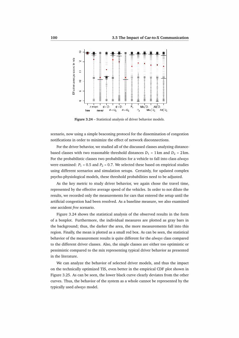
100 3.5 The Impact of Car-to-X Communication
Figure 3.24 – Statistical analysis of driver behavior models.
scenario, now using a simple beaconing protocol for the dissemination of congestion
notifications in order to minimize the effect of network disconnections.
For the driver behavior, we studied all of the discussed classes analyzing distance-
based classes with two reasonable threshold distances D1 = 1 km and D2 = 2 km.
For the probabilistic classes two probabilities for a vehicle to fall into class always
were examined: P1 = 0.5 and P2 = 0.7. We selected these based on empirical studies
using different scenarios and simulation setups. Certainly, for updated complex
psycho-physiological models, these threshold probabilities need to be adjusted.
As the key metric to study driver behavior, we again chose the travel time,
represented by the effective average speed of the vehicles. In order to not dilute the
results, we recorded only the measurements for cars that entered the setup until the
artificial congestion had been resolved. As a baseline measure, we also examined
one accident free scenario.
Figure 3.24 shows the statistical analysis of the observed results in the form
of a boxplot. Furthermore, the individual measures are plotted as gray bars in
the background; thus, the darker the area, the more measurements fall into this
region. Finally, the mean is plotted as a small red box. As can be seen, the statistical
behavior of the measurement results is quite different for the always class compared
to the different driver classes. Also, the single classes are either too optimistic or
pessimistic compared to the mix representing typical driver behavior as presented
in the literature.
We can analyze the behavior of selected driver models, and thus the impact
on the technically optimized TIS, even better in the empirical CDF plot shown in
Figure 3.25. As can be seen, the lower black curve clearly deviates from the other
curves. Thus, the behavior of the system as a whole cannot be represented by the
typically used always model.

3.5 The Impact of Car-to-X Communication 101
Figure 3.25 – Empirical CDF of the average speed achieved for the driverbehavior models.
Figure 3.26 – Q-Q plot of probabilistic vs. mix driver behavior models.
Another remarkable result is that all the shown measures seem to indicate that
the probabilistic model behaves quite similarly compared to the mix models. To
study this effect in more detail, we examined Q-Q plots highlighting the similarity
of these models’ distributions, as shown in Figure 3.26. The closer the points are
matching the diagonal line, the closer the models match. As can be seen, P2 = 0.7
seems to model the mix quite accurately for all scenarios. The key advantage of this
finding is that complex models in experiments and simulations can be substituted
with a probabilistic decision system with only minor impact on the results.
The presented results clearly indicate the need to use realistic driver models,
especially with regard to TIS applications. The presented solution, which has
been integrated into our Veins simulation framework, allows running integrated
simulation experiments taking the driver’s behavior into account.


3.6 Conclusion 103
3.6 Conclusion
In conclusion, it can be said that bidirectionally coupled network and road traffic
simulation provides major advantages compared to uncoupled or purely trace-
driven simulation. Thus, for all protocol evaluations that cannot afford to disregard
network or radio effects and for all evaluations where IVC would likely influence
driver behavior, we strongly advocate the use of bidirectionally coupled simulation.
Only bidirectionally coupled simulations allow for realistic evaluations of the
impact, both directly and indirectly, that Car-to-X communication has on road traffic.
The Veins simulation framework, which we developed, provides all necessary
functionality to perform this bidirectional coupling. The simulation framework
relies on state-of-the-art simulators from both domains: it incorporates well-known
models for road traffic microsimulation with a comprehensive selection of network
protocol models. Using our methodology, we thus provide a means to evaluate
developed protocols more accurately.
The presented study of a Car-to-X communication system’s impact demonstrated
not merely the applicability, but the outright need for bidirectional coupling of road
traffic microsimulation and network simulation.
Quite a number of similar tools [43] have been developed in the last couple of
years that integrate support for realistic mobility models. Most of these tools can,
in theory, also be extended to support the same quality of geodata, performance
metrics, signal propagation models, and route choice models inspired by human
driver behavior. Table 3.4 summarizes some of the most commonly used tools. The
table can be used as a reference if specific IVC applications and protocols are to be
investigated with the help of simulation.
From the lessons learned from more than a decade of IVC simulation, we strongly
advocate to base future studies on such more realistic tools. However, the availability
and accessibility of such tools has often been a problem in the past.
For this reason, we decided to release our Veins simulation framework as Free
and Open Source Software, licensed under the terms of the GNU General Public
License (version 2 or later), and have created a website10 to host the framework and
associated documentation, tutorials, and sample scenarios.
By making Veins available and accessible to the public we actively counter a
trend that is increasingly worrying the network simulation community, namely that
“researchers do not test or document their programs rigorously, and they rarely
release their codes, making it almost impossible to reproduce and verify published
results generated by scientific software” [112].
10http://veins.car2x.org/
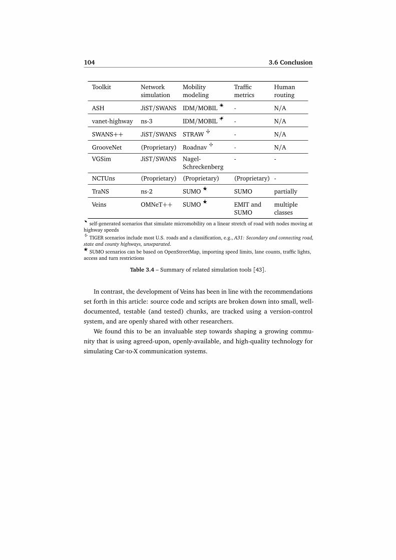
104 3.6 Conclusion
Toolkit Networksimulation
Mobilitymodeling
Trafficmetrics
Humanrouting
ASH JiST/SWANS IDM/MOBIL E - N/A
vanet-highway ns-3 IDM/MOBIL E - N/A
SWANS++ JiST/SWANS STRAW 6 - N/A
GrooveNet (Proprietary) Roadnav 6 - N/A
VGSim JiST/SWANS Nagel-Schreckenberg
- -
NCTUns (Proprietary) (Proprietary) (Proprietary) -
TraNS ns-2 SUMO 8 SUMO partially
Veins OMNeT++ SUMO 8 EMIT andSUMO
multipleclasses
E self-generated scenarios that simulate micromobility on a linear stretch of road with nodes moving athighway speeds6 TIGER scenarios include most U.S. roads and a classification, e.g., A31: Secondary and connecting road,state and county highways, unseparated.8 SUMO scenarios can be based on OpenStreetMap, importing speed limits, lane counts, traffic lights,access and turn restrictions
Table 3.4 – Summary of related simulation tools [43].
In contrast, the development of Veins has been in line with the recommendations
set forth in this article: source code and scripts are broken down into small, well-
documented, testable (and tested) chunks, are tracked using a version-control
system, and are openly shared with other researchers.
We found this to be an invaluable step towards shaping a growing commu-
nity that is using agreed-upon, openly-available, and high-quality technology for
simulating Car-to-X communication systems.

Chapter 4
Engineering Car-to-X Protocols
4.1 Deploying MANET Protocols in VANETs . . . . . . . . . . . . . . . . . 111
4.1.1 Simulation Model . . . . . . . . . . . . . . . . . . . . . . . . . . 111
4.1.2 Simulation Setup . . . . . . . . . . . . . . . . . . . . . . . . . . 114
4.1.3 Performance Evaluation . . . . . . . . . . . . . . . . . . . . . . 118
4.1.4 Conclusion . . . . . . . . . . . . . . . . . . . . . . . . . . . . . . 122
4.2 IVC Systems Based on Cellular Networks . . . . . . . . . . . . . . . . 123
4.2.1 Application Models . . . . . . . . . . . . . . . . . . . . . . . . . 126
4.2.2 Network Models . . . . . . . . . . . . . . . . . . . . . . . . . . 128
4.2.3 Channel Model . . . . . . . . . . . . . . . . . . . . . . . . . . . 129
4.2.4 Road Traffic Model . . . . . . . . . . . . . . . . . . . . . . . . . 132
4.2.5 Performance Evaluation . . . . . . . . . . . . . . . . . . . . . . 133
4.2.6 Conclusion . . . . . . . . . . . . . . . . . . . . . . . . . . . . . . 139
4.3 The Adaptive Traffic Beacon (ATB) Protocol . . . . . . . . . . . . . . . 141
4.4 Design and Characteristics of ATB . . . . . . . . . . . . . . . . . . . . . 145
4.4.1 System Architecture . . . . . . . . . . . . . . . . . . . . . . . . 145
4.4.2 Adaptive Beacon Intervals . . . . . . . . . . . . . . . . . . . . . 145
4.4.3 Flexible Use of Infrastructure Elements . . . . . . . . . . . . . 148
4.4.4 TIS Data Management . . . . . . . . . . . . . . . . . . . . . . . 149
4.4.5 Security and Privacy Issues . . . . . . . . . . . . . . . . . . . . 151
4.4.6 Behavior on a Microscopic Level . . . . . . . . . . . . . . . . . 151
4.5 Performance Evaluation of ATB . . . . . . . . . . . . . . . . . . . . . . 153
4.5.1 Simulation Environment and Parameters . . . . . . . . . . . . 153
4.5.2 Evaluation of Adaptivity . . . . . . . . . . . . . . . . . . . . . . 154
4.5.3 Comparative Evaluation . . . . . . . . . . . . . . . . . . . . . . 157
4.5.4 Realistic City Scenario . . . . . . . . . . . . . . . . . . . . . . . 160
4.6 Comparison of ATB with Flooding/DTN . . . . . . . . . . . . . . . . . 163
4.7 Conclusion . . . . . . . . . . . . . . . . . . . . . . . . . . . . . . . . . . 167
105


4 Engineering Car-to-X Protocols 107
In this chapter, parts of which are based on our articles published in IEEE Commu-
nications Magazine [168], Elsevier Ad Hoc Networks [165], and ACM/Springer Mobile
Networks and Applications [153], as well as presented at conferences and work-
shops [27,152,155,161,166,167], we give examples of how to employ the tech-
niques we presented in the last chapter for simulative performance evaluation of
Car-to-X communication in heterogeneous networks. We first present two examples
of protocol engineering, guided by the historical progression of research in this
domain. These lead us to the design – and an evaluation – of an evolved version of
a beaconing protocol designed for operation in truly heterogeneous environments.
Early inter-vehicle communication approaches concentrated on establishing a
Vehicular Ad Hoc Network (VANET) in its strongest sense, i.e., the application of
routing protocols and coordination techniques known from Mobile Ad Hoc Networks
(MANETs) [148]. The objective was to set up a path between vehicles and – with
the help of pre-deployed infrastructure elements such as Roadside Units (RSUs) – to
a central server.
We investigate such an approach based on the Dynamic MANET On Demand
(DYMO) protocol (cf. Section 2.4.1) in Section 4.1 and show that the main prob-
lem with these solutions is a lack of scalability along multiple dimensions [148].First, messages can only be exchanged with their final destination if a link can be
established (and maintained) to it – yet the stability of links deteriorates sharply
with increasing path lengths. Secondly, this approach only works at sufficient
node densities – yet the node density also has an upper bound, as wireless ad hoc
communication suffers from high collision probabilities in congested areas. Both
problems can be alleviated by deploying additional infrastructure elements, such
as RSUs, which help maintain connectivity and reduce network load, but these
come at high operational costs. Delay/Disruption Tolerant Network (DTN) related
approaches [121] further support connectivity of nodes to a Traffic Information
Center (TIC) by following a store-carry-forward communication principle and data
muling concepts can be applied to Intelligent Transportation Systems (ITS) perform-
ing carry-and-forward of Traffic Information System (TIS) data between vehicles
and such dedicated infrastructure nodes [149].
Another approach to Car-to-X communication systems, and so far the only com-
mercially successful alternative, is the use of cellular networks for information
exchange. Currently available solutions are commonly based on 2G cellular com-
munication networks and recent studies show that special capabilities of 3G/4G
networks (especially the availability of multicast communication), can be benefi-
cial for the operation of Inter-Vehicle Communication (IVC) applications. We thus
investigate such an approach in Section 4.2.
However, it needs to be noted that these solutions are fully dependent on
available network infrastructure elements and only support an efficient downlink to

108 4 Engineering Car-to-X Protocols
the vehicles. Moreover, such IVC approaches frequently rely on a central server that
acts as a sink for new traffic information. This server also transmits the currently
available information (or at least the samples currently relevant to a particular
region) back to the participating vehicles. Such a centralized service can become a
bottleneck or may not be available in some situations [83,146].
The use of cellular networks without the need for a TIC was investigated by
incorporating ideas from the peer-to-peer domain in the peers on wheels vision [138]and further refined in PeerTIS [137]. Conceptually, it is possible to build extremely
robust traffic information systems supporting publish/subscribe interfaces managed
by a Distributed Hash Table (DHT) maintained by the vehicles. Further, the MobTor-
rent approach has been published [25], which also provides mobile (BitTorrent-like)
Internet access from vehicles using RSUs (building on the ideas of drive-thru Inter-
net [121], but exploiting state-of-the-art data management functions).
As a further alternative that can support Car-to-X communications without the
use of any infrastructure, decentralized solutions – one of the most sophisticated
approaches being the Self-Organizing Traffic Information System (SOTIS) [195](cf. Section 2.4.3) – have been investigated.
Common to these solutions is the broadcast of traffic information to neighboring
vehicles, either periodically or triggered by new events [88]. Such traffic information
can be surveyed in a decentralized manner, e.g., based on spatio-temporal data
obtained from vehicle position traces [204]. Multi-hop broadcast is thus a promising
technique, especially for emergency message propagation with delay bounds [134].The dissemination process can also be supported using directed (i.e., geographic)
flooding, which makes lightweight information encoding about both target areas
and preferred routes a necessity [32]. Furthermore, aggregation and other data
pre-processing techniques have been developed to increase the quality of traffic
information and to decrease the associated communication load [98,102,195].
Beaconing, or 1-hop broadcast, is an inherent feature of most of the discussed
systems, one example use being the collection of neighborhood information. The
exploitation of periodic information exchange using such beacons, with special focus
on safety applications, has been analyzed in extensive simulations in [144], showing
that with increasing distance, the success ratio decreases quickly. Combined with
a position based forwarding strategy, however, the approach could be improved.
It was also shown that network load can be significantly reduced by selectively
suppressing broadcasts based on 1-hop neighbor information and that reliability can
be increased via the use of explicit acknowledgments [136]. Most recently, 2-hop
beaconing has been described to acquire topology knowledge for opportunistic
forwarding using the selected best target forwarder [98].
The main challenge for all such beacon systems is that they are very sensitive to
environmental conditions such as vehicle density and network load. A first adaptive
4 Engineering Car-to-X Protocols 109
beaconing system was REACT [185]. Based only on neighbor detection, it can skip
intervals for beacon transmission to support emergency applications. Furthermore,
fundamental scalability criteria need to be considered in order to make the protocol
applicable in the target scenario [142].We believe that beaconing systems are in general well suited for TIS data ex-
change. The key issue is that their optimal configuration is highly dependent on
environmental conditions, e.g., number of vehicles or channel load.
A fully adaptive protocol was thus identified as the next logical step [143,167,
168]. We introduce such a beaconing protocol in Section 4.3, demonstrating how
to cope with the heterogeneity of real world scenarios, how to care for medium
sharing with high priority messages and with other protocols, and how to flexibly
incorporate optional support infrastructure. We conclude with the results of an
evaluation based on a first implementation.


4.1 Deploying MANET Protocols in VANETs 111
4.1 Deploying MANET Protocols in VANETs
In this first example of protocol engineering, we demonstrate a naïve approach
to establishing a system delivering IVC functionality [153,155]: we evaluate the
performance of a system employing existing Internet and MANET protocols, along
with standard hard- and software, to create and maintain a VANET and couple
this network with the Internet. Evidently, this coupling of MANET and Internet is
especially attractive for road users as it allows the utilization of virtually all existing
resources of the Internet without relying on expensive dedicated channels provided
by a cellular network. We thus investigate the feasibility, the performance, and the
limits of such an approach.
As the MANET protocol of choice for this study, we employ the Internet Engineer-
ing Task Force (IETF) MANET working group’s reactive routing protocol candidate,
Dynamic MANET On Demand (DYMO) [24], which we presented in Section 2.4.1.
The DYMO protocol draft expressly provides for the coupling of a MANET with the
Internet, which makes an evaluation of communication connections between mobile
nodes and static infrastructure especially attractive.
4.1.1 Simulation Model
At the time of writing, there were already a few implementations of DYMO available,
mainly for Linux-based systems. Most notable are the DYMOUM (GPL), NIST-
DYMO (public domain), EK-DYMO (closed source), and DYMO-AU (GPL, written in
LUA and C) implementations for the Linux kernel. Furthermore, there is also an
implementation available developed for sensor motes of the Mica series and the
TinyOS operating system: TYMO (GPL, written in nesC).
In the world of network simulation, there exists an implementation of DYMO for
OPNET (proprietary license). Furthermore, the DYMOUM package has been ported
to two of the most commonly used network simulators, ns-2 and OMNeT++. The
DYMOUM package is based on DYMO draft version 05.
Nevertheless, there have been several factors that motivated us to start a new
implementation for OMNeT++. First, the dependency on operating system specific
code leads to some problems in a number of simulation settings. For example,
evaluating DYMO in a sensor network scenario was almost impossible due to the
need to always involve the complete TCP/IP stack. Furthermore, the DYMOUM
package only considered quite an old version of the IETF draft.
Therefore, we started a new implementation of DYMO for OMNeT++ to be used
for research in our group. This model, subsequently called DYMO-FAU, was to be
freely available for use and distribution under the terms of the GPL [151]. Our
simulation model closely followed (and fed back into) the IETF MANET working

112 4.1 Deploying MANET Protocols in VANETs
(a) full-featured (b) minimal
Figure 4.1 – Screenshots of full-featured and minimal MANET nodes runningDYMO, as shown in OMNeT++.
group’s development of the DYMO protocol up until draft version 10. As a main
advantage of this model, we see the applicability in both a fully standard conform
TCP/IP based environment, as well as the parallel availability of a simplified version
of the same code base for use without the complex IP stack. This version can thus
form the basis of a model for evaluating, e.g., ad hoc routing based applications in
sensor networks [36,152].
The DYMO routing protocol was implemented as an application layer module of
the INET Framework module set, which we enhanced to provide netfilter-style hooks
in the network layer, to be used by DYMO in order to maintain a strict separation of
protocol layers. Following the specification [24], it employs UDP to communicate
with other instances of DYMO. The network layer hooks are used for two purposes.
First, they facilitate the queuing of outbound packets before routing in the network
layer occurs, so that a route can be set up by DYMO. The network layer can then be
signaled to release buffered packets for a given destination – either in order to have
them routed to the first hop or to have them discarded because no route could be
found. Secondly, a hook is installed in the inbound packet path. It notifies DYMO of
the arrival of packets. This way, routing table entries can be refreshed and route
errors can be sent. Following the OMNeT++ component model, assembling DYMO
and standard components of the INET Framework to form a simulated MANET node,
illustrated in Figure 4.1a, is a straightforward task.
We outfitted our model of DYMO with the capability to queue payload messages
received from the application layer, should no usable route be known at the time
data is received. As mandated, our model will in this case repeatedly try to establish
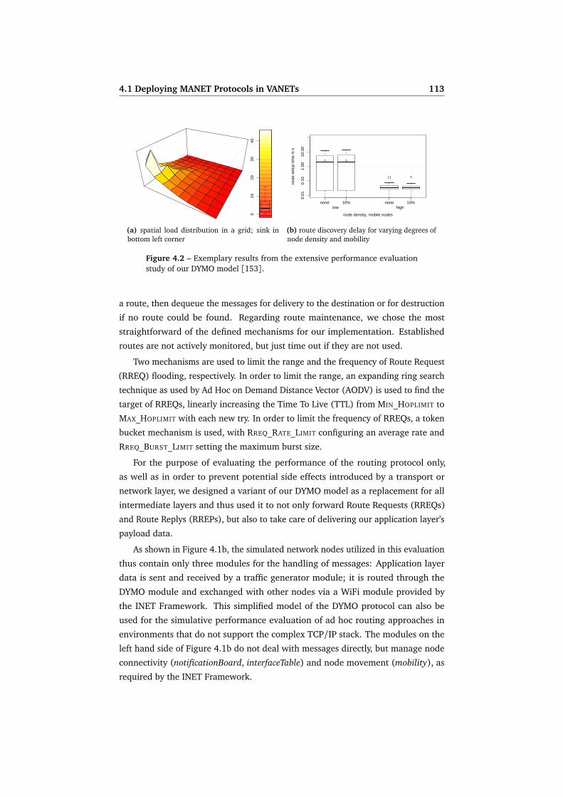
4.1 Deploying MANET Protocols in VANETs 113
010
2030
40
(a) spatial load distribution in a grid; sink inbottom left corner
0.01
0.10
1.00
10.0
0
node density, mobile nodes
rout
e se
tup
time
in s
low highnone 10% none 10%
(b) route discovery delay for varying degrees ofnode density and mobility
Figure 4.2 – Exemplary results from the extensive performance evaluationstudy of our DYMO model [153].
a route, then dequeue the messages for delivery to the destination or for destruction
if no route could be found. Regarding route maintenance, we chose the most
straightforward of the defined mechanisms for our implementation. Established
routes are not actively monitored, but just time out if they are not used.
Two mechanisms are used to limit the range and the frequency of Route Request
(RREQ) flooding, respectively. In order to limit the range, an expanding ring search
technique as used by Ad Hoc on Demand Distance Vector (AODV) is used to find the
target of RREQs, linearly increasing the Time To Live (TTL) from MIN_HOPLIMIT to
MAX_HOPLIMIT with each new try. In order to limit the frequency of RREQs, a token
bucket mechanism is used, with RREQ_RATE_LIMIT configuring an average rate and
RREQ_BURST_LIMIT setting the maximum burst size.
For the purpose of evaluating the performance of the routing protocol only,
as well as in order to prevent potential side effects introduced by a transport or
network layer, we designed a variant of our DYMO model as a replacement for all
intermediate layers and thus used it to not only forward Route Requests (RREQs)
and Route Replys (RREPs), but also to take care of delivering our application layer’s
payload data.
As shown in Figure 4.1b, the simulated network nodes utilized in this evaluation
thus contain only three modules for the handling of messages: Application layer
data is sent and received by a traffic generator module; it is routed through the
DYMO module and exchanged with other nodes via a WiFi module provided by
the INET Framework. This simplified model of the DYMO protocol can also be
used for the simulative performance evaluation of ad hoc routing approaches in
environments that do not support the complex TCP/IP stack. The modules on the
left hand side of Figure 4.1b do not deal with messages directly, but manage node
connectivity (notificationBoard, interfaceTable) and node movement (mobility), as
required by the INET Framework.

114 4.1 Deploying MANET Protocols in VANETs
Parameter Value
MIN_HOPLIMIT 5 hopsMAX_HOPLIMIT 10 hopsNET_TRAVERSAL_TIME 1000 msROUTE_TIMEOUT 5 sROUTE_AGE_MIN_TIMEOUT 1 sROUTE_AGE_MAX_TIMEOUT 60 sROUTE_NEW_TIMEOUT 5 sROUTE_USED_TIMEOUT 5 sROUTE_DELETE_TIMEOUT 10 sRREQ_RATE_LIMIT 10/sRREQ_BURST_LIMIT 3 RREQsRREQ_WAIT_TIME 2 sRREQ_TRIES 3
Table 4.1 – Common parameters of a node running DYMO.
We validated our implementation and conducted an investigation of the perfor-
mance of DYMO in the context of an extensive simulative study, to which we refer
the interested reader [153]. In summary, the results obtained using our model agree
very well with expected values (Figure 4.2a), though we were able to identify cases
where further optimization of the protocol (still in development) was warranted.
Furthermore we were able to demonstrate low route setup delays (Figure 4.2b)
even under node mobility.
The simulation parameters used to configure a DYMO module correspond di-
rectly to the suggested parameter set. They are summarized in Table 4.1, together
with the values used in our evaluation.
4.1.2 Simulation Setup
Conventional ITS are organized in a centralized way. Usually, sensor-based traffic
monitoring systems are deployed directly at the roadside to collect information
about current traffic conditions. Additionally, cars may participate as sensors in
this scenario. The collected data is transferred to one or more dedicated processing
entities, the TIC, where the current road situation is analyzed. The result of this
situation analysis is transmitted to all participating cars via a broadcast medium.
An alternative and completely different approach for monitoring the traffic
situation and distributing the traffic messages to vehicle drivers is to employ a
decentralized self-organizing TIS, in which vehicles inform each other of the local
traffic situation by means of IVC. The traffic situation analysis is performed locally
in each car. No communication infrastructure or additional sensors are required.

4.1 Deploying MANET Protocols in VANETs 115
100
0 m
360
m
Car
Incident
RSU
TIC
(a) centralized communication scenario. IVC issupported by one RSU at each intersection, allconnected to a TIC.
(b) decentralized communication scenario. IVCrelies on VANET alone, leading to multiple iso-lated clusters.
Figure 4.3 – The two types of IVC scenarios for which the performance of adeployed MANET protocol was examined.
We thus use our implementation of DYMO to conduct an evaluation of the
aptitude of MANET protocols for the operation of a VANET in two very different IVC
scenarios: a centralized TIS using pre-installed infrastructure and standard DYMO
routing vs. a decentralized self-organizing TIS relying on UDP based broadcasting
only.
The centralized TIS scenario is depicted in Figure 4.3a. In this scenario, one RSU
is added to each intersection to support IVC, and all RSUs are connected to a central
traffic information service. In this scenario, vehicles employ ad hoc routing to set up
and maintain a TCP connection to the central server, which we use to publish and
revoke incident warnings. In intervals of 60 s or 180 s, depending on the scenario,
vehicles also use this TCP connection to retrieve a list of current incidents from the
central server. We label results from this scenario tic60 and tic180, respectively.
The decentralized scenario is depicted in Figure 4.3b. We realized distributed
behavior by flooding incident warnings through the VANET. Upon receiving an
incident warning, a vehicle queries the originating node if the warning is still
current and, if it receives a positive reply, will try and avoid the lane in question.
Notifications are being flooded over 5 hops or 25 hops, depending on the scenario.
We label results from this scenario 5hop and 25hop, respectively.
In both scenarios incident warnings are triggered as follows: vehicles with a
speed of zero, after some time (in the simulations, we used approx. 1 s for this
delay), try to inform other vehicles of a potential incident on the current lane, using
either of the described mechanisms. If the network simulation determines that
such an incident warning is eventually received by another vehicle, it will store

116 4.1 Deploying MANET Protocols in VANETs
Parameter Value
Maximum vehicle speed 14 m/sMaximum vehicle acceleration 2.6 m/s2
Maximum desired deceleration 4.5 m/s2
Assumed vehicle length 5 mDawdle time 0.5 s
Table 4.2 – Road traffic microsimulation parameters modeling inner-city trafficwith somewhat inattentive drivers.
information about the timestamp and contents of the warning message. Using the
bidirectional coupling to the road traffic simulator, it will also trigger for this vehicle
an adjustment of the affected road segment’s estimated travel time. In addition,
if somewhere along its route the vehicle would have passed this road segment, a
route re-computation is performed using estimated travel times as the cost metric of
Dijkstra’s shortest path algorithm. Vehicles participating in the VANET are thus given
the opportunity to adjust their routes to avoid an incident. When the originating
vehicle resumes its journey, it notifies other vehicles that the lane can be used again,
allowing them to restore their original estimated travel times.
We configured vehicles to drive at a maximum speed of 14 m/s (50.4 km/h,
31.32 mph) and modeled dense inner-city traffic with somewhat inattentive drivers
(setting the Krauß model dawdle time to 0.5 s). Table 4.2 lists the values used to
parameterize the vehicles of the road traffic microsimulation.
For all communications, the complete network stack, including ARP, is simulated
and wireless modules are configured to closely resemble IEEE 802.11b network
cards transmitting at 11 Mbit/s with RTS/CTS disabled. For the simulation of radio
wave propagation, no obstacles are configured and a plain free-space model is
employed, thus leading to best case network topology dynamics. The transmission
parameters of all nodes are adjusted to yield a maximum range of 180 m, a trade-off
between varying real-world measurements described the literature [66,200].
To provide ad hoc routing among nodes, we use the presented implementation of
the DYMO routing protocol as an application-layer module of the INET Framework
module set. As per the specification, it uses a node’s UDP module to communicate
with other instances of DYMO in order to discover and maintain routes and thus
establish a VANET.
All simulation parameters used to parameterize the modules of the INET Frame-
work are summarized in Table 4.3.

4.1 Deploying MANET Protocols in VANETs 117
Parameter Value Parameter Value
TCP.mss 1024 Byte ARP.retryTimeout 1 sTCP.advertisedWindow 14 336 Byte ARP.retryCount 3TCP.tcpAlgorithmClass TCPReno ARP.cacheTimeout 100 s
mac.address auto mac.bitrate 11 Mbit/smac.broadcastBackoff 31 slots mac.maxQueueSize 14 Packets
mac.rtsCts false decider.bitrate 11 Mbit/sdecider.snirThreshold 4 dB
snrEval.bitrate 11 Mbit/s snrEval.headerLength 192 bit.snrThresholdLevel 3 dB .thermalNoise −110 dB
.sensitivity −85 dB .pathLossAlpha 1.9.carrierFrequency 2.4 GHz .transmitterPower 2 mW
channelcontrol.sat −80 dBm channelcontrol.alpha 1.9.carrierFrequency 2.4 GHz .pMax 2 mW
Table 4.3 – INET Framework module parameters modeling IVC-enabled vehi-cles.
Figure 4.4 – Overview of the simulated grid scenario: single-lane roads arelaid out in a grid with a cell size of 1 km2. Start and finish node positionsare fixed. With no IVC, cars always pick the shortest route, illustrated by thedotted line.

118 4.1 Deploying MANET Protocols in VANETs
4.1.3 Performance Evaluation
The scenario that we use for the evaluation is illustrated in Figure 4.4. Single-
lane roads are laid out in a similar fashion to a Manhattan Grid scenario, with
the intersections of roads spaced 1 km apart. This scenario is frequently used for
evaluating protocols designed for urban scenarios – a very good and representative
example is described in [178]. Simulations are performed for grid sizes of 5×5 roads
and 16×16 roads (using 30 and 1000 vehicles, respectively). In each simulation, all
vehicles start, one by one, at a fixed source node in the top left corner of the grid. If
no IVC takes place vehicles then travel along the shortest route to a fixed sink node
located in the bottom right corner of the grid.
Traffic obstructions are introduced by stopping the lead vehicle for 60 s or 240 s,
depending on the scenario. As each road offers a single lane per driving direction,
nodes cannot overtake each other and, hence, need to find a way around blocked
roads by means of IVC, or get stuck in traffic.
In order to provide a detailed look into the effects these obstructions help
manifest in the simulation, Figures 4.5a and 4.5b show the effective average speed
of vehicles, separated by vehicles’ departure times. It was obtained by dividing
the length of the shortest route by each vehicle’s total travel time. Plotted is one
single example run each, for both the case of free flowing traffic and the case of
infrastructure-based IVC with an artificially triggered incident. In the 5×5 grid
scenario depicted in Figure 4.5a, the cars following immediately behind the stopping
vehicle are forced into a traffic jam and delayed accordingly. If the IVC message that
is sent by the stopped car can be received by following cars, they can re-route to a
free road and bypass the jam area.
Similarly, in the 16×16 grid scenario (shown in Figure 4.5b) the incident stopping
the leading car involves a large number of following cars in a traffic jam. This time
some of them are delayed even further. The first cluster of cars that were more than
one road away from the incident, however, already had enough time to receive and
process the incident warning early enough to be able to find alternative routes to
the destination. This allowed vehicles to reach their destination even faster than in
the incident-free scenario, where all just followed the shortest route. As can be seen,
IVC managed to prevent permanent delays on the affected road segment, so even
vehicles that were unaware of the incident were able to continue on their route
shortly after the lead vehicle continued its journey: Up to a departure time of just
over 240 s, their time spent in the jam linearly decreased towards zero.
Vehicles starting later than approx. 65 s and 250 s, respectively, were completely
unaffected by the incident, the only noticeable delays being caused because of
merging traffic flows as vehicles approached their destination.

4.1 Deploying MANET Protocols in VANETs 119
● ● ● ● ● ● ● ● ● ● ● ● ● ● ●● ● ● ●
● ● ● ● ● ● ● ● ● ●●
● ● ● ● ● ● ● ● ● ● ● ● ● ● ●● ● ● ●
● ● ● ● ● ● ● ● ● ●●
0 5 10 15 20 25 30
11.0
12.0
13.0
14.0
Vehicle Departure Time in s
Effe
ctiv
e A
vera
ge S
peed
in m
/s
● freetic60 29
0925
9822
86
Trav
el ti
me
in s
(a) 30 vehicles on a 5×5 grid; lead vehicle stops for 60 s
●●●●●●●●●●●●●●●●●●●●●●●●●●●●●●●●●●●●●●●●●●●●●●●●●●●●●●●●●●●●●●●●●●●●●●●●●●●●●●●●●●●●●●●●●●●●●●●●●●●●●●●●●●●●●●●●●●●●●●●●●●●●●●●●●●●●●●●●●●●●●●●●●●●●●●●●●●●●●●●●●●●●●●●●●●●●●●●●●●●●●●●●●●●●●●●●●●●●●●●●●●●●●●●●●●●●●●●●●●●●●●●●●●●●●●●●●●●●●●●●●●●●●●●●●●●●●●●●●●●●●●●●●●●●●●●●●●●●●●●●●●●●●●●●●●●●●
●●●●●●●●●●●●●●●●●●●●●●●●●●●●●●●●●●●●●●●●●●●●●●●●●●●●●●●●●●●●●●●●●●●●●●●●●●●●●●●●●●●●●●●●●●●●●●●●●●●●●●●●●●●●●●●●●●●●●●●●●●●●●●●●●●●●●●●●●●●●●●●●●●●●●●●●●●●●●●●●●●●●●●●●●●●●●●●●●●●●●●●●●●●●●●●●●●●●●●●●●●●●●●●●●●●●
●●●●●●●●●●●●●●●●●●●●●●●●●●●●●●●●●●●●●●●●●●●●●●●●●●●●●●●●●●●●●●●●●●●●●●●●●●●●●●●●●●●●●●●●●●●●●●●●●●●●●●●●●●●●●●●●●●●●●●●●●●●●●●●●●●●●●●●●●●●●●●●●●
●●●●●●●●●●●●●●●●●●●●●●●●●●●●●●●●●●●●●●●●●●●●●●●●●●●●●●●●●●●●●●●●●●●●●●●●●●●●●●●●●●●●●●●●●●●●●●●●●●●●●●●●●●●●●●●●●●●●●●●●●●●●●●●●●●●●●●●●●●●●●●●●●●●●●●●●●●●●●●●●●●●●●●●●●●●●●●●●●●●●●●●●●●●●●●●●●●●●●●●●●●●●●●●●●●●●●●●●●●●●●●●●●●●●●●●●●●●●●●●●●●●●●●●●●●●●●●●
●●●●●●●●●●●●●●●●●●●●●●●●●●●●●●●●●●●●●●●●●●●●●●●●●●●●●●●●●●●●●●●●●●●●●●●●●●●●●●●●●●●●●●●●●●●●●●●●●●●●●●●●●●●●●●●●●●●●●●●●●●●●●●●●●●●●●●●●●●●●●●●●●●●●●●●●●●●●●●●●●●●●●●●●●●●●●●●●●●●●●●●●●●●●●●●●●●●●●●●●●●●●●●●●●●●●●●●●●●●●●●●●●●●●●●●●●●
●●●●●●●●●●●●●●●
0 100 200 300 400
11.0
12.0
13.0
14.0
Vehicle Departure Time in seconds
Effe
ctiv
e A
vera
ge S
peed
in m
/s
● freetic60 29
0925
9822
86
Trav
el ti
me
in s
econ
ds
(b) 1000 vehicles on a 16×16 grid; lead vehicle stops for 240 s
Figure 4.5 – Average speed of individual vehicles, ordered by time of depar-ture. One scenario with free flowing traffic, one scenario with incident andIVC. Vehicles poll the TIC every minute
In order to examine the broader impact of different IVC setups on communication
performance, we now measure the number of packet collisions on the wireless
channel per packet sent. This metric is often used in the context of analyzing the
efficiency of MANET routing protocols as it describes the effective utilization of
the wireless channel. Figures 4.6a and 4.6b show the results of this evaluation
for small-scale and large-scale simulations, respectively. As can be seen, collision
ratios in the centralized scenarios lead to a substantial packet loss of 10 %, which
could, however, still be compensated by TCP retry mechanisms. Collision ratios in
decentralized scenarios, on the other hand, exceeded 25 % in large-scale simulations,
which massively hindered packet exchanges.

120 4.1 Deploying MANET Protocols in VANETs
●●●●●
●●
free none tic180 tic60 25hop 5hop
0.0
0.2
0.4
0.6
0.8
1.0
Col
lisio
ns p
er P
acke
t Sen
t
(a) 30 vehicles on a 5×5 grid; lead vehicle stops for 60 s
●
●●●●
●●●●●●●●●
●
●●●
●
●●●
●●
●●●●●●●
●
●●●●●●●
●
●●●
●
●
●
●●●
●
●●●
●
●
●
●
●
●●●
●
●●
●
●●●
●●●●●●●●●●●●●●●●●●●
●●●●●●● ●●
●●●●●●●●●●●●●●●●●●
free none tic180 tic60 25hop 5hop
0.0
0.2
0.4
0.6
0.8
1.0
Col
lisio
ns p
er P
acke
t Sen
t
(b) 1000 vehicles on a 16×16 grid; lead vehicle stops for 240 s
Figure 4.6 – Packet collisions on the wireless channel per packet sent. Onescenario with free flowing traffic, one with no IVC, four scenarios with differenttypes of VANET communication.
These results are also reflected in the impact different IVC setups had on road
traffic performance. Plotted in Figures 4.7a and 4.7b is the effective average speed
of vehicles, measured in small and large-scale simulations, respectively.
As can be seen, in the case of free flowing traffic, the travel time distribution
among simulated vehicles in both scenarios is almost homogeneous, as could be
expected, but speeds average at well below the maximum speed of 14 m/s. This is
due to cars decelerating at every intersection, which, in combination with high traffic
densities on the single, shortest route shared by all vehicles, leads to micro-jams. In
the second case, where the lead vehicle is being stopped for a short amount of time
(simulating, e.g., an accident), without IVC taking place, the average node speed is
reduced by both this stop and by the traffic jam left behind.

4.1 Deploying MANET Protocols in VANETs 121
●
●●
●●
free none tic180 tic60 25hop 5hop
1011
1213
1415
Effe
ctiv
e A
vera
ge S
peed
in m
/s
(a) 30 vehicles on a 5×5 grid; lead vehicle stops for 60 s
●●●●●●●●●●●●●●●●●●●●●●●●●●●●●●
●●
●●●●●●●●●●●●●●●
●●●●●●●●●●●●●●●●●●●●●
●●●●
●●
●●
●●●●●●
●●●●●●●●●●●●●●●●
●●
●●●●●●
●●
●●●●●●●●●●●●
●
●●●●
●●●●●
●
●●●●●
●●●●●●●
●●
●●●●●●●●●●●
●
●●●●●●●●
●●●●●
●●●●●
●●●●
●●●●●●●
●●
●
●
●●●●●●●●●●●●●●●●●●●●●●●●●●●
●●●●●●●●●●
●●●●
●
●●●●
●●●●●●●●●●●●●●●●●●●●●●●●●●●●●
●
●●●●●●●●●●●●●●●●●●●●●
●
●●
●●●
●
●●●●●●●●●●●●●
●
●
●●
●●●●●●
●●●●●
●●●●●●●●●●●●●●●●●●●●●●
●●●●
●●●●●●●●●●●●
●●●●●
free none tic180 tic60 25hop 5hop
1011
1213
1415
Effe
ctiv
e A
vera
ge S
peed
in m
/s
(b) 1000 vehicles on a 16×16 grid; lead vehicle stops for 240 s
Figure 4.7 – Vehicle speed averaged over all vehicles. One scenario with freeflowing traffic, one with no IVC, four scenarios with different types of VANETcommunication.
We now examine the influence of the two different Car-to-X communications
paradigms on traffic performance as a whole. In the small-scale simulation of
Figure 4.7a, a polling interval of 180 s for centralized communications proved too
long to substantially influence road traffic performance, but a polling interval of
60 s already led to a noticeable improvement. Performance was even better for
decentralized communication scenarios, where almost a quarter of vehicles did not
suffer increased travel times due to the simulated incident if the TTL was reduced
to 5 hops.
In the large-scale simulations of Figure 4.7b, results were almost reversed.
Here, decentralized communications could only marginally improve road traffic
performance and centralized communication scenarios fared far better. When a

122 4.1 Deploying MANET Protocols in VANETs
small polling interval was used, almost all vehicles reached their goal even faster
than they could in the case of unobstructed traffic without IVC, thanks to a large
number of vehicles taking alternate routes, which reduced traffic densities and
helped avoid micro-jams.
4.1.4 Conclusion
Evaluation of the feasibility and the expected quality of VANETs operated with the
routing protocol DYMO showed that, at low densities (e.g., for low penetration
rates) the examined approach is clearly inferior to even a simple flooding protocol.
Here, the overhead of flooding management messages through the network to set
up very short lived routes proved too wasteful to support the operation of an IVC
system.
For small amounts of payload data to be transported and high traffic densities,
however, it can be used to successfully set up and maintain ad hoc networks of
vehicles and roadside infrastructure, even though it still causes disproportionate
network load.
Still, it bears repeating that this study on the performance of DYMO-supported
IVC systems was based on best case topology dynamics (i.e., no obstacles blocking
radio communication) as well as an assumed 100 % penetration rate with IVC
technology and dedicated VANET infrastructure (i.e., every vehicle was outfitted
with IVC equipment and every intersection was outfitted with an RSU).
As it is extremely costly to retrofit existing roads with such dedicated VANET
infrastructure, an investigation of the aptitude of existing general-purpose commu-
nication infrastructure, i.e., cellular networks, might therefore prove worthwhile.

4.2 IVC Systems Based on Cellular Networks 123
Road Traffic Model
Application Model
Channel Model
Core Net Model
PDN Model
Application Model
RAN Model
FTAPFTAP TPEGTPEG
Figure 4.8 – Component model of the simulated UMTS-based Car-to-X com-munication system.
4.2 IVC Systems Based on Cellular Networks
The first commercial versions of what could be described as early Car-to-X commu-
nication systems based on 2G cellular networks are already available to customers
today, but they are facing low network throughput and high operational costs,
hindering their adoption as the basis for true IVC systems.
3G telecommunication networks, specifically the Universal Mobile Telecommuni-
cations System (UMTS), are a relatively new player in the field of IVC [140,184]and offer a couple of benefits for IVC applications. Owing to their system design,
in conjunction with much larger data rates compared to 2G networks, IVC system
operation based on 3G networks becomes economically feasible. In addition, unlike
infrastructure-assisted solutions using WiFi or WiMAX, UMTS-based solutions can
rely on readily-available infrastructure.
Compared to WiFi-based IVC solutions, however, the perceived strengths and
weaknesses of UMTS networks are quite different. While, for example, the security
of infrastructure-less networks cannot easily be guaranteed [133], there already are
strong security measures in place to guarantee 3G networks’ integrity, which can be
re-used for Car-to-X communication. As a second example, the distance between a
message’s sender and its intended receivers is almost a non-issue in 3G networks:
its impact on the end-to-end delay is negligible. On the other hand, even for short-
distance messages the end-to-end delay is already quite high compared to that of

124 4.2 IVC Systems Based on Cellular Networks
direct radio links. A key question to be asked about a UMTS-based IVC system is
therefore whether end-to-end delays will still be acceptable not only for common TIS
applications, but also for the transmission of hazard warnings. Another important
question is whether such a system will scale better [61] than more traditional
WiFi-based infrastructure-less solutions to accommodate high penetration rates,
given that in this solution all network traffic has to be routed through the available
infrastructure.
Together with obvious business reasons, both questions are at the core of the
problems which hindered adoption of some of the early 2G-based approaches [206]to Car-to-X communications via a cellular network proposed in the 1990s. Devel-
opment of cellular network based solutions is now picking up again, with new
approaches based on 3G networks.
The state of the art in cellular communication already allows for interesting and
proven applications in the domain of ITS, one such application being the derivation
of estimations on traffic density from passively acquired cellular network data and
its distribution to end users within minutes, marketed as, e.g., the TomTom HD
Traffic service. Moreover, new technologies in UMTS networks promise delays of
less than one second while at the same time reducing network load.
Recent work in this field has mainly dealt with analytical evaluations of only
some of such a communication system’s aspects [184]. By means of an analytical
model, the authors quantified the achievable performance in some realistic scenarios.
In particular, the advantages of the Multimedia Broadcast Multicast Service (MBMS)
extension to UMTS were studied, which is needed to support efficient infrastructure-
based IVC services on top of the UMTS network if the number of users is high [10].Although MBMS is still lacking widespread commercial adoption, interoperability
tests and several trials in operators’ networks have already proven the standard
ready for adoption.
Experimental approaches have accomplished post-hoc analysis of implemented
testbeds using state of the art technology. In these setups, either detailed studies
have been conducted [140] or complex extensible testbed architectures have been
developed [129]. However, only the currently deployed UMTS versions could be
tested and the size of the experiments was limited. Moreover, an evaluation of the
broader impact of a TIS based on real-world experiments is infeasible, and even
simulative studies on this topic are rare [31].
Simulation experiments of UMTS networks are usually performed using propri-
etary models without focus on application in vehicular environments (e.g., in [7])and without incorporating realistic mobility models. Furthermore, such simulations
are not using a holistic approach, i.e., they are not including all system aspects from
the wireless links to the core 3G network as well as influence of the road traffic, yet

4.2 IVC Systems Based on Cellular Networks 125
even for WiFi-based infrastructure-less approaches it has been shown that coupled
simulation of network communication and road traffic is necessary [156,169].
Comprehensive evaluations of such vehicular communication systems, as well
as using features which are still in the early planning stages, can, however, be
performed if all components of such a system are modeled in sufficient detail
and assembled into one simulation. Therefore, we extended our Veins simulation
framework to allow for a holistic analysis of a complex 3G-based TIS.
Our simulation framework now includes a set of customized application layer
protocols, to be used in both the up- and downlink direction. These protocols
benefit from new features of cellular communication systems, e.g., High Speed
Packet Access (HSPA) which improves up- and downlink data rates and transmission
latencies. For easy integration into existing, standardized communication systems,
these protocols are implemented on top of the cellular communication protocol
stacks.
Veins could thus be used for the simulative evaluation of the planned real-world
IVC system based on cellular networks designed in the Cooperative Cars (CoCar)
project [59]. CoCar is a sub-project of the German government funded research
initiative Aktiv,11 which encompasses research in the fields of traffic management,
active vehicle safety, and cooperative systems. Aside from examining the technologi-
cal feasibility of such a system, CoCar also addresses establishing a solid business
case [38].
In this case study [165] we show simulation results for a typical highway
scenario based on real-world 3G network coverage data. The results clearly outline
the capabilities of the simulation framework and the collected metrics could be
shown to match small-scale field operational tests, as well as to be consistent with
expectations of a large-scale rollout.
Figure 4.8 depicts an overview of the planned CoCar communication system,
along with the various models that have been integrated to form the testbed we
use for evaluations. Guided by this figure, we describe in the following each of the
models the framework is composed of and detail how the models interact with each
other.
First, Section 4.2.1 introduces the application models. Section 4.2.2 gives an
overview on the Internet, core network, and radio access network models used.
Section 4.2.3 details the UMTS channel model that was integrated with the simulator
and Section 4.2.4 introduces the road traffic model. Finally, the results that we
obtained in a simulative performance evaluation are outlined in Section 4.2.5,
focusing on the use case of traffic jam warning exchange.
11http://www.aktiv-online.org/
126 4.2 IVC Systems Based on Cellular Networks
4.2.1 Application Models
In the simulation framework, components at the network edge are represented
using detailed application-layer models of the respective services. These components
are the TIC and the CoCar-enabled vehicles. Both send and act upon bit-precise
representations of CoCar messages.
Three application-layer protocols have been specified in order to handle com-
munication among vehicles in the CoCar system. The first one, the Traffic Probe
Data Protocol (TPDP), is a lightweight binary protocol that serves to provide regular
traffic condition updates to the server. As stated, we are focusing on the use case of
warning message exchange, so in the simulation model only the two other protocols
were deployed.
As illustrated in Figure 4.8, vehicles use the Fast Traffic Alert Protocol (FTAP) to
send messages to the CoCar TIC. FTAP messages are sent in a very compact, binary
representation. In the downlink, these messages are quickly broadcast to all vehicles
in the same cell, again using the FTAP protocol.
This is achieved by dedicated infrastructure components installed close to the
base stations, which we term the CoCar reflectors. These components are able to
pass received FTAP messages to the TIC, but also to autonomously relay them back
to the originating cell.
In a second step, the TIC aggregates all received messages’ contents to maintain
a higher-level view on traffic conditions, potentially integrating information from
external sources. From this high-level view, a pool of CoCar messages is then
derived.
These messages are using a message encoding based on that of the Transport
Protocol Expert Group (TPEG) protocol suite, which defines a standardized means
for traffic data exchange between cooperating parties and with end users. CoCar
messages were integrated with this suite, specifying missing CoCar information
elements to create a TPEG-conformant message type [27], called an application in
TPEG terminology. This CoCar application builds upon, but is independent from
other standardized TPEG applications.
Thus, CoCar application messages are formatted using XML and are conformant
to the TPEG XML protocol standard series [180]. By this means, CoCar messages
can be very flexibly handled: On the one hand, they can be used alone, without
any other TPEG application; on the other hand, they can be easily integrated into a
TPEG message stream and transferred to the clients using other applications. Traffic
messages in the pool are then periodically geocast in the form of a TPEG carousel.
Figure 4.9 illustrates the modular buildup of a CoCar-enabled vehicle from
logical components, which realize the functionality described in the following. The
CoCar specific protocol is built upon the IP and UMTS protocol stacks.

4.2 IVC Systems Based on Cellular Networks 127
Figure 4.9 – OMNeT++ representation of a CoCar-enabled vehicle in UMLnotation.
The selection of transport layer protocols, such as UDP or TCP, depends on the
functional requirements as well as on performance requirements of the applications,
like the message transmission delay.
Vehicles in the simulation model receive traffic information messages via modules
representing a UMTS card and keep a record of traffic conditions. They are also
configured to continuously monitor the state of their mobility module. When the
node is detected to have inexplicably stopped for an extended period of time, it
assumes that a traffic jam has occurred. In the application-layer module, a vehicle
then generates a traffic message and sends it via its UMTS card to the TIC under two
conditions: The vehicle did not yet receive a similar incident warning and enough
time has passed since the incident was detected to compensate for the round trip
time of traffic messages that might be underway.
The TIC of the simulation model serves as the CoCar system’s core component
which can collect and process CoCar specific application messages from authorized
cars and from auxiliary traffic and travel information service providers. As shown
in Figure 4.8, the TIC is located outside the UMTS core network, connected via the
Internet. It thus communicates with vehicles via the UMTS core network components
and provides interfaces to other service providers.
In order to obtain realistic results, application layer models employed techniques
to avoid unnecessary message transmissions, such as micro-aggregation of FTAP
messages at the server side prior to them being re-broadcast to the same cell and
client-side duplicate avoidance by keeping track of what was already reported to
the TIC.

128 4.2 IVC Systems Based on Cellular Networks
Several parameters were introduced that allowed for a fine-tuning of the applica-
tion layer models’ behavior to optimize their performance. Among these configurable
aspects are:
• variable FTAP and TPEG message configurations to examine trade-offs be-
tween system performance and different message and header lengths, e.g., to
provide support for security elements,
• bandwidth limits to be observed by the TIC to examine the impact of CoCar
transmissions on the core network vs. reduced delays,
• freely-configurable message repeat intervals and validity timeouts to examine
how best to balance network load and dissemination speeds, and
• architectural variants of the communication infrastructure, to help judge in
what direction core network components of the UMTS should evolve.
4.2.2 Network Models
The number of parallel unicast connections in UMTS is limited by the cell size: The
distance between a mobile terminal and its associated UMTS base station (i.e., the
NodeB) determines the path loss for the radio connections. A vehicle that is far
from the cell’s center will require a higher transmit power to communicate with the
NodeB. This, in turn, increases the overall interference level of the cell. Since UMTS
is an interference limited system, this reduces the number of possible simultaneous
connections in the cell, eventually leading to new connection requests being blocked.
In order to avoid unrealistic simulation setups, nodes representing UMTS base
stations were therefore set up in the simulated area according to real-world 3G
network coverage data courtesy of Vodafone Group R&D Germany, with typical cell
sizes ranging from 500 m in populated areas to approx. 4500 m in the countryside.
Three network elements are used to transmit messages received at the NodeBs
to the communication system’s TIC. All NodeBs are connected via the radio access
network to the UMTS provider’s core network components. These components relay
messages via the core network to a Gateway GPRS Support Node (GGSN), where
they are commonly re-framed for transmission over a public network and to their
destination, namely the TIC.
Algorithms for packet scheduling and optimization are the intellectual properties
of network operators and the actual network design varies widely between different
implementations. In our simulation framework, both the radio access network and
the core network components are therefore simulated at an abstract level: All base
stations were transparently connected to a node representing the GGSN and the

4.2 IVC Systems Based on Cellular Networks 129
processes of message scheduling and transmission were reproduced using statistical
models of the radio access network and core network.
However, all protocol adaptation and re-framing at this gateway node was per-
formed using the well-tested models of the OMNeT++ INET Framework extension
for Internet models. This made it possible to simulate the channel between gateway
and TIC using detailed models of an Ethernet link and network cards, as well as all
protocol layers up to the transport layer.
4.2.3 Channel Model
Actually performing all signal processing tasks that take place on the UMTS physical
layer for every single network connection is infeasible in terms of computational
effort and memory consumption. Instead, performance measures should ideally be
modeled on a higher level.
Therefore, realistic simulation of UMTS channels was accomplished by employ-
ing a dedicated link level simulator and performing extensive simulations of packet
transmissions off-line. In the following, we detail how a set of statistical models
was derived from the results of these simulations to serve as the basis of a simula-
tion module modeling packet errors and delays encountered during UMTS packet
transmissions.
Channel quality in the UMTS system has a dependency on vehicle speed, which
is a continuous figure. Thus, for the simulations, a set of discrete vehicle speeds was
picked and for each (as well as for all combinations of remaining input parameters)
a separate set of simulation results was computed. Subsequently, the results of these
simulation experiments were used to derive distribution functions for all involved
statistic variables.
For each radio transmission to be evaluated in the target simulation framework,
the simulation module could then interpolate between the two most closely matching
distribution functions for a vehicle’s speed and for the current communication
parameters to arrive at a packet error rate and the transmission’s delay and duration.
4.2.3.1 Random Access Channel (RACH)
The simulation results (Figure 4.10) depict the distributions of delay times that can
be expected for various RACH parameter settings. Specifically, the delays consist
of the time that passes between message generation in the mobile terminal, the
subsequent power ramping phase, and the correct detection of the access preamble
by the NodeB.
Table 4.4 shows the parameters that were used in the overall performance
evaluation. The solid black line of Figure 4.10 represents those default parameters,
whereas the other curves were generated by varying a single parameter each. All

130 4.2 IVC Systems Based on Cellular Networks
Spreading Factor 32No. of receive antennas 1Vehicle speed 0 km/h . . . 130 km/hPower step 2 dBNo. of sub-channels 2Size of message 70 Byte
Table 4.4 – Default set of parameters for the RACH.
0 20 40 60 80
0.0
0.2
0.4
0.6
0.8
1.0
time until correct preamble reception in ms
CD
F
default
2 RX antennas
3 dB power step
4 subchannels
Figure 4.10 – Empirical CDF of the random access procedure duration for thedefault set of parameters (c0=−6 dB, 2 dB power step, 1 RX antenna, 2 RACHsubchannels), compared to alternative parameterizations.
simulations use the ITU Vehicular B power delay profile for modeling multipath
fading. Transmission times for data are not included in the figures. Since these are
deterministic values, they can be added as a constant factor as needed.
The simulation studies show that the access times for the RACH can be influenced
by operator-chosen parameters as follows. The number of sub-channels that is
available for a particular service determines the frequency of the allowed access
attempts and, therefore, the capacity of the RACH. Increasing the number of RACH
sub-channels has shown to yield a linear gain in latency, at no additional cost.
However, it should be noted that there are only a total of 12 sub-channels available
for all services and that a minimum of 3 access slots, which equates to 4 ms, must
remain unused between two consecutive access attempts [1]. In the following, we
therefore assume two sub-channels to be allocated.
The power step size must be chosen rather carefully. For a single user, a larger
step size will increase the probability for each preamble to be successfully detected

4.2 IVC Systems Based on Cellular Networks 131
by the NodeB. Nevertheless, in a typical multi-user scenario, the interference caused
by access attempts will negatively affect transmissions of other users, thus increasing
delay times. The power step size can be chosen from a range of 1 dB . . . 8 dB, with
1 dB steps [2]. As a trade-off, we assume a power step size of 2 dB.
Finally, the number of receive antennas of the NodeB is taken into account. As
can be seen from Figure 4.10, NodeBs equipped with antenna arrays will be able
to achieve a considerable gain in detection performance, which can greatly reduce
delay times on the air interface. Still, we assume a conservative configuration with
one receive antenna.
Although this choice of parameters is rather conservative, our system is able to
maintain sufficient QoS to support even time-critical applications, as we will show in
the following. As mentioned, the solid black curve (labeled default) in Figure 4.10
depicts the delay distribution for this specific set of parameters. Obviously, 90 % of
all access procedures take about 55 ms or less to complete. Using a spreading factor
of 32 results in a data rate of 120 kbit/s on the physical layer, or 150 Byte per frame.
The duration of a frame is 10 ms.
Taking into account the channel coding and overhead from the higher protocol
layers, we find that the 70 Byte message cannot be transmitted during one frame but
must be split into two. Subsequently the total delay for 90 % of all access procedures
can be calculated according to Equation (4.1).
45 ms + 2 × 10 ms = 65 ms. (4.1)
Messages that do not fit into two radio frames would have to be split further
and a new access procedure is required after each two consecutive frames, which
will again increase the time to complete the data transmission. Therefore, in the
CoCar system only FTAP messages, which will fit into at most two RACH frames, are
transmitted via the RACH.
4.2.3.2 Forward Access Channel (FACH)
In the Forward Access Channel (FACH) simulation model we used, transmission of
a message of size n on this channel can be calculated according to Equation (4.2).
t = ⌈ n40 Byte
⌉ × 10 ms (4.2)
This is because messages are transmitted on the FACH in discrete slots of 10 ms
each. Implementers of the FACH can choose between a number of different slot
formats, detailed in [3]. This results in different spreading factors being used and
different channel bit rates being available for transmissions. In our evaluations,
we assume a FACH parameterization that allows 40 Byte of data to be sent in one
frame.

132 4.2 IVC Systems Based on Cellular Networks
Figure 4.11 – Road map of the 10 km × 10 km simulation scenario and GUIscreenshot of the traffic simulator, showing a subsection of the freeway inter-change during the simulation.
Ideally, multicast downlink messages in the CoCar system are therefore transmit-
ted over the UMTS FACH. If no multicast capability is present in the communication
system, UMTS Dedicated Channels (DCHs) are used.
4.2.4 Road Traffic Model
Serving as communication scenario of the proof-of-concept evaluation was traffic
in the area of a large freeway interchange next to Frankfurt Airport. This region,
where two major German freeways (A 3 and A 5) and one large highway (B 43)
connect, was chosen because of its overlap with the testbed of the German research
initiative simTD [174] and because of the challenges it poses to routing and traffic
optimization. Figure 4.11 gives an overview of the scenario, which spans an area of
approximately 10 km × 10 km. In this area, all traffic on roads classified as Autobahn,
Schnellstraße, and Bundesstraße (freeway, expressway, and highway) was simulated.
Traffic flows of 2000 vehicles were set up in the east-west and west-east directions
of freeway A 3, keeping the number of simulated cars manageable, but at the same
time allowing for a multitude of alternative routes, e.g., along highway B 43.
The mobility models of nodes were configured to model two distinct vehicle
classes, loosely representing cars and trucks, their parameters set to the values given
in Table 4.5.

4.2 IVC Systems Based on Cellular Networks 133
Parameter Car Truck
Fraction of vehicles 80 % 20 %Mobility model Krauß Krauß
Maximum speed 35 m/s . . . 70 m/s 22 m/s . . . 28 m/sMaximum acceleration 2.60 m/s2 1.30 m/s2
Desired deceleration 4.5 m/s2 4.0 m/s2
Assumed length 5 m 15 mDawdle time 0.5 s 0.75 s
Table 4.5 – Road traffic microsimulation parameters modeling a mix of carsand trucks.
This parameter set lead to a diverse mix of vehicles participating in the scenario,
which in turn lead to very dynamic traffic patterns emerging during simulations.
A lane-precise road network model was employed, based on geodata available via
OpenStreetMap, as presented in Section 2.2.4.
Realistic movement of cars was achieved by first iteratively applying the Dynamic
User Assignment (DUA) algorithm [54] for the computation of routes for all vehicles
until a steady state regarding route selection was achieved. The mobility scenario
was then modified by adding an artificial traffic obstruction, namely the closing of
two out of three lanes at the freeway interchange, preceded by a short subsection
of freeway that imposed a 60 km/h speed limit on all vehicles. No adjustment of
pre-computed routes was performed for this modified scenario, so all vehicles started
out unaware of the presence of the obstruction. This way, the traffic pattern in
the vicinity of the obstruction quickly reached congested conditions with densities
peaking at 365 vehicles within the service area of one UMTS cell. Vehicles could
then use the CoCar communication system to exchange information about perceived
traffic jams, causing all receivers of such a warning to adjust their routes to avoid
affected roads.
In order to compare mobility scenarios in terms of smoothness of traffic and the
associated environmental impact, we rely on the emission metrics provided by Veins,
which are based on the EMIT model presented in Section 3.2.
4.2.5 Performance Evaluation
The first and foremost benefit of any TIS is, of course, the increase in overall road
safety which it can effect not only by assisting users (e.g., with route planning), but
also by providing early and accurate jam and hazard warnings. Secondly, a TIS can
facilitate dynamic re-distribution of traffic, decrease local traffic densities, and thus
lead to smoother traffic. However, operational parameters of a UMTS-based TIS (in
particular when optimizing for timeliness of messages) have to be balanced with

134 4.2 IVC Systems Based on Cellular Networks
the load it will exhibit on the network infrastructure, which is shared with other
applications.
In the following, we outline selected results from multiple runs of simulative
performance evaluations of these three problem domains, obtained by modeling
the interworking scenarios of communications and road traffic in an IVC system
based on cellular networking. In particular, we provide answers to the following
questions:
• Will the system strike a balance between smoothing traffic and at the same
time not send vehicles on unnecessarily long detours? As the quality of this
balance is directly reflected in overall traffic emissions, we first examine the
impact system operation has on CO2 emissions.
• How much strain will different system configurations put on the network
infrastructure? What is the network load on the air interface, the core network,
and on the servers?
• How timely will vehicles learn about a new event, either in the immediate
vicinity or at an arbitrary location? What end-to-end delay can be expected
for messages received via FTAP or via TPEG?
4.2.5.1 Impact on road traffic
Figure 4.12 shows the results of the first evaluation, examining the impact of the
CoCar communication system on the environment. It plots the empirical CDF of all
vehicles’ total amount of CO2 emitted during their travel from start to destination,
independent of the length of their route. As can be seen, activating the CoCar
communication system in simulations did not lead to an increase in participants’
CO2 emissions, as could be assumed based on the much longer detours that vehicles
would now routinely take to reach their destination. Instead, a slight decrease was
observed – from a median of approx. 1755 g per vehicle and a total of 3780 kg to a
median of 1679 g and total of 3740 kg. This is also indicative of a smoother traffic
flow.
4.2.5.2 Impact on network traffic
Aside from the impact the CoCar communication system might have on road traffic,
it is just as important to know how the rollout of such a system would affect
existing services – in particular with regard to the allocation of network resources to
the CoCar system. As the availability of MBMS (and, hence, a multicast message
dissemination service) was expected to have a large impact on system load and
delays, the following evaluations have been performed for two different parameter
sets each, modeling a system with and without MBMS capability.

4.2 IVC Systems Based on Cellular Networks 135
0.0
0.2
0.4
0.6
0.8
1.0
CD
F
CoCar system disabled
CoCar system enabled
total CO2 emission of vehicles in g
0 1000 2000 3000 4000
1679
1755
Figure 4.12 – Impact of the CoCar communication system on road traffic:Quantiles of vehicles’ CO2 emissions; empirical CDFs and median values.
Figure 4.13 illustrates the impact of the CoCar system on network traffic – both
in the core network and on the air interface. Figure 4.13a shows an example of the
network resources used by the CoCar system depending on the system configuration,
plotted as an empirical Cumulative Distribution Function (CDF) of the average data
rate of transmissions from the TIC, i.e., data sent to the core network. As can be
expected, the relations between message size, carousel size, and allocated maximum
network resources lead to a bursty traffic pattern. In the unicast case, network load
was heavy, easily reaching approx. 7000 kbit/s, with the typical system load still
exceeding 2000 kbit/s. In a system with MBMS capabilities, the median of network
load yielded a much lower 2.5 kbit/s and the 90 % quantile yielded only 6 kbit/s.Figure 4.13b shows a similar plot, but illustrates the average data rate of trans-
missions from CoCar clients, i.e., data sent on the RACH. Here, client-side duplicate
avoidance lead to a sparser utilization of the available channel, with network re-
source utilization in a unicast-only system remaining below 300 kbit/s and, more
importantly, utilization of the MBMS-capable system yielding a 90 % quantile of
under 0.2 kbit/s and a median value near 0 kbit/s.Extrapolating these results for a nationwide communication system, even when
keeping in mind that the measures recorded in this simulation only reflect the
quantity of data transmitted for an area of less than 10 km × 10 km, these results
are very promising. In the end, most of the accumulated data is only relevant for

136 4.2 IVC Systems Based on Cellular Networks
0.0
0.2
0.4
0.6
0.8
1.0
CD
F
unicast scenario
multicast scenario
outbound traffic of TIC in Mbit/s
0 2 4 6 8 10
0.006
6.9819
(a) Downlink to vehicles
0.0
0.2
0.4
0.6
0.8
1.0
CD
F
unicast scenario
multicast scenario
inbound RACH traffic at NodeBs in Mbit/s
0.00 0.05 0.10 0.15 0.20 0.25 0.30
0.0001
0.2589
(b) Uplink to TIC
Figure 4.13 – Impact of the CoCar communication system on network traffic;empirical CDFs and 90 % quantile.

4.2 IVC Systems Based on Cellular Networks 137
the area it was recorded in and, given appropriate infrastructural support, need not
be transmitted globally.
4.2.5.3 End-to-end delays
From an end user perspective, one of the most important measures to be recorded for
the CoCar communication system is that of end-to-end delays. Often, the end-to-end
delay is the one key figure that determines whether certain applications are feasible
in a system – or if they simply cannot be realized because information would not
reach its addressees in time.
These measures are plotted in Figure 4.14 for the TPEG and FTAP message types
and for three different parameter sets. Again, the first parameter set represents
a communication system incapable of performing MBMS services. The second
and third parameter sets both model an MBMS-capable system and illustrate the
trade-off between on the one hand reducing delay in the direct vicinity of traffic
incidents, and on the other hand increasing the delay that wide-range dissemination
of information will suffer.
Figure 4.14a shows the delay between a warning message being sent by one ve-
hicle and its associated TPEG traffic information message being received by another.
Not counted is the time for cars that had not yet entered the simulation area when
the message was sent and were as such fundamentally unable to receive it. Also
explicitly not reflected in this figure are messages containing information that was
already known to cars, e.g., because they had been received via FTAP by the time a
TPEG message was received.
For the first parameter set (a system performing only unicast transmissions
of messages in the downstream) noticeable end-to-end delays were experienced
by most vehicles, with delays of up to 21 s for the fastest 90 % of transmissions.
For an MBMS-enabled system, however, 90 % of messages could be seen to have
experienced end-to-end delays of under 10 s with 75 % of messages experiencing no
more than a 1 s delay. Still, even in this case, for 10 % of messages it took up to one
complete carousel repetition interval until they were received by all vehicles. In the
baseline scenario, this means that messages may take up to slightly over 30 s (in the
case of doubled warning intervals slightly over 60 s) until wide-area dissemination
of a message is attained.
Similarly, Figure 4.14b shows the delay between a warning message being sent
by one vehicle and the re-sent FTAP message being received by vehicles in the same
cell. Once again, this measure only includes transmissions for cars that had already
entered the simulation area and which had not already been informed about the
particular congestion.

138 4.2 IVC Systems Based on Cellular Networks
0.0
0.2
0.4
0.6
0.8
1.0
CD
F
multicast scenario
multicast, double carousel length
unicast scenario
TPEG end to end delay in s
0 10 20 30 40 50 60
2124
10
(a) Messages via TPEG
0.0
0.2
0.4
0.6
0.8
1.0
CD
F
multicast scenario
multicast, double carousel length
unicast scenario
FTAP end to end delay in ms
100 150 200 250 300 350 400
355118121
(b) Messages via FTAP
Figure 4.14 – End-to-end delay of CoCar messages, depending on the meansof delivery; empirical CDFs and 90 % quantile.

4.2 IVC Systems Based on Cellular Networks 139
While results for an MBMS-incapable system do not appear very promising for
full-scale deployment of services (with the 90 % quantile of messages experiencing
a near-field communications delay of over 350 ms), optimal parameterization of an
MBMS-enabled system could be shown to result in average delays of approximately
100 ms. Moreover, in both evaluated parameterizations of an MBMS-enabled system,
a 90 % quantile of under 125 ms was achieved – a value that is well under the human
reaction time.
4.2.6 Conclusion
Based on a simulative performance evaluation, we demonstrated how Veins could
help in the design and evaluation of a planned UMTS-based Car-to-X communication
system. Such 3G approaches might complement recent efforts to establish VANET-
based ITS such as TIS applications – in particular because they are already widely
deployed and provide capabilities such as inherent security measures and low latency
communication independent of distance. Both are properties which are needed
in the intended scenario. The simulative evaluation is not limited by currently
implemented UMTS infrastructure and thus able to use forthcoming technologies.
We described in detail the individual models our simulations were composed of and
how these models interact in the framework.
A simulation based study, which matched the results of later small-scale field
operational tests very well, demonstrated the capabilities of such an UMTS-based
Car-to-X communication system. The results of the performed evaluation indicate
much lower delay times and a much lighter network load than can be achieved with
currently-implemented UMTS infrastructure. Bringing about an almost unnoticeable
use of uplink capacity, the proof-of-concept evaluation of a cellular network based
Car-to-X communication system using optimally-parameterized MBMS yielded near-
field communications delays well under the human reaction time. Moreover, wide-
area delays in the system still easily surpassed those of conventional infrastructure-
less communication systems.
It should be noted, however, that these results are only made possible by far-
reaching modifications of the UMTS system: operating the presented CoCar system
entails not only an adjustment of system parameters for optimal IVC performance,
but – much more importantly – the additional introduction of the aforementioned
dedicated reflector components close to each base station. This, however, means a
substantial investment in additional communication infrastructure before the system
is able to perform as presented in this evaluation. Thus, further investigations into
IVC approaches that can operate in an infrastructure-less fashion – yet are also able
to make use of deployed infrastructure – are warranted.


4.3 The Adaptive Traffic Beacon (ATB) Protocol 141
Figure 4.15 – Conceptual visualization of the beacon mechanism. Vehiclescommunicate by periodically exchanging parts of their knowledge bases.
4.3 The Adaptive Traffic Beacon (ATB) Protocol
We now demonstrate the final result of applying the presented simulative perfor-
mance evaluation and protocol engineering techniques, taking Car-to-X protocol
designs one step further: we created an evolved version of a beaconing approach
designed for operation in truly heterogeneous environments – the Adaptive Traffic
Beacon (ATB) protocol [160,167,168].
Many efforts have been reported that study quite diverse strategies for IVC,
resulting in a variety of specialized IVC protocols [148]. However, some of the most
challenging problems are still not fully solved: First, protocols have to be able to
cope with rapid changes in network topology and utilization. Secondly, available
resources have to be coordinated in a self-organizing, distributed way, dynami-
cally incorporating infrastructure elements and, optionally, centralized information
repositories. Thirdly, delay-sensitive transmission of emergency messages has to be
balanced against channel load, so as not to overload the channel [149].
In our approach (illustrated in Figure 4.15), we focus on both the collection
and the distribution of traffic information in the context of a fully decentralized TIS
operating in heterogeneous environments, as well as the support for delay-sensitive

142 4.3 The Adaptive Traffic Beacon (ATB) Protocol
Figure 4.16 – ATB system architecture.
and congestion-aware wireless communication. Our objective is to provide support
for intelligent roads or active highways that optimize routing of vehicles [68].
We present and evaluate the ATB protocol, which is designed to ensure an
uncongested channel (i.e., prevent packet loss due to collisions), and reduce the
end-to-end delay of the information transfer. ATB uses periodic beacons (i.e., single
hop broadcast packets), to exchange information among neighboring cars.
One of the key goals of ATB is to continuously adapt the interval between two
beacons to utilize all unused capacity of the wireless channel, but never more. In
order to achieve this, the quality of the wireless channel is estimated using three
aspects:
1. observing collisions, recent overload situations can be detected,
2. the Signal to Noise Ratio (SNR) provides a rough estimate of the current
channel conditions, and
3. the vehicle density is an indicator of transmissions to be expected in the next
time interval.
We further take message utility into account, a metric reflecting the benefit of
broadcasting a particular message. None of these mechanisms for adaptation does
assume, nor does it create, network topology or roadmap information.
In addition to supporting fully decentralized information exchange among par-
ticipating vehicles, ATB can also make use of available infrastructure. As illustrated
in Figure 4.16, support may be completely absent or range from disconnected units
participating only in the wireless network, up to a network of RSUs and servers.
The main contributions of ATB can thus be summarized as follows:
• ATB uses a variable interval for the dissemination of elements in a local
knowledge base, dynamically adapting it to a wide range of parameters such
as wireless channel conditions, vehicle density, communication reliability,
and delay. Using this adaptive beaconing concept, collisions on the channel
become negligible. Thus, ATB is able to efficiently operate the wireless channel

4.3 The Adaptive Traffic Beacon (ATB) Protocol 143
even at high vehicle densities. To the best of our knowledge, ATB is the first
solution that adapts the beacon interval in a fully self-organizing manner and
that is tolerant to other IVC protocols using the same channel.
• ATB supports fully decentralized information exchange without the need for
any infrastructure. In addition, ATB can also automatically make use of
available infrastructure, starting with intelligent RSUs that participate in the
ATB network up to a dedicated TIC connected to a network of RSUs.
• Message prioritization is a core feature of ATB; hence, distribution of delay-
sensitive emergency messages is inherently supported. The calculation of
beacon intervals incorporates the current message utility, so emergency mes-
sages are disseminated at increased speed.
The rest of this chapter is organized as follows. Section 4.4 introduces ATB
and outlines its capabilities with regard to adaptive beaconing and on demand
incorporation of infrastructure. The protocol is evaluated in Section 4.5 using
different scenarios and a variety of metrics. Finally, Section 4.6 highlights the
strengths and weaknesses of our ATB approach in comparison to a state-of-the-art
hybrid flooding and DTN approach.


4.4 Design and Characteristics of ATB 145
4.4 Design and Characteristics of ATB
In the following, we describe the key concepts of ATB and motivate the chosen
estimation criteria for the beacon interval. We also demonstrate the inherent
capability of our approach to use optionally available infrastructure elements in
order to further improve TIS data dissemination.
4.4.1 System Architecture
From previous work, we learned that centralized solutions and broadcast based
approaches each show benefits and drawbacks depending on a wide range of system
parameters. The feasibility, but also the quality, of transmissions depends mainly on
the vehicle density and penetration rate. This has also been confirmed in [198].
For our new ATB protocol, which we designed to be adaptive according to the
current scenario and traffic conditions, we chose to rely on a beacon system. ATB
distributes information about traffic related events, e.g., accident or congestion
information, by means of 1-hop broadcasts.
These beacon messages are prepared to contain only those information elements
most relevant to the node. In order to avoid congestion of the wireless channel
while ensuring good information distribution, the interval between two messages is
adapted based on two metrics: the perceived channel quality and the importance
of the message to send. Thus, ATB inherently supports delay-sensitive data (e.g.,
information about approaching emergency cars) by means of message priorities.
As a simple rule, ATB tries to send beacons (i.e., TIS data fragments) as frequently
as possible to ensure fast and reliably delivery, but always checks the channel quality
to prevent collisions and interference with other protocols using the same wireless
channel.
Figure 4.16 shows the envisioned system architecture. Vehicles continuously
exchange beacon messages containing TIS data. The locally maintained knowledge
bases are sorted with regard to the message utility, which is based on the importance
of the message and the estimated benefit to other vehicles. Each beacon contains
a subset of these entries. Furthermore, infrastructure support can be exploited for
improved information exchange.
4.4.2 Adaptive Beacon Intervals
ATB uses two different metrics to calculate the interval parameter I: the channel
quality C and the message utility P. Like all metrics of ATB, smaller values of C and
P represent a better channel and a higher utility, respectively. The relative impact of
both parameters is configured using an interval weighting factor wI that can also be
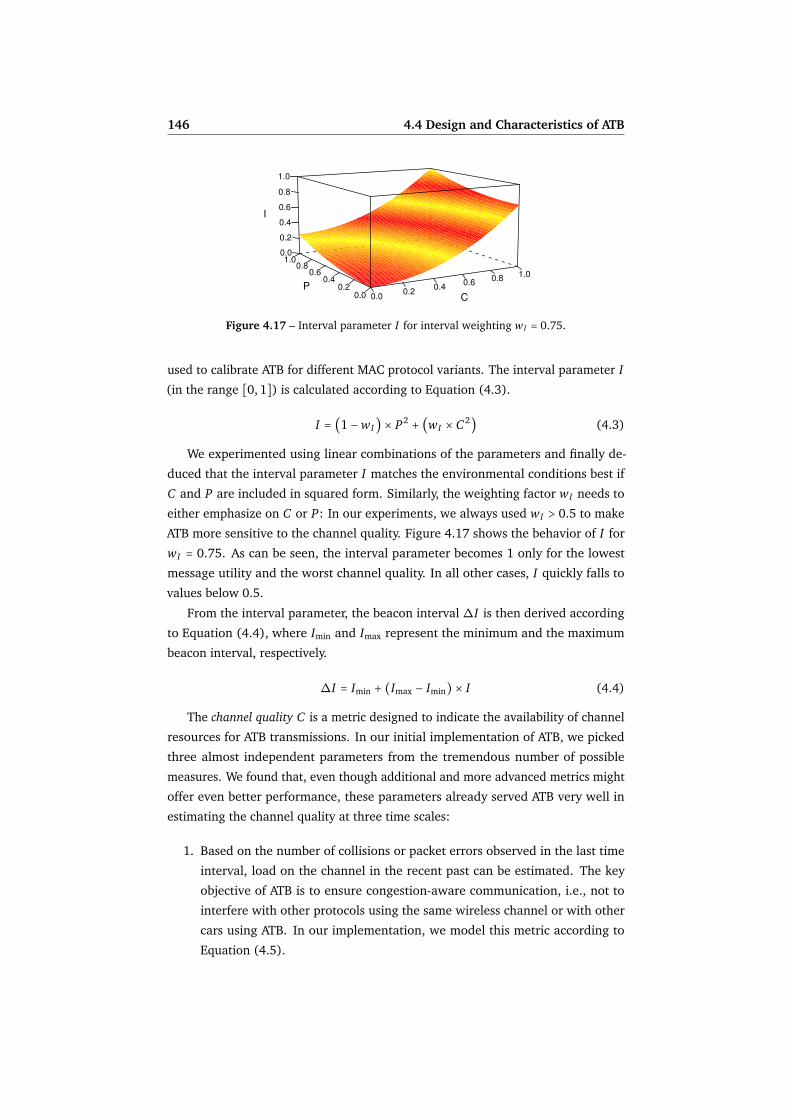
146 4.4 Design and Characteristics of ATB
0.00.2
0.40.6
0.81.0
0.00.2
0.40.6
0.81.0
0.0
0.2
0.4
0.6
0.8
1.0
C
P
I
Figure 4.17 – Interval parameter I for interval weighting wI = 0.75.
used to calibrate ATB for different MAC protocol variants. The interval parameter I
(in the range [0, 1]) is calculated according to Equation (4.3).
I = (1 − wI) × P2 + (wI × C2) (4.3)
We experimented using linear combinations of the parameters and finally de-
duced that the interval parameter I matches the environmental conditions best if
C and P are included in squared form. Similarly, the weighting factor wI needs to
either emphasize on C or P: In our experiments, we always used wI > 0.5 to make
ATB more sensitive to the channel quality. Figure 4.17 shows the behavior of I for
wI = 0.75. As can be seen, the interval parameter becomes 1 only for the lowest
message utility and the worst channel quality. In all other cases, I quickly falls to
values below 0.5.
From the interval parameter, the beacon interval ∆I is then derived according
to Equation (4.4), where Imin and Imax represent the minimum and the maximum
beacon interval, respectively.
∆I = Imin + (Imax − Imin) × I (4.4)
The channel quality C is a metric designed to indicate the availability of channel
resources for ATB transmissions. In our initial implementation of ATB, we picked
three almost independent parameters from the tremendous number of possible
measures. We found that, even though additional and more advanced metrics might
offer even better performance, these parameters already served ATB very well in
estimating the channel quality at three time scales:
1. Based on the number of collisions or packet errors observed in the last time
interval, load on the channel in the recent past can be estimated. The key
objective of ATB is to ensure congestion-aware communication, i.e., not to
interfere with other protocols using the same wireless channel or with other
cars using ATB. In our implementation, we model this metric according to
Equation (4.5).

4.4 Design and Characteristics of ATB 147
2. An estimate for the current transmission quality is the SNR as perceived
for the last transmission. In measurements, it has been shown that the
error rate of WiFi communication quickly increases if the SNR drops below
25 dB [135]. Therefore, we model this metric according to Equation (4.6),
with SNRmax = 50 dB, so that the metric already decreases to 0.25 for an SNR
equal to 25 dB.
3. We need to predict the probability of other transmissions in the next time
interval. Here, we use the density of vehicles (i.e., the number of neighbors)
to estimate the congestion probability (the more neighbors, the higher the
probability for simultaneous transmissions). We model this metric according
to Equation (4.7).
Finally, the channel quality C can be calculated according to Equation (4.8),
where the factor wC ≥ 1 is used to weight the measured parameters K and S higher
than the estimated congestion probability N .
K = 1 − 11 +#collisions
(4.5)
S = max⎧⎪⎪⎨⎪⎪⎩
0; ( SNRSNRmax
)2⎫⎪⎪⎬⎪⎪⎭
(4.6)
N = min⎧⎪⎪⎨⎪⎪⎩( #neighbors
#neighborsmax)
2
; 1⎫⎪⎪⎬⎪⎪⎭
(4.7)
C =N + wC × S+K
2
1 + wC(4.8)
The message utility P is an indicator for the demand to broadcast messages early
and frequently. Basically, the message utility allows nodes to schedule the next
transmission in a way that nodes having high priority messages will be able to
transmit first.
In our initial implementation of ATB, we calculate the message utility P as a
function of the age of the TIS data, the distance to the event source, the distance to
the next RSU, and how well the information is already disseminated. The message
utility is calculated for the TIS data with the highest utility in the local knowledge
base (see Section 4.4.4).
1. First, information age is accounted for by weighting it with the maximum
beacon interval Imax according to Equation (4.9). The older the information is,
the less frequently it should be distributed (bounded by the maximum beacon
interval Imax).

148 4.4 Design and Characteristics of ATB
2. The next two metrics to be considered represent the node’s proximity to
the event according to Equation (4.10) as well as its proximity to the next
RSU Equation (4.11). Both metrics take the current speed v of the vehicle
into account to measure proximity in the form of an estimated travel time.
This distance estimation can be further enhanced using map and location
information as described in the TO-GO approach [98].
3. Finally, the message utility is scaled based on how well its contents are already
disseminated. This measure, which is only used if the last beacon was received
from an RSU, ensures that messages are quickly forwarded to the local RSU if
it lacks information carried by the vehicle. Taking into account how much of
the information to be sent was not received via an RSU, this factor is calculated
according to Equation (4.12).
The message utility P can then be calculated according to Equation (4.13).
A = min⎧⎪⎪⎨⎪⎪⎩(message age
Imax)
2
; 1⎫⎪⎪⎬⎪⎪⎭
(4.9)
De = min⎧⎪⎪⎨⎪⎪⎩(distance to event / v
Imax)
2
; 1⎫⎪⎪⎬⎪⎪⎭
(4.10)
Dr = max⎧⎪⎪⎨⎪⎪⎩
0; 1 −√
distance to RSU / vImax
⎫⎪⎪⎬⎪⎪⎭(4.11)
B = 11 +#unknown entries
(4.12)
P = B × A+ De + Dr
3(4.13)
4.4.3 Flexible Use of Infrastructure Elements
ATB has been designed keeping in mind the possible exploitation of available infras-
tructure elements. Thus, deployed RSUs and even Traffic Information Centers (TICs)
are inherently supported by ATB.
In principle, ATB-enabled vehicles and ATB-enabled RSUs operate in a similar
fashion. RSUs participate in the beaconing process and adapt the beacon interval
according to the same rules described in Section 4.4.2. Thus, an RSU can simply be
deployed as a standalone system, e.g., with an attached solar cell for autonomous
operation. This is similar to the concept of stationary support units [102].
As shown in Figure 4.16, the RSUs can also be connected to a backbone network.
This connection is used by ATB to inform other RSUs about received traffic informa-
tion. In turn, the other RSUs update their local knowledge base accordingly, using
the same procedure as when receiving a regular beacon. We further assume that

4.4 Design and Characteristics of ATB 149
these RSUs also know their geographic position and the positions of the neighboring
RSUs. Therefore, data muling concepts as described in [149] can be realized.
The main difference between RSUs and vehicles is the calculation of the beacon
interval. RSUs are not able to estimate their travel time to a traffic congestion. Thus,
these metrics are ignored resulting in slightly shorter beacon intervals, according to
Equations (4.14) and (4.15).
PRSU = B × A (4.14)
IRSU = (1 − wI) × PRSU + (wI × C) (4.15)
Last but not least, the RSUs can be connected to one or more central TICs. A TIC
disseminates received TIS data differently than the vehicles and RSUs. Using the
available topology information of the connected RSUs, only relevant (i.e., geograph-
ically related) information is transmitted to each RSU. We modeled this mechanism
by defining a circular area for the RSUs within which information is considered
relevant.
4.4.4 TIS Data Management
The concept of ATB is to maintain local knowledge bases that contain all received
traffic information in aggregated form. In order to maintain the scalability of the
TIS, the transmission of irrelevant information needs to be suppressed and each
knowledge base needs to contain all received traffic information in a coarsely-
grained, aggregated form [142].
The operation of ATB, however, is independent from the scheme used for the
selection of knowledge base entries and their aggregation, so any of the numerous
approaches in the relevant literature can be used in an implementation.
An elaborate treatment of these topics, along with a probabilistic aggregation
scheme for message store maintenance, can be found in literature [101] and even
more advanced schemes, which could potentially support the assembly of multiple
beacon messages for parallel transmission over multiple channels, certainly warrant
further investigation.
As a baseline for our evaluation of the message dissemination characteristics,
however, we implemented a simplistic scheme: Our initial implementation of ATB
simply stores only the most recent information for each route segment, i.e., new
information elements either update records for an existing route segment (either
in part or as a whole) or they are appended to the knowledge base. In order to
deliver better performance and scalability, it can, however, be readily extended
to employ advanced data management and aggregation techniques found in the
literature [98,102,195].

150 4.4 Design and Characteristics of ATB
IDLE
In knowledge base?
Received Beacon
NO
YES
Extract next Entry
Insert Entry Merge Entry
More entries available?
NO
YES
Update entry priorities
Sort entries
Send Beacon
I = f(P, C)
Prune entries
Waiting time ≥ I
Figure 4.18 – Core functionality of the ATB protocol. Vehicles update a localknowledge base with entries from received beacons. The interval betweenbeacons is continuously adjusted based on P and C .
In our implementation, illustrated in Figure 4.18, the knowledge base is up-
dated with every received beacon, each of which may contain multiple information
elements. We prioritize entries to be transmitted in a beacon according to their
age δtentry = t − tentry, the proximity to the event tc = distance to event / v and the
proximity to the next RSU t r = distance to RSU / v. Based on these measures, the
priority of each entry can be calculated according to Equation (4.16).
pentry = δtentry − tc + t r (4.16)
Using the calculated priorities, beacon messages can be generated by selecting
as many entries as there is room in a single IEEE 802.11p frame [67] from the top
of the list, i.e., those with highest priority.
A single entry in a beacon comprises at least the following elements: Event type,
time, position, priority, and RSU identifier. Thus, after receiving a beacon, each of
its entries can simply be compared with the local knowledge base. If the event is
not yet known, the entry is appended. Otherwise it is updated appropriately. Each
update results in the re-calculation of the priorities of all entries and the calculation
of the next beacon interval.

4.4 Design and Characteristics of ATB 151
4.4.5 Security and Privacy Issues
ATB does not include specific security measures. Nonetheless, as discussed in [82],beaconing can be adequately secured using signatures and certificates added to
appropriately selected messages, e.g., with the help of Wireless Access in Vehicular
Environments (WAVE) security services [183]. In general, the computational and
the protocol overhead for this is not negligible, but this data can be omitted, e.g., if
transmitting multiple beacons among the same stations [82].Also highly relevant are questions surrounding privacy issues [46, 123]. The
transmitted TIS data, however, does not contain the ID of any vehicle. The only
identifier used in the traffic information is that of used RSUs, which we assume
does not raise specific privacy concerns. Therefore, aside from potential revealing
properties of the knowledge base entries transmitted, which certainly warrant further
exploration, the operation of ATB does not further interfere with privacy enhancing
schemes implemented on lower protocol layers.
4.4.6 Behavior on a Microscopic Level
As the behavior of ATB on the system level is dictated by the local behavior of
individual nodes, we first illustrate how ATB behaves on the microscopic level by
means of a simple example. Assume that ATB is deployed in the scenario shown
in Figure 4.19. At the beginning of the observed time interval, car A senses a new
event, which it will distribute to the nearby cars B, C, D, and E. Suppose some time
later, car F, which is just out of range of car A, will sense a new event, too, which it
will proceed to distribute. Drawn in the style of a timing diagram the figure gives an
example of how this scenario might play out. Please note that small values for C and
P denote a free channel and a high message utility, respectively. From top to bottom,
we plot the following four metrics of ATB: first, the time when an entry is inserted
into a vehicle’s knowledge base, i.e., the time when a new event was created (cars A
and F) or when a broadcast was received (cars B, C, D, and E). Secondly, we plot
the values of the message utility metric P and the channel quality metric C , which
are used by ATB to calculate the beacon interval. Lastly, we indicate the time when
an event is broadcast on the channel.
As can be observed, car A registers the new event at maximum values of both
message utility P and channel quality C . Car A therefore chooses its minimum
beacon interval for its next transmission, broadcasting the event almost immediately.
For the sake of example, we assume that car B is the first vehicle to process the
reception of this broadcast (taking operating system and other issues into account),
i.e., it becomes ready to re-broadcast first, followed shortly by car C. Thus, car B
is free to transmit its next beacon instantly – unlike car C, which observes these
two broadcasts within a short time interval and thus deduces a low value for the

152 4.4 Design and Characteristics of ATB
time
PC
bcas
t time
time
A B C ED F
A
B
C
E
D F
"unloaded"
"important"
"busy"
"less important"
Figure 4.19 – Behavior of ATB on a microscopic level, plotted in the style ofa timing diagram. One new event each is to be disseminated by car A, thencar F. Metrics P and C work in harmony to keep beacon frequency high, butchannel use low, allowing car F to instantly broadcast.
channel quality metric C . Following the presented algorithm, it reacts by increasing
its beacon interval, postponing its broadcasting of the event.
This broadcast, however, interferes with the desire of cars D and E to broadcast
the event themselves. Both cars now derive not only a low channel quality metric C ,
but (based on the increased event distance and age) also a lower message utility
metric P. This leads to them postponing their broadcast even further, leaving the
channel idle for now.
Thus, car F, which needs to disseminate a new event, is presented with ideal
channel conditions and, thus, arrives at a maximum value for the channel quality
metric C . Taken together with the message utility metric P, which assumes its
maximum value because of the event being new, this leads to car F choosing its
minimum value for the beacon interval. It can hence instantly broadcast a beacon
containing the new event. Of course, each message may include multiple events.
This example thus illustrates how the chosen metrics work in harmony to keep
nodes’ beacon frequency high whenever necessary, but the number of collisions on
the channel low, helping ATB adapt to highly dynamic network conditions – both
proactively and reactively. Moreover, even if adverse conditions lead to an erroneous
application of the heuristics used by ATB and, thus, to a disadvantageous beacon
interval being chosen for a transmission, the protocol is designed to quickly recover
from such states.

4.5 Performance Evaluation of ATB 153
(a) (b)
0 1km Copyright © 2008 OpenStreetMap (openstreetmap.org)This work is licensed under the CreativeCommons Attribution-ShareAlike 2.0 License.http://creativecommons.org/licenses/by-sa/2.0/
StartStart
IncidentIncident
FinishFinish
(c)
Figure 4.20 – Scenarios used for the performance evaluation: (a) a simpledetour, (b) a grid-shaped road network of 5 km and 16 km width, (c) a smallsection of the road network in Erlangen.
4.5 Performance Evaluation of ATB
We evaluated ATB in several simulation experiments to investigate the influence
of different protocol parameters, to compare it with traditional approaches, and
to show the feasibility in a real-world scenario. In the following, we describe the
experiments and discuss the results of the evaluations.
4.5.1 Simulation Environment and Parameters
We investigated the performance of ATB with the help of our Veins simulation
environment (presented in detail in Section 3.1), in which we configured three
classes of settings, as illustrated in Figure 4.20. For each part of the analysis, we
used an appropriate simulation scenario in order to clearly show the specific protocol
characteristics.
The knowledge base of ATB-equipped vehicles is checked after processing each
received beacon to identify events on the current route of the vehicle. If an incident
is found, an alternative route is calculated using the Dijkstra shortest path algorithm.
Similarly, resolved traffic congestions trigger a re-calculation of the route to check
whether there is now a shorter route to the destination.
We modeled vehicles capable of exchanging information using ATB by imple-
menting the protocol in Veins according to the principles described in Section 4.4.
ATB data was encapsulated in UDP/IP packets and sent on the channel via broadcast
messages. The radio channel and an IEEE 802.11b NIC transmitting at 11 Mbit/swas modeled by the INET Framework.

154 4.5 Performance Evaluation of ATB
Parameter Value
minimum beacon interval Imin 30 msmaximum beacon interval Imax 60 schannel quality weighting wC 2interval weighting wI 0.75number of neighbors for N = 1 50SNR for S = 1 50 dBneighborship data expiry 60 sTIS data expiry tstore 120 sreport traffic incident after queuing 10 sTIC radius of interest 5 kmprocessing delay 1 ms . . . 10 mschannel bitrate 11 Mbit/sapprox. transmission radius (Friis) 180 m
vehicle mobility model Kraußmax. speed 14 m/smax. acceleration 2.6 m/s2
dawdle time 0.5 smax. deceleration 4.5 m/s2
vehicle length 5 m
Table 4.6 – Simulation parameters modeling ATB-enabled nodes.
Vehicles moved with a maximum speed of 14 m/s (50.4 km/h, 31.32 mph) and
according to the Krauß mobility model. Timeout values used for TIS data expiry
were selected according to the accident lengths used in the simulations. The full set
of simulation parameters common to all scenarios can be found in Table 4.6.
For each scenario, we performed multiple simulation runs for statistical validity
and to identify outliers, but no less than 10 runs, and assessed the impact of TIS
operation using two primary performance metrics.
First, we tracked the effective average speed of vehicles, i.e., the time it takes a
vehicle to reach its destination in relation to the traveling time on the shortest route.
This metric reflects the benefit of the TIS on traffic as a whole.
Its impact on individual vehicles, smoothing the traffic flow, is reflected in a
second metric, the amount of emitted CO2. For calculating the CO2 emissions we
employ our implementation of the EMIT emission model (cf. Section 3.2).
4.5.2 Evaluation of Adaptivity
In a first set of simulations based on an initial implementation [94] of ATB, we
evaluate the presented metrics and their impact on adaptivity to rapid changes
in network conditions. We base this evaluation on a synthetic rear-end collision
scenario in order to provide a challenging, highly dynamic environment.

4.5 Performance Evaluation of ATB 155
We set up traffic on the simple single-lane road network shown in Figure 4.20a,
which consists of a 300 m main road and a 350 m detour. Traveling along the main
road are 101 cars, one departing every 5 s. The first vehicle is configured to stop
from t = 45 s . . . 105 s, near the end of the main road, creating an artificial traffic
incident.
All vehicles use ATB to exchange information about obstructions, the parameters
of ATB being configured as follows: minimum and maximum beacon interval are set
to Imin = 30 ms and Imax = 60 s, the weighting wI of channel quality set to 0.75, the
relative weight of K and S vs. N to 2. Vehicles generate a traffic incident event after
being blocked for 10 s and set its validity to 120 s.
During the course of this scenario, we record the two compound metrics that
ATB uses to adapt the beacon interval (message utility P and channel quality C)
along with their feedback on K. Thus we are able to investigate the frequency of
collisions on the channel and, hence, the degree to which ATB adapts to changing
network conditions.
We present the values of these metrics in the form of scatter plots, derived from
an exemplary simulation run. For ease of reference, observations are plotted in red
or blue, depending on whether they are recorded before or after the traffic incident
is cleared. In order to give an indication of message frequency, each individual
observation of P and C is plotted with low opacity, so a larger number of similar
observations results in a more pronounced dot. Values of the collision metric K are
always plotted at full opacity, so that individual outliers are distinctly visible in the
figure.
As shown in Figure 4.21, the first message informing vehicles of the incident
ahead can be observed at t = 55 s. Message utility P and channel quality C are at
their maximum values, as both the distance to and the age of the event are minimal
and the channel is unused. Both P and C thus allow the event to be disseminated
among nearby vehicles at a very high rate, as evidenced by the large number of
observations in the first few seconds. This, however, causes channel use to spike
and, consequently, the channel quality metric C of nearby nodes to drop by as much
as 10 % within fractions of a second.
Owing to the combined use of channel quality C and message utility P for the
calculation of I , however, the impact of this change on message frequencies is
immediate, as ATB adapts the beacon interval of nodes to match the deteriorating
channel. Thus, the number of collisions can be seen to remain negligible while
information about the incident is being disseminated at the maximum affordable
rate. Over the next seconds, the message utility P continuously decreases with
increasing age of the event, reflecting its decreased urgency, leading to a decrease
in overall beacon frequency and, thus, a very lightly loaded channel.

156 4.5 Performance Evaluation of ATB
(a) message utility metric P
(b) channel quality metric C; inset: collision metric K
Figure 4.21 – Changes in the metrics ATB uses to adapt the beacon intervalduring the synthetic rear-end collision scenario, both before (red) and after(blue) the incident is cleared. P and C are normalized from -1 (worst) to 0(best).
At t = 105 s, the artificial incident is cleared and, thus, a new event needs to
be disseminated in the now very crowded area around the point of origin. Mes-
sage utility P of the new event starts out at its maximum value to promote quick
dissemination of the event in the network.
If this metric was used alone, an incommensurate increase in channel load
would now be triggered, as this time node densities in the vicinity of the incident
are substantially higher. However, as the number of neighbors is factored into C ,
the high values of P are compensated for in the calculation of I and no substantial
increase in collisions on the channel can be observed. Thus, the chosen metrics
work in harmony to help ATB adapt to highly dynamic network conditions both
proactively and reactively.

4.5 Performance Evaluation of ATB 157
4.5.3 Comparative Evaluation
In order to evaluate the performance of ATB in terms of its impact on road traffic,
we rely on scenarios used in the literature [170]. As illustrated in Figure 4.20b, two
grid-shaped road networks of 5 km and 16 km width were prepared with horizontal
and vertical roads spaced 1 km apart. Starting in one corner, vehicles can then use
dynamic routing to avoid obstructions on their way to the opposite corner.
In a first set of simulation runs, we configured 30 vehicles to drive on the 5 km2
grid, one departing every 4 s. An artificial traffic incident is created by stopping
the lead vehicle for 60 s. We used this scenario to compare the performance of
ATB in three network configurations. One offers no infrastructural support, one
supports TIS operation by a network of RSUs spread over the intersections, and
one contains an additional TIC connected to the network. In order to compare the
performance of ATB with that of a protocol based on fixed beacon intervals, we also
simulated configurations of ATB using Imin = Imax. The resulting fixed beaconing
scheme, however, still includes our optimizations to start beaconing only if data
is available. Furthermore, we simulated two baseline scenarios without any radio
communications, one with and one without the artificial traffic incident.
Box plots from this set of simulation runs are shown in Figure 4.22. Dotted lines
mark the best and worst cases observed in the baseline scenarios. Aside from the
obvious improvements that ATB demonstrates, two common effects can be observed
from the evaluation: enabling Car-to-X capabilities of simulated vehicles leads to
some of them reaching their destination even faster than the fastest vehicles in an
obstruction-free scenario. This is because re-routing around the obstruction leads to
traffic flows being more evenly distributed over the network, avoiding micro-jams at
corners or intersections [162]. Yet, warning some vehicles too late, but also too early,
causes them to take unnecessary detours, which results in some vehicles arriving at
their destination later than they would have when sticking to their original route.
Still, the use of ATB, in particular when supported by infrastructure, typically leads
both to lower emissions and to vehicles reaching their destination faster than is
possible using fixed beacon intervals, even as short as 1 s.
In a second set of simulation runs, we therefore examined how ATB performs
when compared with beacon protocols using even shorter fixed beacon intervals.
We also increased the size of the road grid to 16 km2 and the number of cars to 1000
to obtain meaningful results for message delays.
We first examined the impact of TIS operation on vehicles’ speeds and CO2 emis-
sions for fixed beacon intervals and for ATB. The results are plotted in Figure 4.23a,
which shows the metrics’ mean values as well as the 10 % and 90 % quantile. As can
be seen it is not until beacon intervals of 1 s are used that results become comparable
with those of ATB.

158 4.5 Performance Evaluation of ATB
free none 10s 1s ATB /RSU /TIC
10
11
12
13
14
Effective a
vg. speed in m
/s
(a) effective average speed
free none 10s 1s ATB /RSU /TIC
11
00
11
50
12
00
12
50
13
00
CO
2 e
mis
sio
n in
g
(b) CO2 emission
Figure 4.22 – Effective average speed of vehicles and their CO2 emissionsin the 5 km2 grid setup. Plotted are two baseline settings, fixed intervalbeaconing, and ATB with three levels of infrastructure support.
We further examined this scenario by comparing for the same setups the end
to end delays of generated traffic information. Figure 4.23b shows this metric in
the form of empirical CDF plots. As can be seen, ATB performance can just match
that of fixed beaconing with intervals. The depicted delays represent the typical
store-carry-forward behavior in vehicular networks, which is greatly influenced by
the mobility of vehicles. It also needs to be mentioned that the absolute measures
need to be carefully evaluated because lost messages do not contribute to the CDF.
From these results, we see that static beaconing with a period of well under 1 s
allows for a similar range and quality of the TIS information exchange. However,
as can be seen from Figure 4.23c which depicts the number of collisions observed
on the channel per packet received in a log-scale graph, the load caused by the
static beaconing increases exponentially for smaller periods. In contrast, ATB is able
to perform well in all the investigated scenarios. Thus, we can conclude that ATB
succeeds at managing access to the radio channel – which, according to the used
quality metrics, also holds if other devices or applications start sharing the same
wireless channel.

4.5 Performance Evaluation of ATB 159
12.7
512.8
512.9
5
Avera
ge s
peed in m
/s
10s 3s 1s 300ms 100ms 30ms ATB
4880
4940
CO
2 in g
Beacon interval
(a) traffic performance
0 20 40 60 80 100
0.0
0.2
0.4
0.6
0.8
1.0
end to end delay in s
CD
F
100 ms
1 s
10 s
ATB
(b) empirical CDF of end to end delay
10s 3s 1s 300ms 100ms 30ms ATB
0.1
1.0
10.0
100.0
1000.0
Beacon interval
MA
C la
yer
colli
sions
obse
rved
(c) MAC layer collisions
10s 3s 1s 300ms 100ms 30ms ATB
10
20
30
40
50
60
Beacon interval
Em
erg
ency m
sg d
ela
y in s
priority 2
priority 10
(d) mean delay of a high-priority message
Figure 4.23 – TIS performance metrics recorded in the 16 km2 grid scenariofor various fixed beacon intervals as well as for ATB.

160 4.5 Performance Evaluation of ATB
As an example, we introduce into the TIS an emergency message to be dis-
seminated by the 101st vehicle at the same time that the first incident is reported,
then recording the mean delay the message experiences on its way through the
network. We configure the relative utility of the message as either 10× or 2× that of
a comparable regular TIS message, both in terms of P and pentry.
The results of this evaluation of simple application multiplexing on ATB are
plotted in Figure 4.23d. Results indicate that ATB was able to transmit an emergency
message even faster than was possible using a fixed beacon interval of 30 ms, the
minimum beacon interval of ATB in our setup.
4.5.4 Realistic City Scenario
In order to evaluate the performance of ATB in a less synthetic scenario, we chose a
road network based on OpenStreetMap data of the city of Erlangen. The modeled
section of the city comprises the university campus and a business park about 5 km
away. Both are connected by two trunk roads, but are reachable also via several
residential roads, as illustrated in Figure 4.20c. On this network, we configure a flow
of 200 vehicles, one departing from the university campus every 6 s and heading to
the business park. We introduce a traffic obstruction by stopping the lead vehicle for
240 s as it passes a short one-lane section in the road network. All vehicles following
the lead vehicle are therefore either caught in the jam, or, if informed early enough,
are able turn back and pick an alternate route.
Shown in Figure 4.24a are the results gathered from this series of simulations,
plotting in the style of a scatter plot for one exemplary run the effective average
speed and the CO2 emission of each vehicle vs. its time of departure. Again we plot
results for unobstructed traffic, no Car-to-X communication capabilities, for fixed
beacon intervals of 10 s and 1 s length, and for ATB.
As can be seen from the plot, the traffic obstruction substantially delays all
vehicles caught in the jam. Only vehicles departing later than just over 400 s enter
the simulation late enough to be uninfluenced by the 240 s incident. Both the
protocols using a fixed beacon interval and ATB again manage to inform most
vehicles of the obstruction in time. Also visible is a group of vehicles that can simply
not avoid the incident because they are already driving on the single-lane road
segment, as well as a group of vehicles that can avoid the incident, but have to turn
around to do so. Only at one point in the simulation, when the artificial jam begins
to dissolve, a fixed beacon interval of 10 s proves too coarse to keep some vehicles
from immediately entering the area of the jam.
No secondary jams could be observed in this scenario. The traffic density in
this scenario was low enough that all vehicles can be accommodated by the various
detours and continue to their destination unobstructed. In a second set of simulation

4.5 Performance Evaluation of ATB 161
Effective a
vg. speed in m
/s
810
12
free
none
10s
1s
ATB
0 100 200 300 400 500 600
Vehicle Departure Time in seconds
CO
2 in g
900
1100
(a) default scenario
Effective a
vg. speed in m
/s
810
12
free
none
10s
1s
ATB
0 100 200 300 400 500 600
Vehicle Departure Time in seconds
CO
2 in g
900
1100
(b) additional vehicle flow saturating detours
Figure 4.24 – Traffic performance in Erlangen scenarios.
Min. 1st Qu. Median Mean 3rd Qu. Max.
default 0.03 0.05 0.06 1.20 0.14 15.55two flows 0.03 0.06 0.10 3.72 5.39 16.02
Table 4.7 – Beacon intervals selected by ATB in the Erlangen scenarios (in s).
runs, we therefore set up an additional flow of vehicles which saturates the region
crossed by popular detours, indicated by a red, dashed arrow in Figure 4.20c.
Results gathered from this series of simulations, restricted to those gathered from
vehicles of the original traffic flow, are shown in Figure 4.24b. As the additional
flow of vehicles leads to the detours quickly becoming congested, this scenario
contains numerous secondary jams which require continuous re-routing of vehicles.
Again ATB manages traffic flows very well despite the large number of concurrent
messages. Still, a fixed beacon interval of 1 s can be seen to improve overall traffic
performance slightly beyond the capabilities of ATB. The reason for this behavior,
however, is illustrated in Table 4.7: In order to avoid collisions on the radio channel,
ATB has to operate with a much higher mean beacon interval of 3.72 s.


4.6 Comparison of ATB with Flooding/DTN 163
4.6 Comparison of ATB with Flooding/DTN
We now evaluate the performance of ATB in terms of dissemination speed, the classic
domain of flooding-based schemes. We compare the performance of ATB with that
of the most closely related and most recent of these schemes, DV-CAST, which – as
was presented in Section 2.4.2 – operates in a fully distributed manner, can keep the
network load within reasonable bounds, and is resilient to network disconnections.
Even though the concept of DV-CAST was developed for highway scenarios, its
flooding algorithm makes no assumptions about underlying road topology, and,
hence, can be deployed in any traffic scenario. In particular, DV-CAST incorporates
most recent findings on flooding approaches in dense scenarios to eliminate the
broadcast storm problem, and switches to a DTN approach in sparse scenarios.
Thanks to a close collaboration with the authors of DV-CAST [179], we were
able to successfully implement the protocol in the context of our Veins simulation
framework, calibrating protocol behavior to that of its original ns-2 model.
The scenario we use for this evaluation simulates traffic of varying density,
from 14 to 170 vehicles per km2, in the city of Ingolstadt, collating data points
from up to 100 independent runs to ensure the statistical significance of results.
The road network was based on the comprehensive road topology and attribute
database available from the OpenStreetMap project and adapted to reflect realistic
intersection management and timing. Traffic was generated by randomly selecting
source-destination pairs and iteratively applying the Dynamic User Assignment
(DUA) algorithm [54] until it reported a stable, optimal distribution of flows.
In the evaluation, we focus on the 4 km2 Region of Interest (ROI) shown in
Figure 4.25, which contains a heterogeneous mixture of high- and low-capacity
roads, traffic lights and unregulated intersections, as well as high- and low-density
areas. While traffic is simulated in the whole city of Ingolstadt to avoid border effects,
only vehicles within the ROI are considered to be participating in the network. In
order to determine how realistic this generated road traffic was, we implemented
induction loops in the ROI and compared the measured values with real values
provided courtesy of the local authorities. We observed that the range of traffic
densities spans from off-peak densities, e.g., the beginning of the morning rush hour
at 6:00 a.m., all the way down to sparse traffic at low equipment rates.
We use the same setup of ATB to enable the dissemination of information
about obstructions among vehicles. We evaluate the message dissemination speed
by triggering the transmission of a warning message at the intersection of the
two federal highways crossing this area, B 13 and B 16a (shown in dark red on
Figure 4.25). We keep track of whether each of the simulated cars received the
event and record its distance to the event’s origin for the duration of its validity.
This metric specifically includes cases where the event was not picked up by any

164 4.6 Comparison of ATB with Flooding/DTN
0 1 km
Figure 4.25 – Scenario used for the comparison to flooding: fully-detailed4 km2 section of Ingolstadt, containing a heterogeneous mixture of high- andlow-density areas, along with a crossing of two federal highways, B 13 andB 16a.
car. Moreover, it includes the progress of message dissemination achieved simply by
virtue of cars moving across the map.
As is common, we first examine the maximum distance covered by each message
as time progresses. Figure 4.26 illustrates how ATB compares to DV-CAST in this
respect, plotting the mean value of this distance for seven groups of the simulated
traffic densities. The interquartile range of results remained below 4 % at all times.
We observe that, in terms of dissemination speed, flooding clearly outperforms
our beaconing approach independent of the traffic density, having already bridged
several hundreds of meters before the first distance sample was taken. Yet, we also
observe that, due to the extremely high network dynamics in this scenario, the bea-
coning approach is more robust, leading to more widespread message propagation
in the long run. Nevertheless, it is not until several seconds after an event took place
that ATB reaches the same dissemination distance as DV-CAST.
However, we argue that examining the maximum dissemination distance alone
does not capture the benefit beaconing brings to frequently disconnected networks:
there is no clearly defined shock wave (the front of epidemically spreading infor-
mation) where all message transmissions take place, but rather a broad continuum

4.6 Comparison of ATB with Flooding/DTN 165
DV−CAST
ATB
1 2 5 10 20 50 100
05
00
10
00
15
00
time (in s)
max
. d
ista
nce (
in m
)
Figure 4.26 – Dissemination distance vs. time for 7 groups of traffic densitieswith means of 24, 51, 73, 98, 119, 151, and 170 vehicles per km2.
DV−CAST
ATB
0 500 1000 1500
0.0
0.2
0.4
0.6
0.8
1.0
distance (in m)
pen
etra
tio
n r
ate
Figure 4.27 – Dissemination quality vs. distance for 4 groups of traffic densi-ties with means of 19, 49, 97, and 159 vehicles per km2.
where nodes frequently exchange parts of their knowledge bases. This means
that disconnected clusters re-joining the network, even after several seconds of
disconnection, still have a very good chance of receiving and, in turn, being able to
disseminate these missed events.
We illustrate this in Figure 4.27, plotting for four groups of the simulated traffic
densities the ratio of nodes that received an event in a circular area centered on
its point of origin. The interquartile range of results remained below 5 % at all
times. We observe that, in particular at low densities and considering a large area
around the point of origin, adaptive beaconing achieves a noticeably higher event
penetration ratio, whereas flooding leaves large clusters of nodes unaware of an
event. However, we also observe how the lower speed of event dissemination of ATB
leads to its maximum of penetration ratios being shifted some hundreds of meters
away from the event source.


4.7 Conclusion 167
4.7 Conclusion
In this chapter we first presented the application of the presented simulative per-
formance evaluation techniques to protocol engineering, giving two examples of
distributed and centralized communication approaches, in short range WiFi and in
cellular networks.
Based on lessons learned, we then presented a new Car-to-X communication
protocol, Adaptive Traffic Beacon (ATB), which progresses beyond state-of-the-art
solutions by providing a self-organizing system architecture that automatically
adapts to various settings and conditions. ATB is based on a beaconing approach,
taking into account vehicle density, vehicles’ speed, radio communication reliability
and delay to optimize the beacon period. ATB is also adaptive in a second dimension.
It can automatically use optionally available infrastructure elements such as RSUs
or TIC servers. We evaluated the protocol performance in extensive simulation
experiments.
From the results, we conclude that ATB fulfills its task to support efficient TIS
data exchange with support for delay-sensitive and congestion-aware communica-
tion. ATB performs well in both synthetic scenarios and realistic urban networks,
without assuming the presence of (or creating and maintaining) network topology
or roadmap information.
Based on the comparison with a state-of-the-art hybrid flooding and DTN ap-
proach, we were able to further show that adaptive beaconing leads to a much
broader dissemination of messages, the predominant metric for non-safety appli-
cations. This distinction becomes even more pronounced in scenarios with low
traffic density or low equipment rates: here, the shock wave like dissemination of
messages in flooding based schemes simply skips temporarily-disconnected clusters.
On the other hand, flooding clearly outperforms beaconing in terms of dissemina-
tion speed, the predominant metric for safety applications. Adaptive beaconing and
flooding based schemes thus offer unique benefits and drawbacks, depending on
the envisioned application scenario.


Chapter 5
Conclusion
In the first part of this work, we demonstrated how to take the simulative per-
formance evaluation of Car-to-X communication systems one step beyond current
approaches: we presented our framework Veins for the co-simulation of commu-
nication networks and road traffic. Veins relies on a bidirectional coupling of
state-of-the-art simulators from both domains to incorporate well-known models for
road traffic microsimulation with a comprehensive selection of network protocol
models, and extends both for the evaluation of Car-to-X communication systems.
It allows simulating complex heterogeneous scenarios to a high degree of realism
and allows for road traffic to be influenced by network communication. Whenever
events in a network simulation can potentially affect the mobility of vehicles, any
approach based on trace data is unable to generate the required real-time interaction
between mobility model and application model. For the simulative performance
evaluation of such systems, e.g., for Traffic Information System (TIS) design, the
presented impact studies demonstrated not merely the applicability, but the outright
need for taking this approach.
We continued by describing how to employ the Veins simulation framework for
parameter studies and model validation and demonstrated the importance of con-
sidering metrics beyond isolated communication network and road traffic metrics by
highlighting cases where such metrics are conflicting. We presented a computation-
ally inexpensive model that, unlike traditional stochastic models, allows obtaining a
realistic estimate of predictable signal attenuation effects due to obstacles such as
buildings. We demonstrated the applicability of this model to simulate IEEE 802.11p
radio shadowing in urban and suburban environments based on extensive real-
world measurements. Based on the results of simulation studies performed with and
without this model, as well as real-world geodata with different levels of detail, we
concluded that including information beyond the mere topology of roads in Car-to-X
169

170 5 Conclusion
simulations can have a profound impact on core network metrics, both in terms of
aggregate statistics and shape of distribution.
We therefore argue that our approach constitutes a substantial contribution
to the methodology of simulative performance evaluation of Car-to-X systems; in
particular for studies that cannot afford to disregard microscopic network or radio
effects, as well for evaluations where Car-to-X communication would likely influence
driver behavior.
We decided to release our Veins simulation framework as Free and Open Source
Software, allowing anyone to freely inspect, use, adapt, and improve all of its
components. In order to coordinate efforts, we created a website12 to host the
framework and associated documentation, tutorials, and sample scenarios. Thus,
we are able to make available to interested researchers a freely available and openly
developed framework which offers the following features:
• it is based on Open Source software only, offering unrestricted extensibility,
• allows for online re-configuration and re-routing of vehicles in reaction to
network packets,
• relies on a trusted vehicular mobility model and implementation done by
Transportation and Traffic Science community,
• relies on fully-detailed models of network layers, including channel access,
noise and interference effects,
• can simulate city block level simulations in real time on a single workstation,
• can be deployed on compute clusters for simulation in an MRIP distributed
parallel fashion,
• can import whole scenarios from OpenStreetMap, including buildings, speed
limits, lane counts, traffic lights, access and turn restrictions,
• can employ a computationally inexpensive obstacle model of shadowing effects
caused by buildings,
• supplies data sources for a wide range of metrics, including travel time and
emissions,
• allows for the graphical, real time inspection of – and interaction with – both
the network and road traffic models, and
• is supported by a solid and diverse user base from five continents.
12http://veins.car2x.org/

5 Conclusion 171
In a second part of this work, we demonstrated how the presented approach
led us to the development of our Adaptive Traffic Beacon (ATB) protocol. We base
its design on lessons learned from evaluating common approaches to Car-to-X com-
munication systems, both infrastructure-based and infrastructure-less, identifying
adaptivity as the key property such approaches were lacking.
This led us to conceive ATB as an evolved beaconing approach designed for
operating in truly heterogeneous environments. One of the key goals of ATB is
to continuously adapt the interval between two beacons to utilize all unused ca-
pacity of the wireless channel, but never more. In this way, as far as high-priority
access to the medium is concerned, the channel appears virtually unloaded at all
times. Taken together, this enables ATB to support efficient TIS data exchange
in heterogeneous communication scenarios with support for delay-sensitive and
congestion-aware communication. Thus, ATB progresses beyond state-of-the-art
solutions by providing:
• a self-organizing system architecture, which
• keeps the channel virtually unloaded enabling high-priority access,
• allows for co-existence with other protocols and systems,
• is able to make use of optionally available infrastructure, and
• automatically and quickly adapts to changing network conditions.
We evaluated the performance of ATB with the help of the methodology we
presented in this work, as implemented in our Veins simulation framework. The
results of our in-depth studies validated both the core functionality and the adaptivity
of ATB to rapid changes in network conditions and presence of infrastructure. We
outlined the strengths of our adaptive beaconing approach in comparison to simpler,
non-adaptive protocols, both in synthetic and highly realistic scenarios.
Finally, we highlighted the strengths and weaknesses of ATB when compared
with state-of-the-art hybrid multi-hop flooding and disruption tolerant networking.
We were able to demonstrate that adaptive beaconing leads to a much broader
dissemination of messages, the predominant metric for non-safety applications. On
the other hand, flooding clearly outperforms beaconing in terms of dissemination
speed, the predominant metric for safety applications.
This means that flooding and disruption tolerant networking approaches fit the
requirements of safety applications very well. In contrast, the requirements of non-
safety applications in highly heterogeneous scenarios, in particular TIS, mandate a
novel approach to message dissemination, as represented by our ATB protocol.


List of Acronyms
3GPP Third Generation Partnership Project
AC Access Class
AIFS Arbitrary Inter-Frame Spacing
AODV Ad Hoc on Demand Distance Vector
ATB Adaptive Traffic Beacon
ATIS Alliance for Telecommunications Industry Solutions
BSS Basic Service Set
CALM Communications Access for Land mobiles
CCH Control Channel
CDF Cumulative Distribution Function
CDMA Code Division Multiple Access
CoCar Cooperative Cars
DCH Dedicated Channel
DHT Distributed Hash Table
DSDV Destination Sequenced Distance Vector
DSR Dynamic Source Routing
DSRC Dedicated Short Range Communications
DTN Delay/Disruption Tolerant Network
DYMO Dynamic MANET On Demand
EDCA Enhanced Distributed Channel Access
173

174 5 Conclusion
ETSI European Telecommunications Standards Institute
FACH Forward Access Channel
FDD Frequency Division Duplex
FTAP Fast Traffic Alert Protocol
GGSN Gateway GPRS Support Node
GPS Global Positioning System
HSPA High Speed Packet Access
IDM Intelligent-Driver Model
IETF Internet Engineering Task Force
ITS Intelligent Transportation Systems
IVC Inter-Vehicle Communication
MANET Mobile Ad Hoc Network
MBMS Multimedia Broadcast Multicast Service
MMS Multimedia Messaging Service
MOBIL Minimizing Overall Braking Induced by Lane-changes
MPI Message Passing Interface
MRIP Multiple Replications In Parallel
NHDP Neighborhood Discovery Protocol
OFDM Orthogonal Frequency Division Multiplexing
PDES Parallel Discrete Event Simulation
QoS Quality of Service
RACH Random Access Channel
RERR Route Error
RMSE Root Mean Square Error
ROI Region of Interest
RREP Route Reply

5 Conclusion 175
RREQ Route Request
RSU Roadside Unit
RSS Received Signal Strength
SCH Service Channel
SNR Signal to Noise Ratio
SOTIS Self-Organizing Traffic Information System
SUMO Simulation of Urban Mobility
TDD Time Division Duplex
TIC Traffic Information Center
TIS Traffic Information System
TPDP Traffic Probe Data Protocol
TPEG Transport Protocol Expert Group
TTL Time To Live
UMTS Universal Mobile Telecommunications System
UTRA Universal Terrestrial Radio Access
VANET Vehicular Ad Hoc Network
WAVE Wireless Access in Vehicular Environments
WBSS WAVE Basic Service Set
WSMP WAVE Short Message Protocol
WSN Wireless Sensor Network
ZRP Zone Routing Protocol


List of Figures
1.1 Concept of the 1983 Wolfsburger Welle demonstration project: in-
frastructure-to-car communication based on infrared transceivers is
employed to transmit traffic light phase information to oncoming
vehicles; source: [207]. . . . . . . . . . . . . . . . . . . . . . . . . . . 7
1.2 Highly dynamic, heterogeneous network conditions in an urban set-
ting: traffic alternates between free-flowing and queued conditions
(left) and vehicles frequently pass queued traffic at high speeds (right). 9
2.1 OMNeT++ hierarchical modeling paradigm. Shown is a simple mod-
ule connected via gates to a compound module; the latter contains
two more simple modules. . . . . . . . . . . . . . . . . . . . . . . . . . 18
2.2 Overview of the protocol layers covered by either the INET Framework
or the MiXiM module libraries for OMNeT++. . . . . . . . . . . . . . 20
2.3 Common convention of modeling in ns-2: shown is a typical configu-
ration of classifiers and connectors to form two nodes and a link. . . 22
2.4 Simple adaptations of the Random Waypoint mobility model as ap-
plied to vehicular movement. . . . . . . . . . . . . . . . . . . . . . . . 25
2.5 Screenshot of the optional graphical user interface to the SUMO
microscopic road traffic simulation environment. . . . . . . . . . . . . 30
2.6 OpenStreetMap web frontend showing a section of the city of Ingol-
stadt, Germany. . . . . . . . . . . . . . . . . . . . . . . . . . . . . . . . 32
2.7 Taxonomy of wireless communication technologies. . . . . . . . . . . 35
2.8 CALM architecture overview based on [73]. . . . . . . . . . . . . . . . 36
2.9 Overview of the WAVE stack and associated standards based on [78,
183]. . . . . . . . . . . . . . . . . . . . . . . . . . . . . . . . . . . . . . 37
2.10 Spectrum available in the U.S. DSRC band for use as Control Channel
(CCH) and general-purpose Service Channels (SCHs). Below: Current
and future spectrum allocated for ITS use in Europe and Japan; based
on [47,78]. . . . . . . . . . . . . . . . . . . . . . . . . . . . . . . . . . 38
177

178 List of Figures
2.11 Access procedure on the UMTS RACH: one failed, one successful
attempt [166]. . . . . . . . . . . . . . . . . . . . . . . . . . . . . . . . . 40
2.12 Taxonomy of IVC applications. . . . . . . . . . . . . . . . . . . . . . . 43
2.13 Routing information dissemination in AODV and DYMO. . . . . . . . 46
2.14 Concept of a simple flooding scheme for information dissemination in
MANETs. . . . . . . . . . . . . . . . . . . . . . . . . . . . . . . . . . . . 47
2.15 Impact of the broadcast storm problem on network performance;
based on results presented in a study of flooding on a 10 km four lane
highway reported in [177]. . . . . . . . . . . . . . . . . . . . . . . . . 47
2.16 Concept of a family of distance based schemes for broadcast suppression. 48
2.17 Message dissemination via beaconing, as envisioned in SOTIS. . . . . 50
2.18 On-the-fly generation of road maps for SOTIS. . . . . . . . . . . . . . 51
3.1 Mobility modeling techniques for simulation of IVC protocols and
applications. . . . . . . . . . . . . . . . . . . . . . . . . . . . . . . . . . 57
3.2 State machines of network and road traffic simulation frameworks’
coupling modules. . . . . . . . . . . . . . . . . . . . . . . . . . . . . . . 59
3.3 Sequence diagram of messages exchanged between network and
road traffic simulation frameworks’ coupling modules. Command
execution is delayed until the next road traffic simulation time step is
triggered. . . . . . . . . . . . . . . . . . . . . . . . . . . . . . . . . . . . 60
3.4 Screenshots of simulators’ graphical user interfaces running network
and road traffic simulations in parallel. . . . . . . . . . . . . . . . . . 62
3.5 Screenshot of the running simulative prototype. A contiguous stream
of vehicles, leaving the campus and heading to a business park, is
interrupted by a traffic obstruction at point ¬. Dynamic re-routing
has started. . . . . . . . . . . . . . . . . . . . . . . . . . . . . . . . . . . 63
3.6 Lifecycle management functionality of sumo-launchd. . . . . . . . . . 66
3.7 Baseline scenario used in the evaluation of performance metrics:
a single trunk road is connected to two slower parallel roads by a
number of rungs. Concept and representations in the network and
road traffic simulators. . . . . . . . . . . . . . . . . . . . . . . . . . . . 67
3.8 Impact of route choice on vehicle speed and acceleration profile. . . 71
3.9 Influence of stop time and rung length on travel time and CO2 emis-
sions; lead vehicle stops once. . . . . . . . . . . . . . . . . . . . . . . . 72
3.10 Influence of stop time on travel time and CO2 emissions; multiple stops. 72
3.11 Deterioration of RSS as a transmission is blocked by first one, then
two buildings. Input parameters of the presented model are the
buildings’ geometries and the positions of both the sending and the
receiving node. . . . . . . . . . . . . . . . . . . . . . . . . . . . . . . . 75

List of Figures 179
3.12 Position of the shark fin antenna assembly, omnidirectional antenna,
and GPS receiver used for signal attenuation measurements; inset:
installation of the DENSO WSU 802.11p radio in the trunk. . . . . . 79
3.13 Use of geodata on road network and building geometry in the data
correlation and verification step. Each line indicates one success-
ful transmission between sending and receiving car, a line’s color
representing the measured RSS value. . . . . . . . . . . . . . . . . . . 80
3.14 Attenuation values predicted by the empirical free space path loss
model (red circles) vs. measurement data in the unobstructed sce-
nario for a path loss exponent of α = 2.2. . . . . . . . . . . . . . . . . 81
3.15 Sharp drop and continuous decline in measured RSS as the length of
building penetrated increases. . . . . . . . . . . . . . . . . . . . . . . . 81
3.16 Comparisons of measured and calculated attenuation values for dif-
ferent types of buildings. . . . . . . . . . . . . . . . . . . . . . . . . . . 84
3.17 Screenshot of SUMO rendering part of the imported geodata on roads
and buildings in the city of Ingolstadt, as used in the full-featured
simulation scenario. . . . . . . . . . . . . . . . . . . . . . . . . . . . . . 89
3.18 Distribution of number of nodes in communication range. Shown are
results for radios of different power (results for a maximum range of
approx. 1.2 km are represented by the red, solid line) and map data
of different quality. Lower-quality map data can lead to unrealistically
dense car clusters. . . . . . . . . . . . . . . . . . . . . . . . . . . . . . . 91
3.19 Distribution of duration of contact with nodes in communication
range. Shown are results for radios of different power and map data
of different quality. Lower-quality map data can suggest overly long
and differently-distributed contact durations. . . . . . . . . . . . . . . 92
3.20 Map of Erlangen, Germany as available from the OpenStreetMap
project and used in the overall evaluation. Overlaid are the scenario’s
start and finish positions, the fastest route between them, and popular
alternative routes around the artificial incident. . . . . . . . . . . . . 93
3.21 Average speed of individual vehicles for free flowing traffic, traffic
with an incident, and when performing IVC. . . . . . . . . . . . . . . 95
3.22 Average CO2 emission of vehicles for free flowing traffic, traffic with
an incident, and when performing IVC. . . . . . . . . . . . . . . . . . 96
3.23 Heatmap of vehicle stop times in 25 m×25 m regions of the scenario.
Brighter shades of red indicate longer maximum stop times. . . . . . 97
3.24 Statistical analysis of driver behavior models. . . . . . . . . . . . . . . 100
3.25 Empirical CDF of the average speed achieved for the driver behavior
models. . . . . . . . . . . . . . . . . . . . . . . . . . . . . . . . . . . . . 101
3.26 Q-Q plot of probabilistic vs. mix driver behavior models. . . . . . . . 101

180 List of Figures
4.1 Screenshots of full-featured and minimal MANET nodes running
DYMO, as shown in OMNeT++. . . . . . . . . . . . . . . . . . . . . . 112
4.2 Exemplary results from the extensive performance evaluation study
of our DYMO model [153]. . . . . . . . . . . . . . . . . . . . . . . . . 113
4.3 The two types of IVC scenarios for which the performance of a de-
ployed MANET protocol was examined. . . . . . . . . . . . . . . . . . 115
4.4 Overview of the simulated grid scenario: single-lane roads are laid
out in a grid with a cell size of 1 km2. Start and finish node positions
are fixed. With no IVC, cars always pick the shortest route, illustrated
by the dotted line. . . . . . . . . . . . . . . . . . . . . . . . . . . . . . . 117
4.5 Average speed of individual vehicles, ordered by time of departure.
One scenario with free flowing traffic, one scenario with incident and
IVC. Vehicles poll the Traffic Information Center (TIC) every minute 119
4.6 Packet collisions on the wireless channel per packet sent. One sce-
nario with free flowing traffic, one with no IVC, four scenarios with
different types of VANET communication. . . . . . . . . . . . . . . . . 120
4.7 Vehicle speed averaged over all vehicles. One scenario with free
flowing traffic, one with no IVC, four scenarios with different types
of VANET communication. . . . . . . . . . . . . . . . . . . . . . . . . . 121
4.8 Component model of the simulated UMTS-based Car-to-X communi-
cation system. . . . . . . . . . . . . . . . . . . . . . . . . . . . . . . . . 123
4.9 OMNeT++ representation of a CoCar-enabled vehicle in UML notation.127
4.10 Empirical CDF of the random access procedure duration for the de-
fault set of parameters (c0=−6 dB, 2 dB power step, 1 RX antenna, 2
RACH subchannels), compared to alternative parameterizations. . . 130
4.11 Road map of the 10 km × 10 km simulation scenario and GUI screen-
shot of the traffic simulator, showing a subsection of the freeway
interchange during the simulation. . . . . . . . . . . . . . . . . . . . . 132
4.12 Impact of the CoCar communication system on road traffic: Quantiles
of vehicles’ CO2 emissions; empirical CDFs and median values. . . . . 135
4.13 Impact of the CoCar communication system on network traffic; em-
pirical CDFs and 90 % quantile. . . . . . . . . . . . . . . . . . . . . . . 136
4.14 End-to-end delay of CoCar messages, depending on the means of
delivery; empirical CDFs and 90 % quantile. . . . . . . . . . . . . . . . 138
4.15 Conceptual visualization of the beacon mechanism. Vehicles commu-
nicate by periodically exchanging parts of their knowledge bases. . . 141
4.16 ATB system architecture. . . . . . . . . . . . . . . . . . . . . . . . . . . 142
4.17 Interval parameter I for interval weighting wI = 0.75. . . . . . . . . . 146

List of Figures 181
4.18 Core functionality of the ATB protocol. Vehicles update a local knowl-
edge base with entries from received beacons. The interval between
beacons is continuously adjusted based on P and C . . . . . . . . . . . 150
4.19 Behavior of ATB on a microscopic level, plotted in the style of a timing
diagram. One new event each is to be disseminated by car A, then
car F. Metrics P and C work in harmony to keep beacon frequency
high, but channel use low, allowing car F to instantly broadcast. . . . 152
4.20 Scenarios used for the performance evaluation: (a) a simple detour,
(b) a grid-shaped road network of 5 km and 16 km width, (c) a small
section of the road network in Erlangen. . . . . . . . . . . . . . . . . . 153
4.21 Changes in the metrics ATB uses to adapt the beacon interval during
the synthetic rear-end collision scenario, both before (red) and after
(blue) the incident is cleared. P and C are normalized from -1 (worst)
to 0 (best). . . . . . . . . . . . . . . . . . . . . . . . . . . . . . . . . . . 156
4.22 Effective average speed of vehicles and their CO2 emissions in the
5 km2 grid setup. Plotted are two baseline settings, fixed interval
beaconing, and ATB with three levels of infrastructure support. . . . 158
4.23 TIS performance metrics recorded in the 16 km2 grid scenario for
various fixed beacon intervals as well as for ATB. . . . . . . . . . . . . 159
4.24 Traffic performance in Erlangen scenarios. . . . . . . . . . . . . . . . 161
4.25 Scenario used for the comparison to flooding: fully-detailed 4 km2
section of Ingolstadt, containing a heterogeneous mixture of high-
and low-density areas, along with a crossing of two federal highways,
B 13 and B 16a. . . . . . . . . . . . . . . . . . . . . . . . . . . . . . . . 164
4.26 Dissemination distance vs. time for 7 groups of traffic densities with
means of 24, 51, 73, 98, 119, 151, and 170 vehicles per km2. . . . . 165
4.27 Dissemination quality vs. distance for 4 groups of traffic densities
with means of 19, 49, 97, and 159 vehicles per km2. . . . . . . . . . . 165


List of Tables
2.1 Typical values of Krauß model parameters according to its original
publication [92]. . . . . . . . . . . . . . . . . . . . . . . . . . . . . . . 27
2.2 Typical values of IDM model parameters according to its original
publication [182]. . . . . . . . . . . . . . . . . . . . . . . . . . . . . . . 29
3.1 EMIT factors for the modeled class of vehicles. . . . . . . . . . . . . . 69
3.2 Simulation parameters used in the evaluation of performance metrics. 70
3.3 Investigated classes of driver behavior: four basic classes, three com-
bined classes. . . . . . . . . . . . . . . . . . . . . . . . . . . . . . . . . 99
3.4 Summary of related simulation tools [43]. . . . . . . . . . . . . . . . 104
4.1 Common parameters of a node running DYMO. . . . . . . . . . . . . 114
4.2 Road traffic microsimulation parameters modeling inner-city traffic
with somewhat inattentive drivers. . . . . . . . . . . . . . . . . . . . . 116
4.3 INET Framework module parameters modeling IVC-enabled vehicles. 117
4.4 Default set of parameters for the RACH. . . . . . . . . . . . . . . . . . 130
4.5 Road traffic microsimulation parameters modeling a mix of cars and
trucks. . . . . . . . . . . . . . . . . . . . . . . . . . . . . . . . . . . . . 133
4.6 Simulation parameters modeling ATB-enabled nodes. . . . . . . . . . 154
4.7 Beacon intervals selected by ATB in the Erlangen scenarios (in s). . . 161
183


List of Listings
2.1 Sample network description file for OMNeT++: two standard hosts
connected directly via Ethernet. . . . . . . . . . . . . . . . . . . . . . . 19
2.2 Sample simulation script for ns-2: two nodes running FTP over a TCP
connection. . . . . . . . . . . . . . . . . . . . . . . . . . . . . . . . . . . 21
2.3 Sample simulation script for ns-3 (adapted and shortened from docu-
mentation): two nodes send or receive UDP data. . . . . . . . . . . . 21
2.4 Sample OpenStreetMap XML data dump encoding information about
three nodes interconnected by a way. . . . . . . . . . . . . . . . . . . . 33
3.1 Excerpt of mobility data sent by an early version of the coupling
interface to the road traffic simulator. . . . . . . . . . . . . . . . . . . 61
3.2 Sample launch configuration for sumo-launchd. . . . . . . . . . . . . . 65
3.3 Sample edge definition file configuring default parameters for sec-
ondary roads. . . . . . . . . . . . . . . . . . . . . . . . . . . . . . . . . 88
3.4 Sample edge data in a SUMO road network data file. . . . . . . . . . 88
3.5 Sample polygon definition configuring import parameters for building
outlines. . . . . . . . . . . . . . . . . . . . . . . . . . . . . . . . . . . . 89
3.6 Sample polygon data in a SUMO supplementary data file. . . . . . . . 89
185


Bibliography
[1] 3GPP, “Physical layer procedures (FDD),” 3rd Generation Partnership Project
(3GPP), TS 25.214 v7.2.0, 2006.
[2] 3GPP, “User Equipment (UE) radio transmission and reception (FDD),” 3rd
Generation Partnership Project (3GPP), TS 25.101 v7.6.0, 2006.
[3] 3GPP, “Physical channels and mapping of transport channels onto physical
channels (FDD),” 3rd Generation Partnership Project (3GPP), TS 25.211
v7.3.0, 2008.
[4] S. AHMED, G. C. KARMAKAR, and J. KAMRUZZAMAN, “An Environment-Aware
Mobility Model for Wireless Ad Hoc Network,” Elsevier Computer Networks,
vol. 54, no. 9, pp. 1470–1489, May 2010.
[5] S. AHMED and S. S. KANHERE, “Cluster-based Forwarding in Delay Tolerant
Public Transport Networks,” in 32nd IEEE Conference on Local Computer
Networks (LCN 2007). Dublin, Ireland: IEEE, October 2007, pp. 625–634.
[6] K. AKKAYA and M. YOUNIS, “A Survey of Routing Protocols in Wireless Sensor
Networks,” Elsevier Ad Hoc Networks, vol. 3, no. 3, pp. 325–349, 2005.
[7] J. ALCARAZ, G. PEDRENO, F. CERDAN, and J. GARCIA-HARO, “Simulation of
3G DCHs Supporting TCP Traffic: Design, Experiments and Insights on
Parameter Tuning,” in 1st ACM/ICST International Conference on Simulation
Tools and Techniques for Communications, Networks and Systems (SIMUTools
2008): 1st ACM/ICST International Workshop on OMNeT++ (OMNeT++2008). Marseille, France: ACM, March 2008.
[8] M. ASEFI, J. MARK, and X. SHEN, “A Cross-Layer Path Selection Scheme for
Video Streaming over Vehicular Ad-Hoc Networks,” in 72nd IEEE Vehicular
Technology Conference (VTC2010-Fall). Ottawa: IEEE, September 2010.
[9] ASTM INTERNATIONAL, “ASTM E2213-03: Standard Specification for Telecom-
munications and Information Exchange Between Roadside and Vehicle Sys-
187

188 Bibliography
tems : 5 GHz Band Dedicated Short Range Communications (DSRC) Medium
Access Control (MAC) and Physical Layer (PHY) Specifications,” 2003.
[10] S. Y. BAEK, Y.-J. HONG, and D. K. SUNG, “Adaptive Transmission Scheme for
Mixed Multicast and Unicast Traffic in Cellular Systems,” IEEE Transactions
on Vehicular Technology, vol. 58, no. 6, pp. 2899–2908, July 2009.
[11] F. BAI and B. KRISHNAMACHARI, “Exploiting the Wisdom of the Crowd: Local-
ized, Distributed Information-Centric VANETs,” IEEE Communications Maga-
zine, vol. 48, no. 5, pp. 138–146, May 2010.
[12] W. BARFIELD, M. HASELKORN, J. SPYRIDAKIS, and L. CONQUEST, “Commuter
Behavior and Decision-Making: Designing Motorist. Information Systems,”
in 33rd Human Factors and Ergonomics Society Annual Meeting, Santa Monica,
CA, 1989, pp. 611–614.
[13] R. BARR, Z. J. HAAS, and R. VAN RENESSE, “JiST: Embedding Simulation Time
into a Virtual Machine,” in EuroSim Congress on Modelling and Simulation,
2004.
[14] D. M. BATES and D. G. WATTS, Nonlinear Regression Analysis and Its Applica-
tions. Wiley, August 1988.
[15] R. BAUZA, J. GOZALVEZ, and M. SEPULCRE, “Operation and Performance of
Vehicular Ad-Hoc Routing Protocols in Realistic Environments,” in 68th IEEE
Vehicular Technology Conference (VTC2008-Fall), Calgary, Alberta, Canada,
September 2008, pp. 1–5.
[16] N. BEL GEDDES, Magic Motorways. Random House, 1940.
[17] J. J. BLUM, A. ESKANDARIAN, and L. J. HOFFMAN, “Challenges of Intervehicle
Ad Hoc Networks,” IEEE Transactions on Intelligent Transportation Systems,
vol. 5, no. 4, pp. 347–351, December 2004.
[18] D. P. BOWYER, R. AKCELIK, and D. C. BIGGS, “Guide to fuel consumption
analysis for urban traffic management,” Australian Road Research Board,
ARRB Special Report 32, 1985.
[19] L. BRESLAU, D. ESTRIN, K. FALL, S. FLOYD, J. HEIDEMANN, A. HELMY, P. HUANG,
S. MCCANNE, K. VARADHAN, Y. XU, and H. YU, “Advances in network simula-
tion,” IEEE Computer, vol. 33, no. 5, pp. 59–67, May 2000.
[20] E. BROCKFELD and P. WAGNER, “Testing and Benchmarking of Microscopic Traf-
fic Flow Simulation Models,” in 10th World conference on transport research
(WCTR), Istanbul, Turkey, July 2004.

Bibliography 189
[21] T. CAMP, J. BOLENG, and V. DAVIES, “A Survey of Mobility Models for Ad Hoc
Network Research,” Wireless Communications and Mobile Computing, Special
Issue on Mobile Ad Hoc Networking: Research, Trends and Applications, vol. 2,
no. 5, pp. 483–502, 2002.
[22] A. CAPPIELLO, I. CHABINI, E. NAM, A. LUE, and M. ABOU ZEID, “A statistical
model of vehicle emissions and fuel consumption,” in 5th IEEE International
Conference on Intelligent Transportation Systems (IEEE ITSC), September 2002,
pp. 801–809.
[23] M. CATEDRA, J. PEREZ, F. SAEZ DE ADANA, and O. GUTIERREZ, “Efficient Ray-
Tracing Techniques for Three-Dimensional Analyses of Propagation in Mobile
Communications: Application to Picocell and Microcell Scenarios,” IEEE
Antennas and Propagation Magazine, vol. 40, no. 2, pp. 15–28, April 1998.
[24] I. CHAKERES and C. PERKINS, “Dynamic MANET On-Demand (DYMO) Rout-
ing,” IETF, Internet-Draft (work in progress) draft-ietf-manet-dymo-11.txt,
November 2007.
[25] B. B. CHEN and M. C. CHAN, “MobTorrent: A Framework for Mobile Internet
Access from Vehicles,” in 28th IEEE Conference on Computer Communications
(IEEE INFOCOM 2009). Rio de Janeiro, Brazil: IEEE, April 2009.
[26] K. CHEN and R. D. ERVIN, “Intelligent Vehicle-Highway Systems: U.S. activities
and policy issues,” Technological Forecasting and Social Change, vol. 38, no. 4,
pp. 363–374, December 1990.
[27] Y. CHEN, G. GEHLEN, G. JODLAUK, C. SOMMER, and C. GÖRG, “A Flexible Appli-
cation Layer Protocol for Automotive Communications in Cellular Networks,”
in 15th World Congress on Intelligent Transportation Systems (ITS 2008), New
York City, NY, November 2008.
[28] D. R. CHOFFNES and F. E. BUSTAMANTE, “An Integrated Mobility and Traffic
Model for Vehicular Wireless Networks,” in 2nd ACM International Workshop
on Vehicular Ad hoc Networks (VANET 2005). Cologne, Germany: ACM,
September 2005, pp. 69–78.
[29] T. H. CLAUSEN, C. DEARLOVE, and J. W. DEAN, “MANET Neighborhood
Discovery Protocol (NHDP),” IETF, Internet-Draft (work in progress) draft-
ietf-manet-nhdp-05.txt, December 2007.
[30] T. H. CLAUSEN, C. M. DEARLOVE, J. W. DEAN, and C. ADJIH, “Generalized
MANET Packet/Message Format,” IETF, Internet-Draft (work in progress)
draft-ietf-manet-packetbb-11.txt, November 2007.

190 Bibliography
[31] K. COLLINS and G.-M. MUNTEAN, “A vehicle route management solution en-
abled by Wireless Vehicular Networks,” in 27th IEEE Conference on Computer
Communications (IEEE INFOCOM 2008): Mobile Networking for Vehicular
Environments (IEEE MOVE 2008), Poster Session, Phoenix, AZ, April 2008.
[32] P. COSTA, D. FREY, M. MIGLIAVACCA, and L. MOTTOLA, “Towards lightweight
information dissemination in inter-vehicular networks,” in 3rd ACM Interna-
tional Workshop on Vehicular Ad Hoc Networks (VANET 2006). Los Angeles,
CA: ACM, 2006, pp. 20–29.
[33] K. DAR, M. BAKHOUYA, J. GABER, M. WACK, and P. LORENZ, “Wireless Commu-
nication Technologies for ITS Applications,” IEEE Communications Magazine,
vol. 48, no. 5, pp. 156–162, May 2010.
[34] D. DHOUTAUT, A. RÉGIS, and F. SPIES, “Impact of Radio Propagation Models in
Vehicular Ad Hoc Networks Simulations,” in 3rd ACM International Workshop
on Vehicular Ad Hoc Networks (VANET 2006). Los Angeles, CA: ACM,
September 2006, pp. 40–49.
[35] I. DIETRICH, “Syntony: A Framework for UML-Based Simulation, Analysis,
and Test,” PhD Thesis (Dissertation), University of Erlangen, July 2010.
[36] I. DIETRICH, C. SOMMER, and F. DRESSLER, “Simulating DYMO in OMNeT++,”
University of Erlangen, Dept. of Computer Science 7, Technical Report 01/07,
April 2007.
[37] I. DIETRICH, C. SOMMER, F. DRESSLER, and R. GERMAN, “Automated Simu-
lation of Communication Protocols Modeled in UML 2 with Syntony,” in
GI/ITG Workshop Leistungs-, Zuverlässigkeits- und Verlässlichkeitsbewertung
von Kommunikationsnetzen und verteilten Systemen (MMBnet 2007), Ham-
burg, Germany, September 2007, pp. 104–115.
[38] U. DIETZ (ED.), “CoCar Feasibility Study: Technology, Business and Dissemi-
nation,” CoCar Consortium, Public Report, May 2009.
[39] T. DINGUS, M. HULSE, S. JAHNS, J. ALVES-FOSS, S. CONFER, A. RICE, I. ROBERTS,
R. HANOWSKI, and D. SORENSON, “Development of Human Factors Guide-
lines for Advanced Traveler Information Systems and Commercial Vehicle
Operations: Literature Review,” Federal Highway Administration, Report
FHWA-RD-95-153, November 1996.
[40] F. DRESSLER, Self-Organization in Sensor and Actor Networks. John Wiley &
Sons, December 2007.

Bibliography 191
[41] F. DRESSLER, T. GANSEN, C. SOMMER, and L. WISCHHOF, “Requirements and
Objectives for Secure Traffic Information Systems,” in 5th IEEE International
Conference on Mobile Ad Hoc and Sensor Systems (MASS 2008): 4th IEEE
International Workshop on Wireless and Sensor Networks Security (WSNS
2008). Atlanta, GA: IEEE, September 2008, pp. 808–814.
[42] F. DRESSLER and C. SOMMER, “On the Impact of Human Driver Behavior
on Intelligent Transportation Systems,” in 71st IEEE Vehicular Technology
Conference (VTC2010-Spring). Taipei, Taiwan: IEEE, May 2010.
[43] F. DRESSLER, C. SOMMER, D. ECKHOFF, and O. K. TONGUZ, “Towards Realistic
Simulation of Inter-Vehicle Communication: Models, Techniques and Pitfalls,”
IEEE Vehicular Technology Magazine, 2011, to appear.
[44] W. DRYTKIEWICZ, S. SROKA, V. HANDZISKI, A. KÖPKE, and H. KARL, “A Mobility
Framework for OMNeT++,” in 3rd International OMNeT++ Workshop, at
Budapest University of Technology and Economics, Department of Telecommuni-
cations, Budapest, Hungary, January 2003.
[45] D. ECKHOFF, T. GANSEN, R. MÄNZ, D. THUM, O. KLAGES, and C. SOMMER,
“Simulative Performance Evaluation of the simTD Self Organizing Traffic
Information System,” in 10th IFIP/IEEE Annual Mediterranean Ad Hoc Net-
working Workshop (Med-Hoc-Net 2011). Favignana Island, Sicily, Italy: IEEE,
June 2011, pp. 79–86.
[46] D. ECKHOFF, C. SOMMER, T. GANSEN, R. GERMAN, and F. DRESSLER, “Strong and
Affordable Location Privacy in VANETs: Identity Diffusion Using Time-Slots
and Swapping,” in 2nd IEEE Vehicular Networking Conference (VNC 2010).
Jersey City, NJ: IEEE, December 2010, pp. 174–181.
[47] ELECTRONIC COMMUNICATIONS COMMITTEE, “ECC/DEC/(08)01: ECC Decision
of 14 March 2008 on the harmonized use of the 5875-5925 MHz frequency
band for Intelligent Transport Systems (ITS).”
[48] N. ELLOUMI, H. HAJ-SALEM, and M. PAPAGEORGIOU, “METACOR: A macroscopic
modeling tool for urban corridors,” in Triennal Symposium on Transportation
Analysis (TRISTAN II), vol. 1, Capri, Italy, June 1994, pp. 135–150.
[49] EUROPEAN TELECOMMUNICATIONS STANDARDS INSTITUTE, “Selection procedures
for the choice of radio transmission technologies of the UMTS; TR 101 112
V3.1.0 (1997-11),” Tech. Rep., November 1997.
[50] G. EWING, K. PAWLIKOWSKI, and D. MCNICKLE, “Akaroa2: Exploiting Network
Computing by Distributed Stochastic Simulation,” in European Simulation
Multiconference (ESM 1999), Warsaw, Poland, 1999, pp. 175–181.

192 Bibliography
[51] M. FERREIRA, H. CONCEIÇÃO, R. FERNANDES, and O. K. TONGUZ, “Stereoscopic
Aerial Photography: An Alternative to Model-Based Urban Mobility Ap-
proaches,” in 6th ACM International Workshop on Vehicular Inter-Networking
(VANET 2009). Beijing, China: ACM, September 2009, pp. 53–62.
[52] J. FERREIRO-LAGE, P. VAZQUEZ-CADERNO, J. GALVEZ, O. RUBIOS, and F. AGUADO-
AGELET, “Active Safety Evaluation in Car-to-Car Networks,” in 6th Interna-
tional Conference on Networking and Services (ICNS 2010), Cancun, Mexico,
March 2010, pp. 288–292.
[53] J. J. GALVEZ and P. M. RUIZ, “Design and Performance Evaluation of Multi-
path Extensions for the DYMO Protocol,” in 32nd IEEE Conference on Local
Computer Networks (LCN 2007). Dublin, Ireland: IEEE, October 2007, pp.
885–892.
[54] C. GAWRON, “Simulation-Based Traffic Assignment – Computing User Equilib-
ria in Large Street Networks,” PhD Thesis, University of Cologne, 1999.
[55] E. GIORDANO, R. FRANK, A. GHOSH, G. PAU, and M. GERLA, “Two Ray or not
Two Ray this is the price to pay,” in 6th IEEE International Conference on
Mobile Ad Hoc and Sensor Systems (MASS 2009), Macau SAR, China, October
2009, pp. 603–608.
[56] E. GIORDANO, R. FRANK, G. PAU, and M. GERLA, “CORNER: a Realistic Urban
Propagation Model for VANET,” in 7th IEEE/IFIP Conference on Wireless On
demand Network Systems and Services (WONS 2010), Poster Session. Kranjska
Gora, Slovenia: IEEE, February 2010, pp. 57–60.
[57] P. G. GIPPS, “A Behavioural Car-Following Model for Computer Simulation,”
Transportation Research Part B: Methodological, vol. 15, no. 2, pp. 105–111,
April 1981.
[58] P. G. GIPPS, “A model for the structure of lane-changing decisions,” Trans-
portation Research Part B: Methodological, vol. 20, no. 5, pp. 403–414,
October 1986.
[59] S. GLÄSER, C. SOMMER, G. GEHLEN, and S. SORIES, “CoCar - Cooperative vehi-
cle applications based on cellular communication systems,” ATZ elektronik
worldwide, vol. 2008, no. 5, pp. 14–17, September 2008.
[60] V. GRADINESCU, C. GORGORIN, R. DIACONESCU, V. CRISTEA, and L. IFTODE,
“Adaptive Traffic Lights Using Car-to-Car Communication,” in 65th IEEE
Vehicular Technology Conference (VTC2007-Spring), April 2007, pp. 21–25.

Bibliography 193
[61] P. GUPTA and P. KUMAR, “The Capacity of Wireless Networks,” IEEE Transactions
on Information Theory, vol. 46, no. 2, pp. 388–404, March 2000.
[62] Z. J. HAAS and M. R. PEARLMAN, “The Performance of Query Control Schemes
for the Zone Routing Protocol,” IEEE/ACM Transactions on Networking (TON),
vol. 9, pp. 427–438, August 2001.
[63] M. HAKLAY and P. WEBER, “OpenStreetMap: User-Generated Street Maps,”
IEEE Pervasive Computing, vol. 7, no. 4, pp. 12–18, October 2008.
[64] J. HEIDEMANN, N. BULUSU, J. ELSON, C. INTANAGONWIWAT, K.-C. LAN, Y. XU,
W. YE, D. ESTRIN, and R. GOVINDAN, “Effects of detail in wireless network
simulation,” in SCS Multiconference on Distributed Simulation, January 2001,
pp. 3–11.
[65] X. HONG, K. XU, and M. GERLA, “Scalable Routing Protocols for Mobile Ad
Hoc Networks,” IEEE Network, vol. 16, pp. 11–21, July/August 2002.
[66] F. HUI and P. MOHAPATRA, “Experimental Characterization of Multi-hop Com-
munications in Vehicular Ad Hoc Network,” in 2nd ACM International Work-
shop on Vehicular Ad Hoc Networks (VANET 2005), Cologne, Germany, Septem-
ber 2005.
[67] IEEE 802.11 WORKING GROUP OF THE IEEE 802 COMMITTEE, “802.11p/D10.0
- Amendment 7: Wireless Access in Vehicular Environments,” Tech. Rep.,
February 2010.
[68] L. IFTODE, S. SMALDONE, M. GERLA, and J. MISENER, “Active Highways,” in
19th IEEE International Symposium on Personal, Indoor and Mobile Radio
Communications (PIMRC 2008), Cannes, France, September 2008, pp. 1–5.
[69] INTELLIGENT TRANSPORTATION SYSTEMS COMMITTEE, “IEEE Trial-Use Standard
for Wireless Access in Vehicular Environments (WAVE) - Multi-channel Oper-
ation,” IEEE, Tech. Rep. 1609.4, November 2006.
[70] INTELLIGENT TRANSPORTATION SYSTEMS COMMITTEE, “IEEE Trial-Use Standard
for Wireless Access in Vehicular Environments (WAVE) - Resource Manager,”
IEEE, Tech. Rep. 1609.1, October 2006.
[71] INTELLIGENT TRANSPORTATION SYSTEMS COMMITTEE, “IEEE Trial-Use Standard
for Wireless Access in Vehicular Environments (WAVE) - Security Services
for Applications and Management Messages,” IEEE, Tech. Rep. 1609.2, July
2006.
194 Bibliography
[72] INTELLIGENT TRANSPORTATION SYSTEMS COMMITTEE, “IEEE Trial-Use Standard
for Wireless Access in Vehicular Environments (WAVE) - Networking Services,”
IEEE, Std 1609.3, April 2007.
[73] ISO TC204 WG16, “Intelligent transport systems – Communications access
for land mobiles (CALM) – Architecture,” ISO, Tech. Rep. 21217, 2010.
[74] A. IWATA, C.-C. CHIANG, G. PEI, M. GERLA, and T.-W. CHEN, “Scalable Routing
Strategies for Ad Hoc Wireless Networks,” IEEE Journal on Selected Areas
in Communications, Special Issue on Ad-Hoc Networks, vol. 17, no. 8, pp.
1369–1379, August 1999.
[75] A. JARDOSH, E. M. BELDING-ROYER, K. C. ALMEROTH, and S. SURI, “Towards
Realistic Mobility Models for Mobile Ad Hoc Networks,” in 9th ACM Inter-
national Conference on Mobile Computing and Networking (ACM MobiCom
2003). San Diego, CA: ACM, September 2003, pp. 217–229.
[76] A. JARDOSH, E. BELDING-ROYER, K. ALMEROTH, and S. SURI, “Real-world en-
vironment models for mobile network evaluation,” IEEE Journal on Selected
Areas in Communications (JSAC), vol. 23, no. 3, pp. 622–632, March 2005.
[77] J. G. JETCHEVA, Y.-C. HU, S. PALCHAUDHURI, A. K. SAHA, and D. B. JOHNSON,
“Design and evaluation of a metropolitan area multitier wireless ad hoc
network architecture,” 5th IEEE Workshop on Mobile Computing Systems and
Applications, pp. 32–43, October 2003.
[78] D. JIANG and L. DELGROSSI, “IEEE 802.11p: Towards an international stan-
dard for wireless access in vehicular environments,” in 67th IEEE Vehicular
Technology Conference (VTC2008-Spring), Marina Bay, Singapore, May 2008.
[79] D. B. JOHNSON, “Routing in Ad Hoc Networks of Mobile Hosts,” in Workshop
on Mobile Computing Systems and Applications. Santa Cruz, CA: IEEE,
December 1994, pp. 158–163.
[80] D. B. JOHNSON and D. A. MALTZ, “Dynamic Source Routing in Ad Hoc Wireless
Networks,” in Mobile Computing, T. IMIELINSKI and H. F. KORTH, Eds. Kluwer
Academic Publishers, 1996, vol. 353, pp. 152–181.
[81] R. JURGEN, “Smart cars and highways go global,” IEEE Spectrum, vol. 28,
no. 5, pp. 26 –36, May 1991.
[82] F. KARGL, E. SCHOCH, B. WIEDERSHEIM, and T. LEINMÜLLER, “Secure and Effi-
cient Beaconing for Vehicular Networks,” in 5th ACM International Workshop
on Vehicular Inter-Networking (VANET 2008), Poster Session. San Francisco,
CA: ACM, 2008, pp. 82–83.
Bibliography 195
[83] W. KIESS, J. RYBICKI, and M. MAUVE, “On the nature of Inter-Vehicle Commu-
nication,” in 4th Workshop on Mobile Ad-Hoc Networks (WMAN 2007), Bern,
Switzerland, March 2007, pp. 493–502.
[84] M. KILLAT, F. SCHMIDT-EISENLOHR, H. HARTENSTEIN, C. RÖSSEL, P. VORTISCH,
S. ASSENMACHER, and F. BUSCH, “Enabling Efficient and Accurate Large-Scale
Simulations of VANETs for Vehicular Traffic Management,” in 4th ACM Inter-
national Workshop on Vehicular Ad hoc Networks (VANET 2007). Montreal,
Quebec, Canada: ACM, September 2007, pp. 29–38.
[85] J. KOBERSTEIN, H. PETERS, and N. LUTTENBERGER, “Graph-Based Mobility
Model for Urban Areas Fueled With Real World Datasets,” in 1st ACM/ICST
International Conference on Simulation Tools and Techniques for Communi-
cations, Networks and Systems (SIMUTools 2008). Marseille, France: ICST,
March 2008, pp. 1–8.
[86] R. KÖNIG, A. SAFFRAN, and H. BRECKLE, “Modelling of drivers’ behaviour,” in
Vehicle Navigation and Information Systems Conference, Yokohama-shi, Japan,
August/September 1994, pp. 371–376.
[87] A. KÖPKE, M. SWIGULSKI, K. WESSEL, D. WILLKOMM, P. T. K. HANEVELD, T. E. V.
PARKER, O. W. VISSER, H. S. LICHTE, and S. VALENTIN, “Simulating Wireless
and Mobile Networks in OMNeT++ – The MiXiM Vision,” in 1st ACM/ICST
International Conference on Simulation Tools and Techniques for Communica-
tions, Networks and Systems (SIMUTools 2008): 1st ACM/ICST International
Workshop on OMNeT++ (OMNeT++ 2008). Marseille, France: ACM, March
2008.
[88] G. KORKMAZ, E. EKICI, and F. ÖZGÜNER, “An Efficient Fully Ad-Hoc Multi-
Hop Broadcast Protocol for Inter-Vehicular Communication Systems,” in
IEEE International Conference on Communications (IEEE ICC 2006), Istanbul,
Turkey, June 2006, pp. 423–428.
[89] G. KORKMAZ, E. EKICI, F. ÖZGÜNER, and Ü. ÖZGÜNER, “Urban Multi-Hop Broad-
cast Protocol for Inter-Vehicle Communication Systems,” in 1st ACM Workshop
on Vehicular Ad Hoc Networks (VANET 2004). Philadelphia, PA: ACM, Octo-
ber 2004, pp. 76–85.
[90] D. KOTZ, C. NEWPORT, R. S. GRAY, J. LIU, Y. YUAN, and C. ELLIOTT, “Experimen-
tal evaluation of wireless simulation assumptions,” in International Workshop
on Modeling Analysis and Simulation of Wireless and Mobile Systems, Venice,
Italy, 2004, pp. 78–82.

196 Bibliography
[91] D. KRAJZEWICZ, G. HERTKORN, C. RÖSSEL, and P. WAGNER, “SUMO (Simulation
of Urban MObility); An open-source traffic simulation,” in 4th Middle East
Symposium on Simulation and Modelling (MESM 2002), Sharjah, United Arab
Emirates, September 2002, pp. 183–187.
[92] S. KRAUSS, “Microscopic Modeling of Traffic Flow: Investigation of Collision
Free Vehicle Dynamics,” PhD Thesis, University of Cologne, 1998.
[93] S. KRAUSS, P. WAGNER, and C. GAWRON, “Metastable states in a microscopic
model of traffic flow,” Physical Review E, vol. 55, pp. 5597–5602, May 1997.
[94] R. KRUL, “Entwicklung eines adaptiven IVC Protokollstapels,” Master’s Thesis
(Diplomarbeit), University of Erlangen, May 2009.
[95] T. A. LASKY and B. RAVANI, “A Review of Research Related to Automated
Highway Systems (AHS),” University of California, Davis, Tech. Rep., October
1993.
[96] A. LAW and M. MCCOMAS, “Secrets of successful simulation studies,” in 23rd
Winter Simulation Conference (WSC 1991), Phoenix, AZ, December 1991, pp.
21 –27.
[97] A. M. LAW and W. D. KELTON, Simulation, Modeling and Analysis, 3rd ed.
McGraw-Hill Book Co, 2000.
[98] K. LEE, U. LEE, and M. GERLA, “Geo-Opportunistic Routing for Vehicular
Networks,” IEEE Communications Magazine, vol. 48, no. 5, pp. 164–170, May
2010.
[99] E. LEVIN, “Grand Challenges to Computation Science,” Communications of the
ACM, vol. 32, no. 12, pp. 1456–1457, December 1989.
[100] D. LI, H. HUANG, X. LI, M. LI, and F. TANG, “A Distance-Based Directional
Broadcast Protocol for Urban Vehicular Ad Hoc Network,” in 3rd IEEE In-
ternational Conference on Wireless Communications, Networking and Mobile
Computing (WiCom 2007), September 2007, pp. 1520–1523.
[101] C. LOCHERT, B. SCHEUERMANN, and M. MAUVE, “Probabilistic Aggregation
for Data Dissemination in VANETs,” in 4th ACM International Workshop on
Vehicular Ad Hoc Networks (VANET 2007). Montreal, Quebec, Canada: ACM,
September 2007, pp. 1–8.
[102] C. LOCHERT, B. SCHEUERMANN, C. WEWETZER, A. LUEBKE, and M. MAUVE, “Data
Aggregation and Roadside Unit Placement for a VANET Traffic Information
System,” in 5th ACM International Workshop on Vehicular Inter-Networking
(VANET 2008). San Francisco, CA: ACM, 2008, pp. 58–65.

Bibliography 197
[103] A. MAHAJAN, N. POTNIS, K. GOPALAN, and A. WANG, “Urban Mobility Models
for VANETs,” in 2nd IEEE International Workshop on Next Generation Wireless
Networks 2006 (IEEE WoNGeN 2006), Bangalore, India, December 2006.
[104] A. MAHAJAN, N. POTNIS, K. GOPALAN, and A. WANG, “Modeling VANET Deploy-
ment in Urban Settings,” in 10th ACM International Symposium on Modeling,
Analysis and Simulation of Wireless and Mobile Systems (ACM MSWiM 2007).
Chania, Crete Island, Greece: ACM, October 2007, pp. 151–158.
[105] T. K. MAK, K. P. LABERTEAUX, and R. SENGUPTA, “A multi-channel VANET pro-
viding concurrent safety and commercial services,” in 2nd ACM International
Workshop on Vehicular Ad Hoc Networks (VANET 2005). Cologne, Germany:
ACM, 2005, pp. 1–9.
[106] A. MANTLER and J. SNOEYINK, “Intersecting Red and Blue Line Segments in
Optimal Time and Precision,” in Japanese Conference Discrete and Computa-
tional Geometry (JCDCG 2000): Revised Papers. Tokyo, Japan: Springer,
November 2000.
[107] S. MARINONI and H. H. KARI, “Ad Hoc Routing Protocol Performance in a Re-
alistic Environment,” in International Conference on Networking, International
Conference on Systems and International Conference on Mobile Communica-
tions and Learning Technologies (ICNICONSMCL’06). Caen, France: IEEE
Computer Society, June 2006, p. 96.
[108] F. J. MARTINEZ, M. FOGUE, M. COLL, J.-C. CANO, C. M. T. CALAFATE, and
P. MANZONI, “Evaluating the Impact of a Novel Warning Message Dissemina-
tion Scheme for VANETs Using Real City Maps,” in IFIP NETWORKING 2010.
Chennai, India: Springer, May 2010, pp. 265–276.
[109] F. J. MARTINEZ, C.-K. TOH, J.-C. CANO, C. T. CALAFATE, and P. MANZONI,
“Realistic Radio Propagation Models (RPMs) for VANET Simulations,” in
IEEE Wireless Communications and Networking Conference (WCNC 2009).
Budapest, Hungary: IEEE, April 2009, pp. 1155–1160.
[110] J. MAURER, T. FUGEN, and W. WIESBECK, “Physical Layer Simulations of
IEEE802.11a for Vehicle-to-Vehicle Communications,” in 62th IEEE Vehic-
ular Technology Conference (VTC2005-Fall), Dallas, TX, September 2005, pp.
1849–1853.
[111] T. MAYER, “An interface to enable multi-model simulations in SUMO and a
basic model comparison,” Pre-Master’s Thesis (Studienarbeit), University of
Erlangen, July 2010.

198 Bibliography
[112] Z. MERALI, “Computational science: Error – why scientific programming does
not compute,” Nature, vol. 467, no. 7317, pp. 775–777, October 2010.
[113] S. MOSER, F. KARGL, and A. KELLER, “Interactive Realistic Simulation of Wire-
less Networks,” in 2nd IEEE/EG Symposium on Interactive Ray Tracing 2007
(RT 07). Ulm, Germany: IEEE Computer Society, September 2007, pp.
161–166.
[114] C. S. R. MURTHY and B. S. MANOJ, Ad Hoc Wireless Networks. Prentice Hall
PTR, 2004.
[115] K. NAGEL and M. SCHRECKENBERG, “A cellular automaton model for freeway
traffic,” Journal de Physique I France, vol. 2, pp. 2221–2229, 1992.
[116] R. NAGEL and S. EICHLER, “Efficient and Realistic Mobility and Channel Mod-
eling for VANET Scenarios Using OMNeT++ and INET-Framework,” in 1st
ACM/ICST International Conference on Simulation Tools and Techniques for
Communications, Networks and Systems (SIMUTools 2008). Marseille, France:
ICST, March 2008, pp. 1–8.
[117] A. NAGURNEY, Q. QIANG, and L. S. NAGURNEY, “Impact Assessment of Trans-
portation Networks with Degradable Links in an Era of Climate Change,” in
3rd International Conference on Funding Transportation Infrastructure, Paris,
France, June 19-20 2008.
[118] V. NAMBOODIRI, M. AGARWAL, and L. GAO, “A study on the feasibility of mobile
gateways for vehicular ad-hoc networks,” in 1st ACM Workshop on Vehicular
Ad Hoc Networks (VANET 2004). Philadelphia, PA: ACM, October 2004, pp.
66–75.
[119] S.-Y. NI, Y.-C. TSENG, Y.-S. CHEN, and J.-P. SHEU, “The Broadcast Storm
Problem in a Mobile Ad Hoc Network,” in 5th ACM International Conference
on Mobile Computing and Networking (ACM MobiCom 1999), Seattle, WA,
August 1999, pp. 151–162.
[120] J. OISHI, K. ASAKURA, and T. WATANABE, “A Communication Model for Inter-
vehicle Communication Simulation Systems Based on Properties of Urban
Areas,” International Journal of Computer Science and Network Security, vol. 6,
no. 10, pp. 213–219, October 2006.
[121] J. OTT and D. KUTSCHER, “A Disconnection-Tolerant Transport for Drive-thru
Internet Environments,” in 24th IEEE Conference on Computer Communica-
tions (IEEE INFOCOM 2005), Miami, FL, March 2005.

Bibliography 199
[122] J. S. OTTO, F. E. BUSTAMANTE, and R. A. BERRY, “Down the Block and Around
the Corner – The Impact of Radio Propagation on Inter-vehicle Wireless
Communication,” in 29th International Conference on Distributed Computing
Systems (ICDCS 2009). Montreal, Quebec, Canada: IEEE Computer Society,
June 2009, pp. 605–614.
[123] P. PAPADIMITRATOS, L. BUTTYAN, T. HOLCZER, E. SCHOCH, J. FREUDIGER, M. RAYA,
Z. MA, F. KARGL, A. KUNG, and J.-P. HUBAUX, “Secure Vehicular Communication
Systems: Design and Architecture,” IEEE Communications Magazine, vol. 46,
no. 11, pp. 100–109, November 2008.
[124] K. PAWLIKOWSKI, H.-D. JEONG, and J.-S. R. LEE, “On Credibility of Simulation
Studies of Telecommunication Networks,” IEEE Communications Magazine,
vol. 40, no. 1, pp. 132–139, 2002.
[125] K. PAWLIKOWSKI, V. W. C. YAU, and D. MCNICKLE, “Distributed stochastic
discrete-event simulation in parallel time streams,” in 26th Winter Simulation
Conference (WSC 1994). San Diego, CA: Society for Computer Simulation
International, 1994, pp. 723–730.
[126] E. PECCHIA, D. ERMAN, and A. POPESCU, “Simulation and Analysis of a Com-
bined Mobility Model With Obstacles,” in 2nd ACM/ICST International Con-
ference on Simulation Tools and Techniques for Communications, Networks and
Systems (SIMUTools 2009). Rome, Italy: ICST, March 2009, pp. 1–2.
[127] C. E. PERKINS and P. BHAGWAT, “Highly Dynamic Destination-Sequenced
Distance-Vector Routing (DSDV) for Mobile Computers,” Computer Communi-
cations Review, pp. 234–244, 1994.
[128] C. E. PERKINS and E. M. ROYER, “Ad hoc On-Demand Distance Vector Routing,”
in 2nd IEEE Workshop on Mobile Computing Systems and Applications, New
Orleans, LA, February 1999, pp. 90–100.
[129] C. PINART, P. SANZ, I. LEQUERICA, D. GARCIA, I. BARONA, and D. SÁNCHEZ-
APARISI, “DRIVE: a reconfigurable testbed for advanced vehicular services and
communications,” in 4th International Conference on Testbeds and Research
Infrastructures for the Development of Networks & Communities (TRIDENTCOM
2008), Innsbruck, Austria, March 2008.
[130] M. PIORKOWSKI, M. RAYA, A. L. LUGO, M. GROSSGLAUSER, and J.-P. HUBAUX,
“Joint Traffic and Network Simulator for VANETs,” in MICS 2006, Poster
Session, Zurich, Switzerland, October 2006.

200 Bibliography
[131] A. RACHEDI, S. LOHIER, S. CHERRIER, and I. SALHI, “Wireless Network Simula-
tors Relevance Compared to a Real Testbed in Outdoor and Indoor Environ-
ments,” in 6th International Wireless Communications and Mobile Computing
Conference (IWCMC 2010). Caen, France: IEEE, June 2010, pp. 346–350.
[132] R. RAJARAMAN, “Topology control and routing in ad hoc networks: a survey,”
ACM SIGACT News, vol. 33, no. 2, pp. 60–73, June 2002.
[133] M. RAYA and J.-P. HUBAUX, “The Security of Vehicular Ad Hoc Networks,” in
3rd ACM Workshop on Security of ad hoc and Sensor Networks, Alexandria,
VA, November 2005, pp. 11–21.
[134] G. RESTA, P. SANTI, and J. SIMON, “Analysis of MultiHop Emergency Message
Propagation in Vehicular Ad Hoc Networks,” in 8th ACM International Sym-
posium on Mobile Ad Hoc Networking and Computing (ACM Mobihoc 2007),
Montreal, Quebec, Canada, September 2007, pp. 140–149.
[135] E. J. RIVERA-LARA, R. HERRERIAS-HERNANDEZ, J. A. PEREZ-DIAZ, and C. F.
GARCIA-HERNANDEZ, “Analysis of the Relationship between QoS and SNR for
an 802.11g WLAN,” in International Conference on Communication Theory,
Reliability, and Quality of Service (CTRQ 2008). Bucharest, Romania: IEEE,
June/July 2008, pp. 103–107.
[136] F. J. ROS, P. M. RUIZ, and I. STOJMENOVIC, “Reliable and Efficient Broadcasting
in Vehicular Ad Hoc Networks,” in 69th IEEE Vehicular Technology Conference
(VTC2009-Spring). Barcelona, Spain: IEEE, April 2009, pp. 1–5.
[137] J. RYBICKI, B. SCHEUERMANN, M. KOEGEL, and M. MAUVE, “PeerTIS - A Peer-
to-Peer Traffic Information System,” in 6th ACM International Workshop on
Vehicular Inter-Networking (VANET 2009). Beijing, China: ACM, September
2009, pp. 23–32.
[138] J. RYBICKI, B. SCHEUERMANN, W. KIESS, C. LOCHERT, P. FALLAHI, and M. MAUVE,
“Challenge: Peers on Wheels - A Road to New Traffic Information Systems,”
in 13th ACM International Conference on Mobile Computing and Networking
(MobiCom 2007), Montreal, Canada, September 2007, pp. 215–221.
[139] A. K. SAHA and D. B. JOHNSON, “Modeling mobility for vehicular ad-hoc
networks,” in 1st ACM Workshop on Vehicular Ad Hoc Networks (VANET 2004),
Philadelphia, PA, October 2004, pp. 91–92.
[140] J. SANTA, A. MORAGON, and A. F. GOMEZ-SKARMETA, “Experimental evaluation
of a novel vehicular communication paradigm based on cellular networks,” in
IEEE Intelligent Vehicles Symposium (IEEE IV 2008), Eindhoven, The Nether-
lands, June 2008, pp. 198–203.

Bibliography 201
[141] R. G. SARGENT, “Verification and validation of simulation models,” in 39th
Winter Simulation Conference (WSC 2007), Piscataway, NJ, December 2007,
pp. 124–137.
[142] B. SCHEUERMANN, C. LOCHERT, J. RYBICKI, and M. MAUVE, “A Fundamental
Scalability Criterion for Data Aggregation in VANETs,” in 15th ACM Inter-
national Conference on Mobile Computing and Networking (MobiCom 2009).
Beijing, China: ACM, September 2009.
[143] R. K. SCHMIDT, T. LEINMÜLLER, E. SCHOCH, F. KARGL, and G. SCHÄFER, “Explo-
ration of adaptive beaconing for efficient intervehicle safety communication,”
IEEE Network Magazine, vol. 24, no. 1, pp. 14–19, January 2010.
[144] F. SCHMIDT-EISENLOHR, M. TORRENT-MORENO, J. MITTAG, and H. HARTENSTEIN,
“Simulation Platform for Inter-Vehicle Communications and Analysis of Pe-
riodic Information Exchange,” in 4th IEEE/IFIP Conference on Wireless On
demand Network Systems and Services (WONS 2007). Obergurgl, Austria:
IEEE, January 2007, pp. 50–58.
[145] A. SCHMITZ and M. WENIG, “The Effect of the Radio Wave Propagation Model
in Mobile Ad Hoc Networks,” in 9th ACM International Symposium on Mod-
eling, Analysis and Simulation of Wireless and Mobile Systems (ACM MSWiM
2006). Torremolinos, Spain: ACM, October 2006, pp. 61–67.
[146] E. SCHOCH, F. KARGL, M. WEBER, and T. LEINMÜLLER, “Communication Patterns
in VANETs,” IEEE Communications Magazine, vol. 46, no. 11, pp. 119–125,
November 2008.
[147] G. SETIWAN, S. ISKANDER, S. S. KANHERE, Q. J. CHEN, and K.-C. LAN, “Feasibility
study of using mobile gateways for providing internet connectivity in public
transportation vehicles,” in 2nd International Wireless Communications and
Mobile Computing Conference (IWCMC 2006), ser. IWCMC ’06. Vancouver,
Canada: ACM, July 2006, pp. 1097–1102.
[148] M. L. SICHITIU and M. KIHL, “Inter-Vehicle Communication Systems: A
Survey,” IEEE Communications Surveys and Tutorials, vol. 10, no. 2, pp.
88–105, 2008.
[149] A. SKORDYLIS and N. TRIGONI, “Delay-bounded Routing in Vehicular Ad-hoc
Networks,” in 9th ACM International Symposium on Mobile Ad Hoc Networking
and Computing (ACM Mobihoc 2008). Hong Kong, China: ACM, May 2008,
pp. 341–350.
[150] A. SOBEIH, J. C. HOU, L.-C. KUNG, N. LI, H. ZHANG, W.-P. CHEN, H.-Y. TYAN,
and H. LIM, “J-Sim: a simulation and emulation environment for wireless

202 Bibliography
sensor networks,” IEEE Wireless Communications, vol. 13, no. 4, pp. 104–119,
2006.
[151] C. SOMMER, I. DIETRICH, and F. DRESSLER, “Realistic Simulation of Network
Protocols in VANET Scenarios,” in 26th IEEE Conference on Computer Com-
munications (INFOCOM 2007): IEEE Workshop on Mobile Networking for
Vehicular Environments (MOVE 2007), Poster Session. Anchorage, AK: IEEE,
May 2007, pp. 139–143.
[152] C. SOMMER, I. DIETRICH, and F. DRESSLER, “A Simulation Model of DYMO for
Ad Hoc Routing in OMNeT++,” in 1st ACM/ICST International Conference on
Simulation Tools and Techniques for Communications, Networks and Systems
(SIMUTools 2008): 1st ACM/ICST International Workshop on OMNeT++(OMNeT++ 2008). Marseille, France: ACM, March 2008.
[153] C. SOMMER, I. DIETRICH, and F. DRESSLER, “Simulation of Ad Hoc Rout-
ing Protocols using OMNeT++: A Case Study for the DYMO Protocol,”
ACM/Springer Mobile Networks and Applications (MONET), Special Issue on
Development Tools and Techniques for Mobile Telecommunications, vol. 15,
no. 6, pp. 786–801, December 2010.
[154] C. SOMMER, I. DIETRICH, F. DRESSLER, W. DULZ, and R. GERMAN, “A Tool Chain
for UML-based Modeling and Simulation of VANET Scenarios with Realistic
Mobility Models,” in 9th ACM International Symposium on Mobile Ad Hoc
Networking and Computing (Mobihoc 2008), Demo Session. Hong Kong,
China: ACM, May 2008.
[155] C. SOMMER and F. DRESSLER, “The DYMO Routing Protocol in VANET Scenar-
ios,” in 66th IEEE Vehicular Technology Conference (VTC2007-Fall). Baltimore,
MD: IEEE, September/October 2007, pp. 16–20.
[156] C. SOMMER and F. DRESSLER, “Progressing Towards Realistic Mobility Models
in VANET Simulations,” IEEE Communications Magazine, vol. 46, no. 11, pp.
132–137, November 2008.
[157] C. SOMMER, D. ECKHOFF, and F. DRESSLER, “Improving the Accuracy of IVC Sim-
ulation using Crowd-sourced Geodata,” Praxis der Informationsverarbeitung
und Kommunikation (PIK), vol. 33, no. 4, pp. 278–283, December 2010.
[158] C. SOMMER, D. ECKHOFF, R. GERMAN, and F. DRESSLER, “A Computationally
Inexpensive Empirical Model of IEEE 802.11p Radio Shadowing in Urban
Environments,” University of Erlangen, Dept. of Computer Science, Technical
Report CS-2010-06, September 2010.

Bibliography 203
[159] C. SOMMER, D. ECKHOFF, R. GERMAN, and F. DRESSLER, “A Computationally
Inexpensive Empirical Model of IEEE 802.11p Radio Shadowing in Urban
Environments,” in 8th IEEE/IFIP Conference on Wireless On demand Network
Systems and Services (WONS 2011), Poster Session. Bardonecchia, Italy:
IEEE, January 2011, pp. 84–90.
[160] C. SOMMER, R. GERMAN, and F. DRESSLER, “Adaptive Beaconing for Delay-
Sensitive and Congestion-Aware Traffic Information Systems,” University of
Erlangen, Dept. of Computer Science, Technical Report CS-2010-01, January
2010.
[161] C. SOMMER, R. GERMAN, and F. DRESSLER, “Decentralized Traffic Information
Systems and Adaptive Rerouting in Urban Scenarios,” in 29th IEEE Conference
on Computer Communications (INFOCOM 2010), Demo Session. San Diego,
CA: IEEE, March 2010.
[162] C. SOMMER, R. GERMAN, and F. DRESSLER, “Bidirectionally Coupled Network
and Road Traffic Simulation for Improved IVC Analysis,” IEEE Transactions
on Mobile Computing, vol. 10, no. 1, pp. 3–15, January 2011.
[163] C. SOMMER, R. KRUL, R. GERMAN, and F. DRESSLER, “Emissions vs. Travel Time:
Simulative Evaluation of the Environmental Impact of ITS,” University of
Erlangen, Dept. of Computer Science 7, Technical Report 03/09, June 2009.
[164] C. SOMMER, R. KRUL, R. GERMAN, and F. DRESSLER, “Emissions vs. Travel
Time: Simulative Evaluation of the Environmental Impact of ITS,” in 71st
IEEE Vehicular Technology Conference (VTC2010-Spring). Taipei, Taiwan:
IEEE, May 2010.
[165] C. SOMMER, A. SCHMIDT, Y. CHEN, R. GERMAN, W. KOCH, and F. DRESSLER, “On
the Feasibility of UMTS-based Traffic Information Systems,” Elsevier Ad Hoc
Networks, Special Issue on Vehicular Networks, vol. 8, no. 5, pp. 506–517, July
2010.
[166] C. SOMMER, A. SCHMIDT, R. GERMAN, W. KOCH, and F. DRESSLER, “Simulative
Evaluation of a UMTS-based Car-to-Infrastructure Traffic Information Sys-
tem,” in IEEE Global Telecommunications Conference (GLOBECOM 2008), 3rd
IEEE Workshop on Automotive Networking and Applications (AutoNet 2008).
New Orleans, LA: IEEE, December 2008.
[167] C. SOMMER, O. K. TONGUZ, and F. DRESSLER, “Adaptive Beaconing for Delay-
Sensitive and Congestion-Aware Traffic Information Systems,” in 2nd IEEE
Vehicular Networking Conference (VNC 2010). Jersey City, NJ: IEEE, Decem-
ber 2010, pp. 1–8.

204 Bibliography
[168] C. SOMMER, O. K. TONGUZ, and F. DRESSLER, “Traffic Information Systems: Effi-
cient Message Dissemination via Adaptive Beaconing,” IEEE Communications
Magazine, vol. 49, no. 5, pp. 173–179, May 2011.
[169] C. SOMMER, Z. YAO, R. GERMAN, and F. DRESSLER, “On the Need for Bidirec-
tional Coupling of Road Traffic Microsimulation and Network Simulation,” in
9th ACM International Symposium on Mobile Ad Hoc Networking and Comput-
ing (Mobihoc 2008): 1st ACM International Workshop on Mobility Models for
Networking Research (MobilityModels 2008). Hong Kong, China: ACM, May
2008, pp. 41–48.
[170] C. SOMMER, Z. YAO, R. GERMAN, and F. DRESSLER, “Simulating the Influence of
IVC on Road Traffic using Bidirectionally Coupled Simulators,” in 27th IEEE
Conference on Computer Communications (INFOCOM 2008): IEEE Workshop
on Mobile Networking for Vehicular Environments (MOVE 2008). Phoenix,
AZ: IEEE, April 2008, pp. 1–6.
[171] A.-K. H. SOULEY and S. CHERKAOUI, “Realistic Urban Scenarios Simulation
for Ad Hoc Networks,” in 2nd International Conference on Innovations in
Information Technology (IIT’05), Dubai, UAE, September 2005.
[172] S. SROKA and H. KARL, “Using Akaroa2 with OMNeT++,” in 2nd International
OMNeT++ Workshop, Berlin, Germany, January 2002.
[173] I. STEPANOV and K. ROTHERMEL, “On the Impact of a More Realistic Physical
Layer on MANET Simulations Results,” Elsevier Ad Hoc Networks, vol. 6, no. 1,
pp. 61–78, June 2008.
[174] H. STÜBING, M. BECHLER, D. HEUSSNER, T. MAY, I. RADUSCH, H. RECHNER, and
P. VOGEL, “simTD: A Car-to-X System Architecture for Field Operational Tests,”
IEEE Communications Magazine, vol. 48, no. 5, pp. 148–154, May 2010.
[175] Q. SUN, S. TAN, and K. TEH, “Analytical Formulae for Path Loss Prediction
in Urban Street Grid Microcellular Environments,” IEEE Transactions on
Vehicular Technology, vol. 54, no. 4, pp. 1251–1258, July 2005.
[176] N. B. TAYLOR, “The CONTRAM Dynamic Traffic Assignment Model,” Networks
and Spatial Economics, vol. 3, pp. 297–322, 2003.
[177] O. TONGUZ, N. WISITPONGPHAN, J. PARIKH, F. BAI, P. MUDALIGE, and V. SADEKAR,
“On the Broadcast Storm Problem in Ad hoc Wireless Networks,” in 3rd Inter-
national Conference on Broadband Communications, Networks, and Systems
(BROADNETS), San Jose, CA, October 2006.

Bibliography 205
[178] O. K. TONGUZ, W. VIRIYASITAVAT, and F. BAI, “Modeling Urban Traffic: A
Cellular Automata Approach,” IEEE Communications Magazine, vol. 47, no. 5,
pp. 142–150, May 2009.
[179] O. K. TONGUZ, N. WISITPONGPHAN, and F. BAI, “DV-CAST: A distributed
vehicular broadcast protocol for vehicular ad hoc networks,” IEEE Wireless
Communications, vol. 17, no. 2, pp. 47–57, April 2010.
[180] TRANSPORT PROTOCOL EXPERT GROUP, “Traffic and Travel Information (TTI)
- TTI via Transport Protocol Experts Group (TPEG) Extensible Markup Lan-
guage (XML) - Part 1: Introduction, common data types and tpegML,” ISO,
TS 24530-1, April 2006.
[181] M. TREIBER and D. HELBING, “Realistische Mikrosimulation von Straßen-
verkehr mit einem einfachen Modell,” in 16. Symposium Simulationstechnik
(ASIM 2002), Rostock, Germany, September 2002.
[182] M. TREIBER, A. HENNECKE, and D. HELBING, “Congested Traffic States in
Empirical Observations and Microscopic Simulations,” Physical Review E,
vol. 62, p. 1805, 2000.
[183] R. A. UZCÁTEGUI and G. ACOSTA-MARUM, “WAVE: A Tutorial,” IEEE Communi-
cations Magazine, vol. 47, no. 5, pp. 126–133, May 2009.
[184] D. VALERIO, F. RICCIATO, P. BELANOVIC, and T. ZEMEN, “UMTS on the Road:
Broadcasting Intelligent Road Safety Information via MBMS,” in 67th IEEE
Vehicular Technology Conference (VTC2008-Spring), May 2008, pp. 3026–
3030.
[185] E. VAN DE VELDE and C. BLONDIA, “Adaptive REACT protocol for Emergency Ap-
plications in Vehicular Networks,” in 32nd IEEE Conference on Local Computer
Networks (LCN 2007). Dublin, Ireland: IEEE, October 2007, pp. 613–619.
[186] A. VARGA, “The OMNeT++ Discrete Event Simulation System,” in European
Simulation Multiconference (ESM 2001), Prague, Czech Republic, June 2001.
[187] A. VARGA and R. HORNIG, “An overview of the OMNeT++ simulation en-
vironment,” in 1st ACM/ICST International Conference on Simulation Tools
and Techniques for Communications, Networks and Systems (SIMUTools 2008).
Marseille, France: ACM, March 2008.
[188] R. WAKIKAWA, K. OKADA, R. KOODLI, and A. NILSSON, “Design of vehicle
network: mobile gateway for MANET and NEMO converged communication,”
in 2nd ACM International Workshop on Vehicular Ad hoc Networks (VANET
2005). Cologne, Germany: ACM, September 2005, pp. 81–82.

206 Bibliography
[189] S. Y. WANG, C. L. CHOU, Y. H. CHIU, Y. S. TSENG, M. S. HSU, Y. W. CHENG,
W. L. LIU, and T. W. HO, “NCTUns 4.0: An Integrated Simulation Platform
for Vehicular Traffic, Communication, and Network Researches,” in 1st IEEE
International Symposium on Wireless Vehicular Communications (WiVec 2007).
Baltimore, MD: IEEE, October 2007.
[190] A. WEGENER, M. PIORKOWSKI, M. RAYA, H. HELLBRÜCK, S. FISCHER, and J.-
P. HUBAUX, “TraCI: An Interface for Coupling Road Traffic and Network
Simulators,” in 11th Communications and Networking Simulation Symposium
(CNS’08), Ottawa, Canada, April 2008.
[191] K. WESSEL, M. SWIGULSKI, A. KÖPKE, and D. WILLKOMM, “MiXiM – The Physical
Layer: An Architecture Overview,” in 2nd ACM/ICST International Conference
on Simulation Tools and Techniques for Communications, Networks and Systems
(SIMUTools 2009): 2nd ACM/ICST International Workshop on OMNeT++(OMNeT++ 2009). Rome, Italy: ACM, March 2009.
[192] C. WEWETZER, M. CALISKAN, K. MEIER, and A. LUEBKE, “Experimental evalu-
ation of UMTS and wireless LAN for inter-vehicle communication,” in 7th
International Conference on ITS Telecommunications (ITST 2007), Sophia
Antipolis, France, June 2007.
[193] R. WIEDEMANN, “Simulation des Straßenverkehrsflusses,” University of Karl-
sruhe, Germany, Schriftenreihe am Institut für Verkehrswesen Band 8, 1974.
[194] T. L. WILLKE, P. TIENTRAKOOL, and N. F. MAXEMCHUK, “A Survey of Inter-Vehicle
Communication Protocols and Their Applications,” IEEE Communications
Surveys and Tutorials, vol. 11, no. 2, pp. 3–20, 2009.
[195] L. WISCHHOF, A. EBNER, and H. ROHLING, “Information dissemination in
self-organizing intervehicle networks,” IEEE Transactions on Intelligent Trans-
portation Systems, vol. 6, no. 1, pp. 90–101, March 2005.
[196] L. WISCHHOF, A. EBNER, and H. ROHLING, “Self-Generated Road Status Maps
based on Vehicular Ad Hoc Communication,” in 3rd International Workshop
on Intelligent Transportation (WIT 2006), Hamburg, Germany, March 2006.
[197] L. WISCHHOF, A. EBNER, H. ROHLING, M. LOTT, and R. HALFMANN, “SOTIS - A
Self-Organizing Traffic Information System,” in 57th IEEE Vehicular Technol-
ogy Conference (VTC2003-Spring), Jeju, South Korea, April 2003.
[198] N. WISITPONGPHAN, F. BAI, P. MUDALIGE, V. SADEKAR, and O. TONGUZ, “Routing
in Sparse Vehicular Ad Hoc Wireless Networks,” IEEE Journal on Selected
Areas in Communications (JSAC), vol. 25, no. 8, pp. 1538–1556, October
2007.

Bibliography 207
[199] N. WISITPONGPHAN, O. K. TONGUZ, J. S. PARIKH, P. MUDALIGE, F. BAI, and
V. SADEKAR, “Broadcast Storm Mitigation Techniques in Vehicular Ad Hoc Net-
works,” IEEE Wireless Communications, vol. 14, no. 6, pp. 84–94, December
2007.
[200] H. WU, M. PALEKAR, R. FUJIMOTO, J. LEE, J. KO, R. GUENSLER, and M. HUNTER,
“Vehicular Networks in Urban Transportation Systems,” in National Conference
on Digital Government Research (dg.o2005), Atlanta, GA, May 2005.
[201] M. YAMANAKA, G. TSUCHIDA, and S. ISHIHARA, “A Replica Distrubution Scheme
for Location-Dependent Information on Vehicular Ad Hoc Networks,” in 3rd
ACM International Workshop on Vehicular Ad Hoc Networks (VANET 2006).
Los Angeles, CA: ACM, September 2006, pp. 98–99.
[202] Z. YAO, “Gekoppelte Simulation von Straßen- und Netzwerkverkehr,” Master’s
Thesis (Diplomarbeit), University of Erlangen-Nuremberg, December 2007.
[203] J. YOON, M. LIU, and B. NOBLE, “Random waypoint considered harmful,” in
22nd IEEE Conference on Computer Communications (IEEE INFOCOM 2003).
San Francisco, CA: IEEE, March 2003, pp. 1312–1321.
[204] J. YOON, B. NOBLE, and M. LIU, “Surface Street Traffic Estimation,” in 5th
ACM International Conference on Mobile Systems, Applications, and Services
(ACM MobiSys 2007), San Juan, Puerto Rico, June 13 2007.
[205] S. YOUSEFI, M. S. MOUSAVI, and M. FATHY, “Vehicular Ad Hoc Networks
(VANETs): Challenges and Perspectives,” in 6th International Conference
on ITS Telecommunications (ITST 2006), Chengdu, China, June 2006, pp.
761–766.
[206] F. ZIJDERHAND and J. BIESTERBOS, “Functions and applications of SOCRATES:
a dynamic in-car navigation system with cellular-radio based bi-directional
communication facility,” in 1994 Vehicle Navigation and Information Systems
Conference, Yokohama, Japan, August 1994, pp. 543–546.
[207] W. ZIMDAHL, “Guidelines and some developments for a new modular driver
information system,” in 34th IEEE Vehicular Technology Conference (VTC1984),
vol. 34. Pittsburgh, PA: IEEE, May 1984, pp. 178–182.