capture zones of cheap control interception strategies

J Optim Theory Appl (2007) 135: 69–84DOI 10.1007/s10957-007-9224-y

Capture Zones of Cheap ControlInterception Strategies

V. Turetsky

Published online: 20 July 2007© Springer Science+Business Media, LLC 2007

Abstract The interception of a maneuverable target is considered using a linearizedkinematical model with first-order acceleration dynamics. This study concentrates oncontrol strategies, based on the solution of a linear-quadratic differential game withcheap controls, guaranteeing capture without exceeding some prescribed (physical)limits. The conditions for a nontrivial capture zone are derived. Detailed descriptionof these capture zones is obtained in the space of the problem parameters.

Keywords Interception · Differential games · Cheap control · Capture zones ·Perfectness function

1 Introduction

The pursuit-evasion problem of intercepting a moving object (target) by another one(interceptor) can be analyzed in different mathematical formulations: as a one-sidedoptimal control problem with known disturbances, as a robust control problem witharbitrary disturbances or as a differential game with an independently controlled tar-get.

At the dawn of the optimal control era, Letov and Kalman [1, 2] have solvedthe linear-quadratic regulator (LQR) problem that assumes no limitation on the con-trol. Based on this epoch-making solution, various interceptor guidance laws can bederived by manipulating the performance index coefficients. Imposing a negligiblepenalty on the control effort, one can obtain a guidance law that guarantees zero

Communicated by J. Shinar.

This research was partially supported by Israel Scientific Foundation Grant 2005241.

V. Turetsky (�)Faculty of Aerospace Engineering, Technion, Israel Institute of Technology, Haifa, Israele-mail: [email protected]

70 J Optim Theory Appl (2007) 135: 69–84

miss distance. This approach leads to a so-called cheap control LQR solution. Pro-portional navigation (PN) and augmented proportional navigation (APN) guidancelaws (see [3]) are cheap control LQR strategies against nonmaneuvering target andconstant target maneuvers respectively, assuming ideal interceptor dynamics. The op-timal guidance law (OGL), derived in [4], is a cheap control strategy in the case of asingle lag interceptor dynamics against constant target maneuvers.

If the intercepted target can be independently controlled, the natural formulationof the problem has to be that of a pursuit-evasion differential game. For derivinginterceptor guidance laws, both the game version with bounded controls [5–8] andthe linear-quadratic differential game (LQDG), [9, 10] were used. A cheap controlLQDG solution [11] allowed improving the guidance law performance [12, 13].

Cheap control LQDG strategies guarantee zero miss distance robustly against anyadmissible target maneuver. Nevertheless, their time realizations can violate the phys-ical control constraint not included in the LQDG formulation, and in such cases thetrajectory generated by these strategies will not be realistic. In order to determinethe usefulness of cheap control LQDG strategies, their capture zone, i.e. the set ofinitial positions from which both zero miss distance and satisfaction of the controlconstraint are guaranteed, has to be constructed. In this paper, the construction anddetailed description of such capture zones are performed. The analysis is based onthe general properties of the capture zones of linear strategies obtained in [14, 15].

2 Interception Problem

The engagement between two moving objects—an interceptor (pursuer) and a target(evader)—is considered. The interception scenario model is based upon the followingassumptions:

• The engagement takes place in a plane.• Both objects have constant velocities and bounded lateral accelerations.• The dynamics of each object is expressed by a first-order transfer function.• The trajectories of both objects can be linearized with respect to the initial line of

sight.• Perfect state information is available.

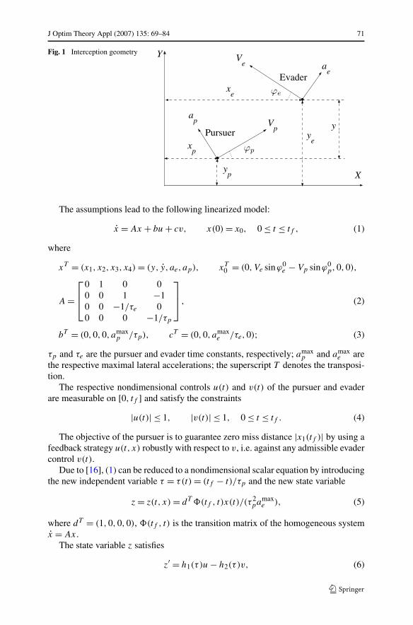
In Fig. 1 a schematic view of the interception geometry is shown. The X axis of thecoordinate system is aligned with the initial line of sight. The origin is collocated withthe initial pursuer position. The points (xp, yp), (xe, ye) are the current coordinatesof the objects; Vp and Ve are the velocities of the pursuer and evader; ap , ae are thelateral accelerations of the pursuer and evader, respectively; ϕp,ϕe are the respectiveangles between the velocity vectors and the reference line of sight; and y = ye − yp

is the relative separation normal to the initial line of sight.It is assumed that the angles ϕp , ϕe are sufficiently small, yielding the approx-

imation cosϕi ≈ 1, sinϕi ≈ ϕi , i = p, e. As a consequence, the trajectories of thepursuer and the evader can be linearized with respect to the nominal collision geom-etry, leading to a constant closing velocity Vc . The final interception time tf can beeasily calculated for any given initial conditions: tf = r0/Vc, where r0 is the initialdistance between the objects and the initial time t0 = 0.

J Optim Theory Appl (2007) 135: 69–84 71

Fig. 1 Interception geometry

The assumptions lead to the following linearized model:

x = Ax + bu + cv, x(0) = x0, 0 ≤ t ≤ tf , (1)

where

xT = (x1, x2, x3, x4) = (y, y, ae, ap), xT0 = (0,Ve sinϕ0

e − Vp sinϕ0p,0,0),

A =⎡⎢⎣

0 1 0 00 0 1 −10 0 −1/τe 00 0 0 −1/τp

⎤⎥⎦ , (2)

bT = (0,0,0, amaxp /τp), cT = (0,0, amax

e /τe,0); (3)

τp and τe are the pursuer and evader time constants, respectively; amaxp and amax

e arethe respective maximal lateral accelerations; the superscript T denotes the transposi-tion.

The respective nondimensional controls u(t) and v(t) of the pursuer and evaderare measurable on [0, tf ] and satisfy the constraints

|u(t)| ≤ 1, |v(t)| ≤ 1, 0 ≤ t ≤ tf . (4)

The objective of the pursuer is to guarantee zero miss distance |x1(tf )| by using afeedback strategy u(t, x) robustly with respect to v, i.e. against any admissible evadercontrol v(t).

Due to [16], (1) can be reduced to a nondimensional scalar equation by introducingthe new independent variable τ = τ(t) = (tf − t)/τp and the new state variable

z = z(t, x) = dT �(tf , t)x(t)/(τ 2pamax

e ), (5)

where dT = (1,0,0,0), �(tf , t) is the transition matrix of the homogeneous systemx = Ax.

The state variable z satisfies

z′ = h1(τ )u − h2(τ )v, (6)


where a prime denotes derivative with respect to τ , with

h1(τ ) � μ(exp(−τ) + τ − 1) = μh(τ), (7)

h2(τ ) � ε(exp(−τ/ε) + τ/ε − 1) = εh(τ/ε), (8)

h(ξ) = exp(−ξ) + ξ − 1, (9)

μ = amaxp /amax

e , ε = τe/τp. (10)

The initial condition is

z(τ0) = z0 = ((Ve sinϕ0e − Vp sinϕ0

p)τ0)/(τpamaxe ), (11)

where τ0 = tf /τp .Due to (5), the controls u(t) and v(t) become u(tf − τpτ) and v(tf − τpτ), re-

spectively, denoted in the sequel as u(τ) and v(τ). The constraints (4) in the nondi-mensional formulation become

|u(τ)| ≤ 1, |v(τ)| ≤ 1, 0 ≤ τ ≤ τ0. (12)

Since z(0) = x1(tf )/(τ 2pamax

e ) (see (5)), the original pursuer objective can be refor-mulated for the scalar system (6): to guarantee z(0) = 0 by using a feedback strategyu(τ, z) robustly with respect to v(τ). If a strategy u∗(τ, z) solves the scalar intercep-tion problem, then the strategy u(t, x) = u∗(τ (t), z(t, x)) solves the original problemfor (1).

3 Previous Results

3.1 Capture Zones of Linear Feedback Strategies

In this subsection, the general results of [15] on capture zones of linear strategies arebriefly summarized.

Let u(τ, z) = K(τ)z be a linear pursuer strategy, with the time varying gain K(τ)

such that:

(K1) K(τ) > 0 for τ > 0.(K2) K(τ) is continuously differentiable for τ > 0.(K3) For some α = α(K(·)) > 0, there exist finite limits

limτ→0

K(τ)τα = C = C(α) > 0, (13)

limτ→0

K ′(τ )τα+1 = −αC. (14)

Note that, for any K(·) satisfying (K1)–(K3), any initial condition and any admis-sible evader control v(τ), there exist a unique solution zK(τ) = zK(τ, τ0, z0, v(·)) of(6) on (0, τ0] and a finite limit limτ→0 zK(τ) � zK(0).

The set C = C(K(·)) of initial positions (τ0, z0) is called the (robust) capture zoneof a linear strategy u(·) if, for (τ0, z0) ∈ C and for any admissible evader control v(τ),the conditions below are satisfied:


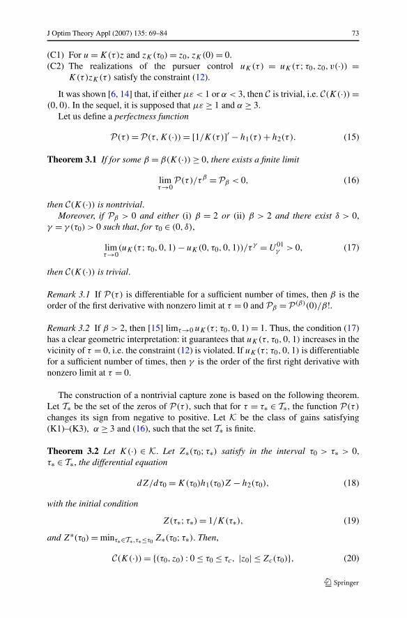
(C1) For u = K(τ)z and zK(τ0) = z0, zK(0) = 0.(C2) The realizations of the pursuer control uK(τ) = uK(τ ; τ0, z0, v(·)) =

K(τ)zK(τ) satisfy the constraint (12).

It was shown [6, 14] that, if either με < 1 or α < 3, then C is trivial, i.e. C(K(·)) =(0,0). In the sequel, it is supposed that με ≥ 1 and α ≥ 3.

Let us define a perfectness function

P(τ ) = P(τ,K(·)) = [1/K(τ)]′ − h1(τ ) + h2(τ ). (15)

Theorem 3.1 If for some β = β(K(·)) ≥ 0, there exists a finite limit

limτ→0

P(τ )/τβ = Pβ < 0, (16)

then C(K(·)) is nontrivial.Moreover, if Pβ > 0 and either (i) β = 2 or (ii) β > 2 and there exist δ > 0,

γ = γ (τ0) > 0 such that, for τ0 ∈ (0, δ),

limτ→0

(uK(τ ; τ0,0,1) − uK(0, τ0,0,1))/τγ = U01γ > 0, (17)

then C(K(·)) is trivial.

Remark 3.1 If P(τ ) is differentiable for a sufficient number of times, then β is theorder of the first derivative with nonzero limit at τ = 0 and Pβ = P(β)(0)/β!.

Remark 3.2 If β > 2, then [15] limτ→0 uK(τ ; τ0,0,1) = 1. Thus, the condition (17)has a clear geometric interpretation: it guarantees that uK(τ, τ0,0,1) increases in thevicinity of τ = 0, i.e. the constraint (12) is violated. If uK(τ ; τ0,0,1) is differentiablefor a sufficient number of times, then γ is the order of the first right derivative withnonzero limit at τ = 0.

The construction of a nontrivial capture zone is based on the following theorem.Let T∗ be the set of the zeros of P(τ ), such that for τ = τ∗ ∈ T∗, the function P(τ )

changes its sign from negative to positive. Let K be the class of gains satisfying(K1)–(K3), α ≥ 3 and (16), such that the set T∗ is finite.

Theorem 3.2 Let K(·) ∈ K. Let Z∗(τ0; τ∗) satisfy in the interval τ0 > τ∗ > 0,τ∗ ∈ T∗, the differential equation

dZ/dτ0 = K(τ0)h1(τ0)Z − h2(τ0), (18)

with the initial condition

Z(τ∗; τ∗) = 1/K(τ∗), (19)

and Z∗(τ0) = minτ∗∈T∗,τ∗≤τ0 Z∗(τ0; τ∗). Then,

C(K(·)) = {(τ0, z0) : 0 ≤ τ0 ≤ τc, |z0| ≤ Zc(τ0)}, (20)


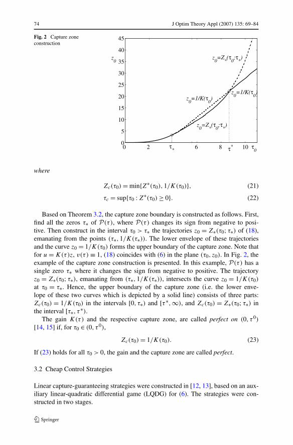
Fig. 2 Capture zoneconstruction

where

Zc(τ0) = min{Z∗(τ0),1/K(τ0)}, (21)

τc = sup{τ0 : Z∗(τ0) ≥ 0}. (22)

Based on Theorem 3.2, the capture zone boundary is constructed as follows. First,find all the zeros τ∗ of P(τ ), where P(τ ) changes its sign from negative to posi-tive. Then construct in the interval τ0 > τ∗ the trajectories z0 = Z∗(τ0; τ∗) of (18),emanating from the points (τ∗,1/K(τ∗)). The lower envelope of these trajectoriesand the curve z0 = 1/K(τ0) forms the upper boundary of the capture zone. Note thatfor u = K(τ)z, v(τ) ≡ 1, (18) coincides with (6) in the plane (τ0, z0). In Fig. 2, theexample of the capture zone construction is presented. In this example, P(τ ) has asingle zero τ∗ where it changes the sign from negative to positive. The trajectoryz0 = Z∗(τ0; τ∗), emanating from (τ∗,1/K(τ∗)), intersects the curve z0 = 1/K(τ0)

at τ0 = τ∗. Hence, the upper boundary of the capture zone (i.e. the lower enve-lope of these two curves which is depicted by a solid line) consists of three parts:Zc(τ0) = 1/K(τ0) in the intervals [0, τ∗) and [τ ∗,∞), and Zc(τ0) = Z∗(τ0; τ∗) inthe interval [τ∗, τ ∗).

The gain K(τ) and the respective capture zone, are called perfect on (0, τ 0)

[14, 15] if, for τ0 ∈ (0, τ 0),

Zc(τ0) = 1/K(τ0). (23)

If (23) holds for all τ0 > 0, the gain and the capture zone are called perfect.

3.2 Cheap Control Strategies

Linear capture-guaranteeing strategies were constructed in [12, 13], based on an aux-iliary linear-quadratic differential game (LQDG) for (6). The strategies were con-structed in two stages.


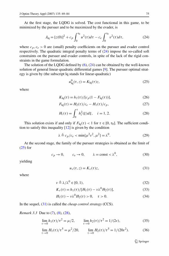
At the first stage, the LQDG is solved. The cost functional in this game, to beminimized by the pursuer and to be maximized by the evader, is

Jlq = [z(0)]2 + cp

∫ τ0

0u2(τ )dτ − ce

∫ τ0

0v2(τ )dτ, (24)

where cp, ce > 0 are (small) penalty coefficients on the pursuer and evader controlrespectively. The quadratic integral penalty terms of (24) impose the so-called softconstraints on the pursuer and evader controls, in spite of the lack of the rigid con-straints in the game formulation.

The solution of the LQDG defined by (6), (24) can be obtained by the well-knownsolution of general linear-quadratic differential games [9]. The pursuer optimal strat-egy is given by (the subscript lq stands for linear-quadratic)

u0lq(τ, z) = Klq(τ )z, (25)

where

Klq(τ ) = h1(τ )/[cp(1 − Flq(τ ))], (26)

Flq(τ ) = H2(τ )/ce − H1(τ )/cp, (27)

Hi(τ) =∫ τ

0h2

i (ξ)dξ, i = 1,2. (28)

This solution exists if and only if Flq(τ ) < 1 for τ ∈ [0, τ0]. The sufficient condi-tion to satisfy this inequality [12] is given by the condition

λ � cp/ce < min{μ2ε2,μ2} = λ0. (29)

At the second stage, the family of the pursuer strategies is obtained as the limit of(25) for

cp → 0, ce → 0, λ = const < λ0, (30)

yielding

uν(τ, z) = Kν(τ)z, (31)

where

ν � λ/λ0 ∈ [0,1), (32)

Kν(τ) = h1(τ )/[H1(τ ) − νλ0H2(τ )], (33)

H1(τ ) − νλ0H2(τ ) > 0, τ > 0. (34)

In the sequel, (31) is called the cheap control strategy (CCS).

Remark 3.3 Due to (7), (8), (28),

limτ→0

h1(τ )/τ 2 = μ/2, limτ→0

h2(τ )/τ 2 = 1/(2ε), (35)

limτ→0

H1(τ )/τ 5 = μ2/20, limτ→0

H2(τ )/τ 5 = 1/(20ε2). (36)


Therefore, by virtue of (29) and (33), α(Kν(·)) = 3 and in (13),

C = 10ε2/[μ(ε2 − νψ(ε))], (37)

where

ψ(ε) = min(ε2,1). (38)

Note that

ε2 − νψ(ε) > 0, for any ε > 0, ν ∈ [0,1).

In this paper, the general Theorems 3.1, 3.2 are applied to the CCS providing a de-tailed analytical and numerical description of the CCS capture zone for all admissiblevalues of the parameters μ, ε and ν.

4 Existence of Nontrivial Capture Zone

The following lemmas, proven in the Appendix, provide the values of β , Pβ and U01γ

for the CCS.

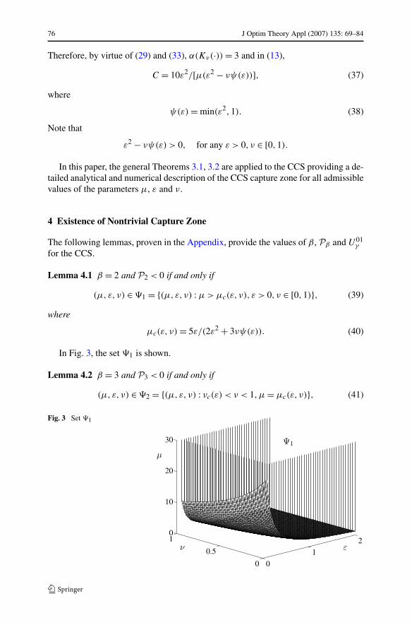
Lemma 4.1 β = 2 and P2 < 0 if and only if

(μ, ε, ν) ∈ �1 = {(μ, ε, ν) : μ > μc(ε, ν), ε > 0, ν ∈ [0,1)}, (39)

where

μc(ε, ν) = 5ε/(2ε2 + 3νψ(ε)). (40)

In Fig. 3, the set �1 is shown.


(μ, ε, ν) ∈ �2 = {(μ, ε, ν) : νc(ε) < ν < 1,μ = μc(ε, ν)}, (41)

Fig. 3 Set �1


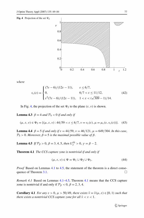
Fig. 4 Projection of the set �2

where

νc(ε) =

⎧⎪⎨⎪⎩

(7ε − 6)/(12ε − 11), ε ≤ 6/7,

0, 6/7 < ε ≤ 11/12,

ε2(7ε − 6)/(12ε − 11), 1 < ε < (√

309 − 1)/14.

(42)

In Fig. 4, the projection of the set �2 to the plane (ε, ν) is shown.


(μ, ε, ν) ∈ �3 = {(μ, ε, ν) : 44/59 < ε ≤ 6/7, ν = νc(ε),μ = μc(ε, νc(ε))}. (43)

Lemma 4.4 β = 5 if and only if ε = 44/59, ν = 46/121, μ = 649/304. In this case,P5 > 0. Moreover, β = 5 is the maximal possible value of β .

Lemma 4.5 If Pβ > 0, β = 3,4,5, then U01γ > 0, γ = β − 2.

Theorem 4.1 The CCS capture zone is nontrivial if and only if

(μ, ε, ν) ∈ � = �1 ∪ �2 ∪ �3. (44)

Proof Based on Lemmas 4.1 to 4.5, the statement of the theorem is a direct conse-quence of Theorem 3.1. �

Remark 4.1 Based on Lemmas 4.1–4.5, Theorem 4.1 means that the CCS capturezone is nontrivial if and only if Pβ < 0, β = 2,3,4.

Corollary 4.1 For any ε > 0, μ > 50/49, there exists ν = ν(μ, ε) ∈ [0,1) such thatthere exists a nontrivial CCS capture zone for all ν < ν < 1.


Proof The inequality μ > μc(ε, ν), guaranteeing the existence of a nontrivial CCScapture zone, is valid if

(5ε − 2ε2μ)/(3μψ(ε)) < ν < 1, (45)

where

μ > 5ε/(2ε2 + 3ψ(ε)). (46)

For ε ≤ 1, the inequality (46) is equivalent to με > 1, which is valid by assump-tion. Note that

maxε>1

5ε/(2ε2 + 3ψ(ε)) = maxε>1

5ε/(2ε2 + 3) = 50/49. (47)

This, together with (45), (46), completes the proof of the corollary. �

5 Capture Zone Construction

Theorem 5.1 For any ε > 0, ν ∈ [0,1), there exists μ0 = μ0(ε, ν) > 0 such that if

μ ≥ μ0, (48)

and (μ, ε, ν) ∈ � , then the CCS capture zone is perfect.

Proof Due to Theorem 3.2 and Remark 4.1, it is sufficient to prove the existence ofμ0(ε, ν) > 0 such that (48) yields P(τ ) ≤ 0 for all τ > 0. It can be directly shownthat the inequality P(τ ) ≤ 0 is equivalent to

h2(τ )h2(τ ) − μ(νψ(ε)(h(τ)h22(τ ) − h′(τ )H2(τ )) + h′(τ )H(τ)) ≤ 0, (49)

where h2(τ ), h(τ) and H2(τ ) are defined by (8), (9) and (28), respectively; H(τ) =H1(τ ) for μ = 1. The function

W(τ) � h2(τ )h2(τ )/[νψ(ε)[h(τ)h22(τ ) − h′(τ )H2(τ )] + h′(τ )H(τ)], (50)

is continuous for τ > 0 and, by direct calculation,

limτ→0

W(τ) = 5ε/(2ε2 + 3νψ(ε)), (51)

limτ→∞W(τ) = 3/(1 + 2νψ(ε)). (52)

Hence, by virtue of (49),

μ0(ε, ν) = supτ≥0

W(τ), (53)

which completes the proof. �


Fig. 5 Graphs of μ0(ε, ν)

Fig. 6 Graphs of ν0(μ, ε)

Remark 5.1 The function 1/Kν(τ) increases monotonically for τ > 0. Hence, forμ ≥ μ0, the CCS capture zone is unbounded with respect to τ0 and z0.

In Fig. 5, the values of μ0 are presented as functions of ε for different values of ν.It is seen that the larger is the value of ν, the smaller is the value of μ, ensuring theperfectness (and consequently the unboundedness) of the CCS capture zone.

Corollary 5.1 For any ε > 0, μ > μ0(ε,0), there exists ν0 = ν0(μ, ε) ∈ [0,1) suchthat the CCS capture zone is perfect for all ν0 ≤ ν < 1.

The corollary is proven similarly to Corollary 4.1. In Fig. 6, ν0 is shown as afunction of ε for three values of μ.

The examples of perfect capture zones are shown in Fig. 7 for ε = 1.2 and ν = 0,0.5, 0.9. In this case μ = 3 ≥ μ0(1.2, ν) for all chosen values of ν. It is seen that,for the same values of μ and ε, the smaller is the value of ν, the larger is the capturezone.


Fig. 7 Perfect capture zones

Observation 5.1 Extensive numerical study shows that, if (μ, ε, ν) ∈ � , then forμ < μ0(ε, ν) the function P(τ ) = P(τ,Kν(·)) has only a single zero τ∗ where P(τ )

changes its sign from negative to positive.

Proposition 5.1 If

μ < μ1(ε, ν) � 3/(1 + 2νψ(ε)), (54)

and (μ, ε, ν) ∈ � , then

Zc(τ0) ={

1/Kν(τ0), 0 ≤ τ0 < τ∗,Z∗(τ0; τ∗), τ∗ ≤ τ0 ≤ τc,

(55)

where Z∗(τ0; τ∗) satisfies (18) for K(τ0) = Kν(τ0), τc = sup{τ0 :Z∗(τ0; τ∗) ≥ 0}.

Proof The inequality (54) is equivalent to limτ→∞ P(τ ) > 0. Due to Remark 4.1 andObservation 5.1, this means that in this case, P(τ ) has a single root. Hence, due toTheorem 3.2, the capture zone boundary is given by (55). �

Remark 5.2 Numerical simulation shows that limτ0→∞ Z∗(τ0; τ∗) = −∞, yielding afinite value of τc. This means that in this case, the CCS capture zone is bounded.

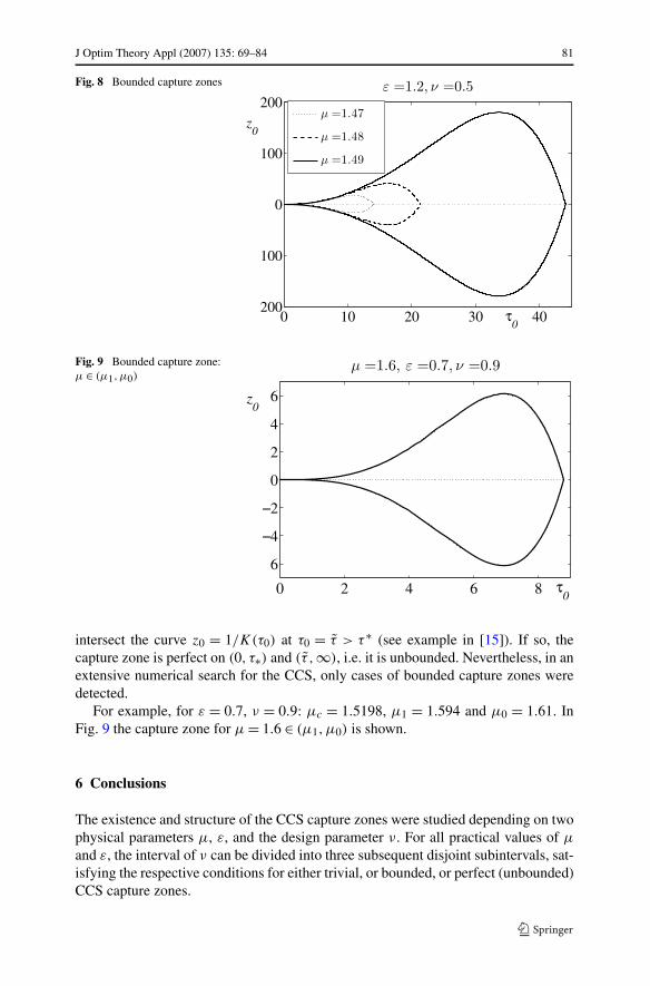
The examples of bounded capture zones are shown in Fig. 8 for ε = 1.2, ν = 0.5and μ = 1.47, 1.48, 1.49 ∈ (μc,μ1) = (1.37,1.5). It is seen that the larger is thevalue of μ, the larger is the capture zone.

Remark 5.3 Due to (52–54), for any admissible ε, ν: μ1(ε, ν) ≤ μ0(ε, ν).

If μ1 < μ0 and μ ∈ (μ1,μ0), then P(τ ) has two zeros: τ∗ ∈ T∗ and τ ∗ > τ∗.In principle (for some other gains K(τ)), in this case, the trajectory Z∗(τ0; τ∗) can


Fig. 8 Bounded capture zones

Fig. 9 Bounded capture zone:μ ∈ (μ1,μ0)

intersect the curve z0 = 1/K(τ0) at τ0 = τ > τ ∗ (see example in [15]). If so, thecapture zone is perfect on (0, τ∗) and (τ ,∞), i.e. it is unbounded. Nevertheless, in anextensive numerical search for the CCS, only cases of bounded capture zones weredetected.

For example, for ε = 0.7, ν = 0.9: μc = 1.5198, μ1 = 1.594 and μ0 = 1.61. InFig. 9 the capture zone for μ = 1.6 ∈ (μ1,μ0) is shown.

6 Conclusions

The existence and structure of the CCS capture zones were studied depending on twophysical parameters μ, ε, and the design parameter ν. For all practical values of μ

and ε, the interval of ν can be divided into three subsequent disjoint subintervals, sat-isfying the respective conditions for either trivial, or bounded, or perfect (unbounded)CCS capture zones.


Appendix Proofs of Lemmas

Proof of Lemma 4.1 By direct calculation, P(0) = P ′(0) = 0. Due to (15), (35)and (37),

limτ→0

P(τ )/τ 2 = (5ε − μ(2ε2 + 3ψ(ε)))/(10ε2). (56)

Hence, β = 2 and P2 < 0 if and only if μ > μc, where μc is given by (40). Thiscompletes the proof of Lemma 4.1. �

Proof of Lemma 4.2 Due to (56), P ′′(0) = 0 if and only if μ = μc(ε, ν). In this case,by direct calculation,

P ′′′(0) ={

(7ε − 6 − ν(12ε − 11))/(3ε2(3ν + 2)), ε ≤ 1,

(ε2(7ε − 6) − ν(12ε − 11))/(3ε2(3ν + 2ε2)), ε > 1.(57)

Hence, in this case, the inequality P ′′′(0) < 0, yielding β = 3 and P3 < 0, is equiva-lent to

0 ≤ ν < 1, ν > νc(ε), (58)

where

νc(ε) ={

(7ε − 6)/(12ε − 11), ε ≤ 1,

ε2(7ε − 6)/(12ε − 11), ε > 1.(59)

Note that νc ≤ 0 for 6/7 ≤ ε < 11/12; νc ≥ 1 for 11/12 < ε ≤ 1 and ε ≥(√

309 − 1)/14. Hence, for μ = μc , (58) is equivalent to νc(ε) < ν < 1, where νc

is given by (42). This inequality yields the inclusion (41), completing the proof ofLemma 4.2. �

Proof of Lemma 4.3 Due to (42), (56) and (57), P ′′(0) = P ′′′(0) = 0 if and only if0 ≤ ε ≤ 6/7 or 1 < ε < (

√309 − 1)/14, ν = νc(ε) and μ = μc(ε, νc(ε)). In this case,

by direct calculation,

P(IV)(0) ={

(ε − 1)2(59ε − 44)/7(9ε − 8), ε ≤ 6/7,

(ε − 1)2(59ε − 44)/7ε3(9ε − 8), 1 < ε < (√

309 − 1)/14,(60)

and P(IV)(0) < 0 if and only if 44/59 < ε ≤ 6/7. This implies that β = 4 and P4 < 0,completing the proof of Lemma 4.3. �

Proof of Lemma 4.4 Due to (56), (57) and (60), P ′′(0) = P ′′′(0) = P(IV)(0) = 0if and only if ε = εc = 44/59, ν = νc(εc) = 46/121, and μ = μc(εc, νc(εc)) =649/304. By direct calculation, in this case, P(V)(0) ≈ 0.0673, i.e. β = 5 and P5 > 0.This completes the proof of Lemma 4.4. �

Proof of Lemma 4.5 Let μ = μc(ε, ν), i.e. β = 3. Now, calculate the limit

U011 (τ0) = lim

τ→0u′

K(τ, τ0,0,1) = limτ→0

(K(τ)zK(τ, τ0,0,1))′. (61)


Due to (6),

u′K(τ, τ0,0,1) = K ′(τ )zK(τ, τ0,0,1) + K(τ)z′

K(τ, τ0,0,1)

= (K ′(τ ) + K2(τ )h1(τ ))zK(τ, τ0,0,1) − K(τ)h2(τ )

= Q(τ)uK(τ, τ0,0,1) − K(τ)h2(τ ), (62)

where

Q(τ) = K ′(τ )/K(τ) + K(τ)h1(τ ). (63)

Since β > 2, due to [15], limτ→0 uK(τ, τ0,0,1) = 1; consequently, in the vicinityof τ = 0, the function uK(τ, τ0,0,1) is given by

uK(τ, τ0,0,1) = 1 + τu′K(τ , τ0,0,1), τ ∈ (0, τ ). (64)

For τ → 0, this yields

U011 (τ0) = lim

τ→0(Q(τ) − K(τ)h2(τ ))/(1 − Q(τ)τ)

= limτ→0

K(τ)(K ′(τ )/K2(τ ) + h1(τ ) − h2(τ ))/(1 − Q(τ)τ)

= limτ→0

K(τ)P(τ )/(Q(τ)τ − 1). (65)

By virtue of (65) and direct calculation,

U011 (τ0) = ε(3ν + 2ψ(ε))P3/3(4ν + ψ(ε)). (66)

Note that U011 is independent of τ0 and has the same sign as P3.

By using a similar technique, for ν = νc(ε), μ = μc(ε, νc(ε), it can be derived that

U012 (τ0) = lim

τ→0(K(τ)P(τ ))′/(Q′(τ )τ 2/2 + Q(τ)τ − 1)

= ε(9ε − 8)P4/6(7ε − 6). (67)

Recall that P4 < 0 if and only if 44/59 < ε ≤ 6/7 and that P4 > 0 if and only if1 < ε < (

√309 − 1)/14. In both cases, (9ε − 9)/(7ε − 6) > 0, i.e., due to (67), U01

2has the same sign as P4.

Similarly, it can be shown that, for ε = 44/59, ν = 46/121, and μ = 649/304,U01

3 > 0. This completes the proof of Lemma 4.5. �

References

1. Letov, A.M.: Analytical controller design I–III. Autom. Remote Control 21, 303–306 (1960); 21,389–393 (1960); 21, 458–461 (1960); translation from Avtomatika i Telemekhanika 21, 436–441;561–568; 661–665 (1960)

2. Kalman, R.E.: Contributions to the theory of optimal control. Bol. Soc. Mat. Mex. 5, 102–119 (1960)3. Zarchan, P.: Tactical and Strategic Missile Guidance, 2nd edn. Progress in Astronautics and Aeronau-

tics, vol. 157. AIAA, Reston (1994)


4. Cottrell, R.G.: Optimal intercept guidance for short-range tactical missiles. AIAA J. 9, 1414–1415(1971)

5. Gutman, S., Leitmann, G.: Optimal strategies in the neighborhood of a collision course. AIAA J. 14,1210–1212 (1976)

6. Gutman, S.: On optimal guidance for homing missiles. J. Guid. Control Dyn. 3, 296–300 (1979)7. Shinar, J.: Solution techniques for realistic pursuit-evasion games. In: Leondes, C.T. (ed.) Advances

in Control and Dynamic Systems, vol. 17, pp. 63–124. Academic, New York (1981)8. Shima, T., Shinar, J.: Time-varying linear pursuit-evasion game models with bounded controls.

J. Guid. Control Dyn. 25, 425–432 (2002)9. Bryson, A.E., Ho, Y.C.: Applied Optimal Control. Hemisphere, New York (1975)

10. Ben-Asher, J., Yaesh, I.: Advances in Missile Guidance Theory. Progress in Astronautics and Aero-nautics, vol. 180. AIAA, Reston (1998)

11. Petersen, I.R.: Linear-quadratic differential games with cheap control. Syst. Control Lett. 8, 181–188(1986)

12. Turetsky, V., Shinar, J.: Missile guidance laws based on pursuit-evasion game formulations. Automat-ica 39, 607–618 (2003)

13. Turetsky, V.: Upper bounds of the pursuer control based on a linear-quadratic differential game. J. Op-tim. Theory Appl. 121, 163–191 (2004)

14. Turetsky, V., Glizer, V.Y.: Capture-guaranteeing pursuer linear strategies. 45th Israel Annual Confer-ence on Aerospace Sciences, Haifa, Tel Aviv, Israel (2005)

15. Turetsky, V.: Capture zone geometry of linear pursuit strategies. Report TAE 959. Technion, IsraelInstitute of Technology (2005)

16. Krasovskii, N.N., Subbotin, A.I.: Game-Theoretical Control Problems. Springer, New York (1988)

capture zones of cheap control interception strategies

Documents