capm-based optimal portfolios - stata€¦ · * i save the complete matrix in cell b1. capture...

CAPM-based optimal portfolios

Carlos Alberto Dorantes, Tec de Monterrey

2019 Chicago Stata Conference

Carlos Alberto Dorantes, Tec de Monterrey CAPM-based optimal portfolios 2019 Chicago Stata Conference 1 / 1

Outline

Data collection of financial data

The CAPM model and Portfolio Theory

Automating stock selection and portfolio optimization

Results of the automation process

Conclusions


Data collection of financial datagetsymbols easily downloads and process data from Quandl, Yahoo Finance,and Alpha Vantage. Here an example of daily prices of two stocks:

. * ssc install getsymbols

. cap getsymbols SBUX CAG, fy(2017) yahoo clear

. tsline adjclose_SBUX adjclose_CAG

Figure 1: Starbucks and Canagra prices


. . . Data collection of financial dataGetting monthly prices and calculating returns from several instrumentsfrom Yahoo:

. cap getsymbols ^GSPC SBUX CAG, fy(2014) freq(m) yahoo clear price(adjclose)

. *With the price option, returns are calculated

. cap gen year=yofd(dofm(period))

. graph box R_*, by(year, rows(1))

Figure 2: Box plot of monthly returns by year


The CAPM model and Portfolio Theory

Overview of Portfolio Theory

The CAPM model

Relationship between CAPM and Portfolio Theory


Overview of Portfolio Theory

The paper “Portfolio Selection” written in 1952 by Harry Markowitz was thebeginning of Modern Portfolio Theory (MPT)

Nobody before Markowitz had provided a rigorous framework to constructand select assets in a portfolio based on expected asset returns and thesystematic and unsystematic risk of a portfolio.

With the mean-variance analysis, Markowitz proposes a way to measureportfolio risk based on the variance-covariance matrix of asset returns

He discovered that the relationship between risk and return is not alwayslinear; he proposes a way to estimate the efficient frontier, and found that itis quadratic. It is possible to build portfolios that maximize expected returnand also minimize risk


The CAPM model

Under the theoretical framework of MPT, in the late 1950’s and early1960’s, the Capital Asset Pricing Theory was developed. The maincontributors were James Tobin, John Litner and William Sharpe.

They showed that the efficient frontier is transformed from quadratic to alinear function (the Capital Market Line) when a risk-free rate is added to aportfolio of stocks

The Tangency (optimal) Portfolio is the portfolio that touches both, theCML and the efficient frontier


. . . The CAPM model

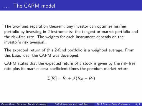
The two-fund separation theorem: any investor can optimize his/herportfolio by investing in 2 instruments: the tangent or market portfolio andthe risk-free rate. The weights for each instrument depends on theinvestor’s risk aversion.

The expected return of this 2-fund portfolio is a weighted average. Fromthis basic idea, the CAPM was developed.

CAPM states that the expected return of a stock is given by the risk-freerate plus its market beta coefficient times the premium market return:

E [Ri ] = Rf + β (RM − Rf )


Relationship between CAPM and Portfolio Theory

CAPM model can be used to1) estimate the expected return of a stock given an expected return of the

market. This estimate can be used as the expected stock return, thatis part if the inputs for MPT.

2) estimate the cost of equity or discount factor in the context of financialvaluation

3) select stocks for a portfolio based on the Jensen’s Alpha and/or marketbeta coefficients


Automating stock selection and portfolio optimization

CAPM estimation model

Writing a Stata command for the CAPM

Excel interface to easily change the input parameters

Stock selection based on the CAPM

Portfolio optimization

Portfolio backtesting


CAPM estimation model

To estimate the CAPM, I can run a time-series linear regression model usingmonthly continuously compounded returns. For this model, the dependentvariable is the premium stock return (excess stock return over the risk-freerate) and the independent variable is the premium market return:(

ri(t) − rf (t))

= α+ β(rM(t) − rf (t)

)+ εt

Note that I allow the model to estimate the constant (alpha of Jensen). Intheory, for a market to be in equilibrium, this constant must be zero, sincethere should not be a stock that systematically outperforms the market; inother words, a stock return should be determined by its market systematicrisk (beta) and its unsystematic/idiosyncratic risk (regression error)


Writing a command for the CAPM model

. capture program drop capm

. program define capm, rclass1. syntax varlist(min=2 max=2 numeric) [if], RFrate(varname)2. local stockret: word 1 of `varlist´3. local mktret: word 2 of `varlist´4. cap drop prem`stock´5. qui gen prem`stock´=`stockret´-`rfrate´6. cap drop mktpremium7. qui gen mktpremium=`mktret´-`rfrate´8. cap reg prem`stock´ mktpremium `if´9. if _rc==0 & r(N)>30 {

10. matrix res= r(table)11. local b1=res[1,1]12. local b0=res[1,2]13. local SEb1=res[2,1]14. local SEb0=res[2,2]15. local N=e(N)16. dis "Market beta is " %3.2f `b1´ "; std. error of beta is " %8.6f `SEb1´17. dis "Alpha is " %8.6f `b0´ "; std. error of alpha is " %8.6f `SEb0´18. return scalar b1=`b1´19. return scalar b0=`b0´20. return scalar SEb1=`SEb1´21. return scalar SEb0=`SEb0´22. return scalar N=`N´23. }24. end


. . .Writing a command for CAPM

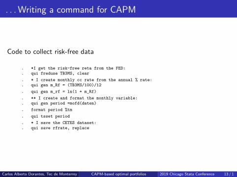
Code to collect risk-free data

. *I get the risk-free reta from the FED:

. qui freduse TB3MS, clear

. * I create monthly cc rate from the annual % rate:

. qui gen m_Rf = (TB3MS/100)/12

. qui gen m_rf = ln(1 + m_Rf)

. ** I create and format the monthly variable:

. qui gen period =mofd(daten)

. format period %tm

. qui tsset period

. * I save the CETES dataset:

. qui save rfrate, replace


. . . Writing a command for CAPM

Now I can use my capm command using monthly data of a stock:

. cap getsymbols ^GSPC CAG, fy(2014) freq(m) yahoo clear price(adjclose)

. * I merge the stock data with the risk-free dataset:

. qui merge 1:1 period using rfrate, keepusing(m_rf)

. qui drop if _merge!=3

. qui drop _merge

. qui save mydata1,replace

.

. capm r_CAG r__GSPC, rfrate(m_rf)Market beta is 0.87; std. error of beta is 0.259952Alpha is -0.003563; std. error of alpha is 0.008909. return listscalars:

r(N) = 65r(SEb0) = .0089092926405626r(SEb1) = .259951861344863

r(b0) = -.0035630903188013r(b1) = .8731915389793837


. . .Writing a command for CAPM

I can examine how market beta of a stock changes over time I run my capmcommand using 24-month rolling windows:

. rolling b1=r(b1) seb1=r(SEb1), window(24) saving(capmbetas,replace): ///> capm r_CAG r__GSPC, rfrate(m_rf)(running capm on estimation sample)Rolling replications (43)

1 2 3 4 5...........................................file capmbetas.dta saved.


. . .Writing a command for CAPMCode to show how beta moves over time

. qui use capmbetas,clear

. label var b1 "beta"

. qui tsset end

. tsline b1

Figure 3: Market beta over time for CANAGRA using 24-month windowsCarlos Alberto Dorantes, Tec de Monterrey CAPM-based optimal portfolios 2019 Chicago Stata Conference 16 / 1

CAPM-GARCH estimation model using daily data

. capture program drop capmgarch

. program define capmgarch, rclass1. syntax varlist(min=2 max=2 numeric) [if], RFrate(varname) timev(varname)2. local stockret: word 1 of `varlist´3. local mktret: word 2 of `varlist´4. tempvar stockpremium mktpremium5. tsset `timev´6. qui gen `stockpremium´=`stockret´-`rfrate´7. qui gen `mktpremium´=`mktret´-`rfrate´8. cap arch `stockpremium´ `mktpremium´ `if´, arch(1) garch(1) ar(1)9. if _rc==0 & r(N)>30 {

10. matrix res= r(table)11. local b1=res[1,1]12. local b0=res[1,2]13. local SEb1=res[2,1]14. local SEb0=res[2,2]15. local N=e(N)16. dis "Market beta is " %3.2f `b1´ "; std. error of beta is " %8.6f `SEb1´17. dis "Alpha is " %8.6f `b0´ "; std. error of alpha is " %8.6f `SEb0´18. return scalar b1=`b1´19. return scalar b0=`b0´20. return scalar SEb1=`SEb1´21. return scalar SEb0=`SEb0´22. return scalar N=`N´23. }24. end


Excel interface for automation of data collection

Figure 4: exceltemplate1, parameters Sheet



Figure 5: exceltemplate1, tickerssp Sheet



Figure 6: exceltemplate1, tickerssp Sheet



I will use all S&P500 tickers with valid monthly price data(dataset=2)

I will use monthly historical data from Jan 2015 to Dec 2017 to estimatethe CAPM models, select stocks and optimize the portfolio

I will use the period from Jan 2018 to Jun 2019 as the backtesting periodfor the CAPM-based investment strategy



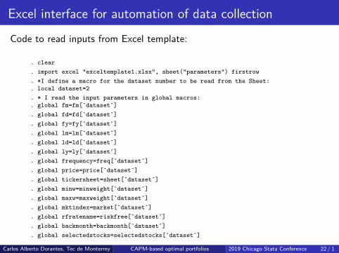
Code to read inputs from Excel template:

. clear

. import excel "exceltemplate1.xlsx", sheet("parameters") firstrow

. *I define a macro for the dataset number to be read from the Sheet:

. local dataset=2

. * I read the input parameters in global macros:

. global fm=fm[`dataset´]

. global fd=fd[`dataset´]

. global fy=fy[`dataset´]

. global lm=lm[`dataset´]

. global ld=ld[`dataset´]

. global ly=ly[`dataset´]

. global frequency=freq[`dataset´]

. global price=price[`dataset´]

. global tickersheet=sheet[`dataset´]

. global minw=minweight[`dataset´]

. global maxw=maxweight[`dataset´]

. global mktindex=market[`dataset´]

. global rfratename=riskfree[`dataset´]

. global backmonth=backmonth[`dataset´]

. global selectedstocks=selectedstocks[`dataset´]



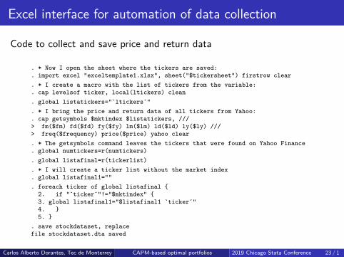
Code to collect and save price and return data

. * Now I open the sheet where the tickers are saved:

. import excel "exceltemplate1.xlsx", sheet("$tickersheet") firstrow clear

. * I create a macro with the list of tickers from the variable:

. cap levelsof ticker, local(ltickers) clean

. global listatickers="`ltickers´"

. * I bring the price and return data of all tickers from Yahoo:

. cap getsymbols $mktindex $listatickers, ///> fm($fm) fd($fd) fy($fy) lm($lm) ld($ld) ly($ly) ///> freq($frequency) price($price) yahoo clear. * The getsymbols command leaves the tickers that were found on Yahoo Finance. global numtickers=r(numtickers). global listafinal=r(tickerlist). * I will create a ticker list without the market index. global listafinal1="". foreach ticker of global listafinal {

2. if "`ticker´"!="$mktindex" {3. global listafinal1="$listafinal1 `ticker´"4. }5. }

. save stockdataset, replacefile stockdataset.dta saved



Code to collect and save the risk-free data

. clear

. *ssc install freduse

. freduse $rfratename(1,026 observations read). * I create monthly cc rate from the annual % rate:. gen m_Rf = ($rfratename/100)/12. * I calculate the continuously compounded return from the simple returns:. gen m_rf = ln(1 + m_Rf). * I create monthly variable for the months:. gen period =mofd(daten). format period %tm. * Now I indicate Stata that the time variable is period:. tsset period

time variable: period, 1934m1 to 2019m6delta: 1 month

. * I save the CETES dataset as cetes:

. save riskfdata, replacefile riskfdata.dta saved



Code to merge the stock dataset with the risk-free dataset

. *Now I open the stock data and do the merge:

. use stockdataset, clear(Source: Yahoo Finance!). merge 1:1 period using riskfdata, keepusing(m_rf)

Result # of obs.

not matched 973from master 1 (_merge==1)from using 972 (_merge==2)

matched 54 (_merge==3)

. * I keep only those raws that matched (_merge==3)

. keep if _merge==3(973 observations deleted). drop _merge. * I save the the dataset with the risk-free data:. save stockdataset, replacefile stockdataset.dta saved


Automating the estimation of all CAPM models

Code to create a matrix for the CAPM coefficients and std. errors

. * I rename the market return variable to avoid calculating

. * a CAPM for the market variable r__MXX:

. local varmkt=strtoname("$mktindex",0)

. local varmkt="r_`varmkt´"

. rename `varmkt´ rMKT

. * I define a matrix to store the beta coefficients and the p-values:

. * The macro $numtickers has the number of valid tickers found

. set matsize 600

. matrix BETAS=J($numtickers-1,5,0)

. matrix colnames BETAS= alpha beta se_alpha se_beta N



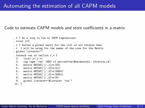
Code to estimate CAPM models and store coefficients in a matrix

. * I do a loop to run al CAPM regressions:

. local j=0

. * I define a global macro for the list of all returns that

. * I will be using for the names of the rows for the Matrix

. global listaret=""

. foreach var of varlist r_* {2. local j=`j´+13. cap capm `var´ rMKT if period<=tm($backmonth), rfrate(m_rf)4. matrix BETAS[`j´,1]=r(b0)5. matrix BETAS[`j´,2]=r(b1)6. matrix BETAS[`j´,3]=r(SEb0)7. matrix BETAS[`j´,4]=r(SEb1)8. matrix BETAS[`j´,5]=r(N)9. global listaret="$listaret `var´"

10. }



Code to show results stored in the matrix

. * I assign names to each row according to the ticker list:

. matrix rownames BETAS=$listaret

. matlist BETAS[1..8,.]alpha beta se_alpha se_beta N

r_A .0045485 1.541188 .0073556 .2520855 35r_AAL -.0060653 1.0219 .0152584 .5229235 35r_AAP -.0171335 .4446284 .0154508 .5295168 35

r_AAPL .0006362 1.384231 .0094234 .3229497 35r_ABBV .0058071 1.291651 .0095205 .3262765 35r_ABC -.0085388 1.063213 .0123592 .4235645 35r_ABT -.0050732 1.702326 .0073894 .2532439 35r_ACN .0105192 1.039847 .0064168 .2199101 35



Code to send results to excel

. * I set the Sheet where results will be sent :

. putexcel set exceltemplate1.xlsx, sheet("RESULTS`dataset´") modify

. * I save the complete matrix in cell B1

. capture putexcel B1=matrix(BETAS), names

. putexcel B1=matrix(BETAS,names)file exceltemplate1.xlsx saved. * I save the list of tickers in column A. putexcel A1=("ticker")file exceltemplate1.xlsx saved. local j=1. foreach ticker of global listafinal1 {

2. local j=`j´+13. quietly putexcel A`j´=("`ticker´")4. }


Stock selection based on CAPM coefficients

Code to create 95% C.I. of coefficients and select stocks

. * Importing the resulting sheet with the beta coefficients in to Stata:

. import excel using exceltemplate1, sheet("RESULTS`dataset´") firstrow clear

. * I generate the 95% confidence interval of alpha and beta:

. cap gen minalpha=alpha - abs(invttail(N,0.05)) * se_alpha

. cap gen maxalpha=alpha + abs(invttail(N,0.05)) * se_alpha

. cap gen minbeta=beta - abs(invttail(N,0.05)) * se_beta

. cap gen maxbeta=beta + abs(invttail(N,0.05)) * se_beta

. count if minalpha >=031

. display "Number of stocks with SIGNIFICANT AND POSITIVE ALPHA=" r(N)Number of stocks with SIGNIFICANT AND POSITIVE ALPHA=31.. keep if minalpha >=0 & minbeta>=0(451 observations deleted). * Now I will sort the stocks based on Alpha:. gsort -alpha. * I will keep the best stocks in terms of alpha:. capture keep in 1/$selectedstocks. * I save the best stock tickers in a Stata dataset. save besttickers`dataset´, replacefile besttickers2.dta saved


Portfolio optimization of the selected stocks

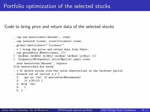
Code to bring price and return data of the selected stocks

. cap use besttickers`dataset´, clear

. cap levelsof ticker, local(ltickers) clean

. global besttickers="`ltickers´"

. * I bring the price and return data from Yahoo:

. cap getsymbols $besttickers, ///> fm($fm) fd($fd) fy($fy) lm($lm) ld($ld) ly($ly) ///> frequency($frequency) price($price) yahoo clear. save beststocks`dataset´, replacefile beststocks2.dta saved. * If delete stocks with few valid observations in the backtest period. foreach ret of varlist r_* {

2. qui su `ret´ if period>tm($backmonth)3. if r(N)<12 {4. drop `ret´5. }6. }


. . . Portfolio optimization of the selected stocksCode to optimize the portfolio with restrictions (before backmonth)

. ovport r_* if period<=tm($backmonth), minw($minw) max($maxw)Number of observations used to calculate expected returns and var-cov matrix :> 36The weight vector of the Tangent Portfolio with a risk-free rate of 0 (NOT Allo> w Short Sales) is:

Weightsr_ADBE .01884751r_ALGN .07281493r_AMZN .07410937r_CDNS .05888357r_NVDA .16591405r_PGR .3

r_TTWO .00943057r_UNH .3

The return of the Tangent Portfolio is: .03349151The standard deviation (risk) of the Tangent Portfolio is: .03429288

The marginal contributions to risk of the assets in the Tangent Portfolio are:Margina~k

r_ADBE .0272682r_ALGN .0464094r_AMZN .0334565r_CDNS .0258435r_NVDA .0701327r_PGR .0265421

r_TTWO .040259r_UNH .0214005

Type return list to see the portfolios in the Capital Market Line and the effic> ient frontierNumber of observations used to calculate expected returns and var-cov matrix :> 36The weight vector of the Tangent Portfolio with a risk-free rate of 0 (NOT Allo> w Short Sales) is:

Weightsr_ADBE .01884751r_ALGN .07281493r_AMZN .07410937r_CDNS .05888357r_NVDA .16591405r_PGR .3

r_TTWO .00943057r_UNH .3

The return of the Tangent Portfolio is: .03349151The standard deviation (risk) of the Tangent Portfolio is: .03429288The marginal contributions to risk of the assets in the Tangent Portfolio are:

Margina~k


r_TTWO .040259r_UNH .0214005


. . . Portfolio optimization of the selected stocksCode for the holding period return of the portfolio after backmonth

. matrix wop=r(weights)

. backtest p_* if period>tm($backmonth), weights(wop)It was assumed that the dataset is sorted chronologicallyThe holding return of the portfolio is .2614365819 observations/periods were used for the calculation (casewise deletion was ap> plied)The holding return of each price variable for the specified period was:

Price variable Return

p_adjclose_ADBE .5398479p_adjclose_ALGN .0785878p_adjclose_AMZN .3792017p_adjclose_CDNS .6763262p_adjclose_NVDA -.3201532p_adjclose_PGR .6445434

p_adjclose_TTWO -.0800505p_adjclose_UNH .1270745

The portfolio weights used were:

Asset Weight


r_TTWO .0094306r_UNH .3

. scalar retopt=r(retport)


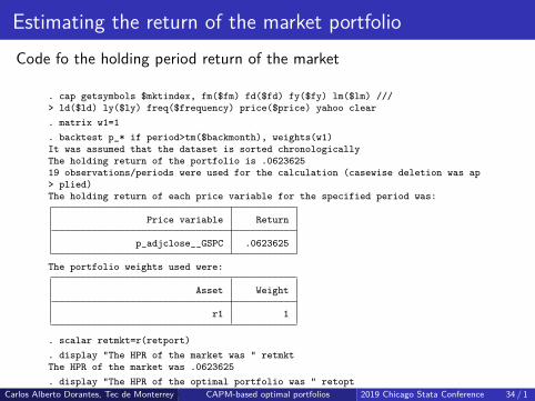
Estimating the return of the market portfolioCode fo the holding period return of the market

. cap getsymbols $mktindex, fm($fm) fd($fd) fy($fy) lm($lm) ///> ld($ld) ly($ly) freq($frequency) price($price) yahoo clear. matrix w1=1. backtest p_* if period>tm($backmonth), weights(w1)It was assumed that the dataset is sorted chronologicallyThe holding return of the portfolio is .062362519 observations/periods were used for the calculation (casewise deletion was ap> plied)The holding return of each price variable for the specified period was:

Price variable Return

p_adjclose__GSPC .0623625

The portfolio weights used were:

Asset Weight

r1 1

. scalar retmkt=r(retport)

. display "The HPR of the market was " retmktThe HPR of the market was .0623625. display "The HPR of the optimal portfolio was " retoptThe HPR of the optimal portfolio was .26143658Carlos Alberto Dorantes, Tec de Monterrey CAPM-based optimal portfolios 2019 Chicago Stata Conference 34 / 1

Exporting results to the Excel template

Code to export results to the Excel template

. putexcel set exceltemplate1.xlsx, sheet("parameters") modify

. putexcel Q1=("HPR Optimal Port") R1=("HPR Market")file exceltemplate1.xlsx saved. local row=`dataset´+1. putexcel Q`row´=(retopt)file exceltemplate1.xlsx saved. putexcel R`row´=(retmkt)file exceltemplate1.xlsx saved


Results of the automatic stock selection

Portfolio return of selected stocks was much higher than thebenchmark (market). For the holding period of 18 months, the optimalportfolio had a return around 26%, while the S&P 500 had a holdingreturn of around 6% (from Jan 2018 to Jun 2019)

Better results were obtained using bootstrapping for CAPM estimation(not shown here)

Better results were obtained using Exponential Weighted MovingAverage method for the estimation of expected stock return andexpected variance-covariance matrix (results not shown here)


Conclusions

Data collection and data management can be enhanced with interfacesbetween Stata and Excel

The getsymbols command along with commands from the mvportpackage are useful for financial data management and for constructingoptimal portfolios

Unlike other leading econometrics software, Stata has a simple scriptlanguage (do and ado files) that students can easily learn to betterunderstand Financial Econometrics


Thanks! Questions?

Carlos Alberto Dorantes, Ph.D.

Full-time professor

Accounting and Finance Department

Tecnológico de Monterrey, Querétaro Campus

[email protected]


capm-based optimal portfolios - stata€¦ · * i save the complete matrix in cell b1. capture...

Documents