Capital Supply and Corporate Bond Issuances:

Evidence From Mutual Fund Flows

Qifei Zhu∗

Abstract

This paper examines how idiosyncratic shocks to capital supply affect firms’

bond issuance decisions. Using bond funds’ holdings data, I establish an em-

pirical fact that funds that hold existing bonds of a company have a high

propensity to acquire new bonds from the same firm. Capital flows to a firm’s

existing bondholders hence affect firm-specific capital supply. Companies with

higher bondholder flows are more likely to issue bonds, enjoy lower yields, and

substitute away from equity financing and bank loans. I support the main re-

sults by using Bill Gross’ resignation from PIMCO as an exogenous shock to

the capital supply of affected companies.

∗Nanyang Business School, Nanyang Technological University. qifei.zhu@ntu.edu.sg. This paperis based on my PhD dissertation at the University of Texas at Austin. I am grateful to the membersof my dissertation committee, Andres Almazan, Jonathan Cohn, Clemens Sialm (co-Chair) andLaura Starks (co-Chair). I would also like to thank Aydogan Alti, Billy Grieser, Zack Liu, SheridanTitman, Vijay Yerramilli (discussant), Ben Zhang, and participants at the FIRS Conference andseminars at Baruch College, Nanyang Technological University, National University of Singapore,Singapore Management University, Southern Methodist University, University of New South Wales,University of Melbourne, University of Virginia, and University of Texas at Austin for their insightfulsuggestions and comments.

How does variation in the supply of different forms of capital affect firms’ financing

decisions? Traditionally, capital structure studies examine factors relating to firms’

demand for debt, such as taxes and distress costs. A burgeoning literature find

evidence that the capital structure of a company is significantly affected by the capital

availability of its creditors or investors (e.g. Faulkender and Petersen (2006), Leary

(2009), Sufi (2009)).1 These findings suggest a potentially important role for capital

supply in determining firms’ financing choices.

In this paper, I study how idiosyncratic shocks to investor capital affect firms’

decisions to issue bonds. Bond issuance is a major source of external financing for

U.S. companies.2 Unlike bank loans, bond issuance is thought to not depend on the

capital of specific investors: When a firm’s usual capital suppliers have insufficient

capital, firms should turn to a broad base of investors for financing. However, among

a sample of bond-investing mutual funds, I find significant “stickiness” in bond funds’

investment decisions: a firm’s current bondholders are much more likely to acquire

newly-issued bonds of the same company than investors who do not hold the previous

issues. This type of issuance-market segmentation implies that the capital supply of

a given firm may be affected by the capital availability of a small number of investors.

Building on this stylized fact, I construct a firm-specific variable, Bondholder Flow

(BHFlow), to capture shocks to a firm’s bond capital supply. BHFlow is defined as

the dollar amount of the capital supply from a firm’s existing bondholder funds scaled

by the firm’s outstanding bonds, under the assumption that bond funds proportion-

ally adjust their existing positions to flows. I find that bondholder flow positively

predicts the probability of firms’ future bond issuance, and negatively predicts bond

financing costs in the cross-section. Controlling for time fixed-effects, a one standard

1See also the survey evidence from Graham and Harvey (2001) and anecdotal evidence fromTitman (2002).

2During 1998–2014, U.S. non-financial companies issued USD 4.9 trillion of equity (gross ofrepurchases and M&A), USD 16.3 trillion of corporate bonds (gross), and obtained USD 5.8 trillionof commercial and industry loans (gross). See Figure 1 for the bond issuance volume in recent years.Source: Federal Reserve Bank; SIFMA

1

deviation increase in BHFlow predicts a 0.94 percentage point increase in the is-

suance probability next quarter (14 percent relative to the unconditional likelihood)

and a 5.5 basis points decline in offering yield spreads.

These results suggest a significant capital-supply effect on firms’ bond issuances.

It echos findings in Lemmon and Roberts (2010) and Chernenko and Sunderam (2012)

that corporate bond financing responds to market conditions. While the shocks used

in these previous papers affect the entire high yield segment relative to the investment

grade segment, the capital supply variations in my paper are firm-specific. To make

sure that the predictive power of BHFlow is not driven by systematic components in

fund flows, I further decompose fund-level flows into an expected component and the

residual, following the literature on mutual fund flows (e.g., Sirri and Tufano (1998);

Goldstein, Jiang, and Ng (2017)).3. Consistent with the baseline results, the residual

component predicts both issuance probability (positively) and offering yield spreads

(negatively).

I further rule out alternative explanations that demand-side factors drive the

observed relation between BHFlow and issuances. First, I find that a stronger bond-

holder flow predicts a lower probability of future equity issuances and bank loan

initiations. This alleviates the concern that bondholder flow covaries with firms’ to-

tal financing needs, or firms’ general demand for debt. Instead, firms seem to actively

trade off among various forms of capital (Baker (2009), Ma (2016)). Second, issuers

who raise bonds when bondholder flow is high spend a smaller fraction of issuance

proceeds in investments, as compared to other bond issuers. This contradicts what

one would expect if bondholder flow captures unobserved improvement in firms’ in-

vestment opportunities.

To further address the endogeneity concern, I utilize an unexpected shock to

bond fund flows derived from Bill Gross’ resignation from the Pacific Investment

3The explanatory variables for fund flow include past fund performances, fund size, fund age,investment objective of a fund, and the expense ratio of a funds.

2

Management Company (PIMCO). Bill Gross was the founder and CIO of PIMCO and

a well recognized fixed-income fund manager. His abrupt resignation from PIMCO

(presumably because of internal power struggle)4 in September of 2014 triggered

large redemption from all PIMCO mutual funds. I use this event as a negative

capital supply shock for companies who have a significant amount of bonds held

in PIMCO’s portfolios. In a difference-in-differences setting, I find that PIMCO’s

portfolio companies become significantly less likely to issue new bonds after Gross’

departure, relative to otherwise similar issuers.

The finding that corporate bond issuances are affected by individual bondholders’

capital is perhaps surprising when viewed through the lens of bank lending versus

arm’s-length financing. In bank lending, banks develop close relationships with their

borrowers through continuous monitoring (Boot (2000)). While bondholders in gen-

eral do not monitor their debtors, I hypothesize two economic mechanisms that may

create “stickiness” in their investment relationship. First, existing bondholders may

have lower information costs when they acquire new bonds: They have conducted

due diligence in the past and the information they gathered is “re-usable” (Chan,

Greenbaum, and Thakor (1986)). Second, existing bondholders may have repeated

relationships with the underwriters of bond issuances. Anecdotal evidence suggests

that some investment banks play favorites when allocating new bond issuances.5

Consistent with the information costs explanation, the propensity for existing

bondholders to participate in new bond offerings over regular investors is increasing in

firms’ degree of information asymmetry. For example, high-yield bond issuances rely

more heavily on the capital contribution of existing bondholders than investment-

grade ones do. I also find that high-information-asymmetry companies are more

responsive to bondholder flow in making bond issuance decisions. To test the under-

4For example, see “Bill Gross, King of Bonds, Abruptly Leaves Mutual Fund Giant PIMCO”,The New York Times, September 26, 2014

5“Regulators Are Probing How Goldman, Citi and Others Divvied Up Bonds”, Wall Street Jour-nal, Feb. 28, 2014

3

writer relationship explanation, I classify bond funds as “relationship investors” if a

fund has participated in prior bond offerings underwritten by the same investment

bank. I find that the status of being a relationship investor only explains a small

fraction of the effect of being an existing bondholder when mutual funds participate

in new bond offerings.

The findings in this paper contribute to several strands of literature. First, they

provide novel evidence for the supply effect on corporate capital structure. Traditional

capital structure studies tend to focus on the corporate demand for debt, while taking

capital supply as perfectly elastic, an assumption consistent with Modigliani and

Miller (1958). Several recent papers challenge this assumption, and they empirically

show that the supply of capital affects firms’ financing decisions (e.g. Faulkender

and Petersen (2006), Leary (2009), Sufi (2009), Lemmon and Roberts (2010)). A

common challenge for this nascent literature is to distinguish the supply effect from

the contamination of firms’ debt demand. To meet this identification challenge, Leary

(2009), Sufi (2009) and Lemmon and Roberts (2010) establish causality by utilizing

plausibly exogenous one-time shocks on the capital supply of specific market segments.

My paper uses a measure (BHFlow) that is firm-specific and applicable to all bond-

issuing firms. This allows comparisons within large cross-sections.

My paper also relates to the the literature on how equity issuance responds to

equity valuation.6 Khan, Kogan, and Serafeim (2012) show that the probability of

SEO increases when mutual fund shareholders receive large inflows. Gao and Lou

(2013) document that firms switch to debt financing when their equity prices are

temporarily depressed by mutual fund fire sales.7 Compared to equity issuances,

bond issuances are more frequent, and they constitute a larger amount of corporate

external financing. More importantly, the lack of liquidity in the secondary corporate

6For example, see Baker and Wurgler (2002); Baker, Stein, and Wurgler (2003); and Alti andSulaeman (2012) for equity SEOs, and Alti (2006) for IPOs.

7Also related is Edmans, Goldstein, and Jiang (2012)), who show that undervaluation inducedby mutual fund fire sales increases takeover probability.

4

bond market (Edwards, Harris, and Piwowar (2007); Bao, Pan, and Wang (2011))

amplifies the impact of bondholder flows. The low liquidity makes it costly for funds

to accommodate their flows via secondary-market trading. As a result, companies

are in a unique position to meet their investors’ increased flow-driven demand by

issuing new bonds. Empirically, I findt that firms whose outstanding bonds are less

frequently traded are particularly sensitive to bondholder flows when making bond-

issuance decisions.

Other types of investors in the bond market, notably insurance companies, can

also affect prices and quantities of corporate bonds. For example, Ellul, Jotikasthira,

and Lundblad (2011) show that regulatory constraints on insurance companies create

selling pressure when a bond is downgraded from an investment-grade rating to a high-

yield rating.8 A key distinction here is that mutual funds are funded on redeemable

shares that can be requested by investors in short notice, while insurance companies

are funded by long-term policies (Koijen and Yogo (2015)). Hence the bond capital

supply from mutual funds is likely to be more variable and uncertain for issuers than

the supply from insurance companies (Massa, Yasuda, and Zhang (2013)).

Finally, this paper contributes to the current debate on the role of mutual funds in

the corporate bond market.9 Many concern that the liquidity mismatch between mu-

tual funds and their less liquid underlying assets (Bessembinder, Jacobsen, Maxwell,

and Venkataraman (2017)) create fragility in the corporate bond market in times

of large mutual fund redemptions and could threaten financial instability (Feroli,

Kashyap, Schoenholtz, and Shin (2014); Zeng (2017)). To date, this debate has pri-

marily focused on the asset pricing implications.10 Instead, this paper suggests that

8Other related studies include Becker and Ivashina (2015); Manconi, Massa, and Zhang (2015);Nanda, Wu, and Zhou (2016)

9For example, see “Could bond funds break the market?”, The Economist, July 20, 2017; “Re-demption Risk of Bond Mutual Funds and Dealer Positioning”, Federal Reserve Bank of New York,October 08, 2015.

10For example, Choi and Shin (2016); Chernenko and Sunderam (2016); Cai, Han, Li, and Li(2017); Choi and Kronlund (2017); Jiang, Li, and Wang (2017); Spiegel and Starks (2017)

5

bond funds (and their flows) can also affect corporate financial policies.

1 Data Sources

Data used in this paper are derived from several sources. The quarterly mutual funds’

bond holdings are obtained from the Thomson Lipper eMAXX dataset (formerly

Lipper eMAXX). The issuances of new bonds, including information about the issuers,

terms of the bonds (e.g. maturity, coupon rate, call option), and offering yields, come

from the Thomson SDC database. Mutual fund flows and total net assets (TNA) are

obtained from the CRSP Mutual Fund Database.

The Thomson Lipper eMAXX database contains quarterly fixed-income holdings

for nearly 20,000 insurance companies, mutual funds, and pension funds, as well as

some hedge funds. Each entry in the eMAXX holdings data contains information on

the bond (identified by the CUSIP), the holding institution (identified by an internal

Account id maintained by Lipper), the type of holding institution (e.g. mutual fund,

insurance company), the par amount of the position, and the reporting date.

Information about bond issuances comes from the Thomson SDC database. Each

bond issuance contains the identity of the issuer, the offering amount at par value, the

offering yield, and other characteristics. The bond-level information is then merged to

the mutual fund bond holdings by the CUSIP of the bond. Prior research has shown

that Lipper eMAXX has a comprehensive coverage for corporate bond holdings (Dass

and Massa (2014)).

To calculate the returns of corporate bonds on the secondary market, I use the re-

ported transaction prices on the Trade Reporting and Compliance Engine (TRACE)

database. In order to filter out erroneous reporting from TRACE, I follow the proce-

dure provided by Dick-Nielsen (2009).11

11Since TRACE starts reporting bond transactions on 1 July 2002, I supplement the bond pricingdata using transactions reported by National Association of Insurance Commisioners (NAIC) from

6

I obtain seasoned equity offering (SEO) data from the Thomson SDC database.

For bank loans, the Thomson Reuters DealScan provides comprehensive data coverage

on private debt for U.S. companies.I focus on term loans in my analysis and drop re-

volvers, 364-day facilities, or bridge loans.12 The firm-level link between DealScan and

Compustat is done through the link table provided by Professor Michael Roberts.13

2 Bond Funds and Bond Capital Supply

In this section, I document a novel pattern of bond-market segmentation: bond funds

are more likely to participate in new bond offerings if they are existing bondholders of

the issuer. This observation is crucial for constructing a firm-specific capital supply

measure, bondholder flow (BHFlow). It captures the hypothetical capital supply

available to a given firm from its existing bondholders.

2.1 Sample Construction for Bond Mutual Funds

In order to investigate the behavior of institutional bond investors, I focus on mutual

funds that specialize in investing in corporate bonds, whose quarterly holdings are

available on the eMAXX dataset. I start by keeping all institutions that are catego-

rized as mutual funds in the eMAXX database. I then manually link the Account id

to CRSP Mutual Fund database by matching funds by their names. Since I focus on

mutual funds that primarily invest in corporate bonds, since flows to such funds are

primarily accommodated by changes in buying and selling corporate bonds. There-

fore, I require a fund to hold at least 50% of its assets in corporate bonds. This

procedure results in 1,211 distinct mutual funds in the sample period between 1998

1998 to June 2002.12As noted by Rauh and Sufi (2010), for low-credit-quality firms that tend to use a mixture of

unsecured debt and bank debt, short-term bank debt is not easily replaceable by unsecured debtbecause the timeliness of short-term bank debt. In contrast, long-term bank loans and public bondsare more likely to be substitutes.

13For details on the construction of the data, see Chava and Roberts (2008).

7

and 2014.

To assess the how representative the eMAXX sample is in relation to corporate

bond mutual funds, I compare my sample with several alternative sources. First, I

find 1,535 distinct corporate bond funds in the CRSP Mutual Fund database between

1998 and 2014, where I constrain a fund’s investment objective to be domestic fixed

income.14 The year-to-year match rate is between 80.4% to 94.6%.15 Second, the total

value of corporate bond holdings by my sample mutual funds account for roughly

65% of what is disclosed as “Corporate and Foreign Bonds” held by mutual funds,

according to the Financial Account of the United States, published by the Federal

Reserve Board.16

2.2 Investment Behavior of Mutual Funds

How do bond mutual funds make investment decision when acquiring new bonds at

offerings? In this section, I uncover a persistent investment relationship between

bond funds and bond issuers. When a firm offers new bond issues in the primary

market, existing bondholders of the issuer are much more likely to contribute capital

than investors who do not have the firm’s outstanding bonds in their portfolios. This

novel empirical finding implies segmentation in the new-issue market.

The inclination for existing bondholders to provide capital manifests on both the

extensive and intensive margin. On the extensive margin, a mutual fund is more

likely to participate in a bond issuance if it is an existing bondholder. On the inten-

sive margin, existing bondholders tend to acquire a larger fraction of the new issues

conditional on participating. To show the former result, I examine the probability of

14I require a fund to have Lipper Objective Code of “A”, “BBB”, “HY”, “SII”, “SID”, or “IID”.I then exclude funds whose name suggests that it invests in foreign fixed income assets, municipalbonds, or government bonds.

15The exact match rate can be found in the Internet Appendix.16Financial Account of the United States, Federal Reserve Board of Governors,

https://www.federalreserve.gov/releases/z1/

8

mutual fund j participates in bond issuance i at quarter t:17

D(Participationi,j,t) = αi,t + αj,t + βD(Bondholderi,j,t−1) + εi,j,t (1)

Each observation represents a pair of a bond issuance and a mutual fund that exists in

the offering quarter.18 For each new corporate bond issuance in the sample, dummy

variable D(Participation) is set to one for a issue-fund pair if the fund holds the issue

at the end of the offering quarter. The key explanatory variable is D(Bondholder),

which indicates that a fund is an existing bondholder of the issuer. The characteristics

of bond issuances and the characteristics of issuers are subsumed by issuance fixed-

effects and fund-by-quarter fixed-effects. To accommodate for these fixed-effects, I

primarily rely on linear probability models.

Panel A of Table 1 shows the regression results for the new-issuance participation.

To fix the idea for the economic magnitude, a fund with no prior ownership in the

issuer’s existing bond has a probability of 2.6 percentage points in investing in a given

bond issuance. Column (1) shows that being an existing bondholder increases the

probability of acquiring additional new issues from the same issuer by 12.8 percentage

points. This is almost five times higher than the baseline probability. The effect of

being a bondholder is highly significant (t = 15.09) when the standard errors are

two-way clustered by fund and quarter.

This strong relation between being an existing bondholder and the participation

in new issuances is not driven by the fact that some issuances are larger and more

popular than other issuances, since such variation is captured by issuance fixed-effects.

17Since I only observe bond holdings at quarter-ends, I classify any bonds that are issued withinthe quarter as “newly-issued” bonds. I use mutual funds’ holdings of these “newly-issued” bondsas a proxy for their real participation on the primary market. To the extent that secondary-markettrading takes place between bond issuances and quarter-ends, it is a noisy measure.

18Only domestic non-financial corporate bond offerings are included in the sample. An offeringmust not be issued as an “exchange” for an outstanding bond issue. There are 6,339 distinct bondissuances and 1,211 distinct mutual funds. The sample construction results in 5,644,426 pairs ofissuance-funds.

9

Neither is the statistical relation driven by the size and number of positions of the

bond funds, since such relation should be subsumed by fund-by-quarter fixed-effects.

One potential explanation for the observed pattern is that some funds may focus

on investment-grade bonds, and are prohibited from holding high-yield bonds. To

account for this alternative explanation, I construct a subsample that only includes

pairs of investment-grade issuances and investment-grade-focused funds, or pairs of

high-yield issuances and high-yield-focused funds.19 Within this subsample, being an

existing bondholder increases the probability of a fund’s participation in the new offer-

ing by 12.1 percentage points (Column (2)). Hence, restrictive investment objectives

are not a main driver for the observed patterns.

Another potential explanation is that some bondholder mutual funds have matur-

ing bonds from the issuer, and are simply rolling over their positions. In Column (3)

of Panel A, Table 1, I exclude all bond offerings where the issuer has maturing bonds

in the offering quarter or the subsequent quarter. The result shows that the coefficient

on D(Bondholder) actually increases slightly from 0.128 to 0.136, as compared to the

baseline result in Column (1). This suggests that rolling over existing bonds cannot

explain why existing bondholders are more likely to participate in new offerings.20

Now I turn to the intensive margin. Conditional on participating in bond offerings,

do existing bondholders purchase larger fractions of the new issue relative to other

participants? To answer this question, I estimate the following equation:

allocationi,j,t = α + β1D(Bondholder)j + β2Xj,t + εi,j,t (2)

where allocation is defined as the par value a mutual fund holds as a fraction of the

19I define investment-grade-focused funds as funds whose holdings are mainly investment-gradebonds, and high-yield-focused funds as funds whose holdings are mainly high-yield. The definitionof investment focus is done in the quarter prior to the issuances.

20Most bond mutual funds do not hold bonds to maturity. They benchmark against a corporatebond index that has minimum maturity rule. For example, bonds that have maturity shorter thanone year are excluded from Bloomberg Barclays U.S. Aggregate Bond Index.

10

total par value issued in the offering. Xj,t are the characteristics of mutual fund j.

Results in Panel B of Table 1 show that existing bondholders on average acquire

larger fractions of new bond offerings, conditional on participating. In Column (1),

existing bondholders on average purchase 0.289 percentage points more new issues,

relative to other participants. The increase in allocation is economically large, because

on average a participating bond fund is allocated with 0.6 percentage points of a new

issue. In Column (2), the coefficient on fund flow is positive, indicating that stronger

fund flows are associated with having more shares in a given bond issuance. More

importantly, the interaction between fund flows and D(Bondholder) is positive and

significant. This suggests that existing bondholders are particularly aggressive in

deploying their fund flows to these new issues.

In Column (3) of Panel B, Table 1, in addition to the D(Bondholder) binary

variable, I include a continuous variable – the portfolio weight of firm i’s outstanding

bonds in fund j’s portfolio prior to the issuance.21 The coefficient on existing bond

portfolio weight turns out to be positive and significant. For a one percentage point

increase in the weight of firm i’s bond in fund j’s portfolio, fund j will purchase

0.134 percentage points more. This result shows that both a mutual fund’s status of

being an existing bondholder and its size of portfolio position in the issuing company

increases the amount of its new-issue acquisition.

2.3 Bondholder Flow: A Firm-level Capital Supply Measure

Given the inclination for bond funds to provide capital for their portfolio companies, it

is natural to hypothesize that when a particular fund j receives a large capital inflow,

it would disproportionally increase the available capital supply for firms in fund j’s

portfolio, if these firms choose to issue new bonds. This is the intuition behind my

firm-specific capital supply measure. More specifically, I first define fractional fund

21For non-bondhodlers, this variable is set to zero.

11

flows as dollar fund flows divided by lagged fund TNA:

Flowi,t =TNAi,t − (1 +Reti,t) ∗ TNAi,t−1

TNAi,t−1

(3)

I then aggregate the product of fund flows and the amount of issuer’s bond held

by the fund for all existing bondholder mutual funds of issuer i, scaled by the total

amount of bonds outstanding for issuer i at quarter t−1. I call this measure bondholder

flow (BHFlow).

BHFlowi,t =∑j∈Ji

(Flowj,t ∗BondHoldingsi,j,t−1

OutstandingBondsi,t−1

) (4)

This measure is calculated quarterly. In my tests, I take the sum of BHFlow from

the four preceding quarters as the main explanatory variable.

BHFlow represents the amount of capital supply for firm i’s new issue under the

following assumptions: Suppose bond funds keep constant portfolio weights across

underlying companies; Whenever they receive capital flows, they spend the additional

dollar proportionally by acquiring new bonds issued by their portfolio companies. The

denominator of BHFlow is the amount of bonds outstanding for the issuer. This

construction takes into account the economic importance of mutual fund ownership

for a given issuer. For the same fund flows, BHFlow is larger in absolute value if

mutual funds collectively own a large fraction of a firm’s bonds. During the sample

period, mutual funds are a class of increasingly important investors in the corporate

bond market. Their average market share for newly-issued bonds is 16.3%.22

Since I argue that bondholder flow has a strong impact on the capital supply

coming from existing bondholders, in the data I empirically relate BHFlow and the

ex post allocation to existing bondholders. Although ex post allocation is not the

22 Panel (a) of Figure 2 plots the time series of mutual funds’ ownership share for all corporatebonds and for newly-issued bonds from 1998 to 2014, constructed from my sample. Panel (b) ofFigure 2 plots the ownership share of mutual funds for investment-grade bonds (10.2%) and forhigh-yield bonds (24.9%), both in terms of new issues.

12

same as ex ante capital supply, the results are indicative. In Figure 3, I sort issuances

based on their BHFlow, and calculate the average allocation to existing bondholders

within each group. In both the investment grade segment (upper panel) and the

high yield segment (lower panel), the new-issue allocation to existing bondholders

is monotonically increasing in BHFlow, suggesting that BHFlow is an effective

measure for firm-specific bond capital supply.

Mutual fund flows are not randomly assigned. One main determinant of fund flows

is the past performance of mutual funds. The flow-performance relationship has been

shown to be significant for both equity funds (e.g., Sirri and Tufano (1998)) and bond

funds (Goldstein et al. (2017)). To further isolate the variations in bondholder flow

that is not driven by performances or characteristics of mutual funds, I construct an

alternative measure called residual bondholder flow (BHFlowres). The construction

of this variable follows a two-step procedure. First, I regress fund-level flows on the

past returns of the mutual fund and other characteristics, and extract the unexplained

flows (“residual flows”). Second, I aggregate the residual flows to bond issuer level.

The fund flow regression is run at fund-quarter level. I decompose fund flows as

Flowi,t = α+β1Lowi,t−1+β2Midi,t−1+β3Highi,t−1+γCatF lowi,t+Controls+εi,t (5)

where Lowi,t−1 represents the performance rank in the lowest quintile, Midi,t−1 repre-

sents the performance rank in quintile 2-4, and Highi,t−1 represents the performance

rank in the highest quintile.23 CatF lowi,t is the average flow of mutual funds in the

same investment category. The results are shown in Table A1. Using the residual

flow estimated from the specification in Column (2), I construct the alternative capital

23The fund performance is ranked by their 12-month rolling alpha from the equation:

ExReti,t = α+ β1StockExRett + β2BondExRett + εi,t

For fund i with fractional rank Ranki,t−1, the definition is as follows: Lowi,t−1 =Min(Ranki,t−1, 0.2),Midi,t−1 = Min(0.6, Ranki,t−1 − Lowi,t−1), and Highi,t−1 = Ranki,t−1 −Lowi,t−1 −Midi,t−1

13

supply measure, residual bondholder flow:

BHFlowresi,t =

∑j∈Ji

εj,t ∗BondHoldingsi,j,t−1∑j∈Ji BondHoldingsi,j,t−1

(6)

3 Main Results

The main goal of this section is to establish the relation between capital supply

driven by bondholders’ fund flows and corporate decision to issue new bonds. Higher

bondholder flow increases the probability of issuances, and lowers the financing costs

associated with the new issues.

3.1 Sample Construction and Summary Statistics

To conduct firm-level analysis, I construct a panel of bond-issuing companies. To be

included in the sample, a firm-quarter has to have outstanding straight bonds that has

at least one mutual fund bondholder. By construction all new bond issuances in the

sample are seasoned bond offerings. For new issuances, I only include non-convertible

corporate bonds that are issued by U.S. companies. Following the literature, I drop

bonds with put options or with floating rates. Finally, to ensure the availability of

firm-level accounting data, only U.S. public companies are included in the sample. In

the end, my sample has 52,247 firm-quarters with 1,126 distinct issuers. The sample

period spans from 1998 to 2014.

In Table 2, I show the summary statistics for all the firm-quarters in my sample. In

Panel A, the cumulative BHFlow in the most recent four quarters is on average 1.70%

of a firm’s total outstanding bonds, with a standard deviation of 3.47%. It should

be noted that, since the average amount of new issuance is about 35% of a firm’s

outstanding bonds, this indicates that one standard deviation of BHFlow accounts

for about 9.9% of the new issue amount. In Panel B, I sort firms into quintile groups

14

based on their BHFlow each quarter. The probability of bond issuance is 10 percent

for the group of firm-quarters with the highest BHFlow while firms in quintile 1-4 on

average have an issuance probability of 6 to 7 percent. Examining the characteristics

of firms in different quintile groups, I find that firms in high-flow groups tend to

be larger, and are more likely to have an investment-grade rating. With respect to

other observables, it appears that there is no clear association between BHFlow

and market-to-book ratio, book leverage, capital expenditure, R&D expense, asset

tangibility, ROA, or stock returns.

3.2 Empirical Specifications

Section 1 shows that existing bondholders of a given issuer are the main contributors

of capital for firms’ bond issuances. Building on this stylized pattern, I conjecture

that fund flows to a firm’s existing bondholders should lower the financing costs of

issuing bonds for the portfolio companies. If firms understand the relation between

investors’ capital supply and the financing costs, they should be more likely to issue

additional bonds when their bondholder flow is high.

Hypothesis 1. Bondholder flow positively predicts firms’ new bond issuances.

Hypothesis 2. Bondholder flow negatively predicts firms’ costs of bond financing.

To test Hypothesis 1, I conduct panel regressions with time fixed-effects as follows:

D(Issuancei,t+1 > 0) = αt + βBHFlowi,t−3,t + γXfirmi,t + εi,t (7)

where Xfirmi,t is a vector of firm-level characteristics, including the past returns of the

issuer’s outstanding bonds. The standard errors are two-way clustered by quarters

and by issuers (Petersen (2009)).

If a firm issues a bond at any time during Quarter t+1, the dependent (dummy)

15

variable, D(Issuance > 0), is assigned a value one.24 The independent variable of

interest, BHFlow, is measured as the cumulative quarterly fund flows defined in

Equation (4) during the four quarters that precede the issuance quarter (Quarter t-3

to Quarter t). For ease of interpretation, I standardize theBHFlow variable displayed

in the tables shown in this paper. For some specifications, I use the alternative capital-

supply measure, BHFlowres (defined in Equation (6)).

To control for firms’ demand for debt financing, I include a wide range of firm-level

characteristics.25 The capital structure literature has shown that large companies have

better access to the bond capital markets and hence are more likely to issue. Market-

to-book ratio proxies for the growth opportunity of the firm, and firms with stronger

growth opportunities have more to lose from the hold-up problem associated with

debt-financing. Capital expenditure (CAPX) measures the firm’s need of general

financing. Asset tangibility is correlated with the firm’s ability to post collateral for

debt. Return on Assets (ROA) evaluates a firm’s profitability and its need for tax

shields. The rating of the issuer summarizes the creditworthiness of the firm. Finally,

the past returns of the firm’s stock and outstanding bonds capture the unobservable

changes to the investment opportunities and creditworthiness.

To test Hypothesis 2, I regress the offering yield spread of bond i issued at quarter

t+ 1 on both bond-specific variables and firm-level controls:

yield spreadi,t+1 = αi,t+1 + βBHFlowi,t−3,t + γXfirmi,t + φZbond

i,t+1 + εi,t+1 (8)

The capital supply variable BHFlow is evaluated as the average of the four preceding

quarters. Again, I control for time fixed-effects to subsume any time-series variation in

market conditions. In addition to firm characteristics, I also control for bond-specific

characteristics, since the regression is run at bond-issue level.

24I multiply all coefficients/marginal effects by 100 to ease the exposition. The magnitude can beinterpreted as percentage points in the likelihood of issuing new bonds.

25For some reference, see Titman and Wessels (1988), Frank and Goyal (2009)

16

The bond-specific control variables include the offering amount of the bond (in

logarithm), the maturity of the bond (in logarithm), whether the bond is privately

placed under Rule 144A, numerical bond ratings, and two dummies that indicates the

credit rating of the bond at issuance (whether it is below A- rating and whether it is

below BBB- rating).26 Bonds that have larger offering amounts and longer maturities

carry higher risks and usually command higher yields. Lower-rated bonds also require

a higher offering yield spread.

3.3 Capital Supply and Bond Issuance Decisions

Table 3 displays the regression results from Equation (7). Unconditionally, 7.1% of

the firms issue new bonds at a given quarter. Columns (1) shows that a one standard

deviation change in BHFlow is positively associated with a 0.94 percentage points

change in the probability of issuing new bonds in the next quarter. This effect is about

13.3 percent to the mean level of issuance probability, and it is statistically significant

(t = 4.90). The standard error are two-way clustered by issuer and quarter. Hence,

the supply of capital on the corporate bond market has an economically meaningful

impact on the issuance decision of companies, confirming the first main prediction of

this paper.

Most of the control variables have the anticipated relation with bond issuances as

well. For example, larger firms, more profitable firms, and firms with more investment

needs (i.e. high CAPX) are more likely to issue bonds, while growth firms and high-

leverage firms tend to issue less bonds often. Importantly, the relationship between

BHFlow and the ensuing bond issuance activities is robust to controlling for past

returns of the issuer’s outstanding bonds. This addresses the concern that BHFlow

may be correlated with the future prospect of the issuer, through the channel of

26I do not include coupon rate of the bond. Campbell and Taksler (2003), in investigating thesecondary bond market, point out that bonds with a higher coupon rate are at a tax disadvantageand are associated with higher yields. However, since many issuers target to issue at par, couponrate and offering yield is highly correlated (corr = 0.99) in the sample.

17

fund performances. While 12-month issuer bond return is positively associated with

likelihood of new issuances, the effect of BHFlow is highly significant.

Columns (2) and (3) of Table 3 further use fixed-effects to absorb variation that

may confound the interpretation of the baseline results. In Column (2), I include

industry-by-quarter fixed-effects, where industries are classified by two-digit SIC. It

further sharpens the identification since firms’ demand for debt is likely to comove

within industries. In a given time period within the same industry, firms with a

one standard deviation higher BHFlow issue new bonds with a probability that

is 0.883 percentage points higher. In Column (3), I include investment-grade-by-

quarter fixed-effects. Bond funds are often segmented into investment-grade funds

and high-yield funds. Hence the flow-induced capital supply BHFlow is likely to

have a component that covaries within each segment. After controlling for the fixed-

effects, a one standard deviation increase in capital supply is still associated with a

0.812 percentage point increase in the probability of issuing new bonds (t = 3.84).

These findings suggest that the explanatory power of BHFlow is likely to come from

its impact on the capital supply, instead of unobservable demand for debt.

In Column (4), I use a logistic model with only quarter fixed-effects. The marginal

effect evaluated at sample mean is 0.706 percentage points for a one standard devi-

ation of BHFlow. Comparing the marginal effects obtained from the logistic model

with coefficients from linear probability model, it is reassuring that the effects for

most of the explanatory variables are similar across specifications.

I interpret the relationship between BHFlow and corporate bond issuance as a

capital-supply effect. The identifying assumption is that, conditional on firms’ bond

performance and other characteristics, BHFlow is uncorrelated with firms’ demand

for debt. This is a plausible assumption, since there are many factors determining

the flow to a firm’s mutual fund bondholders. For example, what other companies’

bonds are held together in a same portfolio with the issuer’s bonds may be orthogonal

18

to the debt demand of the issuer in question. Nevertheless, I further narrow down

the fraction of bondholder flow variation used in predicting future bond issuances. In

particular, I decompose fund-level flows into an explained component and an unex-

plained component. The unexplained component of fund flows are then aggregated

to firm level as BHFlowres (Equation 6). In Columns (5) to (7) of Table 3, I replace

the BHFlow measure with residual bondholder flow, BHFlowres. The identifying

assumption associated with BHFlowres is more relaxed than the original assump-

tion: it only requires that non-fundamental-driven fund flows to a firm’s bondholders

is (conditionally) uncorrelated with firm demand for debt.

In Column (5) of Table 3, a one standard deviation increase in BHFlowres pos-

itively predicts a 0.656 percentage points increase in quarterly bond issuance proba-

bility. The effect is statistically significant at 1% level (t = 3.39). Although the mag-

nitude of this coefficient is about one third smaller than the coefficient on BHFlow,

the predictive power of BHFlowres is still economic important. In Columns (6) and

(7), I show that the predictive power of BHFlowres is robust after controlling for

quarter-by-industry fixed-effects and quarter-by-investment-grade fixed effects.

Overall, the results in Table 3 show that capital supply provided by existing

mutual fund bondholders is an effective driver in corporate bond issuance decisions.

These findings are consistent with recent capital supply research, which mainly focus

on firms’ bank loans (e.g., Faulkender and Petersen (2006), Leary (2009), Sufi (2009)).

My findings suggest that, even for bond issuances, there is significant segmentation.

As a result, firms’ financing abilities are affected by the funding conditions of their

existing bondholders.

3.4 Capital Supply and Bond Financing Costs

Why do fund flows from an issuer’s existing bondholders induce more bond issuances?

The most direct explanation is that the increased capital supply reduces the financing

19

costs for the associated firms. In this section I examine this relation in the data.

Table 4 shows the OLS regression results on the offering yield spread of newly-

issued corporate bonds. The offering yield of bond issuances is arguably the most

important parameter in a firm’s decision on issuances. It directly affects the financ-

ing cost for the firms. At issuance, I calculate the offering yield spread between the

yield of a bond and the treasury bond with the closest maturity. The key variable,

BHFlow, is standardized to facilitate the interpretation. In Column (1), a one stan-

dard deviation increase in BHFlow is associated with a 5.55 basis points decrease

in the offering yield spread. The relation is statistically significant as t = 2.92 when

the standard errors are two-way clustered by offering quarters and issuers. Quarter

fixed-effects absorb variations in macroeconomic environments.This negative associ-

ation indicates that when an issuer’s existing bondholders receive higher fund flows,

the firm can raise bond capital at a lower cost.

The negative relation between the offering yield spread and the bond capital sup-

ply cannot be attributed to macroeconomic conditions, bond characteristics, or the

financial standings of the issuer firm. Most control variables have the expected sign

with respect to the offering yield spread. For example, deals with a larger offering

amount, longer maturity, and higher coupon rates demand a higher yield to com-

pensate for the risks, as do privately placed bonds. Firms that are smaller, more

highly-levered, less profitable, and have lower credit ratings have a higher bond of-

fering yield as well. Issuers with better past equity returns or bond returns tend to

have lower offering yield as well.

In terms of the economic magnitude for the change in offering yield, if we take

a median bond in my sample (10-year maturity, 5.95% YTM), a decrease of 5.55

basis points in offering yield corresponds to an increase in offering price by about 40

basis points. This is quite comparable to the amount of money issuers pay to their

underwriters for bond issuances, which typically about 60 basis points in my sample.

20

In Column (2) of Table 4, quarter-by-industry (SIC2) fixed-effects are included,

and the term spread and credit spread variables are dropped from the regression. The

effect of bondholder flows is slightly weaker but still negative and highly significant

at -5.10 basis points (t = 2.67). This specification indicates that for bonds issued in

the same time period by firms within the same industry, stronger capital supply is

still associated with lower financing costs.

The specification in Column (3) includes quarter-by-rating fixed-effects to control

for time-varying, unobservable heterogeneity between different ratings. Each rating

(for example, “AA” and “AA-”) is assigned with a numerical value. Even within the

tight specification of same-rated bonds issued in the same quarter, a one standard

deviation increase in BHFlow is associated with a 4.43 basis points lower offering

yield spread.

In Columns (4) to (6), I repeat the analyses with the residual bondholder flow,

BHFlowres, as the proxy for firm-specific capital supply. This proxy captures the

non-fundamental-driven component of mutual fund flows aggregated to the issuer

level. BHFlowres is shown to also have a negative relationship with bond offering

yield spread as well. In Column (4), a one standard deviation increase in BHFlowres

predicts a 5.75 basis points decrease in the offering yield spread (t = 2.55). The

magnitude of the coefficient is about the same as the magnitude of the coefficient on

BHFlow. In Columns (5) and (6), when quarter-by-industry and quarter-by-rating

fixed-effects are included, the effect of BHFlowres reduces moderately to between

3.10 to 4.02 basis points, but is still statistically significant.

To summarize, I find that firms’ bond financing costs are lower when firm-specific

capital supply is higher. Both BHFlow and BHFlowres negatively predict offering

yield spreads.27 The joint observations that stronger bondholder flows are associ-

27In an untabulated test, I use the ex post fraction of new bonds allocated to existing bondholdersto explain bond offering yields, and find a significant negative relationship. This result is availableupon request.

21

ated with more bond issuances and higher bond prices suggest that bondholder flow

captures a shift in the supply curve of credit on the corporate bond market.

4 Additional Evidence

In this section, I conduct a multitude of additional tests to further rule out potential

demand-side explanations for the observed bond issuance patterns. I examine (1) the

relation between bondholder flow and firms’ alternative sources of financing, and (2)

firms’ investment decisions following bond issuance.

4.1 Substitution Effects on Other Forms of Financing

If BHFlow captures changes in firms’ fundamentals that correlate with their total

financing demand, one should expect a higher likelihood of issuing equity when bond-

holder flow is high. In contrast, if BHFlow captures a shift in capital supply curve

that is specific to bond financing, firms should move away from equity financing and

satisfy their financing needs via bond issuances when BHFlow is high.

To distinguish these two alternative hypotheses, I regress firms’ equity issuance

on BHFlow and other explanatory variables:

D(EquityIssuei,t+1 > 0) = αt + βBHFlowi,t−3,t + γXfirmi,t + εi,t+1 (9)

The dependent variable is a dummy indicating that Firm i conducts a seasoned equity

offering (SEO) in Quarter t + 1. All specifications include quarter fixed-effects to

absorb the effect of macroeconomic environments.

Panel A of Table 5 shows that BHFlow negatively predicts the future likelihood

of issuing equity. For example, in Column (1), a one standard deviation increase in

BHFlow decreases future probability of equity issuance by 0.132 percentage points.

Considering that SEOs are unconditionally quite rare (1.9% per quarter), this drop in

22

issuance probability is economically meaningful. The negative relation is statistically

significant (t = 2.04) when the standard errors are two-way clustered by firm and

by quarter. It is robust to the inclusion of quarter-by-industry fixed-effects (Column

(2)) or quarter-by-investment-grade fixed-effects (Column (3)). In Columns (4) to

(6), I use the amount of new equity issuance, scaled by total assets, as the dependent

variable. BHFlow is shown to have a negative relation with equity issuance activi-

ties.The negative relation between bondholder flows and equity issuance suggests that

BHFlow is unlikely to correlate with unobserved firms’ total financing needs.

A second concern that I address is that bondholder flow captures unobserved

increase in a firm’s optimal debt ratio. To provide empirical evidence against this

argument, I examine a subset of companies in my sample that use both public debt

via the bond market and private debt through bank loans. If changes in bondholder

flow coincide with an increase in the optimal leverage ratio, one should expect a pos-

itive association between bondholder flows and bank loans as well. On the contrary,

if bondholder flows only shock the capital supply conditions with respect to bond

financing, firms should substitute private debt for public debt.

To ensure that a firm have both bank loans and public bonds in their choice set,

I require a firm-quarter to have initiated term loans in the past five years. I then

intersect these firm-quarters with the sample of firms that have outstanding bonds.

The resulting sample consists of 17,596 firm-quarters that in theory have access to

both public and private debt. I then examine whether bondholder flow induces more

or less private debt issuances by running the following regression:

D(NewBankLoani,t+1 > 0) = αt + βBHFlowi,t−3,t + γXfirmi,t + εi,t+1 (10)

The dependent variable is a dummy indicating that Firm i initiates a new term loan

in Quarter t+ 1.

23

The results in Panel B of Table 5 show a negative relation between BHFlow

and firms’ probability of initiating new bank loans. On average, firms in my sample

have a probability of 5.8% to obtain new term loans from their bank each quarter.

In Column (1), a one standard deviation increase in BHFlow lowers firms’ chance

of initiating new loans by 0.4 percentage points, or 6.9 percent to the mean. The

negative relation between BHFlow and firms’ decisions to obtain new bank loans is

robust to the inclusion of quarter-by-industry fixed-effects (Column (2)) and quarter-

by-investment-grade fixed-effects (Column (3)). Moreover, in Columns (4) to (6), I

replace the binary dependent variable of future bank loan initiations with a continuous

variable that represents the amount of newly-initiated bank loans, scaled by lagged

total assets. The average amount of new bank loans decreases by 0.0362% to 0.0525%

following an increase in the bond capital supply.

Taken together, the negative relation between bondholder flow and both firms’

equity issuance and the their new bank loans indicates that bondholder flow captures

capital supply shock specific to bond financing. Stronger bondholder flows make

public debt more attractive to the issuers and these firms take advantages of the less

expensive source of capital.

4.2 Use of Issuance Proceeds

To further rule out the alternative explanation that the relation between bondholder

flow and firms’ bond issuances is driven by unobservable investment opportunities, I

examine issuers’ investment decisions after bond issuances. If bondholder flow covaries

with firms’ investment opportunities, one should expect that firms that issue under

a high bondholders flow spend a larger fraction of proceeds in investments. In this

section, I show that this is not the case.

I estimate an equation conditional on bond issuances on firm-year (i, t), similar

to the settings of Kim and Weisbach (2008). Since the various uses of proceeds are

24

reported by the firms at annual interval, I aggregate the each firm’s BHFlow by

summing up the quarterly BHFlow during year t − 1. I create D(HighF low), an

indicator that equals one if an issuance takes place following a firm-year in which the

BHFlowt−1 is in the top quartile.28

Yt =αt + β1IssueAmti,tTotalAssetsi,t

+ β2D(HighF lowi,t−1) ∗ IssueAmti,tTotalAssetsi,t

+ β3D(HighF lowi,t−1) + εi,t (11)

The outcome variable Yt represents capital expenditure (CAPXt

ATt), R&D expense

(RnDt

ATt), acquisition expenses (Acqt

ATt), total investments ( InvestTotalt

ATt), change in cash

holdings (∆Casht

ATt), and equity dividends and repurchases (Payoutt

ATt).

The coefficient of interest is β2, which indicates whether firms that issue bonds

with higher BHFlow behave differently relative to firms that issue bonds under

normal capital supply. If an unobservable demand for debt confounds the observed

issuance behavior, one should expect firms that issue under higher BHFlow to invest

a larger fraction of their proceeds into new projects.

I find that firms that issue under higher BHFlow tend to invest less of its pro-

ceeds, as compared with other issuers. Columns (1) through (3) of Table 6 display

the regression results for investment items. For issuers who offer bonds under normal

BHFlow, for every dollar raised on bond issuances, firms spend 14.3 cents on capital

expenditure, 5.07 cents on research and development, and 39.4 cents on acquisitions.

In contrast, a firm that issued under the highest quartile of BHFlow invests 12.7 cents

less on capital expenditure (t = 2.54), 2.39 cents more on research and development

(t = 1.58), and 7.86 cents less in acquisitions (t = 1.46). Put together (Column (4)),

a firm that issued bonds under the bottom three quartiles of BHFlow invests 58.5

cents for every dollar of proceeds, while a high-flow firm invests 18.3 cents less. The

28The firm-years with D(HighF low) = 1 have an average cumulative BHFlow of 6.68% at yeart− 1, while the firm-years with D(HighF low) = 0 has an average cumulative BHFlow of 0.39%.

25

reduction in incremental investment spending is highly significant (t = 2.91). The

reduced amount of incremental investments indicates that it is unlikely that firms

that issue under high BHFlow have an unobserved improvement in investment op-

portunities. This further supports the argument that BHFlow captures a supply-side

effect.

Columns (5) and (6) of Table 6 examine other uses of issuance proceeds: cash

savings and payouts to equity holders (as dividends or repurchases). In Column (5),

firms that issue bonds hold 11.9 cents, on average, out of every dollar cash holdings.

There is no statistical difference for the cash savings if a firm issues bonds under high

BHFlow, though the point estimate is positive (β2 = 0.0725). In addition, high-flow

firms tend to pay out more proceeds to their equity holders: For every dollar raised

through bond offerings, they out an additional 6.87 cents relative to other issuers.

This difference is statistically significant at conventional level (t = 1.81).

In summary, I do not find evidence that bondholder flow is positively associated

with firms’ tendency to make more investments. This suggests that unobserved in-

vestment opportunities are unlikely to coincide with bondholder flow. It supports the

argument that the relation between bondholder flows and firms’ issuance responses

captures a capital supply effect.

4.3 An Exogenous Shock: Bill Gross’ Resignation from PIMCO

In this section, I further strengthen the identification of this paper by using an ex-

ogenous shock to the amount of capital held by a major bond mutual fund, PIMCO.

The Pacific Investment Management Company (PIMCO) is the largest fixed in-

come investment company in the U.S., holding about 240 billion dollar worth of

corporate bonds at the end of 2013. On September 26th, 2014, Bill Gross, the chief

investment officer of PIMCO, abruptly announced his departure from the company

he founded. Bill Gross was hailed as the “Bond King” on the Wall Street. Although

26

there were reports of internal power struggle between Gross and other PIMCO exec-

utives before the resignation, market participants were shocked by the news.29 Bill

Gross’ departure from PIMCO triggered large outflows from the funds he managed

at PIMCO and, to some extent, all PIMCO funds. Investors are uncertain about the

future prospects of PIMCO and the future leadership structure without Bill Gross.

In Figure 4, I plot the monthly flows and cumulative flows for Gross’ Total Return

Funds and all other funds in the PIMCO family. During the first twelve months after

Gross’ departure, PIMCO lost about 25% of its total net assets.30

Suppose that a firm has PIMCO as a major bondholder. Given PIMCO’s size

and prominence in the bond market, the firm is likely to rely on PIMCO as a main

capital contributor for bond issuances. When Bill Gross left, PIMCO funds suffered

large and persistent outflows and were less able to contribute capital to future bond

offerings.31 If this firm decides to issue new bonds, it must either convince additional

investors to fill the void left by PIMCO, or ask other frequent investors to contribute

larger amount of capital. Both are difficult. Hence, one should expect a decrease in

issuance activities by these PIMCO-affected companies.

A difference-in-differences framework is suitable to test this hypothesis. I define

treated firms as issuers whose bonds were overweighted by PIMCO portfolios at the

end of 2014Q3.32 A potential selection bias is that asset managers such as PIMCO

tend to hold more bonds which are recently issued. Issuers in PIMCO’s portfolios are,

on average, 2.6% more likely to have issued bonds relative to a random issuer (unt-

abulated). To overcome this selection problem, I construct a “synthetic portfolio” by

29For example, see “Bill Gross, King of Bonds, Abruptly Leaves Mutual Fund Giant PIMCO”,The New York Times, September 26, 2014

30For the 12-month period prior to Bill Gross’ resignation, the performance of PIMCO TotalReturn Fund was ranked at 49th percentile within its investment style by Morningstar.

31Janus Capital Management, the fund family Bill Gross joined, was too small to step up toprovide enough capital for these firms. Janus only managed about 14.1 billion dollars in corporatebonds, less than 6% of PIMCO’s assets.

32Since PIMCO’s market share of corporate bonds at the time of Gross’ departure is three percent,my treated group consists of firms that have three percent of their outstanding bonds in PIMCOportfolios.

27

combining the holdings of Prudential Investment Management and Vanguard funds,

the second and the third largest corporate bond holders in my sample.33 Firms in this

combined portfolio should be more suitable as the counterfactual had Bill Gross not

left PIMCO. If a firm has a large fraction of outstanding bonds held by Prudential

or Vanguard portfolios at the end of 2014Q3, it is included in the control group.34

In the end, I obtain 108 issuers in the treated group and 278 issuers in the control

group. In Table 7, I compare the characteristics of the two groups of firms before the

event. Treated firms and control firms are similar in most dimensions (e.g. market

cap, leverage, capital expenditure, past bond returns). The two characteristics that

they differ significantly before the event are market-to-book (treated firms have higher

MB ratio) and return on assets (control firms have higher ROA). Since treated firms

and control firms are mostly similar along observables, it is reasonable to attribute

subsequent changes in issuance behavior to the exogenous shock of Bill Gross’ de-

parture. The before-event period is the eight quarters between 2012Q4 and 2014Q3,

while the post-event period is between 2014Q4 and 2016Q3.35

To formally test the impact of PIMCO’s outflows on bond issuances of its portfolio

companies, I run regressions with a linear probability model:

D(Issuancei,t > 0) =α + β1D(PIMCO) ∗D(post) + β2D(PIMCO)

+ β3D(post) + γControli,t + εi,t (12)

where the coefficient of interest is β1, which is expected to be negative. The standard

errors are two-way clustered by quarter and by issuer.

The results are shown in Table 8. The findings confirm the hypothesis that firms

33At the end of 2014Q3, PIMCO has the largest corporate-bond holdings at 236 billion dollars.Prudential and Vanguard has 168 and 148 billion dollars corporate bonds, respectively.

34I use the same three percent cutoff rule as in the treated group.35Since Bill Gross left PIMCO days before the end of 2014Q3, it is reasonable to expect that the

impact on firms’ issuance activities take effect after 2014Q3. Hence, the quarter of the event itselfis grouped into the before-event period.

28

in PIMCO’s portfolio were impaired in their ability to issue new bonds after Gross’

exit. In the simplest diff-in-diff setting, Column (1) shows that β1 is −0.0345, which

indicates that the quarterly probability of new issuances is 3.45 percentage points

lower for a treated firm after the event when compared to the probability before

the event, relative to control firms. This effect is both statistically significant (t =

1.98) and economically large. The pre-event average issuance probability in this

sample is 15.1 percentage points, and the drop in issuance probability caused by the

PIMCO event is equal to 23 percent of the baseline probability. Also important is

the fact that issuers in the treated group and issuers in the control group do not

seem to differ in their pre-event issuance probability. It reassures that the change in

issuance probability for the treated firms is likely to be caused by Bill Gross’ sudden

resignation.

In Column (2) of Table 8, I control for various firm characteristics and macroeco-

nomic variables. In Column (3), I include quarter fixed-effects to account for changes

in market conditions from year to year. In Column (4), issuer fixed-effects are in-

cluded to further absorb unobservable heterogeneity among firms. In each case, the

interaction term between the treated dummy and post-event dummy has negative

coefficient between 3.31% and 3.48%.

In Figure 5, I plot the average issuance probability for the treated and control firms

over the 2012Q4-2016Q3 period. The figure shows a clear pattern: Before Bill Gross’

departure, both treated firms and matched firms have similar probabilities of issuance.

After the event (2014Q3), firms that were overweighted by PIMCO funds have a

significantly lower chance of issuing new debt, while the issuance rate of the control

firms remains steady. This divergence of issuance behavior after the exogenous change

in fund management again suggests that the relation between existing bondholder’s

flow and corporate issuance activities is causal in nature.

Taken together, the evidence presented in this section is consistent with the pri-

29

mary findings of this paper: The variation in bond capital supply, induced by fund

flows, significantly affects firms’ decisions to issue new bonds. In this particular case,

the massive outflows from PIMCO funds triggered by Bill Gross’ departure affect

the bond-issuing ability for firms who have relied on the capital contributions from

PIMCO funds. Since the source of fund outflows is known and plausibly orthogonal

to the debt demand of the treated firms, one can plausibly claim a causal relation

between capital supply and corporate bond issuance decisions.

4.4 Economic Mechanisms

In this section, I examine two potential economic mechanisms through which existing

bondholders are particularly likely to acquire new bonds from the company, hence

affecting corporate issuance decisions. These two explanations are information costs

and underwriter relationship.

Information Costs Investors incur information costs when investing in newly-

issued corporate bond. They need to spend effort and money to be able to analyze

the issuer’s creditworthiness. Investors who are uncertain about companies’ credit-

worthiness are only willing to pay for the average quality of the issuing firms. As a

result, some firms prefer not to issue new bonds because pooling with lower-quality

firms is too costly. This is the adverse selection problem described in Myers and Ma-

jluf (1984). Existing bondholders may have lower information cost than an average

investor. The fact that they hold outstanding bonds of the same company indicates

that they have established the capacity to value the issuers’ bonds. In some sense,

there is an increasing return to scale for their information (Van Nieuwerburgh and

Veldkamp (2010)). It is similar to the information “reusability” (Chan et al. (1986))

in the banking literature.

If information costs explain the propensity for existing bondholders to acquire new

30

bonds from the same companies, one implication is that such association should be

more pronounced for companies with higher information asymmetry. To empirically

examine this, I revisit mutual funds’ participation decisions in the bond issuance mar-

ket. Specifically, I construct several proxies for firm-level information asymmetry, and

interact the bondholder dummy with the dummy indicating high level of information

asymmetry. According to the information costs explanation, the coefficient on the

interaction term, β2, is expected to be positive.

D(Participationi,j,t) = αi,t + αj,t + β1D(Bondholderi,j,t−1)

+ β2D(InfoAsymi,t) ∗D(Bondholderi,j,t−1) + εi,j,t (13)

Note that the base level of D(InfoAsymi,t) is dropped from the regression because

of firm-quarter fixed-effects.

To proxy for information asymmetry, I use four different measures: (1) bond

ratings, (2) the length of bond issuance history, (3) analyst coverages, and (4) the

number of secondary market trades for the firm’s outstanding bonds. Worse bond

ratings suggest that a firm is more likely to default, which increases the uncertainty

for investors. Therefore, one would expect high-yield bonds to be more informational

sensitive. A borrower’s reputation is another factor with respect to information asym-

metry (Diamond (1991)). I hypothesize that firms with a shorter issuance history are

less reputable and thus subject more to the adverse selection problem. Analyst cover-

age is another proxy for the amount of available public information about a company.

Issuers who have fewer analyst following them are more opaque, and may rely more on

existing bondholders. Finally, secondary market trading on firms’ outstanding bonds

may provide information on the value of a firm’s new bond offerings. Firms whose

outstanding bonds have been less actively traded should have more severe information

asymmetry.

31

Table 9 presents the results for how information asymmetry affects the partic-

ipation of existing bondholders relative to non-bondholders. In Column (1), the

coefficient on the interaction between bondholder dummy and indicator for high-

yield bond is positive and significant. The effect of being an existing bondholder

(D(Bondholder)) is 5.52 percentage points for investment-grade bonds, but 20.8 per-

centage points (0.0552+0.153) for high-yield bonds. The difference indicates that the

issuances of lower-rated bonds rely more on the participation of existing bondholders.

In Column (2) of Table 9, I interact bondholder dummy with a binary variable indi-

cating that the firm’s length of issuance history (since it first issued bonds) is shorter

than the median issuer. The coefficient on the interaction is positive and significant

at 2.81 percentage points (t = 3.75).

In Column (3), I interact bondholder dummy with an indicator showing that the

number of analysts following a firm’s equity is below the cross-sectional median. The

positive and significant coefficient on the interaction term (6.49 percentage points,

t = 8.54) suggests that firms with less analyst coverage rely more on the financing

from existing bondholders. In Column (4), I interact bondholder dummy with an

indicator for fewer previous bond trades. For each issuer-quarter, I calculate the

number of trades on the firm’s outstanding bonds during the previous quarter and

assign below-median firm-quarters with value one. The effect of being an existing

bondholder is 1.92 percentage points larger for fewer-trade firms than for more-trade

firms.

These findings show that companies with more severe information asymmetry

rely more on the capital contribution from existing bondholders. As a result, bond

issuance decisions of high-information-asymmetry issuers should be more sensitive to

the BHFlow measure. I therefore examine the cross-sectional variation in bondholder

flow sensitivities. Specifically, I re-estimate the corporate bond issuance decisions for

32

the panel of firm-quarters:

D(Issuancei,t+1 > 0) = αt + β1BHFlowi,t−3,t

+β2BHFlowi,t−3,t ∗D(InfoAsymi,t) + γXfirmi,t + εi,t (14)

If firms with more severe information asymmetry are indeed more sensitive to capital

supply from existing bondholders, one should expect β2 to be positive. I use the same

set of dummies to proxy for higher level of information asymmetry.

Table 10 shows the results. To ease the exposition, I suppress the coefficients on

firm characteristics (including D(InfoAsym)) in the table. In Columns (1), firms

with non-investment grades are more sensitive to bondholder flow. This result is

consistent with the findings in previous literature that firms with lower credit quality

are more sensitive to the supply conditions of their capital (e.g., Erel, Julio, Kim, and

Weisbach (2012)). In Column (2), I interact BHFlow with an indicator that a firm

has a relatively short history of issuing bonds compared to cross-sectional median.

Firms with shorter issuance histories seem to be more reliant on capital supply from

existing bondholders, though the coefficient on the interaction term is positive but

statistically insignificant.

In Column (3) of Table 10, I interact BHFlow with analyst coverage dummy.

Consistent with my hypothesis, firms with less analyst coverage, hence more opaque

information environment, are more sensitive to capital supply variations from their

bondholders. In Column (4), the interaction is between BHFlow and the dummy

indicating that an issuer’s outstanding bonds are less frequently traded than the

median firm. The coefficient on the interaction term is positive at 0.75 percentage

points and significant (t = 2.41). It suggests that firms with thinly traded bonds are

particularly reliant on the capital contribution from their existing bondholders.

Taken together, the findings indicate that the impact of existing bondholders flows

33

on bond issuances is more pronounced for firms with more severe information asym-

metry. This is consistent with the notion that companies rely on their bondholders

to address information asymmetry in bond issuances.

Underwriter Relationship A second explanation for why existing bondholders

play a particularly important role in bond issuances is their relationship with the

underwriter. In the bond issuance market, investment banks typically serve as un-

derwriters for issuers. In the meantime, the same set of investment banks usually

also act as brokers when asset managers trade bonds. Some practitioners claim that

underwriters favor their asset-manager clients in allocating “hot” bond issuances,

which drew attention from the regulators.36 Two contemporary working papers,

Chakraborty and MacKinlay (2018) and Daetz, Dick-Nielsen, and Nielsen (2017),

provide empirical evidence for the underwriter relationship in the corporate bond

market. If existing bondholders are more likely to have relationship with the under-

writer, and if investors who have relationship with the underwriters are more likely

to obtain allocation of new issues, then underwriter relationship can explain the ten-

dency for existing bondholders to keep investing in the company.

To empirically evaluate this explanation, I collect the identity of underwriter(s) for

each bond offering from SDC database. Since I cannot directly observe which mutual

funds are the “relationship investors” associated with an underwriter, I construct

the set of relationship investors as follows: Each quarter, for a given underwriter, I

summarize all the bond offerings that it has underwritten during the past year. Any

mutual fund that has participated in those bond offerings are defined as “relationship

investors” of the said underwriter. Since some investment banks underwrite a large

number of bond offerings, if there are more than 50 mutual fund participants, I sum

up the dollar amount of purchase made by each mutual fund from the underwriter,

36“Regulators Are Probing How Goldman, Citi and Others Divvied Up Bonds”, Wall Street Jour-nal, Feb. 28, 2014

34

and only keep the top 50 as relationship investors.

When there is a new bond offering, I define the “underwriter-related funds” as

mutual funds that are the relationship investors of the deal’s underwriter(s). For ex-

ample, if General Mills issues a bond, which is underwritten by Goldman Sachs, then

all the relationship investors of Goldman Sachs are considered underwriter-related

funds of this issuance. In the cases of multiple underwriters, I take the union set of

the relationship investors from each underwriter.

I create a dummy variable for underwriter-related funds in the issuance-participation

regression and examine whether being an underwriter-related investor changes a mu-

tual fund’s probability of investing in a new bond offering. If relationship to the

underwriter partially explains why existing bondholders are more inclined to invest

in bond issuances, then one should expect (1) the status of underwriter-related funds

increases the participation rate, and (2) the inclusion of underwriter-related funds

dummy reduces the predictability of being existing bondholders.

D(Participationi,j,t) = αi,t + αj,t + β1D(Bondholderi,j,t−1)

+β2D(UnderRelatedi,j,t−1) + εi,j,t (15)

Column (5) of Table 9 shows the result from the above regression. The coefficient

on D(UnderRelated) is positive at 5.13 percentage points and significant at conven-

tional level (t = 9.63). This indicates that mutual funds that have participated in

the recent bond issuances underwritten by the same book runners are more likely to

participate in the bond issuance in question. This is consistent with the argument

that underwriters are more likely to allocate new issuances to asset managers who

have maintained a business relationship with them. Since existing bondholders are

14.9 percentage points more likely to have relationship with the underwriter (shown

in Column (6)), a fraction of the explanatory power of existing bondholder on partic-

35

ipation rate derives from the fact that mutual funds with relationships to the bond

underwriter are more likely to participate in bond offerings.

Equally importantly, the coefficient on D(Bondholderi,j,t−1) in Column (5) is 12.0

percentage points, which is slightly lower than the baseline estimate at 12.8 percentage

points (Column (1), Panel A of Table 1). This suggests that underwriter relationship

alone does not completely explain existing bondholders’ propensity to participate. In

fact, it only accounts for an economically small fraction of the explanatory power of

D(Bondholder). This indicates that other factors, such as information costs, may be

responsible for the effect of being an existing bondholder.

5 Conclusion

In this paper, I examine the impact of mutual fund flows on the issuance decisions

made by corporations. The key innovation is to recognize that firms’ ability to issue

bonds can be affected by flows to mutual fund that are the existing bondholders of the

company. The empirical pattern that existing bondhodlers tend to provide capiatl

to firms’ new bond offerings allows me to measure firm-specific capital supply by

calculating bondholder flows. I show that strong bondholder flows predict a higher

probability that a firm will issue new bonds in the future. Conditional on issuing new

bonds, firms with higher capital supply enjoy lower offer yields.

These findings are unlikely to be explained by simultaneous changes in firms’ de-

mand for debt. First, bondholder flows have a negative relation with firms’ propensity

to issue equity or initiate new bank loans. Second, firms that issue bond under higher

bondholder flows spend a smaller proportion of their proceeds in investments, com-

pared with other issuers. Third, the supply effect is also observed using an exogenous

shock to fund flows when Bill Gross abruptly left PIMCO funds.

The findings in this paper suggest that financial market frictions create segmen-

36

tation in the bond issuance market and affect corporate activities, especially their

capital structure decisions. Although this general theme has been explored in the

literature (e.g., Faulkender and Petersen (2006)), it is somewhat surprising that, even

for firms with access to the bond market, their financing activities are still subject

to market conditions. Particularly for firms with lower credit quality, their issuance

ability is subject to shocks unrelated to the fundamentals of the firm. It also shed

lights on how the increasing presence of mutual funds in the corporate bond market

may change the way firms conduct bond financing. The finding that fund flows affect

bond issuances, when considered along with previous studies on mutual fund “runs”

(Goldstein et al. (2017), Zeng (2017)), suggests that bond mutual funds have the

potential to transmit fragility in fund flows to the real sector.

37

Appendeix

Variable Definitions

Variables DefinitionFirm-level variables:BHFlow Bondholder flow. Defined in Equation 4. Value-weighted aggregate flow of an issuer’s

mutual fund bondholders, scaled by total amount of bond outstanding for the issuer.Bond Issuance Dummy A binary variable that is set to one if a firm issues new straight bonds at current quarter,

and zero otherwise.Issuance Amount The dollar amount of new straight bonds an issuer offers in a given quarter.Market Capitalization Stock price * Shares OutstandingTotal Assets Book value of assetsMarket-to-Book The ratio between market value of equity and book value of equityBook Leverage The ratio between book value of debt (dltt+ dlc) and book value of equityCapital Expenditure The ratio between capital expenditure (capx) and total assetsR&D Expense The ratio between research and development expenses (xrd) and total assetsTangibility The ratio between property, plants, and equipments (ppegt) and total assetsReturn on Assets The ratio between operating income before depreciation (oibdp) and total assetsMaturing Debt The ratio between debt in current liabilities (dlc) and total assetsIssuer Investment-Grade A binary variable indicating that the issuer has a S& P long-term rating above BBB-Past 12-Month Stock Return The cumulative return of an issuer’s equity during the past 12 monthsPast 12-Month Bond Return The (weighted-average) cumulative return of an issuer’s outstanding bond(s) during the

past 12 monthsEquity Return Volatility The standard deviation of an issuer’s month equity returns during the past 12 months.

Issuance-level variables:Issue Offering Amount The dollar amount of bonds offered in the issuanceMaturity The length of maturity in number of yearsCredit Rating (numerical) The issue-specific S& PS credit rating expressed in numerics. For example, AAA rating

corresponds to 1, AAA- corresponds to 2, BBB+ corresponds to 3, and so forth.Rule 144A A binary variable indicating that an issue is privately-placed under Rule 144A.

38

References

Alti, A. 2006. How persistent is the impact of market timing on capital structure?

The Journal of Finance 61:1681–1710.

Alti, A., and J. Sulaeman. 2012. When do high stock returns trigger equity issues?

Journal of Financial Economics 103:61–87.

Baker, M. 2009. Capital market-driven corporate finance. Annu. Rev. Financ. Econ.

1:181–205.

Baker, M., J. C. Stein, and J. Wurgler. 2003. When does the market matter? Stock

prices and the investment of equity-dependent firms. The Quarterly Journal of

Economics 118:969–1005.

Baker, M., and J. Wurgler. 2002. Market timing and capital structure. The Journal

of Finance 57:1–32.

Bao, J., J. Pan, and J. Wang. 2011. The illiquidity of corporate bonds. The Journal

of Finance 66:911–946.

Becker, B., and V. Ivashina. 2015. Reaching for yield in the bond market. The Journal

of Finance 70:1863–1902.

Bessembinder, H., S. E. Jacobsen, W. F. Maxwell, and K. Venkataraman. 2017. Cap-

ital commitment and illiquidity in corporate bonds .

Boot, A. W. 2000. Relationship banking: What do we know? Journal of Financial

Intermediation 9:7–25.

Cai, F., S. Han, D. Li, and Y. Li. 2017. Institutional herding and its price impact:

Evidence from the corporate bond market .

Campbell, J. Y., and G. B. Taksler. 2003. Equity volatility and corporate bond yields.

The Journal of Finance 58:2321–2350.

Chakraborty, I., and A. MacKinlay. 2018. The Underwriter Relationship and Corpo-

rate Debt Maturity .

Chan, Y.-S., S. I. Greenbaum, and A. V. Thakor. 1986. Information reusability,

39

competition and bank asset quality. Journal of Banking & Finance 10:243–253.

Chava, S., and M. R. Roberts. 2008. How does financing impact investment? The

role of debt covenants. The Journal of Finance 63:2085–2121.

Chernenko, S., and A. Sunderam. 2012. The real consequences of market segmenta-

tion. Review of Financial Studies 25:2041–2069.

Chernenko, S., and A. Sunderam. 2016. Liquidity Transformation in Asset Manage-

ment: Evidence from the Cash Holdings of Mutual Funds. Working Paper, National

Bureau of Economic Research .

Choi, J., and M. Kronlund. 2017. Reaching for Yield in Corporate Bond Mutual

Funds. The Review of Financial Studies 31:1930–1965.

Choi, J., and S. Shin. 2016. Is There Flow-Driven Price Impact in Corporate Bond

Markets? Working Paper, University of Illinois at Urbana-Champaign .

Daetz, S. L., J. Dick-Nielsen, and M. S. Nielsen. 2017. The Value of Bond Underwriter

Relationships. In The 15th International Paris December Finance Meeting.

Dass, N., and M. Massa. 2014. The variety of maturities offered by firms and insti-

tutional investment in corporate bonds. Review of Financial Studies p. hhu028.

Diamond, D. W. 1991. Monitoring and reputation: The choice between bank loans

and directly placed debt. Journal of Political Economy 99:689–721.

Dick-Nielsen, J. 2009. Liquidity biases in TRACE. The Journal of Fixed Income

19:43–55.

Edmans, A., I. Goldstein, and W. Jiang. 2012. The real effects of financial markets:

The impact of prices on takeovers. The Journal of Finance 67:933–971.

Edwards, A. K., L. E. Harris, and M. S. Piwowar. 2007. Corporate bond market

transaction costs and transparency. The Journal of Finance 62:1421–1451.

Ellul, A., C. Jotikasthira, and C. T. Lundblad. 2011. Regulatory pressure and fire

sales in the corporate bond market. Journal of Financial Economics 101:596–620.

Erel, I., B. Julio, W. Kim, and M. S. Weisbach. 2012. Macroeconomic conditions and

40

capital raising. Review of Financial Studies 25:341–376.

Faulkender, M., and M. A. Petersen. 2006. Does the source of capital affect capital

structure? Review of Financial Studies 19:45–79.

Feroli, M., A. K. Kashyap, K. L. Schoenholtz, and H. S. Shin. 2014. Market tantrums

and monetary policy .

Frank, M. Z., and V. K. Goyal. 2009. Capital structure decisions: which factors are

reliably important? Financial Management 38:1–37.

Gao, P., and D. Lou. 2013. Cross-market timing in security issuance .

Goldstein, I., H. Jiang, and D. T. Ng. 2017. Investor flows and fragility in corporate

bond funds. Journal of Financial Economics .

Graham, J. R., and C. R. Harvey. 2001. The theory and practice of corporate finance:

Evidence from the field. Journal of Financial Economics 60:187–243.

Jiang, H., D. Li, and A. Wang. 2017. Dynamic liquidity management by corporate

bond mutual funds .

Khan, M., L. Kogan, and G. Serafeim. 2012. Mutual fund trading pressure: Firm-level

stock price impact and timing of SEOs. The Journal of Finance 67:1371–1395.

Kim, W., and M. S. Weisbach. 2008. Motivations for public equity offers: An inter-

national perspective. Journal of Financial Economics 87:281–307.

Koijen, R. S., and M. Yogo. 2015. The cost of financial frictions for life insurers.

American Economic Review 105:445–75.

Leary, M. T. 2009. Bank loan supply, lender choice, and corporate capital structure.

The Journal of Finance 64:1143–1185.

Lemmon, M., and M. R. Roberts. 2010. The Response of Corporate Financing and

Investment to Changes in the Supply of Credit. Journal of Financial and Quanti-

tative Analysis 45:555–587.

Ma, Y. 2016. Non-financial firms as cross-market arbitrageurs .

Manconi, A., M. Massa, and L. Zhang. 2015. Bondholder concentration and credit

41

risk: Evidence from a natural experiment. Review of Finance 20:127–159.

Massa, M., A. Yasuda, and L. Zhang. 2013. Supply uncertainty of the bond investor

base and the leverage of the firm. Journal of Financial Economics 110:185–214.

Modigliani, F., and M. H. Miller. 1958. The cost of capital, corporation finance and

the theory of investment. The American Economic Review pp. 261–297.

Myers, S. C., and N. S. Majluf. 1984. Corporate financing and investment decisions

when firms have information that investors do not have. Journal of Financial

Economics 13:187–221.

Nanda, V., W. Wu, and X. Zhou. 2016. Investment Commonality across Insurance

Companies: Fire Sale Risk and Corporate Yield Spreads .

Petersen, M. A. 2009. Estimating standard errors in finance panel data sets: Com-

paring approaches. The Review of Financial Studies 22:435–480.

Rauh, J. D., and A. Sufi. 2010. Capital structure and debt structure. Review of

Financial Studies p. hhq095.

Sirri, E. R., and P. Tufano. 1998. Costly search and mutual fund flows. The journal

of finance 53:1589–1622.

Spiegel, M., and L. Starks. 2017. Institutional rigidities and bond returns around

rating changes. Working Paper .

Sufi, A. 2009. The real effects of debt certification: Evidence from the introduction

of bank loan ratings. Review of Financial Studies 22:1659–1691.

Titman, S. 2002. The Modigliani and Miller theorem and the integration of financial

markets. Financial Management pp. 101–115.

Titman, S., and R. Wessels. 1988. The determinants of capital structure choice. The

Journal of finance 43:1–19.

Van Nieuwerburgh, S., and L. Veldkamp. 2010. Information acquisition and under-

diversification. The Review of Economic Studies 77:779–805.

Zeng, Y. 2017. A dynamic theory of mutual fund runs and liquidity management .

42

Figure 1. Aggregate Sources of Financing for U.S. Non-Financial Firms

050

01,

000

1,50

0G

ross

Am

ount

(Bill

ion

US

D)

'98 '99 '00 '01 '02 '03 '04 '05 '06 '07 '08 '09 '10 '11 '12 '13 '14 '15 '16

Bond Issuances Equity Issuances Bank Loans

This figure shows the aggregate amount of external financing raised from bond issuance, equity issuance, andcommercial and industry loans by U.S. non-financial companies from 1998 to 2016. The amount of equity issuanceis gross of share repurchases and merger and acquisitions. Bond issuance data come from SIFMA. Equity issuancedata come from Financial Accounts by the Federal Reserve Board. Commercial and industry loan data come fromthe St. Louis Fed.

43

Figure 2. Mutual Funds’ Ownership Share in the Corporate Bond Market

510

1520

25%

of C

orpo

rate

Bon

ds H

eld

1999q4 2002q4 2005q4 2008q4 2011q4 2014q4Quarter

All Corporate Bonds Corporate Bonds at Issuance

(a) Mutual Fund Overall Ownership Share

010

2030

40%

of N

ewly

-Issu

ed C

orpo

rate

Bon

ds

1999q4 2002q4 2005q4 2008q4 2011q4 2014q4Quarter

Investment-Grade Bonds High-Yield Bonds

(b) Mutual Fund Ownership Share by Segments

This figure plots the ownership share of mutual funds in corporate bond market. In Panel (a), the blue linerepresents the ownership share for all outstanding corporate bonds, while the red line represents the ownershipshare among corporate bonds that are issued within a quarter. In Panel (b), the blue line represents newly-issuedinvestment-grade corporate bonds, while the red line represents newly-issued high-yield corporate bonds

44

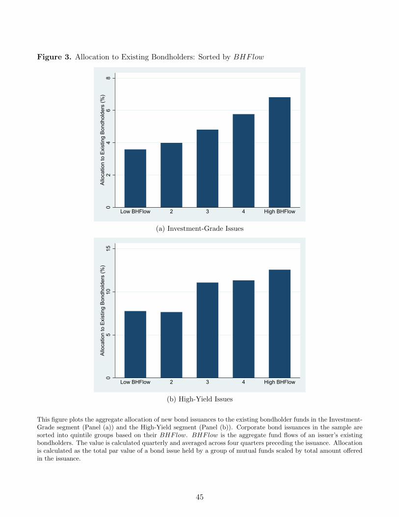
Figure 3. Allocation to Existing Bondholders: Sorted by BHFlow

02

46

8A

lloca

tion

to E

xist

ing

Bon

dhol

ders

(%)

Low BHFlow 2 3 4 High BHFlow

(a) Investment-Grade Issues

05

1015

Allo

catio

n to

Exi

stin

g B

ondh

olde

rs (%

)

Low BHFlow 2 3 4 High BHFlow

(b) High-Yield Issues

This figure plots the aggregate allocation of new bond issuances to the existing bondholder funds in the Investment-Grade segment (Panel (a)) and the High-Yield segment (Panel (b)). Corporate bond issuances in the sample aresorted into quintile groups based on their BHFlow. BHFlow is the aggregate fund flows of an issuer’s existingbondholders. The value is calculated quarterly and averaged across four quarters preceding the issuance. Allocationis calculated as the total par value of a bond issue held by a group of mutual funds scaled by total amount offeredin the issuance.

45

Figure 4. PIMCO’s Fund Flows After Bill Gross’ Departure

-15

-10

-50

5M

onth

ly F

low

(%)

-12 -6 0 6 12 18 24Event Month

Bill Gross Funds Other PIMCO FundsAll Bond Funds

(a) Monthly Flow

-60

-40

-20

0C

umul

ativ

e Fl

ow(%

)

-1 5 11 17 23Event Month

Bill Gross Funds Other PIMCO FundsAll Bond Funds

(b) Cumulative Flow

This figure shows the fund flows for (a) Bill Gross’ Total Return Funds, (b) other funds in the PIMCO fund family,and (c) all bond funds after Bill Gross’ departure from PIMCO in September 2014. Panel (a) exhibits monthlyflows, and Panel (b) exhibits cumulative flows.

46

Figure 5. Issuance Probability of Firms in PIMCO Portfolios After Gross’ Departure

05

1015

20P

roba

bilit

y of

Issu

ance

(%)

2013q1 2014q1 2015q1 2016q1Quarter (Bill Gross Departure = 2014Q3)

Treated (PIMCO) Issuers Control Issuers

This figure displays the probability of new bond issuance for treated firms (PIMCO Issuers) and control firms.Treated issuers are firms whose outstanding bonds were overweighted PIMCO portfolios at the end of 2014Q3 (whenBill Gross left PIMCO). Control issuers are firms whose bonds were held by Prudential or Vanguard portfolios, thesecond and third largest bond managers at the time, for more than 3 percent.

47

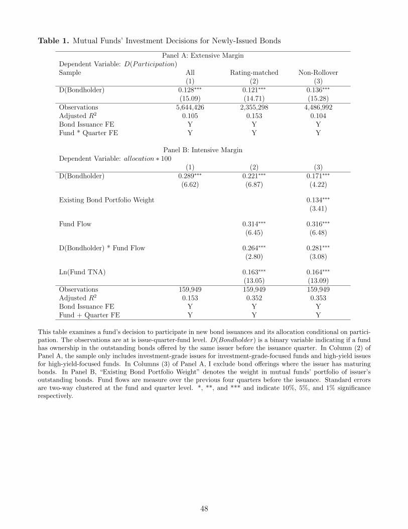
Table 1. Mutual Funds’ Investment Decisions for Newly-Issued Bonds

Panel A: Extensive MarginDependent Variable: D(Participation)Sample All Rating-matched Non-Rollover

(1) (2) (3)D(Bondholder) 0.128∗∗∗ 0.121∗∗∗ 0.136∗∗∗

(15.09) (14.71) (15.28)Observations 5,644,426 2,355,298 4,486,992Adjusted R2 0.105 0.153 0.104Bond Issuance FE Y Y YFund * Quarter FE Y Y Y

Panel B: Intensive MarginDependent Variable: allocation ∗ 100

(1) (2) (3)D(Bondholder) 0.289∗∗∗ 0.221∗∗∗ 0.171∗∗∗

(6.62) (6.87) (4.22)

Existing Bond Portfolio Weight 0.134∗∗∗

(3.41)

Fund Flow 0.314∗∗∗ 0.316∗∗∗

(6.45) (6.48)

D(Bondholder) * Fund Flow 0.264∗∗∗ 0.281∗∗∗

(2.80) (3.08)

Ln(Fund TNA) 0.163∗∗∗ 0.164∗∗∗

(13.05) (13.09)Observations 159,949 159,949 159,949Adjusted R2 0.153 0.352 0.353Bond Issuance FE Y Y YFund + Quarter FE Y Y Y

This table examines a fund’s decision to participate in new bond issuances and its allocation conditional on partici-pation. The observations are at is issue-quarter-fund level. D(Bondholder) is a binary variable indicating if a fundhas ownership in the outstanding bonds offered by the same issuer before the issuance quarter. In Column (2) ofPanel A, the sample only includes investment-grade issues for investment-grade-focused funds and high-yield issuesfor high-yield-focused funds. In Columns (3) of Panel A, I exclude bond offerings where the issuer has maturingbonds. In Panel B, “Existing Bond Portfolio Weight” denotes the weight in mutual funds’ portfolio of issuer’soutstanding bonds. Fund flows are measure over the previous four quarters before the issuance. Standard errorsare two-way clustered at the fund and quarter level. *, **, and *** and indicate 10%, 5%, and 1% significancerespectively.

48

Table 2. Firm-level Summary Statistics

Panel A: Full SampleN Average Std 10th pct Median 90th pct

BHFlow (%) 52,247 1.70 3.47 -1.32 0.78 6.29Bond Issuance Dummy 52,247 0.07 0.26 0 0 0Issuance Amount/Total Assets (%) 52,247 0.66 4.53 0.00 0.00 0.00Market Capitalization ($million) 52,247 12,099 33,522 265 2,842 26,177Total Assets ($million) 52,247 11,461 18,763 666 4,006 31,212Market-to-Book 52,247 1.59 0.84 0.88 1.32 2.67Book Leverage (%) 52,247 31.40 16.27 10.59 30.68 54.08Capital Expenditure (%) 52,247 6.33 5.85 1.38 4.51 13.58R&D Expense (%) 52,247 1.51 3.51 0.00 0.00 4.91Tangibility (% PP&E/Total Assets) 52,247 66.20 39.98 15.58 63.05 120.88Return On Assets (%) 52,247 13.67 6.61 6.26 12.80 22.74Maturing Debt/Total Assets (%) 52,247 3.67 5.85 0.00 1.54 9.54Issuer Investment-Grade Dummy 52,247 0.39 0.49 0 0 1Past 12-Month Stock Return (%) 52,247 14.26 38.76 -33.49 14.62 60.78Past 12-Month Bond Return (%) 52,247 6.61 14.46 -6.23 5.67 19.26BHFlowres (%) 52,247 0.65 2.38 -0.89 0.38 3.58

Panel B: Sorted by BHFlow1(Low) 2 3 4 5(High)

BHFlow (%) -1.51 0.17 1.22 2.59 5.95Bond Issuance Dummy 0.07 0.06 0.06 0.07 0.10Issuance Amount/Total Assets (%) 0.65 0.66 0.62 0.65 0.71Market Capitalization ($million) 9,574 11,235 10,501 13,024 16,132Total Assets ($million) 9,481 11,569 10,543 11,286 14,407Market-to-Book 1.52 1.61 1.63 1.63 1.55Book Leverage (%) 33.56 29.64 29.15 30.62 34.03Capital Expenditure (%) 6.40 6.58 6.44 6.19 6.07R&D Expense (%) 1.21 1.66 1.76 1.57 1.33Tangibility (% PP&E/Total Assets) 66.08 67.56 66.75 65.66 64.96Return On Assets (%) 13.36 13.79 13.79 13.95 13.47Maturing Debt/Total Assets (%) 3.49 3.68 3.57 3.63 3.98Issuer Investment-Grade Dummy 0.32 0.34 0.36 0.46 0.48Past 12-Month Stock Return (%) 14.38 14.88 15.19 13.93 12.94Past 12-Month Bond Return (%) 6.23 6.66 6.70 6.75 6.73BHFlowres(%) 0.14 0.38 0.52 0.88 2.60

This table summarizes bondholder flows and firm characteristics in the main sample. The observations are at thefirm-quarter level. BHFlow is defined in Equation 4, and BHFlowres is defined in Equation 6. Both are measuredcumulatively over the most recent four quarters. In Panel A the full sample is pooled together. In Panel B, firmsare sorted into five group depending on their cross-sectional ranking on BHFlow. The sample period spans from1998 to 2014.

49

Table 3. Bondholder Flow and Firm Bond Issuance Decisions

Dependent Variable: D(Issuancet+1 > 0)Specification Linear Probability Logit Linear Probability Logit

(1) (2) (3) (4) (5) (6) (7) (8)BHFlow (standardized) 0.940∗∗∗ 0.883∗∗∗ 0.812∗∗∗ 0.706∗∗∗

(4.90) (4.94) (3.84) (6.17)

BHFlowres (standardized) 0.656∗∗∗ 0.681∗∗∗ 0.680∗∗∗ 0.655∗∗∗

(3.39) (3.31) (3.52) (4.29)

Ln(Equity Capitalization) 2.459∗∗∗ 2.455∗∗∗ 2.459∗∗∗ 2.318∗∗∗ 2.512∗∗∗ 2.510∗∗∗ 2.509∗∗∗ 2.372∗∗∗

(10.12) (10.36) (10.13) (20.35) (10.13) (10.41) (10.12) (25.05)

Market-to-Book -1.470∗∗∗ -1.132∗∗∗ -1.451∗∗∗ -1.395∗∗∗ -1.521∗∗∗ -1.187∗∗∗ -1.499∗∗∗ -1.425∗∗∗

(-4.99) (-3.95) (-4.97) (-8.17) (-5.20) (-4.16) (-5.17) (-8.70)

Book Leverage -0.0899∗∗∗ -0.0740∗∗∗ -0.0896∗∗∗ -0.0924∗∗∗ -0.0949∗∗∗ -0.0795∗∗∗ -0.0944∗∗∗ -0.0965∗∗∗

(-6.60) (-5.26) (-6.56) (-9.51) (-6.91) (-5.57) (-6.87) (-9.78)

CAPX/Total Assets 0.124∗∗∗ 0.146∗∗∗ 0.123∗∗∗ 0.117∗∗∗ 0.119∗∗∗ 0.142∗∗∗ 0.118∗∗∗ 0.113∗∗∗

(3.55) (3.44) (3.51) (4.99) (3.37) (3.31) (3.34) (4.60)

Asset Tangibility -0.00373 0.00224 -0.00332 -0.00356 -0.00425 0.00209 -0.00383 -0.00394(-0.61) (0.33) (-0.54) (-1.03) (-0.68) (0.30) (-0.61) (-1.14)

Return on Assets 0.0650∗∗ 0.0147 0.0608∗∗ 0.0800∗∗∗ 0.0666∗∗ 0.0161 0.0623∗∗ 0.0836∗∗∗

(2.13) (0.47) (2.01) (3.61) (2.17) (0.51) (2.03) (3.87)

Maturing Debt/Total Assets 0.0900∗∗ 0.125∗∗∗ 0.0892∗∗ 0.0555∗∗∗ 0.0885∗∗ 0.122∗∗∗ 0.0876∗∗ 0.0555∗∗∗

(2.50) (3.64) (2.49) (3.63) (2.46) (3.53) (2.44) (3.60)

Issuer Investment Grade 0.733 0.472 0.809∗∗∗ 0.806 0.544 0.884∗∗∗

(1.30) (0.85) (3.05) (1.40) (0.97) (3.10)

12-Month Issuer Equity Return 0.00375 -0.00105 0.00248 0.00542 0.00363 -0.000979 0.00236 0.00518(1.01) (-0.29) (0.69) (1.57) (0.97) (-0.27) (0.66) (1.49)

12-Month Issuer Bond Return 0.0449∗∗ 0.0394∗∗ 0.0338∗∗ 0.0394∗∗∗ 0.0472∗∗ 0.0415∗∗ 0.0357∗∗ 0.0415∗∗∗

(2.30) (2.04) (2.11) (2.72) (2.43) (2.16) (2.24) (2.84)Observations 52247 52247 52247 52247 52247 52247 52247 52247R2 0.062 0.107 0.065 0.069 0.062 0.106 0.065 0.069Quarter FE Y N/A N/A Y Y N/A N/A YQuarter-by-Industry FE N Y N N N Y N NQuarter-by-IG FE N N Y N N N Y N

This table presents estimates from Equation (7). The observations are at firm-quarter level. BHFlow is definedin Equation 4, and BHFlowres is defined in Equation 6. Both are measured from Quarter t− 3 to Quarter t, andare standardized. All firm characteristics are measured at Quarter t. All columns except Columns (4) and (8) uselinear probability models. Columns (4) and (8) use logit models, and marginal effects evaluated at mean are showninstead of coefficients. All coefficients are multiplied by 100 to ease interpretation. Standard errors are two-wayclustered by issuer and quarter, with the exception of Columns (4) and (8), which are clustered at quarter level. *,**, and *** and indicate 10%, 5%, and 1% significance respectively.

50

Table 4. Bondholder Flow and Bond Offering Yield Spreads

Dependent Variable: Yield Spread (%)(1) (2) (3) (4) (5) (6)

BHFlow (standardized) -0.0555∗∗∗ -0.0510∗∗∗ -0.0443∗

(-2.92) (-2.67) (-1.85)

BHFlowres (standardized) -0.0575∗∗ -0.0402∗ -0.0310∗

(-2.55) (-1.94) (-1.76)

Treasury Yield of Matched Maturity -0.679∗∗∗ -0.722∗∗∗ -0.699∗∗∗ -0.682∗∗∗ -0.683∗∗∗ -0.684∗∗∗

(-10.75) (-11.55) (-10.73) (-10.77) (-10.06) (-10.46)

Merrill Lynch Index Yield of Matched Credit Rating 0.123∗∗∗ 0.0775 0.121∗∗∗ 0.114∗∗

(3.30) (1.66) (3.21) (2.42)

Ln(Equity Capitalization) -0.211∗∗∗ -0.238∗∗∗ -0.191∗∗∗ -0.219∗∗∗ -0.236∗∗∗ -0.330∗∗∗

(-9.22) (-9.74) (-9.27) (-10.04) (-11.85) (-13.01)

Ln(Issue Offering Amount) 0.0813∗∗∗ 0.0968∗∗∗ 0.109∗∗∗ 0.0924∗∗∗ 0.104∗∗∗ 0.141∗∗∗

(3.06) (3.74) (4.02) (3.84) (5.31) (6.90)

Ln(Maturity in Years) 0.268∗∗∗ 0.266∗∗∗ 0.268∗∗∗ 0.271∗∗∗ 0.238∗∗∗ 0.261∗∗∗

(4.86) (4.71) (4.74) (5.06) (3.32) (4.00)

Book Leverage -0.000297 0.00402∗ 0.000789 -0.000514 0.000646 0.00231(-0.16) (1.86) (0.48) (-0.28) (0.33) (1.06)

Return on Assets -0.00621 -0.00307 -0.00241 -0.00623 -0.00683∗ -0.0129∗∗

(-1.59) (-0.60) (-0.64) (-1.59) (-1.80) (-2.76)

Rule 144A 0.131∗ 0.119 0.173∗∗ 0.132∗ 0.0987 0.286∗∗∗

(1.77) (1.31) (2.44) (1.79) (1.26) (4.35)

Credit Rating (numerical) 0.0948∗∗∗ 0.0906∗∗∗ 0.0971∗∗∗ 0.1000∗∗∗

(4.27) (3.48) (4.50) (3.66)

Below A- Grade 0.0862 0.148 0.0721 0.0306(0.98) (1.57) (0.83) (0.30)

Below BBB- Grade 0.772∗∗∗ 0.792∗∗∗ 0.748∗∗∗ 0.758∗∗∗

(6.75) (7.01) (6.81) (7.41)

12-Month Equity Return -0.477∗∗∗ -0.468∗∗∗ -0.442∗∗∗ -0.465∗∗∗ -0.450∗∗∗ -0.361∗∗∗

(-6.19) (-5.71) (-5.54) (-6.10) (-5.75) (-4.25)

Equity Return Volatility 6.146∗∗∗ 5.905∗∗∗ 4.827∗∗∗ 6.077∗∗∗ 5.532∗∗∗ 7.064∗∗∗

(8.51) (6.46) (6.61) (8.49) (7.27) (8.30)

12-Month Issuer Bond Return -0.00728 -0.0103∗∗ 0.00320 -0.00673 -0.00774 -0.00370(-1.46) (-2.37) (0.73) (-1.36) (-1.61) (-0.66)

Observations 5183 5183 5183 5183 5183 5183R2 0.650 0.731 0.725 0.650 0.667 0.644Quarter FE Y N/A N/A Y N/A N/AQuarter-by-Industry FE N Y N N Y NQuarter-by-Rating FE N N Y N N Y

This table presents estimates from Equation (8). The observations are at issuance level. The dependent variable,yield spread, is defined as the difference between bond offering yield and the yield of treasury bills with the closestmaturity. BHFlow is defined in Equation 4, and BHFlowres is defined in Equation 6. Both are measured fromQuarter t− 3 to Quarter t, and are standardized. Rule 144A indicates that the bond issue is privately placed underthe SEC Rule 144A. Credit ratings are measured at bond issue level. Standard errors are two-way clustered byboth issuer and quarter. *, **, and *** and indicate 10%, 5%, and 1% significance respectively.

51

Table 5. Substitution Effects on Equity Issuances and Bank Loans

Panel A: Equity IssuancesDependent Variable: D(EquityIssuet+1 > 0) EquityIssuet+1/TotalAssetst(%)Mean Value: 1.9(%) 0.23(%)Specification Linear Probability OLS

(1) (2) (3) (4) (5) (6)BHFlow (standardized) -0.132∗∗ -0.132∗ -0.137∗∗ -0.0172∗ -0.0250∗∗ -0.0177∗

(-2.04) (-1.95) (-2.17) (-1.73) (-2.22) (-1.97)Observations 52247 52247 52247 52247 52247 52247R2 0.018 0.086 0.020 0.021 0.081 0.022Firm-level Controls Y Y Y Y Y YQuarter FE Y N N Y N NQuarter-by-Industry FE N Y N N Y NQuarter-by-IG FE N N Y N N Y

Panel B: New Term LoansDependent Variable: D(NewLoant+1 > 0) NewLoant+1/TotalAssetst(%)Mean Value: 5.8(%) 0.51(%)Specification Linear Probability OLS

(1) (2) (3) (4) (5) (6)BHFlow (standardized) -0.400∗ -0.452∗ -0.266 -0.0485∗∗ -0.0525∗∗ -0.0362∗∗

(-1.80) (-1.79) (-1.31) (-2.41) (-2.38) (-2.04)Observations 17802 17802 17802 17802 17802 17802R2 0.032 0.168 0.039 0.035 0.171 0.042Firm-level Controls Y Y Y Y Y YQuarter FE Y N N Y N NQuarter-by-Industry FE N Y N N Y NQuarter-by-IG FE N N Y N N Y

This table examines the relation between bondholder flows and equity issuance (Panel A), and bondholder flowsand corporate bank loan initiations (Panel B). BHFlow is defined in Equation 4, and measured from Quarter t− 3to Quarter t. It is standardized to have zero mean and unit standard deviation. In Panel A, the sample containsall bond-issuing firm-quarters as in Table 3. The dependent variable in Columns (1)-(3) is a dummy indicatingif a firm issues equity in Quarter t + 1. The dependent variable is Columns (4)-(6) is a continuous variables ofthe amount of equity issuance scaled by total assets. In Panel B, the sample contains firm-quarters where thefirm has outstanding bonds and has initiated bank loans during the past five years. The dependent variable is anindicator that the firm has a new term loan initiated at Quarter t + 1 (Columns (1)-(3)) or a continuous variableof the amount of newly-initiated bank loans (Columns (4)-(6)). Firm-level control variables include Ln(EquityCapitalization), Market-to-Book Ratio, Book Leverage, Asset Tangibility, Return on Assets, CAPX over TotalAssets, Issuer Investment-Grade Dummy, 12-month Issuer Equity Returns, and 12-month Issuer Bond Returns.All firm characteristics are measured at Quarter t. The coefficients are multiplied by 100 to ease interpretation.Standard errors are two-way clustered by both issuer and quarter. *, **, and *** and indicate 10%, 5%, and 1%significance respectively.

52

Table 6. Use of Issuance Proceeds: Investments, Cash Holdings, and Payouts

Dependent Variable (%) CAPXt

ATt

RnDt

ATt

Acquisitiont

ATt

InvestTotaltATt

∆Casht

ATt

PayouttATt

(1) (2) (3) (4) (5) (6)Issuance Amount 0.143∗∗∗ 0.0507∗∗∗ 0.394∗∗∗ 0.585∗∗∗ 0.119∗∗∗ 0.0438

(4.84) (4.43) (8.58) (14.18) (4.59) (1.35)

D(High BHFlow) * Issuance Amount -0.127∗∗ 0.0239∗ -0.0786 -0.183∗∗∗ 0.0725 0.0687∗

(-2.54) (1.91) (-1.46) (-2.91) (1.60) (1.81)

D(High BHFlow) 0.436 -0.0114 0.572 1.005 -0.413 0.165(0.75) (-0.07) (1.21) (1.64) (-1.30) (0.32)

Ln(Total Assets) -0.411∗∗ 0.345∗∗∗ 0.104 0.0144 0.115 0.836∗∗∗

(-2.29) (8.80) (0.62) (0.07) (1.09) (7.97)Adjusted R2 0.074 0.024 0.124 0.212 0.042 0.097Observations 3512 3512 3512 3512 3512 3512Year FE Y Y Y Y Y Y

This table presents estimates from Equation 11. Issuance Amount is the amount of bond issuance at year t scaledby total assets. D(High BHFlow) is a dummy variable that equals one if BHFlow in year t− 1 is in the highestquartile of the issuance sample. The dependent variables in Columns (1)–(3) are capital expenditure, researchand development costs, and acquisition costs scaled by total assets. In Column (4), the dependent variable is thetotal investment, which is the sum of (1) to (3). In Column (5), the dependent variable is the change in cashholdings. In Column (6), the dependent variable is the equity payout, measured by adding cash dividends andequity repurchases. Standard errors are clustered at the year level. *, **, and *** and indicate 10%, 5%, and 1%significance respectively.

Table 7. Firm characteristics of PIMCO-treated and control firms

Treated Firms Control Firms P (Treated =Control)

Number of Firms 108 278Market Capitalization ($ million) 15,721 16,764 0.80Market-to-Book Ratio 1.65 1.87 0.08Book Leverage (%) 35.6 33.5 0.32Capital Expenditure (%) 5.16 5.56 0.53Asset Tangibility (%) 57.3 58.6 0.78Return on Assets (%) 12.3 14.0 0.02D(Investment-Grade Rating) 0.47 0.51 0.2312-Month Equity Returns (%) 33.39 31.04 0.1612-Month Bond Returns (%) 10.19 9.76 0.49Mautring Debt/Total Assets (%) 2.92 2.93 0.99

This table tabulates the issuer characteristics for the treated and control firms in the PIMCO study. I definetreatment firms as issuers whose bonds have a weight larger than 3% in PIMCO’s portfolios at the end of 2014Q3.The control firms are issuers whose bonds have a weight larger than 3% in Vanguard’s or Prudential’s portfolios.The last column shows the probability under the null that treated firms and control firms have similar characteristicsusing t-tests.

53

Table 8. Bill Gross’ Departure from PIMCO: Impact on Firms’ Bond Issuances

Dependent Variable: Dummy(Issuancet > 0)(1) (2) (3) (4)

Firm in PIMCO*Post Gross Departure -0.0345∗∗ -0.0336∗ -0.0331∗ -0.0348∗∗

(-1.98) (-1.91) (-1.89) (-2.05)

Firm in PIMCO 0.00566 0.0235 0.0229(0.34) (1.52) (1.49)

Post Gross Departure 0.00291 -0.0162(0.35) (-1.44)

6-Month Treasury Yield -0.0331(-0.80)

Treasury 10Y-6M -0.0235(-1.57)

Log(Equity Capitalization) 0.0499∗∗∗ 0.0504∗∗∗ -0.00853(8.22) (8.22) (-0.46)

Market-to-Book -0.00686 -0.00338 0.0777∗∗∗

(-0.47) (-0.23) (2.95)

Book Leverage -0.00126∗∗∗ -0.00133∗∗∗ 0.00439∗∗∗

(-2.60) (-2.75) (4.70)

CAPX/Total Assets 0.00226 0.00251 -0.000387(1.38) (1.52) (-0.11)

Return over Assets 0.00142 0.000991 0.000378(0.95) (0.65) (0.18)

Issuer Investment Grade -0.0167 -0.0165 0.0402(-1.19) (-1.19) (1.15)

12-Month Equity Return -0.0000944 0.00000598 -0.000338(-0.46) (0.03) (-1.41)

12-Month Issuer Bond Return 0.000416 0.000347 0.000682(0.66) (0.43) (0.85)

Observations 5701 5701 5701 5701R2 0.001 0.027 0.031 0.141Quarter FE N N Y YIssuer FE N N N Y

This table shows the results from Equation 12. Firm in PIMCO is an dummy variable that equals one if a firm’soutstanding bonds were overweighted by Pimco’s portfolios at the end of 2014Q3. The control group are firms whoseoutstanding bonds were overweighted by Prudential’s or Vanguard’s portfolios. Post Gross Departure dummy is setto one for quarters between 2014Q4 to 2016Q3, and zero for quarters between 2012Q4 to 2014Q3. The dependentvariable is a dummy variable indicating bond issuance at Quarter t. Standard errors are two-way clustered by bothissuer and quarter. *, **, and *** and indicate 10%, 5%, and 1% significance respectively.

54

Table 9. Mutual Funds’ Investment Decisions for Newly-Issued Bonds: Cross-sectional Variations

Dependent Variable: D(Participation) D(UnderRelation)(1) (2) (3) (4) (5) (6)

D(Bondholder) 0.0552∗∗∗ 0.116∗∗∗ 0.101∗∗∗ 0.121∗∗∗ 0.120∗∗∗ 0.149∗∗∗

(8.11) (15.06) (13.27) (14.40) (14.79) (6.35)

* D(High Yield) 0.153∗∗∗

(11.34)

* D(Shorter Issuance History) 0.0281∗∗∗

(3.75)

* D(Less Analyst Coverage) 0.0649∗∗∗

(8.54)

* D(Fewer Previous Bond Trades) 0.0192∗∗∗

(3.06)

D(UnderRelation) 0.0513∗∗∗

(9.63)Observations 5,644,426 5,644,426 5,644,426 5,644,426 5,644,426 5,644,426Adjusted R2 0.108 0.105 0.106 0.105 0.107 0.027Bond Issuance FE Y Y Y Y Y YFund * Quarter FE Y Y Y Y Y Y

This table examines the cross-sectional variation in mutual funds’ investment decisions as in Equation 13. Theobservations are at is issue-quarter-fund level. D(Participation) is set to one is the mutual fund hold positiveamount of bond at the end of the bond’s issuance quarter. D(UnderRelation) is set to one if a mutual fund hasparticipated in the underwriter’s recent bond issuances. D(Bondholder) is a binary variable indicating if a fundhas ownership in outstanding bonds offered by the same issuer before the issuance. D(High Yield) is an indicatorfor high-yield bonds. D(Shorter Issuance History) is an indicator if a firm has a history of issuing bonds that isshorter than the cross-sectional median. D(Less Analyst Coverage) is an indicator if a firm has fewer-than-mediannumber of analysts covering. D(Fewer Previous Bond Trades) is an indicating if a firm’s outstanding bonds hasfewer-than-median secondary market trading during past quarter. Standard errors are two-way clustered at thefund and quarter level. *, **, and *** and indicate 10%, 5%, and 1% significance respectively.

55

Table 10. Bondholder Flow and Firm Bond Issuance Decisions: Cross-sectional Variations

Dependent Variable: D(Issuancet+1 > 0)(1) (2) (3) (4)

BHFlow (standardized) 0.678∗∗∗ 0.896∗∗∗ 0.481∗∗ 0.444∗

(2.87) (3.49) (2.43) (1.68)

* D(Non-Investment Grade) 0.438∗

(1.83)

* D(Shorter Issuance History) 0.121(0.31)

* D(Less Analyst Coverage) 0.858∗∗

(2.60)

* D(Fewer Previous Bond Trades) 0.750∗∗

(2.41)Firm Characteristics Y Y Y YObservations 52247 52247 52247 52247R2 0.062 0.062 0.063 0.063Quarter FE Y Y Y Y

This table examines the cross-sectional variation in firm bond issuance decisions as in Equation 14. The observationlevel is firm-quarter. BHFlow is defined in Equation 4, and is measured from Quarter t− 3 to Quarter t. D(HighYield) is an indicator for high-yield bonds. D(Shorter Issuance History) is an indicator if a firm has a history ofissuing bonds that is shorter than the cross-sectional median. D(Less Analyst Coverage) is an indicator if a firmhas fewer-than-median number of analysts covering. D(Fewer Previous Bond Trades) is an indicating if a firm’soutstanding bonds has fewer-than-median secondary market trading during past quarter. Other firm characteristicsare the same as in Table 3, and are suppressed from exposition. The coefficients are multiplied by 100 to easeinterpretation. Standard errors are two-way clustered by issuer and quarter. *, **, and *** and indicate 10%, 5%,and 1% significance respectively.

56

Table A1. Determinants of Bond Mutual Fund Flows

Dependent variable: Quarterly Fund FlowsPerformance sorted by 12-Month Raw Returns 12-Month Alphas

(1) (2)Low Performance Rank 0.145∗∗∗ 0.126∗∗∗

(7.68) (5.49)

Mid Performance Rank 0.0199∗∗∗ 0.0355∗∗∗

(3.92) (7.15)

High Performance Rank 0.177∗∗∗ 0.170∗∗∗

(6.81) (6.19)

Average Category Flow 0.741∗∗∗ 0.742∗∗∗

(27.99) (28.14)

Ln(Lagged TNA) -0.00278∗∗∗ -0.00284∗∗∗

(-4.05) (-4.13)

Expense Ratio -1.323∗∗∗ -0.856∗∗∗

(-3.73) (-2.66)

Ln(Fund Age) -0.0381∗∗∗ -0.0376∗∗∗

(-18.57) (-18.31)Observations 181408 181408Adjusted R2 0.126 0.129Quarter FE Y Y

This table examines the determinants of bond mutual fund flows. The observation is at fund-quarter level. Eachquarter, bond funds are ranked by their past 12-month raw returns or alphas and assigned fractional rank Ranki,t−1.I then define “low performance rank” as Min(Ranki,t−1, 0.2), “mid performance rank” as Min(0.6, Ranki,t−1 −Lowi,t−1), and “high performance rank” as Ranki,t−1 − Lowi,t−1 − Midi,t−1. “Average Category Flow” is theaverage flow of funds in the same investment category. Standard errors are two-way clustered at fund and quarterlevel. *, **, and *** and indicate 10%, 5%, and 1% significance respectively.

57