capital structure models - mcmaster university

CAPITAL STRUCTURE MODELS

UNDERSTANDING THE CAPITALSTRUCTURE OF A FIRM THROUGH

MARKET PRICES

By

ZHUOWEI ZHOU, M.SC.

A Thesis

Submitted to the School of Graduate Studies

in Partial Fulfilment of the Requirements

for the Degree

Doctor of Philosophy

McMaster University

c©Copyright by Zhuowei Zhou, 2011.

DOCTOR OF PHILOSOPHY (2011) McMaster University(Financial Mathematics) Hamilton, Ontario

TITLE: UNDERSTANDING THE CAPITAL STRUCTURE OF A FIRM

THROUGH MARKET PRICES

AUTHOR: Zhuowei Zhou,M.SC.(McMaster University)

SUPERVISOR: Dr. Thomas Hurd

NUMBER OF PAGES: xvi, 128

ii

Abstract

The central theme of this thesis is to develop methods of financial mathematics to

understand the dynamics of a firm’s capital structure through observations of market

prices of liquid securities written on the firm. Just as stock prices are a direct measure

of a firm’s equity, other liquidly traded products such as options and credit default

swaps (CDS) should also be indicators of aspects of a firm’s capital structure. We

interpret the prices of these securities as the market’s revelation of a firm’s finan-

cial status. In order not to enter into the complexity of balance sheet anatomy, we

postulate a balance sheet as simple as Asset = Equity + Debt. Using mathemati-

cal models based on the principles of arbitrage pricing theory, we demonstrate that

this reduced picture is rich enough to reproduce CDS term structures and implied

volatility surfaces that are consistent with market observations. Therefore, reverse

engineering applied to market observations provides concise and crucial information

of the capital structure.

Our investigations into capital structure modeling gives rise to an innovative pric-

ing formula for spread options. Existing methods of pricing spread options are not

entirely satisfactory beyond the log-normal model and we introduce a new formula for

general spread option pricing based on Fourier analysis of the payoff function. Our

development, including a flexible and general error analysis, proves the effectiveness

of a fast Fourier transform implementation of the formula for the computation of

spread option prices and Greeks. It is found to be easy to implement, stable, and

applicable in a wide variety of asset pricing models.

iii

Acknowledgements

Needless to say, the list of people in this section is far from being complete.

I would like to thank my thesis advisor Professor Tom Hurd for being a great

mentor and friend. Tom has not only indoctrinated me with financial mathematics

knowledge, but also has taught me to think about problems with passion. His insight

and dedication in this area have been influential to me. Moreover, I really appreciate

the delicious meals amidst our research discussion at his home.

I am also very grateful to Professor Peter Miu and Professor Shui Feng, the mem-

bers of my PHD committee, who have made an enormous commitment to giving me

research suggestions, as well as carefully reading and commenting on my thesis draft.

Their expertise in their own areas has provided me with important supplementary

knowledge. I also would like thank my external examiner Professor Adam Metzler

for carefully reading my thesis and making valuable suggestions.

Many thanks to Professor Matheus Grasselli, Professor David Lozinski, Professor

Roman Viveros-Aguilera and Professor Lonnie Magee for stimulating discussions on

financial mathematics, statistics and econometrics.

I would like to thank participants in the Thematic Program on Quantitative Fi-

nance at Fields Institute in 2010. Communications with them have broadened my

scope in financial mathematics at large and their comments on my presentation in the

6th World Congress of the Bachelier Finance Society have enlightened my subsequent

exploration of the contents in chapter 3 of this thesis in particular.

I also would like to thank the SIAM Journal on Financial Mathematics for issuing

permission license for reprinting my published journal article in chapter 4 of this

thesis. I also appreciate two anonymous referees from the journal, whose valuable

suggestions have led to significant improvements of the article before it was accepted.

Last but not the least, I am indebted to my parents Angen and Yixiang, my wife

Youhai and my new born daughter Mia. Their love and support are my fortune.

iv

Contents

List of Tables viii

List of Figures x

List of Acronyms xiii

Declaration of Academic Achievement xv

1 Background and Motivation 1

1.1 How Good is Mathematical Modeling for Financial Derivatives? . . . 4

1.2 A Filtered Probability Space . . . . . . . . . . . . . . . . . . . . . . . 7

1.3 Literature Review . . . . . . . . . . . . . . . . . . . . . . . . . . . . . 9

1.3.1 Understanding a Firm’s Capital Structure . . . . . . . . . . . 9

1.3.2 Spread Options are Akin to Capital Structure . . . . . . . . . 16

1.4 What Can Be Learnt From This Thesis . . . . . . . . . . . . . . . . . 19

2 Statistical Inference for Time-changed Brownian Motion Credit Risk

Models 22

2.1 Abstract . . . . . . . . . . . . . . . . . . . . . . . . . . . . . . . . . . 22

2.2 Introduction . . . . . . . . . . . . . . . . . . . . . . . . . . . . . . . . 23

2.3 Ford: The Test Dataset . . . . . . . . . . . . . . . . . . . . . . . . . . 25

2.4 The TCBM Credit Setup . . . . . . . . . . . . . . . . . . . . . . . . . 27

2.5 Two TCBM Credit Models . . . . . . . . . . . . . . . . . . . . . . . . 30

2.5.1 The Variance Gamma Model . . . . . . . . . . . . . . . . . . . 30

v

2.5.2 The Exponential Model . . . . . . . . . . . . . . . . . . . . . 30

2.6 Numerical Integration . . . . . . . . . . . . . . . . . . . . . . . . . . 31

2.7 The Statistical Method . . . . . . . . . . . . . . . . . . . . . . . . . . 32

2.8 Approximate Inference . . . . . . . . . . . . . . . . . . . . . . . . . . 36

2.9 Numerical Implementation . . . . . . . . . . . . . . . . . . . . . . . . 40

2.10 Conclusions . . . . . . . . . . . . . . . . . . . . . . . . . . . . . . . . 44

2.11 Additional Material . . . . . . . . . . . . . . . . . . . . . . . . . . . . 48

3 Two-Factor Capital Structure Models for Equity and Credit 54

3.1 Abstract . . . . . . . . . . . . . . . . . . . . . . . . . . . . . . . . . . 54

3.2 Introduction . . . . . . . . . . . . . . . . . . . . . . . . . . . . . . . . 55

3.3 Risk-Neutral Security Valuation . . . . . . . . . . . . . . . . . . . . . 59

3.3.1 Defaultable Bonds and Credit Default Swaps . . . . . . . . . . 60

3.3.2 Equity Derivatives . . . . . . . . . . . . . . . . . . . . . . . . 61

3.4 Geometric Brownian Motion Hybrid Model . . . . . . . . . . . . . . . 62

3.4.1 Stochastic Volatility Model . . . . . . . . . . . . . . . . . . . . 63

3.4.2 Pricing . . . . . . . . . . . . . . . . . . . . . . . . . . . . . . . 64

3.5 Levy Subordinated Brownian Motion Hybrid Models . . . . . . . . . 66

3.6 Calibration of LSBM Models . . . . . . . . . . . . . . . . . . . . . . . 69

3.6.1 Data . . . . . . . . . . . . . . . . . . . . . . . . . . . . . . . . 69

3.6.2 Daily Calibration Method . . . . . . . . . . . . . . . . . . . . 70

3.6.3 Calibration Results . . . . . . . . . . . . . . . . . . . . . . . . 72

3.7 Conclusions . . . . . . . . . . . . . . . . . . . . . . . . . . . . . . . . 74

4 A Fourier Transform Method for Spread Option Pricing 89

4.1 Abstract . . . . . . . . . . . . . . . . . . . . . . . . . . . . . . . . . . 89

4.2 Introduction . . . . . . . . . . . . . . . . . . . . . . . . . . . . . . . . 90

4.3 Three Kinds of Stock Models . . . . . . . . . . . . . . . . . . . . . . 94

4.3.1 The Case of Geometric Brownian Motion . . . . . . . . . . . . 94

4.3.2 Three Factor Stochastic Volatility Model . . . . . . . . . . . . 95

4.3.3 Exponential Levy Models . . . . . . . . . . . . . . . . . . . . 96

vi

4.4 Numerical Integration by Fast Fourier Transform . . . . . . . . . . . 97

4.5 Error Discussion . . . . . . . . . . . . . . . . . . . . . . . . . . . . . 98

4.6 Greeks . . . . . . . . . . . . . . . . . . . . . . . . . . . . . . . . . . . 99

4.7 Numerical Results . . . . . . . . . . . . . . . . . . . . . . . . . . . . . 99

4.8 High Dimensional Basket Options . . . . . . . . . . . . . . . . . . . . 106

4.9 Conclusion . . . . . . . . . . . . . . . . . . . . . . . . . . . . . . . . . 108

4.10 Appendix: Proof of Theorem 9 and Lemma 11 . . . . . . . . . . . . . 109

4.11 Additional Material . . . . . . . . . . . . . . . . . . . . . . . . . . . . 111

5 Summary 113

Bibliography 119

vii

List of Tables

1.1 A simplified and stylized balance sheet for a financial firm (in $ billion). 9

2.1 Parameter estimation results and related statistics for the VG, EXP

and Black-Cox models. Xt derived from (2.23) provide the estimate of

the hidden state variables. The numbers in the brackets are standard

errors. The estimation uses weekly (Wednesday) CDS data from Jan-

uary 4th 2006 to June 30 2010. xstd is the square root of the annualized

quadratic variation of Xt. . . . . . . . . . . . . . . . . . . . . . . . . 41

2.2 Results of the Vuong test for the three models, for dataset 1, dataset 2

and dataset 3. A positive value larger than 1.65 indicates that the row

model is more accurate than the column model with 95% confidence

level. . . . . . . . . . . . . . . . . . . . . . . . . . . . . . . . . . . . . 42


and Black-Cox models using the likelihood function (2.30) in Kalman

filter. The numbers in the brackets are standard errors. The calibration

uses weekly (Wednesday) CDS data from January 4th 2006 to June 30

2010. xstd is the square root of the annualized quadratic variation of Xt. 53


and Black-Cox models. . . . . . . . . . . . . . . . . . . . . . . . . . 78

viii

3.2 Ford accounting asset and debt (in $Bn) reported in the nearest quar-

terly financial statements (June 2010 and March 2011) and estimated

from models on July 14 2010 and February 16 2011. The outstanding

shares of Ford are approximately 3450 MM shares and 3800 MM shares

respectively according to Bloomberg. In the financial statements, we

take the total current assets plus half of the total long-term assets as

the asset, and the current liabilities as the debt. . . . . . . . . . . . . 79

4.1 Benchmark prices for the two-factor GBM model of [32] and relative

errors for the FFT method with different choices of N . The parameter

values are the same as Figure 4.1 except we fix S10 = 100, S20 = 96, u =

40. The interpolation is based on a matrix of prices with discretization

of N = 256 and a polynomial with degree of 8. . . . . . . . . . . . . 104

4.2 Benchmark prices for the 3 factor SV model of [32] and relative errors

for the FFT method with different choices of N . The parameter values

are the same as Figure 4.2 except we fix S10 = 100, S20 = 96, u = 40.

The interpolation is based on a matrix of prices with discretization of

N = 256 and a polynomial with degree of 8. . . . . . . . . . . . . . . 105

4.3 Benchmark prices for the VG model and relative errors for the FFT

method with different choices of N . The parameter values are the

same as Figure 4.3 except we fix S10 = 100, S20 = 96, u = 40. The

interpolation is based on a matrix of prices with discretization of N =

256 and a polynomial with degree of 8. . . . . . . . . . . . . . . . . 106

4.4 The Greeks for the GBM model compared between the FFT method

and the finite difference method. The FFT method uses N = 210 and

u = 40. The finite difference uses a two-point central formula, in which

the displacement is ±1%. Other parameters are the same as Table 4.1

except that we fix the strike K = 4.0 to make the option at-the-money. 107

4.5 Computing time of FFT for a panel of prices. . . . . . . . . . . . . . 107

ix

List of Figures

1.1 Ford’s total asset and debt according to annual financial statements

from 2001 to 2010. . . . . . . . . . . . . . . . . . . . . . . . . . . . . 2

1.2 Ford stock prices after adjustments for dividends and splits from 2001

to 2011. . . . . . . . . . . . . . . . . . . . . . . . . . . . . . . . . . . 4

1.3 Enron historical stock prices in 2001. . . . . . . . . . . . . . . . . . . 11

2.1 The in-sample fit of the two TCBM models and Black-Cox model to

the observed Ford CDS term structure for November 22, 2006 (top),

December 3, 2008 (middle) and February 24, 2010 (bottom). The error

bars are centered at the mid-quote and indicate the size of the bid-ask

spread. . . . . . . . . . . . . . . . . . . . . . . . . . . . . . . . . . . . 45

2.2 Histograms of the relative errors, in units of bid-ask spread, of the in-

sample fit for the VG model (blue bars), EXP model (green bars) and

Black-Cox model (red bars) for dataset 1 (top), dataset 2 (middle) and

dataset 3 (bottom). The tenor on the left is 1-year and on the right,

10-year. . . . . . . . . . . . . . . . . . . . . . . . . . . . . . . . . . . 46

2.3 Filtered values of the unobserved log-leverage ratios Xt versus stock

price for Ford for dataset 1(top), 2 (middle) and 3 (bottom). . . . . 47





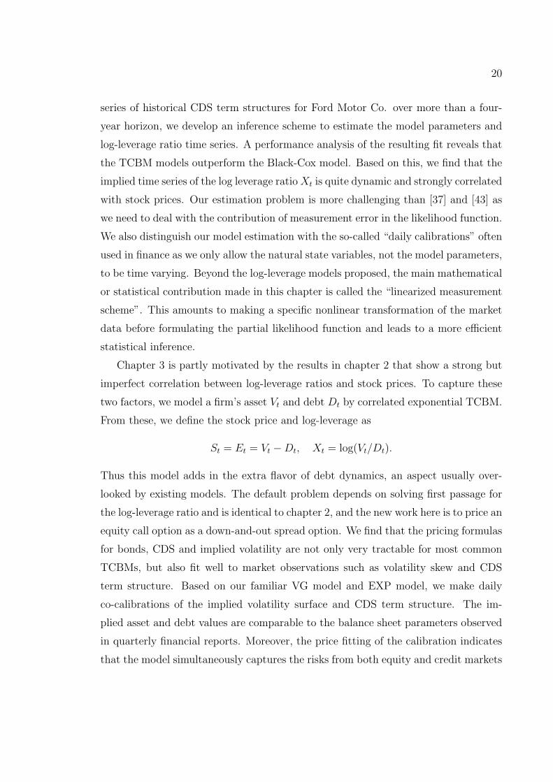
4-year. . . . . . . . . . . . . . . . . . . . . . . . . . . . . . . . . . . . 51

x





7-year. . . . . . . . . . . . . . . . . . . . . . . . . . . . . . . . . . . . 52

3.1 CDS market data (“×”) versus the VG model data (“”) on July 14

2010 (left) and February 16 2011(right). . . . . . . . . . . . . . . . . 77

3.2 Implied volatility market data (“×”) versus the VG model data (“”)

on July 14 2010. . . . . . . . . . . . . . . . . . . . . . . . . . . . . . . 79

3.3 Implied volatility market data (“×”) versus the VG model data (“”)

on February 16 2011. . . . . . . . . . . . . . . . . . . . . . . . . . . . 80

3.4 CDS market data (“×”) versus the EXP model data (“”) on July 14


3.5 Implied volatility market data (“×”) versus the EXP model data (“”)

on July 14 2010. . . . . . . . . . . . . . . . . . . . . . . . . . . . . . . 82

3.6 Implied volatility market data (“×”) versus the EXP model data (“”)

on February 16 2011. . . . . . . . . . . . . . . . . . . . . . . . . . . . 83

3.7 CDS market data (“×”) versus the GBM model data (“”) on July 14


3.8 Implied volatility market data (“×”) versus the GBM model data (“”)

on July 14 2010. . . . . . . . . . . . . . . . . . . . . . . . . . . . . . . 85

3.9 Implied volatility market data (“×”) versus the GBM model data(“”)

on February 16 2011. . . . . . . . . . . . . . . . . . . . . . . . . . . . 86

3.10 CDS spread sensitivities for the EXP model: computed from the 14/07/10

calibrated parameters (solid line), and from setting the log-asset value

v0 one standard deviation (σv) up (dashed line) and down (dash-dotted

line) from the calibration. . . . . . . . . . . . . . . . . . . . . . . . . 87

xi

3.11 Implied volatility sensitivities for the EXP model: computed from the

14/07/10 calibrated parameters (solid line), and from setting the log-

asset value v0 one standard deviation (σv) up (dashed line) and down

(dash-dotted line) from the calibration. . . . . . . . . . . . . . . . . . 88

4.1 This graph shows the objective function Err for the numerical compu-

tation of the GBM spread option versus the benchmark. Errors are

plotted against the grid size for different choices of u. The parameter

values are taken from [32]: r = 0.1, T = 1.0, ρ = 0.5, δ1 = 0.05, σ1 =

0.2, δ2 = 0.05, σ2 = 0.1. . . . . . . . . . . . . . . . . . . . . . . . . . 101


tation of the SV spread option versus the benchmark computed using

the FFT method itself with parameters N = 212 and u = 80. The

parameter values are taken from [32]: r = 0.1, T = 1.0, ρ = 0.5, δ1 =

0.05, σ1 = 1.0, ρ1 = −0.5, δ2 = 0.05, σ2 = 0.5, ρ2 = 0.25, v0 = 0.04, κ =

1.0, µ = 0.04, σv = 0.05. . . . . . . . . . . . . . . . . . . . . . . . . . 102

4.3 This graph shows the objective function Err for the numerical com-

putation of the VG spread option versus the benchmark values com-

puted with a three dimensional integration. Errors are plotted against

the grid size for five different choices of u. The parameters are: r =

0.1, T = 1.0, ρ = 0.5, a+ = 20.4499, a− = 24.4499, α = 0.4, λ = 10. . . 103


tation of the SV spread option versus the benchmark computed using

1, 000, 000 simulations, each consisting of 2000 time steps. The pa-

rameter values are taken from [32]: r = 0.1, T = 1.0, ρ = 0.5, δ1 =

0.05, σ1 = 1.0, ρ1 = −0.5, δ2 = 0.05, σ2 = 0.5, ρ2 = 0.25, v0 = 0.04, κ =

1.0, µ = 0.04, σv = 0.05. . . . . . . . . . . . . . . . . . . . . . . . . . 112

xii

List of Acronyms

APT Arbitrage Pricing Theory

BC Black-Cox

BDLP Background Driving Levy Processes

BIS Bank for International Settlements

BK Black-Karasinski

BMO Bank of Montreal

CDF Cumulative Density Function

CDO Collateralized Debt Obligation

CDS Credit Default Swap

CLO Collateralized Loan Obligation

CMS Constant Maturity Swap

CVA Credit Valuation Adjustment

DtD Distance-to-Default

EAD Exposure at Default

EC Economic Capital

EMM Equivalent Martingale Measure

EXP Exponential

FP First Passage

FFT Fast Fourier Transform

FX Foreign Exchange

GBM Geometric Brownian Motion

GCorr Global Correlation

IID Independent Identical Distribution

ITM In-the-Money

IV Implied Volatility

KF Kalman Filter

xiii

LGD Loss Given Default

LOC Line of Credit

LSBM Levy Subordinated Brownian Motion

MBS Mortgage-Backed Security

MKMV Moody’s KMV

MLE Maximum Likelihood Estimation

MtM Mark-to-Market

NYSE New York Stock Exchange

OTC Over-the-Counter

OTM Out-of-the-Money

PD Default Probability

PDE Partial Differential Equation

PDF Probability Density Function

PIDE Partial Integro-Differential Equation

RBC Royal Bank of Canada

RMSE Root Mean Squared Error

RV Realized Variance

SEA Self-Exciting Affine

SD Structural Default

S & P Standard & Poor’s

SV Stochastic Volatility

TCBM Time-Changed Brownian Motion

TTM Time to Maturity

UAW United Auto Workers

VG Variance Gamma

xiv

Declaration of Academic Achievement

My “sandwich thesis” includes three self-contained and related financial mathe-

matics papers completed during my PhD study from 2007 to 2011.

The first paper “Statistical Inference for Time-changed Brownian Motion Credit

Risk Models” in chapter 2 has been submitted for peer review [60] in early 2011.

This paper demonstrates how common statistical inference, in particular maximum

likelihood estimation (MLE) and Kalman filter (KF) can be efficiently implemented

for a new class of credit risk models introduced by Hurd [57]. For this class of models,

traditional estimation methods face challenges such as computational cost due to a

non-explicit probability density function (PDF). My coauthor Professor Hurd and I

have made significant improvement on resolving these issues and a study on Ford

Motor Co. historical data shows our new method is fast and reliable. Professor Hurd

and I are both equal contributors in the writing of this paper. More specifically I

have made the following contributions: 1. Numerous studies leading to the statistical

solution as the core of the paper including alternative approaches; 2. Most of the

technical aspects of this paper, including mathematical derivations, data collection,

computer programming and numerical analysis; 3. An equal share of drafting and

finalizing of the paper.

The second paper “Two-Factor Capital Structure Models for Equity and Credit”

in chapter 3 is ready to be submitted for peer review [61]. This paper extends the

classical Black-Cox (BC) model in credit risk to a model of the capital structure of

a firm that incorporates both credit risk and equity risk. In contrast to other exten-

sions to the BC model that are restricted by a one-factor and/or diffusive nature, our

model contains a two-factor characterization of firm asset and debt, and allows their

dynamics to diffuse and jump. With much greater flexibility, our model retains sat-

isfactory tractability and important financial derivatives can be priced by numerical

integrations. We demonstrate the strength of the model by showing its improved fit

xv

to market data. My coauthor Professor Hurd and I are both equal contributors in

the writing of this paper. More specifically I have made the following contributions:

1. An equal share of the original idea of this paper that evolved from our discussions;

2. Most of the technical aspects of this paper, including mathematical derivations,

data collection, computer programming and numerical analysis; 3. An equal share of

drafting and finalizing of the paper.

The third paper “A Fourier Transform Method for Spread Option Pricing” in

chapter 4 has been published in the SIAM Journal of Financial Mathematics [59]1.

This paper introduces a new formula for general spread option pricing based on

Fourier analysis of the payoff function. This method is found to be easy to implement,

stable, efficient and applicable in a wide variety of asset pricing models. On the

other hand, most existing tractable methods are not entirely satisfactory beyond the

log-normal model. Few exceptions are either computationally costly or subject to

unsatisfactory numerical errors. My coauthor Professor Hurd and I are both equal

contributors in the writing of this paper. More specifically I have made the following

contributions: 1. Setting up the theoretical framework; 2. Most of the technical

aspects of this paper, including mathematical derivations, computer programming

and numerical analysis; 3. An equal share of drafting and finalizing of the paper.

1Copyright c© 2010 Society for Industrial and Applied Mathematics. Reprinted with permission.

All rights reserved.

xvi

Chapter 1

Background and Motivation

In the private sector, a firm finances its assets through a combination of equity,

debt, or hybrid securities, leaving itself liable to various financial stakeholders. The

composition or “structure” of these liabilities makes up its capital structure. A de-

tailed capital structure tells rich information about a firm, such as its creditworthiness,

its access to financing options, and even regulatory restrictions on the firm.

The management of a firm knows its capital structure well enough to make strate-

gies that help the firm grow. Outsiders, such as rating agencies and stakeholders, need

to know capital structure better to make forecasts of the firm. Balance sheets unveiled

in quarterly financial statements provide a good snapshot of the capital structure to

the public. However, balance sheets are inconvenient for real-time analysis as they

are not available between reporting dates. Their relevance can also be obscured by

accounting specifics and time delay. In addition, investors usually gather information

from a firm’s issued securities. For example, equity dilution can lead to the stock

price dropping, while debt restructuring can lead to a slashing of bond prices. How-

ever, such analyses are ad hoc and intuitive, and they are difficult to extend to more

quantitative problems.

We believe financial mathematics is a more sophisticated tool that can reveal

non-intuitive and in-depth connections between market prices and a firm’s capital

structure. Its advantages are mainly two fold. First of all, by replacing a real world

problem by a mathematical model one focuses critical attention on the underlying

1

2

idealizing assumptions. Once the assumptions have been accepted the rules of math-

ematics lead to clear results that can improve intuition. Also, mathematical modeling

can simplify each problem by retaining only key factors and omitting others. For ex-

ample, in our models we postulate a balance sheet as simple as Asset = Debt+Equity,

which we write as

Vt = Dt + Et (1.1)

for each time t. Second of all, it is flexible and can take as inputs a broad spectrum

of market prices. In addition to the “baseline” cases of stocks and bonds, one can

include liquidly traded financial derivatives such as options, credit default swaps

(CDS), which should also be indicators of aspects of a firm’s capital structure. The

values of capital structure can be learnt by comparing or calibrating model prices to

these market prices.

Figure 1.1: Ford’s total asset and debt according to annual financial statements from

2001 to 2010.

While financial mathematics provides alternatives to understand a firm’s capital

structure, a caveat needs to be mentioned. The model implied capital structure

represents market values of asset, debt etc. in a “mark-to-market” (MtM) sense,

3

as are the traded instruments used for calibration. However, the capital structure

in a balance sheet represents accounting values that are calculated and interpreted

differently [105]. So it is not important for us to reproduce the accounting balance

sheet or even to obtain a capital structure similar to it. Instead, our aim is to provide

an independent measure of the capital structure implied from market prices. To

illustrate this point, we see from figure 1.1 that Ford’s accounting V − D became

negative for several years which is impossible in our MtM calibration.

The value of any model can only be fully realized in real life applications. Admit-

tedly, there are numerous firms worthy of detailed case study and in this thesis we

chose one firm that is of particular interest. Ford Motor Company (NYSE: F) is the

second largest automaker in the US and was the fifth largest in the world based on an-

nual vehicle sales in 2010. It is the eighth-ranked overall American-based company in

the 2010 Fortune 500 list, based on global revenues in 2009 of $118.3 billion. However,

this giant name in the global auto industry really stumbled in the last decade. As a

result of declining market share, corporate bond rating agencies had downgraded the

bonds of Ford to junk status by 2005. In 2006 in the wake of a labor agreement with

the United Auto Workers (UAW), the automaker reported the largest annual loss in

company history of $12.7 billion. At the peak of the financial crisis, Ford announced

a $14.6 billion annual loss, making 2008 its worst year in history.

We note that Ford Motor Company experienced a large number of credit rating

changes during this period. The history of Standard & Poor’s (S & P) ratings is as

follows: A to BBB+ on October 15, 2001; BBB+ to BBB on October 25, 2002; BBB

to BBB- on November 12, 2003; BBB- to BB+ on May 5, 2005; BB+ to BB- on

January 5, 2006; BB- to B+ on June 28, 2006; B+ to B on September 19, 2006; B to

B- on July 31, 2008; B- to CCC+ on November 20, 2008. The downgrades continued

into 2009, with a move from CCC+ to CC on March 4, 2009 and to SD (“structural

default”) on April 6, 2009. The latest news was improving: on April 13, 2009, S &

P raised Ford’s rating back to CCC, on November 3, 2009 to B-, and on August 2,

2010 to B+, the highest since the onset of the credit crisis. On February 2, 2011, it

rose to BB-.

In hindsight we see that Ford never actually defaulted during this period, although

4

Figure 1.2: Ford stock prices after adjustments for dividends and splits from 2001 to

2011.

it came close. It implies that this company stays solvent in the MtM sense as its

asset has a narrow margin over debt. From market prices, we not only see that its

stock volatility and CDS have been priced high, but also that they evolved quite

dynamically. It is therefore of particular interest to use Ford as a case study in this

thesis to understand how much market prices tell about its capital structure.

1.1 How Good is Mathematical Modeling for Fi-

nancial Derivatives?

In financial markets, a derivative is a security whose value depends on other,

more basic, underlying variables [53]. The global financial derivative markets have

seen staggering growth during the last two decades. According to the Bank for

International Settlements (BIS) in March 2011 [9] the notional outstanding amounts

of Over-the-Counter (OTC) derivatives reached $583 trillion with gross market values

of $25 trillion in June 2010. The notional outstanding amounts of exchange traded

5

derivatives reached $78 trillion in December 2010.

Paralleling the burgeoning in market size has been financial innovation. Market

makers who provide financial market liquidity have tailored existing derivatives or

invented entirely new ones to meet customers’ financial needs. For example, variance

swaps [21] provide investors with opportunities to hedge and speculate on market

volatilities. Credit Default Swap (CDS) contracts provide investors with default pro-

tection on sovereign, municipal and corporate bonds. The highest profile innovation of

Wall Street is probably securitization, among the associated securities are so-called

structured instruments such as Mortgage-Backed Securities (MBS), Collateralized

Loan Obligations (CLO) and Collateralized Debt Obligations (CDO). These instru-

ments attract capital from international investors to provide less costly funding in

otherwise illiquid housing markets, loan markets and speculative bond markets. For

example, the CDO issuance grew from an estimated $20 billion in Q1 2004 to its peak

of over $180 billion by Q1 2007 [101], while the numbers for MBS are even greater

[88].

Even if intended as a way to off-load or manage risk, such complex derivatives may

also harm holders with unexpected risks. Warren Buffett famously called derivatives

“financial weapons of mass destruction”, which illuminates the risky side of deriva-

tives. Narrowly speaking, because of leverage, a trader could lose everything in option

trading with only a modest movement of the underlying stock. From a global per-

spective, the 2007-2010 financial crisis (for a description of the crisis see [51] and

its references therein) would have been contained within the housing market where

it originated if complex derivatives such as MBS, MBS CDO had not become so

widespread (See [51][52]). The subprime mortgage market only amounted to a small

part of the US economy or even of the prime mortgage market. However, its impact

swiftly propagated into US capital markets and eventually eroded the global econ-

omy. Among many other causes of the crisis is OTC derivatives’ role in transferring

risks, that can lead to systemic risks (See [28] for a good illustration of so-called con-

tagion and systemic risks). A panacea might be to go back to the old, simple days

when there was no room for complex, toxic securities. However, this view misses the

fact that complex derivatives serve the same primary purpose as stocks and bonds,

6

in a more sophisticated way, to direct limited resources (funding) to promote social

development. The technology of risk pooling and risk transfer has been an essential

component of capital markets for centuries, with innovations that have arisen in re-

sponse to legitimate needs of individuals and corporations. Their real benefits are

the basis for people’s good faith on them.

Until recently, market participants have been content to use the modern mathe-

matical finance theory, pioneered by Black, Scholes and Merton in the 1970s [11][85][106],

to hedge and price derivatives. Experienced traders make estimates of their bid/ask

prices starting from the bare-bones model prices. They also quantify their risk expo-

sures in terms of model dependent risk metrics such as Greeks. During the financial

crisis people have seen the predictions of financial models diverge dramatically from

empirical observations, and consequently much criticism has been cast on quantitative

modeling in general, and sometimes even a particular formula [94][102]. The basis

of this negative voice is that quantitative analysts (“quants”) failed to build “right”

models to capture dangerous risks that ultimately pushed the financial system to the

brink. To provide an opposite view, several renowned researchers wrote on this sub-

ject in their columns or papers [36][77][100][107]. These authors contrasted financial

models with physics models and illustrated why financial models have yet to achieve

the level of accomplishment of physics models. In Lo and Mueller’s Taxonomy [77],

physics has been very successful in modeling a world with “complete certainty” and

“risk without uncertainty”. This physics world involves deterministic motions such

as planetary orbits and harmonic oscillation and controlled lab experiments such as

atomic collisions and crystal growth. In contrast, financial models must cope with

the mental world of monetary value. They aim at reducing humans’ irreversible and

unrepeatable behavior to a simplified mechanism. Modeling this realm of “partially

reducible uncertainty” is a much more ambitious undertaking than physics. There

is no “right” model because the world changes in response to the models we use

1. On the other hand, there is the “right” use of models. In the course of modern

mathematical finance theory, models are developed that work for different markets

1Take arbitrage trading for example. Arbitrage trading always annihilates existing arbitrage

opportunities. So the same trading algorithms would fail after short-term usage.

7

under different scenarios, to maximize their utility and accuracy. There are some best

available models for specific finance or economics problems. The right use of models

also requires users’ good judgment. As Steve Shreve put it [100], . . . a good quant also

needs good judgment. A wise quant takes to heart Albert Einstein’s words, “As far as

the laws of mathematics refer to reality, they are not certain; and as far as they are

certain, they do not refer to reality. . . ”. The right use of models involves much more

than finding a generic model that works for all.

This thesis presents mathematical models of capital structure that are more robust

and have weaker assumptions than some existing ones. Our aim will be to show that

these models work reasonably well in the markets we investigated. We also provide

mathematical techniques that make these models tractable and therefore be applied

to real industry problems. We hope that these works will complement and extend

the current financial literature and provide new tools to improve risk management of

the financial markets.

1.2 A Filtered Probability Space

In modern mathematical finance theory, underlying dynamic market variables are

modeled as stochastic processes. The probabilistic specifications of these selected

stochastic processes must reflect empirical market observations to diminish the so-

called “model risk”. On top of these processes, there is a filtered probability space

(Ω,F ,Ft,Q) that formalizes their evolution with respect to time. Here Ω is a non-

empty set that includes all possible “outcomes” or realizations of the underlying

stochastic processes and F is a σ−algebra of subsets of Ω. With the calendar time

starting from 0 and denoted by t, the filtration (Ft, t ≥ 0) is a family of sub σ−algebras

of F such that Fs ⊆ Fq whenever s ≤ q. Each subset A in F is called an event, and

its probability of occurrence is given by the probability measure Q(A). It is naturally

required that Q(A) ≥ 0 and Q(Ω) = 1.

It is standard in probability theory to require some further conditions on a filtra-

tion, and the following pair of conditions are referred as the usual hypotheses:

8

• (completeness) F0 contains all sets of Q−measure zero;

• (right continuity) Ft = Ft+ where Ft+ = ∩ε>0Ft+ε.

Let the underlying stochastic process X = (X(t), t ≥ 0) be a mapping from

R+ to Rd. We say that it is adapted to the filtration (or Ft−adapted) if X(t) is

Ft−measurable for each t ≥ 0. Any process X is adapted to its own filtration

FXt = σX(s); 0 ≤ s ≤ t and this is usually called the natural filtration.

In mathematical finance modeling, the filtration is intimately connected to the

information revealed by the market at a time on-going basis. The most accessible

information is given by the “market filtration” Gt ⊂ Ft defined by the market observ-

ables. Hidden variables such as the short rate and stochastic volatilities are adapted

to hidden filtrations that may or may not be “backed out” from observables such as

traded options. When some investors gain access to a larger filtration, either from

superior information channels or better modeling, they may be able to create a so-

called dynamic arbitrage [19] to risklessly cash-out at the expense of others. In this

thesis, we work with probability space. Our market observables include stock prices,

implied volatility (IV) surfaces and CDS term structures that are made available to

the public. In addition, our models have a small dimensional family of hidden Markov

variables, or latent variables that includes firm asset, debt and leverage ratio. Infer-

ence of these hidden values is made from traded securities on the firm, and possibly

its balance sheets as well.

For formal descriptions of probability theory and stochastic processes, one can

refer to standard probability textbooks such as [3] and [65]. [99] also provides math-

ematical finance interpretations of probability theory.

9

1.3 Literature Review

1.3.1 Understanding a Firm’s Capital Structure

Balance Sheet Analysis

The straightforward way to understand a firm’s capital structure is to read off

its balance sheet from published quarterly financial statements. In a simplified and

stylized balance sheet, a firm’s capital structure consists of assets and an equal (“bal-

anced”) amount of liabilities that consist of shareholders’ equity and debt holders’

debt 2. Table 1.1 illustrates a simplified balance sheet. In this case, a financial firm is

funded by $10 billion from equity holders and $90 billion from debt holders, the total

of which is invested in assets which are mostly securities. If we define the leverage

ratio as the ratio of asset over debt 3, the firm’s leverage ratio is 109

. Typically, a

standard balance sheet in financial accounting further breaks down assets into cur-

rent assets and non-current assets, debt into short term current debt and long term

non-current debt, equity into paid-in capital and retained earnings etc. [105]. A de-

tailed balance sheet is very useful for static performance analysis of a firm. Altman [1]

used seven quantities in a balance sheet to calculate the famous Z-score to determine

firms’ survivability. Rating agencies rely heavily on balance sheets to estimate the

default probability (PD), exposure at default (EAD) and loss given default (LGD) of

different bonds issued by a firm.

Assets Liabilities

Securities, 100 Debt, 90Equity, 10

Table 1.1: A simplified and stylized balance sheet for a financial firm (in $ billion).

2In many occasions, liabilities are used to represent debt exclusively. Our definition of liabilities

stresses that a firm is also liable to equity holders.3In financial accounting, leverage ratio of a firm is usually defined as the ratio of debt over asset

or debt over equity. We use this definition to conform to the log leverage ratio Xt = log(Vt/Dt) in

chapter 2.

10

The Collapse of Enron

The demise of the giant energy corporation Enron was the highest profile bankruptcy

reorganization in American history up to that time. Its quick fall a couple of months

after its first quarterly loss report in years shocked investors and auditors:

• Enron headed into 2001 with a stock price of about $80. On June 19, Jeffrey

Skilling, the incumbent chief executive officer, reiterated “strong confidence” in

Enron’s earning guidance to investors. On the same day, Enron’s daily realized

variance (RV) jumped dramatically from 66 percent to 158 percent.

• On August 14, Skilling resigned unexpectedly, triggering Wall Street’s concern

about Enron’s real financial status. The equity price fell from $42.93 to $36.85

in two days. Daily RV increased from 29 percent on August 13 to 84 percent

and 131 percent on August 14 and 15 respectively.

• On October 16, Enron’s first quarterly loss in more than four years was made

public through its financial statement, accompanied by a $1.2 billion charge

against shareholders’ equity. Its equity price dropped from $33.84 to $20.65 in

the next four days. Daily RV moved up into the range of 85-210 percent.

• On November 8, Enron announced that it would restate its earnings from 1997

through 2001, which further brought down its equity to $8.63 during that week.

Daily RV reached 262 percent.

• On November 28, credit-rating agencies downgraded Enron’s bonds to junk

status, and Enron temporarily suspended all payments before filing for Chapter

11 bankruptcy protection on December 2. The daily RV experienced its highest

spike of 1027 percent.

From the Enron case, we can see that infrequently published balance sheet information

does not fit well with a dynamic analysis of capital structure, especially for short term,

since apart from the share value, balance sheet entries are only available quarterly and

with time delay. The main theme of this thesis is to explore an alternative, namely

11

Figure 1.3: Enron historical stock prices in 2001.

to deduce a simplified capital structure from prices of market observables which are

more abundant and reliable, using tractable mathematical finance models.

Structural Approach in Credit Modeling

The structural approach to credit risk models balance sheet parameters of a firm

such as asset, debt or leverage as underlying processes, and treats securities issued

by the firm such as bonds and stock as contingent claims on the firm’s assets. This

stream of modeling begins with the seminal works of Merton [86] and Black and Cox

[10], in which they assumed a geometric Brownian motion (GBM) for the firm asset

process and modeled the firm default as the time the asset value hits a continuous

or discrete barrier equal to the debt value. While Merton assumed default can only

happen at a bond maturity, Black and Cox made default a first passage (FP) event

that can happen any time within the maturity horizon. Because its first passage

concept in credit modeling is used throughout this thesis, we now outline the Black-

Cox framework. We work in a filtered probability space (Ω,F ,Ft,Q), where Ft is

the natural filtration of a Brownian motion Wt and Q is the risk-neutral measure.

12

In such a probability space, the total value Vt of a firm’s assets follow a geometric

Brownian motiondVtVt

= (µ− δ)dt+ σdWt (1.2)

where µ is the mean rate of return on the asset, δ is a proportional cash pay-out rate

and σ is the volatility. The firm’s capital structure includes a single outstanding debt

with a deterministic value Dt, which has a maturity T and face value DT = D. Black

and Cox postulated that default occurs at the first time that the firm’s asset value

drops below the debt value. That is, the default time is given by

τ = inft > 0 : Vt < Dt (1.3)

This is a simplification of the notion of a safety covenant in corporate finance which

gives debt holders legal rights to force liquidation of the asset of a firm if it fails to

service any coupon or par obligations. Consistent with the limited liability for equity

holders, the pay-off for equity holders at maturity is

(VT −DT )+1τ>T (1.4)

A natural choice of the debt value process assumes a constant growth rate k ≥ 0

so Dt = De−k(T−t) which leads to an explicit formula for the density function of τ as

well as a formula for the value of equity.

Beyond the Merton and Black-Cox Models

Along the lines of Merton and Black-Cox, there have been various extended ver-

sions in credit risk modeling. Hull and White [55] revised the Black-Cox model by

using piecewise constant default barriers and were able to fit perfectly a given term

structure of default rates derived from market CDS rates. Nielsen et.al. [91], Briys

et.al. [15], and Schobel [96] modeled stochastic interest rates that brought random-

ness to the default boundary. Leland [72], Leland and Toft [73], and Mella-Barral

and Perraudin [83] considered strategic default which is exercised by a firm’s man-

agement (i.e. the equity holders) to maximize its equity value. Vendor’s software,

such as Moody’s KMV (MKMV) [30], stemmed from the Merton model. Rather than

13

looking at asset and debt individually, Moody’s KMV models its proprietary account-

ing ratio called distance-to-default (DtD) that serves as a normalized measure of the

margin between the asset and debt. Other authors have incorporated more financial

intuition into the definition of default. Cetin et.al. [27] defined default as the time

when a firm’s cash balance hits a secondary barrier after staying below the primary

barrier of zero (financial stress) for an extended period of time. Yildirim [108] defined

default as the first time the firm value stays under a barrier for an extended period

measured by the integral of the firm value with respect to time. The financial im-

plication is that when a firm becomes financially stressed, it still has some chance of

revival by accessing liquidity or bank lines of credit (LOC) before default is triggered.

The performance of several structural models has been tested by Eom et.al.[42].

While the Merton and Black-Cox models have been widely accepted due to their

consistency with financial intuition and tractability in mathematical treatment, their

shortcomings are also well known. They predict that term structures of credit spreads

must have a zero short spread and a particular hump shape that is unrealistic. At least

for investment grade credits there is evidence against humps and for increasing credit

spreads [76][95][50]. Moreover, the Merton model has a time inconsistency problem

when it comes to derive the PD term structure. For more detailed discussion of these

models, one can refer to standard credit risk books for example [39][69][97].

Within the structural approach the majority of works that succeed in producing

flexible term structures start from one of two fundamental ideas:

1. Introduce jumps into the firm asset, debt or leverage ratio processes so that the

creditworthiness of a firm can have a good opportunity for a substantial move

in a short period of time, making default an “unpredictable” event. Various

numerical methods have been developed to improve tractability. Zhou [111] is

the first to use Monte Carlo simulation in this kind of structural models to make

the connection between jumps and non-zero short spread. Kou and Wang [68]

used Kou’s earlier asset price model and took advantage of the “memoriless”

feature of the exponential jumps to derive an explicit Laplace transform of the

first passage time, leading to the formulas for the first passage time density and

14

credit spreads involving Laplace inversion [8]. More generally, the Wiener-Hopf

factorization gives the Laplace transform of the joint characteristic function of

a Levy process and its running maximum, and has been used to price barrier

options under Levy processes [29]. Similarly, it can be used to calculate the

first passage time density in the structural approach. Moreover, a first passage

time of the second kind invented by Hurd [57] has a semi-closed form density

function in terms of a spectral expansion for a broad class of time changed

Brownian motions (TCBM), so that credit spreads can be efficiently calculated

by one dimensional numerical integrations.

2. Introduce uncertainties into the current observation of a firm’s asset or debt

so that the firm’s default event becomes unpredictable. Duffie and Lando [38]

assumed that a firm’s asset is observed with accounting noises, only at certain

points in time. Giesecke [46] assumed that a firm’s default threshold has some

prior distribution known to investors, and which can be updated with new

information from bond markets. In the vendor software CreditGrades [45], the

default threshold is a log-normally distributed random variable drawn at time

zero.

There are several notable merits of the structural approach. First of all, it has

a clear economic interpretation. The framework links balance sheet parameters of

asset and debt to the market tradable stocks and bonds, and is consistent with arbi-

trage pricing theory (APT). People have been able to implement reverse engineering

of structural models using readily available equity and bond data to estimate unob-

served asset and debt values of a firm. In Bensoussan et.al [7], the asset volatility of a

firm is analytically derived from the equity volatility. The interpretation of the lever-

age effect in equity markets is also addressed. Duan [37] and Ericsson and Reneby

[43] used maximum-likelihood estimation (MLE) to obtain a firm’s asset value from

equity data. The best-known vendor software of this kind Moody’s KMV uses a

proprietary structural approach 4 to estimate time series of asset values for a vast

4Moody’s KMV is (understandably) reluctant to release all details of the model as they are trying

to sell the model.

15

pool of public firms in its database. Its “GCorr” (Global Correlation) model provides

asset correlation matrices calculated from these time series. Very recently, Eberlein

and Madan [41] went further to use both traded equity options and balance sheet

statements to evaluate a firm’s impact on the economy. They argued that limited

liability applies to all of a firm’s stakeholders not just the shareholders, and claimed

the shortfall amounted to a “taxpayer put” option written by the economy at large.

They model both a firm’s risky assets and debts as exponential Levy processes. After

calibration to balance sheet statements and equity options for six US banks, their

model is able to put a value on these taxpayer put options and an acceptable level of

capital reserves.

Second of all, the structural approach is naturally suited to analyze one type of

relative value strategy commonly used in hedge funds and investment banks, namely

capital structure arbitrage[109]. Capital structural arbitrage relies on model depen-

dent links between seemingly unrelated securities of the same firm and explains secu-

rity prices inconsistent relative to others as mispricing by the market. The statistical

arbitrage profits by investing in expectation that this mispricing eventually vanishes,

forced by the fundamental value of the firm. Built on a structural model, Cred-

itGrades is an industry benchmark model for evaluating CDS prices from a firm’s

current share price, historical equity volatility, debt per share, historical recovery

rate and model assumptions. Yu [110] used CreditGrades to study possible arbitrage

opportunities achievable by trading on the relative values of equity and CDS.

Third of all, the structural approach allows for flexible asset and default corre-

lation. For pure diffusive processes, correlation of names can be parameterized in

a correlation matrix and for a large portfolio one can introduce factor models in

which correlations are parameterized by a reduced number of factor loadings. The

popularity of the structural approach has reached various multi-name problems, such

as economic capital (EC)[30][47], credit valuation adjustment (CVA)[55][14][12][75],

CDO pricing [56][54]. Due to the fact that a broad class of Levy processes is subor-

dinated Brownian motion [57][29], some far-reaching research has studied correlation

for this class of Levy processes.

In spite of the success of the structural approach, one should always recall a

16

line of caveat in its usage. No direct correspondence of the market value of asset,

debt or leverage to a firm’s balance sheet parameters is necessary for the validity

of this approach: all that matters is that there are such processes (observable or

unobservable), and that they indicate the creditworthiness of the firm.

1.3.2 Spread Options are Akin to Capital Structure

The stylized balance sheet (1.1) can be written Et = Vt−Dt. This implies that an

equity option is akin to a spread option, and it suggests that one can model capital

structure by modeling the two underlying factors Vt, Dt.

Spread options are a fundamental class of derivative contracts written on multiple

assets that are widely traded in a range of financial markets, such as equity, fixed-

income, foreign exchange (FX), commodity and energy markets. The majority of the

academic literature focuses on basic European spread options with two underlying

assets. If we denote by Sjt, j = 1, 2, t ≥ 0 the two asset price processes and K ≥ 0

the strike of the contract, the spread option pays (S1T − S2T −K)+ at maturity T .

When we take S1t = Vt and S2t = Dt this becomes our equity option payoff function

(VT −DT −K)+. So the understanding of spread options pricing may be quite helpful

for cracking capital structure problems. In general, we can identify two main streams

of modeling approaches to spread options.

Modeling the Asset Spread

The first stream reduces the dimension of the problem by directly modeling the

spread of the two assets or the combination of one asset and the strike. The motivation

for this stems from avoiding modeling individual assets and correlations which can be

volatile in some markets. In the Bachelier appoximation [104][98][92], the spread of

the two assets follows an arithmetic Brownian motion, leading to an analytic Bachelier

formula for pricing spread options similar to pricing plain-vanilla options. Ultimately,

this becomes a moment matching technique, and is commonly used for pricing more

general basket options. Brigo et.al. [13] has tested the accuracy of such distributional

approximations using notions of distance on the space of probability densities. Others

17

[79] have been able to obtain higher accuracy for the spread distribution by using a

Gram-Charlier density function as pioneered in finance by Jarrow and Rudd [63].

The Gram-Charlier density function approximates the terminal spread distribution

in terms of a series expansion related to its higher order moments. This higher order

expansion is able to capture more features of the true distribution, especially in its

tails. With a different treatment but a similar idea, Kirk [66] combined the second

asset with the fixed strike and assumed a log normal distribution for the sum of

the two. He then used the Margrabe formula to price spread options. In [35] 5, it

was pointed out that the Kirk method is equivalent to a linearization of the nonlinear

exercise boundary and they implemented a second-order boundary approximation and

demonstrated an improved accuracy. In a parallel paper, Deng et. al. [34] extended

the two-asset setting to multi-asset setting. This was achieved by approximating the

arithmetic average of asset prices by the corresponding geometric average, and again

the moment matching technique commonly used in pricing basket options. Dempster,

Medova and Tang [33] used more sophisticated one factor and two-factor Ornstein-

Uhlenbeck (OU) processes to model the spread, which again have normal terminal

distributions.

Having closed-form solutions similar to Black-Scholes formula is the greatest ad-

vantage of this stream of modeling framework. Not only is the pricing very fast and

reliable, but also hedging comes easily with convenient calculation of the Greeks. The

downside of this stream of model framework is also obvious: it is doubtful that the

spread empirically follows a normal or log-normal distribution. If not, the model mis-

specification may lead to unacceptable pricing and hedging errors. The calibration

also faces challenges. It is hard to draw forward looking information of the spread

dynamics from the typically illiquid multi-name derivative market. Sometimes, the

spread model parameters can only be regressed from historical time series, a less than

satisfactory way since historical data tells little about today’s pricing.

5Strictly speaking, their work belongs to the second stream. We introduce it in the first stream

to recognize it as an extension of the Kirk method.

18

Modeling Assets

The second stream of modeling framework more naturally models each asset in-

dividually, and recognizes their explicit correlation structure. In the common case of

geometric Brownian motions, the unconditional spread option price is written as a

one dimensional integral of conditional Black-Scholes call option prices with respect

to a Gaussian Kernel, and can be accurately computed using numerical recipes such

as quadrature rules. As discussed in [17], numerical algorithms have weaknesses com-

pared to analytical algorithms. Notably, the former does not evaluate prices and the

Greeks as rapidly as the latter, making it less favored in trades that require fast pric-

ing and hedging. It also makes static comparative analysis difficult. Carmona and

Durrleman [18] designed an approximate analytical formula for spread option pricing

and Greeks. Their pricing formula needs no numerical integration, but uses param-

eters as solutions to nonlinear systems of equations which require numerical recipes

and can be computationally costly. More recently, Deng et. al. [35] derived their ap-

proximate analytical formula for spread option pricing and Greeks by approximating

the option exercise boundary to quadratic order in a Taylor series expansion.

The above analytical algorithms usually do not fit easily with more general asset

models outside the Gaussian world. Such models require slow algorithms such as

Monte Carlo simulation, numerical integration, PDE/PIDE or Fourier transforms. In

line with Carr and Madan [23], Dempster and Hong [32] derived spread option prices

as Fourier transform in the log strike variable. In particular, they derived tight lower

and upper bounds for spread option prices and found the lower bounds to be more

accurate than their Monte Carlo benchmark. In the line of Lewis [74], Leentvaar

and Oosterlee [71] derived general basket option prices as Fourier transforms in the

log asset variables. A general framework using Lewis type Fourier transforms in log

asset variables is presented in [62], which they demonstrated in the pricing of different

financial derivatives. The Fourier transform method is well suited for a wide range

of asset models, as long as the characteristic functions of the log asset processes are

calculable.

19

1.4 What Can Be Learnt From This Thesis

The central theme of this thesis is to understand a firm’s capital structure through

its traded underlying and derivatives. Just as stock prices are a direct measure of

a firm’s equity, other liquidly traded products such as options, credit default swap

(CDS) should also be indicators of aspects of a firm’s capital structure. Via math-

ematical modeling we interpret the values of these products as market’s revelation

of a firm’s financial status. In order not to enter into the complexity of balance

sheet anatomy, we postulate a balance sheet as simple as Asset = Equity + Debt.

We demonstrate that this reduced dimension is rich enough to reproduce CDS term

structure, implied volatility surface that are consistent with market observations.

Therefore, reverse engineering fed with market observation provides concise and cru-

cial information of the capital structure.

We demonstrate these ideas by building mathematical models of capital structure

based on the foundations laid down in the modern martingale approach to arbitrage

pricing theory as developed by Harrison and Kreps [48], Harrison and Pliska [49],

and Delbaen and Schachermeyer [31]. Thus we propose to model the dynamics of the

balance sheet parameters as stochastic processes within the filtered probability space

(Ω,F ,Ft,Q), where Q is an equivalent martingale measure (EMM). From this will

follow the pricing formulas of stocks, bonds, options and CDS.

The main body of this thesis consists of chapters 2, 3 and 4, each of which is a

self-contained and structurally independent paper that addresses certain aspects of

our central theme.

Chapter 2 uses an extended Black-Cox model to study arguably the single most

important financial parameter in a firm’s capital structure, namely its leverage ratio

defined as the ratio of asset to debt. We assume that a firm’s log-leverage ratio

Xt evolves as a time changed Brownian motion (TCBM), a regular Brownian motion

running with an independent stochastic business clock. For this rich class of processes,

we construct the default of a firm as a first passage problem of the TCBM, with an

explicit first passage density function in special cases. In particular, we explore the

variance gamma (VG) model and the exponential (EXP) jump model. Given a time

20

series of historical CDS term structures for Ford Motor Co. over more than a four-

year horizon, we develop an inference scheme to estimate the model parameters and

log-leverage ratio time series. A performance analysis of the resulting fit reveals that

the TCBM models outperform the Black-Cox model. Based on this, we find that the

implied time series of the log leverage ratioXt is quite dynamic and strongly correlated

with stock prices. Our estimation problem is more challenging than [37] and [43] as

we need to deal with the contribution of measurement error in the likelihood function.

We also distinguish our model estimation with the so-called “daily calibrations” often

used in finance as we only allow the natural state variables, not the model parameters,

to be time varying. Beyond the log-leverage models proposed, the main mathematical

or statistical contribution made in this chapter is called the “linearized measurement

scheme”. This amounts to making a specific nonlinear transformation of the market

data before formulating the partial likelihood function and leads to a more efficient

statistical inference.

Chapter 3 is partly motivated by the results in chapter 2 that show a strong but

imperfect correlation between log-leverage ratios and stock prices. To capture these

two factors, we model a firm’s asset Vt and debt Dt by correlated exponential TCBM.

From these, we define the stock price and log-leverage as

St = Et = Vt −Dt, Xt = log(Vt/Dt).

Thus this model adds in the extra flavor of debt dynamics, an aspect usually over-

looked by existing models. The default problem depends on solving first passage for

the log-leverage ratio and is identical to chapter 2, and the new work here is to price an

equity call option as a down-and-out spread option. We find that the pricing formulas

for bonds, CDS and implied volatility are not only very tractable for most common

TCBMs, but also fit well to market observations such as volatility skew and CDS

term structure. Based on our familiar VG model and EXP model, we make daily

co-calibrations of the implied volatility surface and CDS term structure. The im-

plied asset and debt values are comparable to the balance sheet parameters observed

in quarterly financial reports. Moreover, the price fitting of the calibration indicates

that the model simultaneously captures the risks from both equity and credit markets

21

reasonably well. As a generic structural model, this model has a natural potential

for constructing relative value strategies, equity and credit cross-hedging etc. One

important mathematical contribution we have made in this chapter is the result that

a down-and-out spread option is equivalent to the difference of two vanilla spread

options in our TCBM models.

Chapter 4 explores the pricing of spread options, a common product in almost

every type of financial market. This chapter develops a flexible numerical method

based on the Fourier transform that applies to price spread options on multiple un-

derlying assets with specified joint characteristic functions. Compared with other

existing methods for spread options, our method achieves higher accuracy with a

very competitive computational cost, and thus this result has interest far beyond our

applications to capital structure models.

To price financial derivatives, there is an inevitable trade-off between modeling

sophistication and mathematical tractability. In all three subjects of this thesis, we try

to optimize this trade-off by using robust models with little compromise to empirical

observations and semi-closed form pricing formulas that lead to efficient computation

by the fast Fourier transform (FFT). This effort is also convenient for hedging and

model calibration, which usually are more important than direct pricing in practical

uses of a model.

In chapter 5, we conclude with a summary that envisions what can be extended

from results developed in this thesis.

Chapter 2

Statistical Inference for

Time-changed Brownian Motion

Credit Risk Models

This chapter is originated from a paper coauthored with Professor Hurd and sub-

mitted to SIAM Journal of Financial Mathematics[60] in early 2011, to which the

author of the thesis is an equal contributor. It should be noted that the references

of the chapter are indexed to adapt to the thesis, therefore differ from the submitted

paper. Another difference is the section Additional Material in the end of this chapter

which is not included in the submitted paper.

2.1 Abstract

We consider structural credit modeling in the important special case where the

log-leverage ratio of the firm is a time-changed Brownian motion (TCBM) with the

time-change taken to be an independent increasing process. Following the approach

of Black and Cox, one defines the time of default to be the first passage time for the

log-leverage ratio to cross the level zero. Rather than adopting the classical notion of

first passage, with its associated numerical challenges, we accept an alternative notion

applicable for TCBMs called “first passage of the second kind”. We demonstrate how

22

23

statistical inference can be efficiently implemented in this new class of models. This

allows us to compare the performance of two versions of TCBMs, the variance gamma

(VG) model and the exponential jump model (EXP), to the Black-Cox model. When

applied to a 4.5 year long data set of weekly credit default swap (CDS) quotes for

Ford Motor Co, the conclusion is that the two TCBM models, with essentially one

extra parameter, can significantly outperform the classic Black-Cox model.

2.2 Introduction

Next to the Merton credit model of 1974 [86], the Black-Cox (BC) model [10]

is perhaps the best known structural credit model. It models the time of a firm’s

default as the first passage time for the firm’s log-leverage process, treated as an

arithmetic Brownian motion, to cross zero. The BC model is conceptually appealing,

but its shortcomings, such as the rigidity of the resulting credit spread curves, the

counterfactual behaviour of the short end of the credit spread curve and the difficulty

of computing correlated multifirm defaults, have been amply discussed elsewhere, see

e.g. [69]. Indeed remediation of these different flaws has been the impetus for many

of the subsequent developments in credit risk.

One core mathematical difficulty that has hampered widespread implementation

of Black-Cox style first passage models has been the computation of first passage

distributions for a richer class of processes one might want to use in modeling the

log-leverage process. This difficulty was circumvented in [57], enabling us to explore

the consequences of using processes that lead to a variety of desirable features: more

realistic credit spreads, the possibility of strong contagion effects, and “volatility

clustering” effects. [57] proposed a structural credit modeling framework where the

log-leverage ratio Xt := log(Vt/K(t)), where Vt denotes the firm asset value process

and K(t) is a deterministic default threshold, is a time-changed Brownian motion

(TCBM). The time of default is the first passage time of the log-leverage ratio across

zero. In that paper, the time change was quite general: our goal in the present

paper is to make a thorough investigation of two simple specifications in which the

time change is of Levy type that lead to models that incorporate specific desirable

24

characteristics. For illustrative purpose, we focus here on a single company, Ford

Motor Co., and show that with careful parameter estimation, TCBM models can do

a very good job of explaining the observed dynamics of credit spreads. TCBMs have

been used in other credit risk models, for example [87], [44], [5] and [84].

One model we study is an adaptation of the variance gamma (VG) model intro-

duced by [81] in the study of equity derivatives, and remaining very popular since

then. We will see that this infinite activity pure jump exponential Levy model adapts

easily to the structural credit context, and that the extra degrees of freedom it allows

over and above the rigid structure of geometric Brownian motion correspond to de-

sirable features of observed credit spread curves. The other model, the exponential

(EXP) model, is a variation of the Kou-Wang double exponential jump model [68].

Like the VG model it is an exponential Levy model, but now with a finite activity

exponential jump distribution. We find that the EXP model performs remarkably

similarly to the VG model when fit to our dataset.

We apply these two prototypical structural credit models to a dataset, divided into

3 successive 18 month periods, that consists of weekly quotes of credit default swap

spreads (CDS) on Ford Motor Company. On each date, seven maturities are quoted:

1, 2, 3, 4, 5, 7, and 10 years. The main advantages of CDS data over more traditional

debt instruments such as coupon bonds are their greater price transparency, greater

liquidity, their standardized structure, and the fact that they are usually quoted for

more maturities.

Our paper presents a complete and consistent statistical inference methodology

applied to this time series of credit data, one that takes full advantage of the fast

Fourier transform to speed up the large number of pricing formula evaluations. In

our method, the model parameters are taken as constants to be estimated for each

18 month time period: in contrast to “daily calibration” methods, only the natural

dynamical variables, not the parameters, are allowed to be time varying.

Section 2 of this paper summarizes the financial case history of Ford Motor Co.

over the global credit crisis period. Section 3 reviews the TCBM credit modeling

framework introduced in [57]. There we include the main formulas for default prob-

ability distributions, defaultable bond prices and CDS spreads. Each such formula

25

is an explicit Fourier transform representation that will be important for achieving a

fast algorithm. Section 4 gives the detailed specification of the two TCBM models

under study. Section 5 outlines how numerical integration of the default probability

formula can be cast in terms of the fast Fourier transform. The main theoretical in-

novation of the paper is the statistical inference method unveiled in section 6. In this

section, we argue that the naive measurement equation is problematic due to nonlin-

earities in the pricing formula, and that an alternative measurement equation is more

appropriate. We claim that the resultant inference scheme exhibits more stable and

faster performance than the naive method. In Section 7, we outline an approximate

numerical scheme that implements the ideal filter of Section 6. The detailed results

of the estimation to the Ford dataset are summarized in Section 8.

2.3 Ford: The Test Dataset

We chose to study the credit history of Ford Motor Co. over the 4.5 year period

from January 2006 to June 2010. The case history of Ford over this period spanning

the global credit crisis represents the story of a major firm and its near default, and

is thus full of financial interest. We have also studied the credit data for a variety of

other types of firm over this period, and achieved quite similar parameter estimation

results. Thus our study of Ford truly exemplifies the capabilities of our modeling and

estimation framework.

We divided the period of interest into three nonoverlapping successive 78 week

intervals, one immediately prior to the 2007-2008 credit crisis, another starting at the

outset of the crisis, the third connecting the crisis and its early recovery. We used

Ford CDS and US Treasury yield data, taking only Wednesday quotes in order to

remove weekday effects.

1. Dataset 1 consisted of Wednesday midquote CDS swap spreads CDSm,T and

their bid-ask spreads wm,T on dates tm = m/52,m = 1, . . . ,M for maturities

T ∈ T := 1, 2, 3, 4, 5, 7, 10 years for Ford Motor Co., for the M = 78 consecu-

tive Wednesdays from January 4th, 2006 to June 27, 2007, made available from

26

Bloomberg.


their bid-ask spreads wm,T on dates tm = m/52,m = M + 1, . . . , 2M for ma-

turities T ∈ T := 1, 2, 3, 4, 5, 7, 10 years for Ford Motor Co., for the M = 78

consecutive Wednesdays from July 11, 2007 to December 31, 2008, made avail-

able from Bloomberg.


their bid-ask spreads wm,T on dates tm = m/52,m = 2M + 1, . . . , 3M for

maturities T ∈ T := 1, 2, 3, 4, 5, 7, 10 years for Ford Motor Co., for the M =

78 consecutive Wednesdays from January 7th, 2009 to June 30, 2010, made

available from Bloomberg.

4. The US treasury dataset1 consisted of Wednesday yield curves (the “zero curve”)

on dates tm = m/52,m = 1, . . . , 3M , for maturities

T ∈ T := 1m, 3m, 6m, 1y, 2y, 3y, 5y, 7y, 10y, 20y, 30y

for the period January 4th, 2006 to June 30, 2010.

We note that Ford Motor Company experienced a large number of credit rating

changes during this four-and-a-half year period. The history of Standard & Poors (S

& P) ratings is as follows: BB+ to BB- on January 5, 2006; BB- to B+ on June 28,

2006; B+ to B on September 19, 2006; B to B- on July 31, 2008; B- to CCC+ on

November 20, 2008. The downgrades continued into 2009, with a move from CCC+

to CC on March 4, 2009 and to SD (“structural default”) on April 6, 2009. The

latest news was good: on April 13, 2009, S & P raised Ford’s rating back to CCC, on

November 3, 2009 to B-, and on August 2, 2010 to B+, the highest since the onset

of the credit crisis.

In hindsight we see that Ford never actually defaulted, although it came close. In

the following estimation methodology, we consider the non-observation of default as

an additional piece of information about the firm.

1Obtained from US Federal Reserve Bank, www.federalreserve.gov/datadownload

27

2.4 The TCBM Credit Setup

The time-changed Brownian motion credit framework of [57] starts with a filtered

probability space (Ω,F ,Ft,P), which is assumed to support a Brownian motion W

and an independent increasing process G where the natural filtration Ft contains

σGu,Wv : u ≤ t, v ≤ Gt and satisfies the “usual conditions”. P is taken to be the

physical probability measure.

Assumptions 1. 1. The log-leverage ratio of the firm, Xt := log(Vt/K(t)) :=

x + σWGt + βσ2Gt is a TCBM with parameters x > 0, σ > 0 and β. The

time change Gt is characterized by its Laplace exponent ψ(u, t) := −logE[e−uGt ]

which is assumed to be known explicitly and has average speed normalized to 1

by the condition

limt→∞

t−1∂ψ(0, t)/∂u = 1.

2. The time of default of the firm is the first passage time of the second kind for

the log-leverage ratio to hit zero (see the definition that follows). The recovery

at default is modelled by the “recovery of treasury” mechanism2 with constant

recovery fraction R ∈ [0, 1).

3. The family of default-free zero-coupon bond price processes Bt(T ), 0 ≤ t ≤ T <

∞ is free of arbitrage and independent of the processes W and G.

4. There is a probability measure Q, equivalent to P and called the risk-neutral

measure, under which all discounted asset price processes are assumed to be

martingales. Under Q, the distribution of the time change G is unchanged

while the Brownian motion W has constant drift.3 We may write Xt = x +

σWQGt

+βQσ2Gt for some constant βQ where WQ

u = Wu+σ(β−βQ)u is driftless

Brownian motion under Q.

2See [69].3This assumption can be justified by a particular version of the Girsanov theorem. It would be

natural to allow the distribution of G to be different under Q, but for simplicity we do not consider

this possibility further here.

28

We recall the definitions from [57] of first passage times for a TCBM Xt starting

at a point X0 = x ≥ 0 to hit zero.

Definition 1. • The standard definition of first passage time is the F stopping

time

t(1) = inft|Xt ≤ 0 . (2.1)

The corresponding stopped TCBM is X(1)t = Xt∧t(1). Note that in general X

(1)

t(1)≤

0.

• The first passage time of the second kind is the F stopping time

t(2) = inft|Gt ≥ t∗ (2.2)

where t∗ = inft|x+ σWt + βσ2t ≤ 0. The corresponding stopped TCBM is

X(2)t = x+ σWGt∧t∗ + βσ2(Gt ∧ t∗) (2.3)

and we note that X(2)

t(2)= 0.

The general relation between t(1) and t(2) is studied in detail in [58] where it is

shown how the probability distribution of t(2) can approximate that of t(1). For the

remainder of this paper, however, we consider t(2) to be the definition of the time of

default.

The following proposition4, proved in [57], is the basis for computing credit deriva-

tives in the TCBM modeling framework.

Proposition 1. Suppose the firm’s log-leverage ratio Xt is a TCBM with σ > 0 and

that Assumptions 1 hold.

1. For any t > 0, x ≥ 0 the risk-neutral survival probability P (2)(t, x) := Ex[1t(2)>t]

is given by

e−βx

π

∫ ∞−∞

u sin(ux)

u2 + β2e−ψ(σ2(u2+β2)/2,t)du+ (1− e−2βx)1β>0, (2.4)

4Equation (2.6) given in [57] only deals with the case β < 0. The proof of the extension for all β

is available by contacting the authors.

29

The density for Xt conditioned on no default is

ρ(y; t, x) :=d

dyEx[1Xt≤y|t(2) > t] (2.5)

= P (2)(t, x)−11y>0eβ(y−x)

2π

∫R

[eiu(y−x) − e−iu(y+x)

]e−ψ(σ2(u2+β2)/2,t)du

The characteristic function for Xt conditioned on no default is

Ex[eikXt |t(2) > t] = P (2)(t, x)−1Ex[e

ikXt · 1t(2)>t] (2.6)

= P (2)(t, x)−1 e−βx

π

∫R

u sin(ux)

(β + ik)2 + u2e−ψ(σ2(u2+β2)/2,t)du

+(eikx − e−ikx−2βx

)e−ψ(σ2(k2−2iβk)/2,t)

(1

21β=0 + 1β>0

)

2. The time 0 price BRT (T ) of a defaultable zero coupon bond with maturity T and

recovery of treasury with a fixed fraction R is

BRT (T ) = B(T )[P (2)(T, x)) +R(1− P (2)(T, x))] (2.7)

3. The fair swap rate for a CDS contract with maturity T = N∆t, with premiums

paid in arrears on dates tk = k∆t, k = 1, . . . , N , and the default payment of

(1−R) paid at the end of the period when default occurs, is given by

CDS(x, T ) =(1−R)

[∑N−1k=1 [1− P (2)(tk, x)][B(tk)−B(tk+1)] +B(T )[1− P (2)(T, x)]

]∆t∑N

k=1 P(2)(tk, x)B(tk)

(2.8)

Remarks 2. • We shall be using the above formulas in both measures P and Q,

as appropriate.

• We observe in (2.4) that the survival and default probabilities are invariant

under the following joint rescaling of parameters

(x, σ, β)→ (λx, λσ, λ−1β), for any λ > 0. (2.9)

It follows that all pure credit derivative prices are invariant under this rescaling.

30

2.5 Two TCBM Credit Models

The two credit models we introduce here generalize the standard Black-Cox model

that takes Xt = x+σWt +βσ2t. They are chosen to illustrate the flexibility inherent

in our modeling approach. Many other specifications of the time change are certainly

possible and remain to be studied in more detail. The following models are specified

under the measure P: by Assumption 1 they have the same form under the risk-neutral

measure Q, but with β replaced by βQ.

2.5.1 The Variance Gamma Model

The VG credit model with its parameters θ = (σ, β, b, c, R) arises by taking G

to be a gamma process with drift defined by the characteristic triple (b, 0, ν)0 with

b ∈ (0, 1) and jump measure ν(z) = ce−z/a/z, a > 0 on (0,∞). The Laplace exponent

of Gt is

ψV G(u, t) := −logE[e−uGt ] = t[bu+ clog(1 + au)]. (2.10)

and by choosing a = 1−bc

the average speed of the time change is t−1∂ψV G(0, t)/∂u = 1.

This model and the next both lead to a log-leverage process of Levy type, that is, a

process with identical independent increments that are infinitely divisible.

2.5.2 The Exponential Model

The EXP credit model with its parameters θ = (σ, β, b, c, R) arises taking by G

to be a Levy process with a characteristic triple (b, 0, ν)0 with b ∈ (0, 1) and jump

measure ν(z) = ce−z/a/a, a > 0 on (0,∞). The Laplace exponent of Gt is

ψExp(u, t) := −logE[e−uGt ] = t

[bu+

acu

1 + au

].


the average speed of the time change is t−1∂ψV G(0, t)/∂u = 1.

31

2.6 Numerical Integration

Statistical inference in these models requires a large number of evaluations of

the integral formula (2.4) that must be done carefully to avoid dangerous errors and

excessive computational costs. To this end, we approximate the integral by a discrete

Fourier transform over the lattice

Γ = u(k) = −u+ kη|k = 0, 1, . . . , N − 1

for appropriate choices of N, η, u := Nη/2. It is convenient to take N to be a power

of 2 and lattice spacing η such that truncation of the u-integrals to [−u, u] and

discretization leads to an acceptable error. If we choose initial values x0 to lie on the

reciprocal lattice with spacing η∗ = 2π/Nη = π/u

Γ∗ = x(`) = `η∗|` = 0, 1, . . . , N − 1

then the approximation is implementable as a fast Fourier transform (FFT):

P (2)(t, x(`)) ∼ −iηe−βx(`)

π

N−1∑k=0

u(k)eiu(k)x(`)

u(k)2 + β2exp[−ψ(σ2(u(k)2 + β2)/2, t)] (2.11)

= −i(−1)nηe−βx(`)

N−1∑k=0

u(k)e2πik`/N

u(k)2 + β2exp[−ψ(σ2(u(k)2 + β2)/2, t)](2.12)

Note that we have used the fact that e−iNηx(`)/2 = (−1)n for all ` ∈ Z.

The selection of suitable values for N and η in the above FFT approximation

of (2.8) is determined via general error bounds proved in [70]. In rough terms, the

pure truncation error, defined by taking η → 0, N → ∞ keeping u = Nη/2 fixed,

can be made small if the integrand of (2.4) is small and decaying outside the square

[−u, u]. Similarly, the pure discretization error, defined by taking u → ∞, N → ∞while keeping η fixed, can be made small if e−|β|xP (2)(x, t), or more simply e−|β|x, is

small, where x := π/η. One expects that the combined truncation and discretization

error will be small if u and η = π/x are each chosen as above. These error bounds

for the FFT are more powerful than bounds one finds for generic integration by the

trapezoid rule, and constitute one big advantage of the FFT. A second important

32

advantage of the FFT is its O(N logN) computational efficiency that yields P (2) on a

lattice of x values with spacing η∗ = 2π/Nη = π/u: this aspect will be very useful in

estimation. These two advantages are offset by the problem that the FFT computes

values for x only on a grid.

We now discuss choices for N and η in our two TCBM models. For β < 0, the

survival function of the VG model is

P (2)(0, t, x, β) =e−βx

π

∫ ∞−∞

exp[−tbσ2(u2 + β2)/2]

(1 +

aσ2(u2 + β2)

2

)−ctu sinux

u2 + β2du

while for the EXP model

P (2)(0, t, x, β) =e−βx

π

∫ ∞−∞

exp

[−t(bσ2(u2 + β2)/2 +

acσ2(u2 + β2)

2 + aσ2(u2 + β2)

)]u sinux

u2 + β2du

In both models, the truncation error has an upper bound ε when u > C|Φ−1(εC ′)|,where Φ−1 is the inverse normal CDF and C,C ′ are constants depending on t. On

the other hand, provided β < 0, the discretization error will be small (of order ε or

smaller) if

N > u2π|β| log (ε−1(1 + exp(−2βx))). Errors for (2.6) can be controlled similarly.

C (depending on t) and a normal CDF related to u. The truncation error has

an upper bound ε when u > −1√A

Φ−1( ε√A

2C√

2π), where Φ−1 is the inverse normal CDF

and A is another constant related to t. On the other hand, provided β < 0, the

discretization error will be small (of order ε or smaller) if the number of discretization

N > u2π|β| log( ε

1+exp(−2βx)). Similar error control can be conducted for (2.6).

2.7 The Statistical Method

The primary aim of this exercise is to demonstrate that our two TCBM credit

models can be successfully and efficiently implemented to fit market CDS data on a

single firm, in this case Ford Motor Company, and to compare these models’ perfor-

mance to the original Black-Cox structural model.

We were able to reduce the complexity of our models with negligible loss in accu-

racy by removing what appear to be two “nuisance parameters”. First, we expect, and

33

it was observed, that parameter estimations were not very sensitive to β near β = 0,

so we arbitrarily set β = −0.5. Secondly, we observed insensitivity to the parameter b

and a tendency for it to drift slowly to zero under maximum likelihood iteration: since

b = 0 is a singular limit, we set b = 0.2. Finally, in view of the rescaling invariance

(2.9), and the interpretation of σ as the volatility of X, without loss of generality we

set σ = 0.3 in all models. So specified, the two TCBM models have three free param-

eters Θ = (c, βQ, R) as well as three frozen parameters σ = 0.3, β = −0.5, b = 0.2.

The Black-Cox model with its free parameters Θ = (βQ, R) and frozen parameters

σ = 0.3, β = −0.5 then nests as the c = 0 limit inside both the VG and EXP models.

We summarize the modeling ingredients:

• an unobserved Markov process Xt ∈ Rd;

• model parameters Θ ∈ D ⊂ Rn. We augment the vector Θ→ (Θ, η) to include

an additional measurement error parameter η;

• model formulas F k(X,Θ) for k = 1, . . . , K, which in our case are theoretical

CDS spreads given by (2.8) for K = 7 different tenors;

• a dataset consisting of spreads Y := Yt observed at times t = 1, . . . ,M

where Yt = Y kt for a term structure of k = 1, . . . , K, plus their associated

quoted bid/ask spreads wkt . We use notation Y≤t := Y1, . . . , Yt and Y<t :=

Y1, . . . , Yt−1 etc.

Since we do not attempt to estimate an underlying interest rate model, we treat

the US Treasury dataset as giving us exact information about the term structure

of interest rates, and hence the discount factors entering into (2.8). We treat the

quoted bid/ask spreads wkt as a proxy for measurement error: these will simplify our

treatment of the measurement equation. We also treat the non-default status of Ford

on each date as an additional observation.

To complete the framework, an arbitrary Bayesian prior density of Θ is taken

ρ0(Θ) := eL0(Θ).

34

with support on D ⊂ Rn+1. The statistical method appropriate to a problem like this

is thus some variant of a nonlinear Kalman filter, combined with maximum likelihood

parameter estimation.

Based on these assumptions, it is rather natural to assume that observed credit

spreads provide measurements of the hidden state vectorX with independent gaussian

errors. Moreover the measurement errors may be taken proportional to the observed

bid/ask spread. Thus a natural measurement equation is

Y kt = F k(Xt,Θ) + ηwkt ζ

kt (2.13)

where ζkt are independent standard gaussian random variables and η is a constant.

In this case the full measurement density of Y would be

F(Y |X,Θ) =∏

t=1,...,M

∏k=1,...,K

[1√

2πηwktexp

(−(Y k

t − F k(Xt,Θ))2

2η2(wkt )2

)](2.14)

However, we observed an important deficiency that seems to arise in any scheme

like this where the measurement equation involves a nonlinear function of an un-

observed process X. This nonlinearity leads to nonconvexity in the log-likelihood

function for X, which in turn can destabilize the parameter estimation procedure.

For such reasons, we instead follow an alternative scheme that in our problem, and

perhaps many others of this type, gives a great improvement in estimation efficiency.

It works in our case because the model formula (2.8) for F k(x,Θ), although nonlin-

ear in x, is monotonic and approximately linear in x. We will call our scheme the

“linearized measurement” scheme and it is justified as follows.

We define Gk(Y,Θ) to be the solution x of Y = F k(x,Θ), and note that fk :=

∂xFk > 0. Then, provided ηwk are small enough, we may linearize the x dependence

of the measurement equation using the Taylor expansion

Y k − F k(x) = Y k − F k(Gk(Y k) + x−Gk(Y k))

≈ Y k − F k(Gk(Y k)) + fk(Gk(Y k))(Gk(Y k)− x)

= fk(Gk(Y k))(Gk(Y k)− x)

This equation above justifies the following alternative to the measurement equation

35

(2.13):

Xkt = Xt + ηwkt ξ

kt (2.15)

Now ξkt , k = 1, 2, . . . , K, t = 1, 2, . . . ,M are iid N(0, 1) random variables and the

transformed measurements are

Xkt = Xk(Y k

t ,Θ) := Gk(Y kt ,Θ).

Furthermore,

wkt = wkt (Xkt ,Θ) = fk(Xk

t ,Θ)−1wkt .

Note that Xkt , k = 1, . . . , K have the interpretation as independent direct measure-

ments of the unobserved state value Xt.

The full measurement density of Y in our linearized measurement scheme is thus:

F(Y |X,Θ) :=∏

t=1,...,M

f(Yt|Xt,Θ) (2.16)

f(Yt|Xt,Θ) :=∏

k=1,...,K

[1√

2πηwktexp

(−(Xk

t (Y kt ,Θ)−Xt)

2

2η2wkt (Θ)2

)](2.17)

where we have recombined denominator factors of wk with Jacobian factors (fk)−1.

The multiperiod transition density conditioned on nondefault is

P(X|Θ, no default) =∏

t=2,...,M

p(Xt|Xt−1,Θ) (2.18)

where p(y|x,Θ) is the one period conditional transition density given by (2.5) with

t = ∆t. Finally the full joint density for (X, Y,Θ) is

ρ(X, Y,Θ) := F(Y |X,Θ)P(X|Θ)ρ0(Θ) (2.19)

Integration over the hidden state variables X leads to the partial likelihood function,

which can be defined through an iteration scheme:

ρ(Y,Θ) =

∫f(YM |XM ,Θ)ρ(XM , Y<M ,Θ)dXM (2.20)

36

where for t < M

ρ(Xt+1, Y≤t,Θ) =

∫p(Xt+1|Xt,Θ)f(Yt|Xt,Θ)ρ(Xt, Y<t,Θ)dXt, t > 0

ρ0(Θ) t = 0

(2.21)

The following summarizes statistical inference within the linearized measurement

scheme.

Statistical Inference using the Linearized Measurement Scheme: Let (Y , w) :=

Y kt , w

kt be the time series of CDS observations.

1. Maximum Likelihood Inference: The maximum likelihood parameter estimates

Θ are the solutions of

Θ = argmaxΘ∈Dlog(ρ(Y ,Θ)/ρ0(Θ)

)(2.22)

where ρ(Y ,Θ) is given by (2.20). The log-likelihood achieved by this solution

is

L := log(ρ(Y , Θ)/ρ0(Θ)

),

and the Fisher information matrix is

I := −[∂2

Θlog(ρ(Y , Θ)/ρ0(Θ)

)];

2. Filtered State Inference: The time series of filtered estimates of the state vari-

ables X1, . . . , XM are the solutions X1, . . . , XM of

Xt = argmaxx∈R+log(f(Yt|x, Θ)ρ(x, Y≤t−1, Θ)

)(2.23)

2.8 Approximate Inference

The previous discussion on inference was exact, but computationally infeasible.

Our aim now is to give a natural and simple approximation scheme that will be effec-

tive for the problem at hand. Our scheme is to inductively approximate the likelihood

function ρ(Xt+1, Y≤t,Θ) defined by (2.21) by a truncated normal distribution through

37

matching of the first two moments. The truncation point of 0 is determined by the

no default condition. The rationale is that the non-gaussian nature of the transition

density p will have only a small effect when combined with the gaussian measurement

density f . We expect our approximation to be appropriate for a firm like Ford that

spent a substantial period near default. As we discuss at the end of this section, a

simpler approximation is available that is applicable to a firm of high credit quality.

The more complicated method we now describe is intended to be more robust when

applied to firms of a range of credit qualities.

We describe a single step of the inductive computation of ρ given by (2.21). We

fix t, denote the time t state variable as x and the time t+ 1 state variable as capital

X. The length between t and t + 1 is denoted as ∆t. We also suppress Y≤t and Θ.

In this context, we are looking for µ and σ that satisfy

ρ(X) ≈m0φ

(X−µσ

)Φ(µσ

) , X > 0 (2.24)

where

m0 =

∫ ∞0

f(x)ρ(x)dx. (2.25)

Here φ and Φ are probability density and cumulative distribution functions of the

standard normal distribution and ρ is carried over from the previous time step. The

first two moments of the truncated normal distribution are straightforward to derive

and are given here for completeness:

mtrunc1 = µ+ σλ(α)

mtrunc2 = σ2[1− δ(α)] + (mtrunc

1 )2

where α = − µσ, λ(α) = φ(α)

1−Φ(α), δ(α) = λ(α)[λ(α) − α]. Note that the truncated

normal distribution has a larger mean and smaller variance than the original normal

distribution.

Using the Fubini theorem, the first two moments of the distribution ρ(X) are:

m1 = m−10

∫ ∞0

g1(x)f(x)ρ(x)dx (2.26)

m2 = m−10

∫ ∞0

g2(x)f(x)ρ(x)dx

38

Here g1(x) and g2(x) are the first and second moments of X with respect to the

transition density p(X|x) and are given using (2.6) by

g1(x) =1

i∂k|k=0EP

x [eikX |t(2) > ∆t] (2.27)

g2(x) = −∂2k|k=0EP

x [eikX |t(2) > ∆t]

Note that ρ(x) has a gaussian kernel approximation by induction and the mea-

surement density f(x) is also gaussian. Their product gaussian kernel is then simply

a scaled normal probability density function:

f(x)ρ(x) =m0√

vΦ(m/√v)φ

(x− m√

v

)(2.28)

We also notice that the transition density p(X|x) with a short period ∆t resembles

a Dirac δ function of X and fitting it to a polynomial would require very high order

to guarantee accuracy in a local domain. In our method, by contrast, the moment

functions g1(x) and g2(x) that appear in the integrals in (2.26) are much smoother

functions of x and usually low order polynomials can approximate them quite ac-

curately in a local domain. Take a normal transition density for example: g1(x) is

linear in x and g2(x) is quadratic in x. Their counterparts for time changed Brownian

motion conditional on no default can also be well approximated by low order poly-

nomials in a local domain. We stress the word “local” because the product gaussian

kernel fρ typically has a moderate variance v and relatively large mean m: therefore

the integrals in Equation (2.26) are dominated by a local domain [m−a√v, m+a

√v]

with a safely taken to be 4. Thus we need to fit g1(x) and g2(x) over the interval

[m− a√v, m+ a

√v] which can be done quite accurately with quartic polynomials:

g1(x) = Σ4k=0c1k(x− m)k (2.29)

g2(x) = Σ4k=0c2k(x− m)k.

Equation (2.26) is now approximated by

m1 =1

m0

√vΦ(m/

√v)

∫ ∞0

Σ4k=0c1k(x− m)kφ

(x− m√

v

)dx

m2 =1

m0

√vΦ(m/

√v)

∫ ∞0

Σ4k=0c2k(x− m)kφ

(x− m√

v

)dx

39

which can be evaluated analytically in terms of the error function. Matching m1 and

m2 with mtrunc1 and mtrunc

2 determines µ and σ and completes the iteration scheme

for (2.20).

Remarks 3.

• In our numerical examples, we enlarge the integral domain in Equation (2.30)

from R+ to R if m > 4√v, which leads to a simpler implementation. It turns

out in our study that this condition is satisfied for all sampling periods.

• An alternative moment matching approximation is possible which approximates

ρ(X) by a regular normal distribution, rather than a truncated normal. Then

the truncated density in Equation (2.24) should be replaced by the regular density

φ(X−µσ

), X ∈ R. Although this approximation conflicts with the default barrier,

for a firm that is far from default this does not introduce a serious numerical

error. Moreover, this approximation leads to linear gaussian transition density

and is thus a Kalman filter.

Here we summarize the computation of ρ(Y≤M ,Θ) for a fixed value of Θ:

1. Set ρ1 = ρ0(Θ);

2. Compute the measurement density f(Y1|X1) (i.e. compute its mean and vari-

ance: this step requires efficient use of the FFT to invert the CDS spread

formula);

3. For t = 1 : M − 1

(a) Approximate ρ(Xt+1, Y≤t,Θ) given by (2.21) by a truncated normal density

with mean and variance computed by matching moments. For this one uses

the exact formula for the first two moments of the conditional transition

density (2.5), and the assumed normal form of f(Yt|Xt) and ρ(Xt, Y<t,Θ);

(b) Compute the measurement density f(Yt+1|Xt+1) (ie. compute its mean

and variance, again with efficient use of FFT);

40

(c) End loop;

4. Finally compute ρ(Y≤M ,Θ) by integrating XM as in (2.20).

2.9 Numerical Implementation

From the considerations described in section 2.7 we fix β = −0.5, σ = 0.3, b = 0.2.

We choose u = 300 which controls the truncation error within 10−10. Depending on

Θ, we allowed the size of the FFT lattice, N , to vary from 28 to 210, keeping the

discretization error within 10−10. We use the Matlab function fmincon to implement

the quasi-Newton method to maximize the likelihood function. Since fmincon also

calculates the gradient and Hessian of the objective function, we also obtain standard

errors of the parameter estimates.

Table 2.1 summarizes the estimation results for each of the three models, for the

three datasets in 2006-2010, using our time series approximate inference. Estimated

parameter values are given with standard errors, as well as summary statistics for

the resulting filtered time series of Xt. We also present the root mean square error

(RMSE) defined as the average error of the CDS spreads quoted in units of the bid/ask

spread.

RMSE =

√√√√ 1

M ·K

M∑t=1

K∑k=1

(F k(Xt,Θ)− Y k

t

)2

(wkt )2

Overall, the finite activity EXP model shares quite a few similarities with the

infinite activity VG model, both in behavior and performance. For these two TCBM

models, their model parameters are quite similar between dataset 1 and dataset 3

respectively. It is consistent with Ford’s history of credit ratings that dataset 3 has

lower, more volatile log-leverage ratios and lower recovery rate than dataset 1. We

can also see that during the peak of the credit crisis in dataset 2, the estimated

parameters show noticeable signs of stress. The mean time change jump size is up by

approximately 50%, driven mainly by the increased short term default probability.

The recovery rate is significantly lower. In the very stressed financial environment

at that time, a firm’s value would be greatly discounted and its capacity to liquidate

41

Dataset 1 Dataset 2 Dataset 3number of weeks 78 78 78

σ 0.3 0.3 0.3

b 0.2 0.2 0.2c 1.039(0.060) 0.451(0.034) 1.08(0.11)

βQ -1.50(0.12) -0.879(0.061) -1.368(0.066)

VG Model R 0.626(0.026) 0.450(0.029) 0.611(0.018)η 1.53 0.897 1.797xav 0.693 0.457 0.480xstd 0.200 0.239 0.267

RMSE 1.43 0.837 1.792

σ 0.3 0.3 0.3

b 0.2 0.2 0.2c 2.23(0.12) 1.17(0.07) 2.33(0.20)

βQ -1.44(0.12) -0.780(0.060) -1.286(0.067)

Exponential Model R 0.609(0.028) 0.395(0.033) 0.588(0.022)η 1.503 0.882 1.775xav 0.702 0.479 0.486xstd 0.199 0.242 0.266

RMSE 1.41 0.821 1.763

σ 0.3 0.3 0.3

βQ -2.02(0.10) -1.793(0.067) -1.78(0.12)

R 0.773(0.011) 0.757(0.009) 0.760(0.013)Black-Cox Model η 2.38 1.29 2.18

xav 0.624 0.406 0.422xstd 0.187 0.214 0.237

RMSE 2.19 1.19 2.14

Table 2.1: Parameter estimation results and related statistics for the VG, EXP and

Black-Cox models. Xt derived from (2.23) provide the estimate of the hidden state

variables. The numbers in the brackets are standard errors. The estimation uses

weekly (Wednesday) CDS data from January 4th 2006 to June 30 2010. xstd is the

square root of the annualized quadratic variation of Xt.

42

VG EXP B-CVG 0 -2.21/-1.41/-2.33 5.42/5.10/2.03

EXP 2.21/1.41/2.33 0 5.46/5.22/2.19B-C -5.42/-5.10/-2.03 -5.46/-5.22/-2.19 0

Table 2.2: Results of the Vuong test for the three models, for dataset 1, dataset 2

and dataset 3. A positive value larger than 1.65 indicates that the row model is more

accurate than the column model with 95% confidence level.

assets would be limited. On the other hand the risk neutral drift βQ is significantly

higher, reflecting a certain positive expectation on the firm. At the peak of the credit

crisis, Ford’s annualized credit spreads exceeded 100%. The log-leverage ratios are

much suppressed to a level of about 65% of that of dataset 1.

By definition, RMSE measures the deviation of the observed CDS spreads from

the model CDS spreads while η measures the deviation of the “observed” log-leverage

ratios Xt from the “true” log-leverage ratios Xt. We can see that RMSE and η are

very close in all cases, which implies that the objective functions based on the naive

CDS measurement density (2.14) and the linearized measurement density (2.16) are

fundamentally very similar.

In terms of RMSE and η, both TCBM models performed much better than the

Black-Cox model. The TCBM fitting is typically within two times the bid/ask spread

across 3 datasets, while the errors of the Black-Cox model are about 30% higher on

average. Figure 2.1 shows that on three typical days, the TCBM models can fit the

market CDS term structure curves reasonably well while the Black-Cox model, with

its restrictive hump-shaped term structures, has difficulties for some tenors. To fit

high short spreads, the log-leverage ratio is forced to unreasonably low levels. The

TCBM models, with only one extra parameter than the Black-Cox model, generate

more flexible shapes, and do a better job of fitting the data.

Figure 2.2 displays histograms of the signed relative error (wkt )−1(F k(Xt,Θ)− Y k

t

)for the three models, for the short and long end of the term structure. For both TCBM

models we can see that most errors are bounded by ±2 and are without obvious bias.

By comparison, the errors of the Black-Cox model are highly biased downward in the

43

both the short and long terms. For 1-year spreads the majority of errors stay near

-2 and for 10-year spreads there is a concentration of errors near -4. Surprisingly, all

the three models perform better and more closely to one another during the crisis

period of dataset 2. For the TCBM models, the great majority of errors are near 0

and without obvious bias. The Black-Cox model does not have obvious bias either,

but there are more errors beyond the ±2 range. The performance of all three models

is better for intermediate tenors between 1 and 10 years, with the mid-range 5-year

and 7-year tenors having the best fit. The histograms for these tenors (not shown)

do still indicate that the TCBM models perform better than the Black-Cox model,

in regard to both bias and absolute error.

The estimation results (not shown here) using the Kalman filter method described

in Remarks 3 are very close to the results shown in Table 2.1, indicating that the tran-

sition density can be safely approximated by a gaussian density. The Kalman filter

is convenient for calculating the weekly likelihood function, which is needed in the

Vuong test [103], a test to compare the relative performance of nested models. If

Xt and Pt denote the ex-ante forecast and variance of time t values of the measure-

ment series obtained from Kalman filtering, the weekly log-likelihood function can be

written as

lt = −1

2log|Pt| −

1

2(Xt − Xt)

>(Pt)−1(Xt − Xt)−

∑k

fk(Xkt ,Θ). (2.30)

The log-likelihood ratio between two models i and j is

λij =M∑t=1

(lit − ljt)

and the Vuong test statistic is

Tij =λij

sij√M,

where s2ij is the variance of lit− ljtt=1,...,M . Vuong proved that Tij is asymptotic to a

standard normal under the null hypothesis that models i and j are equivalent in terms

of likelihood function. Due to the serial correlation within the log-likelihood functions,

Newey and West’s estimator [90] is used for s. The Vuong test results are shown in

44

Table 2.2 and confirm that the Black-Cox model is consistently outperformed by the

two TCBM models. Moreover, by this test, the EXP model shows an appreciable

improvement over the VG model that could not be easily observed in the previous

comparison.

It is interesting to compare the time series of Ford stock prices to the filtered

log-leverage ratios Xt. Fig 2.3 shows there is a strong correlation between these

two quantities, indicating that the equity market and credit market are intrinsically

connected. The empirical observations supporting this connection and thereafter

financial modeling interpreting this connection can be found in [84], [26] and their

references.

Finally, we mention that a stable model estimation over a 78 week period typically

involved about 120 evaluations of the function ρ(Y,Θ), and took around one minute

on a standard laptop.

2.10 Conclusions

In this paper, we demonstrated that the Black-Cox first passage model can be effi-

ciently extended to a very broad class of firm value processes that includes exponential

Levy processes. We tested the fit of two realizations of Levy subordinated Brown-

ian motion models to observed CDS spreads for Ford Motor Co., a representative

firm with an interesting credit history in recent years. We found that the two Levy

process models can be implemented very easily, and give similarly good performance

in spite of the very different characteristics of their jump measures. With one extra

parameter, both models outperform the Black-Cox model in fitting the time series of

CDS term structures over 1.5 year periods. However, they still have limitations in

fitting all tenors of the CDS term structure, suggesting that further study is needed

into models with more flexible time changes.

We also proposed a new method for filtered statistical inference, based on what

we call the linearized measurement equation. This new method inductively creates

“quasi-gaussian” likelihood functions that can be approximated either as truncated

gaussians, or as true gaussians in which case we are lead to a Kalman filter. By their

45

0 2 4 6 8 10 12100

200

300

400

500

600

700

Tenor

CD

S(b

ps)

Nov.22 2006

Market dataVGEXPBC

0 2 4 6 8 10 125000

6000

7000

8000

9000

10000

11000

Tenor

CD

S(b

ps)

Dec.3 2008

Market dataVGEXPBC

0 2 4 6 8 10 12300

400

500

600

700

800

Tenor

CD

S(b

ps)

Feb.24 2010

Market dataVGEXPBC

Figure 2.1: The in-sample fit of the two TCBM models and Black-Cox model to

the observed Ford CDS term structure for November 22, 2006 (top), December 3,

2008 (middle) and February 24, 2010 (bottom). The error bars are centered at the

mid-quote and indicate the size of the bid-ask spread.

46

−8 −6 −4 −2 0 2 4 6 80

10

20

30

40

50

−8 −6 −4 −2 0 2 4 6 80

5

10

15

20

25

30

35

40

−8 −6 −4 −2 0 2 4 6 80

10

20

30

40

50

60

−8 −6 −4 −2 0 2 4 6 80

10

20

30

40

50

60

70

80

−8 −6 −4 −2 0 2 4 6 80

10

20

30

40

50

60

−8 −6 −4 −2 0 2 4 6 80

5

10

15

20

25

Figure 2.2: Histograms of the relative errors, in units of bid-ask spread, of the in-

sample fit for the VG model (blue bars), EXP model (green bars) and Black-Cox

model (red bars) for dataset 1 (top), dataset 2 (middle) and dataset 3 (bottom). The

tenor on the left is 1-year and on the right, 10-year.

47

0 10 20 30 40 50 60 70 800.4

0.5

0.6

0.7

0.8

0.9

1

Log

Leve

rage

VGEXPBC

0 10 20 30 40 50 60 70 806

6.5

7

7.5

8

8.5

9

9.5

10

Sto

ck

Stock

0 10 20 30 40 50 60 70 800

0.1

0.2

0.3

0.4

0.5

0.6

0.7

0.8

Number of Weeks

Log

Leve

rage

VGEXPBC

0 10 20 30 40 50 60 70 800

2

4

6

8

10

Sto

ck

Stock

0 10 20 30 40 50 60 70 800

0.2

0.4

0.6

0.8

1

Number of Weeks

Log

Leve

rage

VGEXPBC

0 10 20 30 40 50 60 70 800

5

10

15

Sto

ck

Stock

Figure 2.3: Filtered values of the unobserved log-leverage ratios Xt versus stock price

for Ford for dataset 1(top), 2 (middle) and 3 (bottom).

48

strategic use of the fast Fourier transform, both of our two approximation methods

turn out to be very efficient: parameter estimation for a time series of term structures

for 78 weeks can be computed in about a minute. Finally, we observe a strong

correlation between Ford’s stock price and the filtered values of its unobserved log-

leverage ratios. This final observation provides the motivation for our future research

that will extend these TCBM credit models to TCBM models for the joint dynamics

of credit and equity.

2.11 Additional Material

This section briefly describes three extensions not discussed in the original paper.

The first is called the self-exciting affine (SEA) model and is an example of TCBM

credit models with stochastic volatility. The second extension is to include further

evidence of the improvement of the VG and EXP models over the BC model. The

third extension shows that the transition PDF in these models can be replaced by a

Gaussian approximation without significantly degrading the fit and enabling the use

of a standard Kalman filter for estimation.

We introduce the self-exciting affine (SEA) model whose time change activity rate

follows a mean reverting process with one sided pure Levy jumps, termed background

driving Levy processes (BDLP) by Barndorff-Nielson and Shephard [4]. Thus we take

the time change with an absolutely continuous part and a pure jump part:

dGt = λtdt+mdJt,

dλt = −bλtdt+ dJt

where J is the nondecreasing pure jump Levy diffusion with an exponential Levy

measure ν(dx) = ace−axdx and Laplace exponent

ψSEA(u, t) := −log(E[e−uJt ]) = t[

∫R+

[1− e−ux]ace−axdx]

We impose the condition that the long term average speed of the time change is 1 by

takingc(mb+ 1)

ab= 1.

49

Proposition 2. The Laplace exponent ψ(u; t, λ) = −logEλ[e−uGt ] is given by

ψ(u; t, λ) = exp[A(u, t) +B(u, t)λ] (2.31)

where

A(u, t) = log

[(1− B(u, t)

a+ um

)α(1 +

bB(u, t)

u

)γ]B(u, t) = −u

b(1− e−bt).

where

α =ac

ab+ u(mb+ 1), γ =

cu(m+ 1/b)

ab+ u(mb+ 1)(2.32)

Thus our version is parsimonious, with 5 parameters θ = (β, σ, b, c,m,R). More-

over, the time change has a state variable λ.

The extra power of the SEA model over VG and EXP is mainly three-fold. First

of all, VG and EXP have independent and identically distributed (IID) increments,

which determines that one log leverage ratio value has an invariant CDS term struc-

ture. This characteristic for general Levy processes also make them inadequate to

price options across maturities as well as strikes [67]. The two-factor nature of the

SEA model determines that fixing the log leverage ratio alone does not fully capture

the CDS term structure, rather, a second source of randomness, the activity rate

can still add degree of freedom to it. In [20] some inhomogenous Levy processes

(called Sato process herein) have been shown to successfully calibrate options. So the

SEA model is expected to attain even better performance. Second of all, VG and

EXP models exhibit constant volatility for the log leverage ratio. SEA model is a

stochastic volatility model which captures the volatility clustering effect, an observa-

tion frequently seen in equity market and likely seen for log leverage ratios. Third of

all, the SEA model also incorporates a simple self-exciting effect (“contagion”). This

effect is intended to mimic the observation that when a shock hits the credit market,

spreads rise and some clustering of defaults might occur. In SEA model, a shock (i.e.

a jump) causes both an increase in the volatility (hence a rise in spreads) and an

increased likelihood of defaults at that instant.

50

Beyond SEA model and TCBM one can consider the more sophisticated time

changed Levy processes [25] usually used in option pricing. While these models

provide broader generality, their first passage time of second kind may not have

explicit density function and their transition density function is also less tractable.

In section 2.9 we mention that the performance of all three models is better for

intermediate tenors between 1 and 10 years, with the mid-range 5-year and 7-year

tenors having the best fit. Here we supplement the histograms for tenors of 3-year,

4-year, 5-year and 7-year in Figure 2.4 and 2.5. The histograms do still indicate that

the TCBM models perform better than the Black-Cox model, in regard to both bias

and absolute error. We also mention that the estimation results using the Kalman

filter method described in Remarks 3 are very close to the results shown in Table

2.1, indicating that the transition density can be safely approximated by a gaussian

density. Here we present the estimation results using the Kalman filter in Table 2.3

to verify our points.

51

−8 −6 −4 −2 0 2 4 6 80

10

20

30

40

50

−8 −6 −4 −2 0 2 4 6 80

10

20

30

40

50

60

70

80

−8 −6 −4 −2 0 2 4 6 80

10

20

30

40

50

60

70

80

−8 −6 −4 −2 0 2 4 6 80

10

20

30

40

50

60

70

80

−8 −6 −4 −2 0 2 4 6 80

10

20

30

40

50

−8 −6 −4 −2 0 2 4 6 80

10

20

30

40

50

60





52

−8 −6 −4 −2 0 2 4 6 80

10

20

30

40

50

60

70

80

−8 −6 −4 −2 0 2 4 6 80

10

20

30

40

50

−8 −6 −4 −2 0 2 4 6 80

10

20

30

40

50

60

70

80

−8 −6 −4 −2 0 2 4 6 80

10

20

30

40

50

60

70

80

−8 −6 −4 −2 0 2 4 6 80

10

20

30

40

50

60

−8 −6 −4 −2 0 2 4 6 80

10

20

30

40

50





53

Dataset 1 Dataset 2 Dataset 3number of weeks 78 78 78

σ 0.3 0.3 0.3

b 0.2 0.2 0.2c 1.033(0.056) 0.434(0.033) 1.08(0.11)

β -1.49(0.11) -0.865(0.058) -1.388(0.071)

VG Model R 0.624(0.026) 0.452(0.027) 0.616(0.020)η 1.516 0.849 1.806xav 0.695 0.452 0.480xstd 0.200 0.237 0.267

RMSE 1.43 0.844 1.791

σ 0.3 0.3 0.3

b 0.2 0.2 0.2c 2.23(0.11) 1.14(0.06) 2.34(0.19)

β -1.43(0.12) -0.765(0.056) -1.307(0.068)

Exponential Model R 0.606(0.029) 0.397(0.031) 0.594(0.022)η 1.492 0.835 1.783xav 0.704 0.474 0.485xstd 0.199 0.241 0.266

RMSE 1.409 0.827 1.762

σ 0.3 0.3 0.3

β -2.02(0.10) -1.789(0.064) -1.799(0.082)

R 0.773(0.011) 0.759(0.009) 0.762(0.011)Black-Cox Model η 2.39 1.24 2.19

xav 0.624 0.402 0.422xstd 0.187 0.213 0.237

RMSE 2.19 1.20 2.14


Black-Cox models using the likelihood function (2.30) in Kalman filter. The numbers

in the brackets are standard errors. The calibration uses weekly (Wednesday) CDS

data from January 4th 2006 to June 30 2010. xstd is the square root of the annualized

quadratic variation of Xt.

Chapter 3

Two-Factor Capital Structure

Models for Equity and Credit

This chapter is originated from a paper coauthored with Professor Hurd [61], to

which the author of the thesis is an equal contributor. It should be noted that the

references of the chapter are indexed to adapt to the thesis, therefore differ from the

original paper.

3.1 Abstract

We extend the now classic structural credit modeling approach of Black and Cox

to a class of “two-factor” models that unify equity securities (such as options written

on the stock price), and credit products like bonds and credit default swaps (CDS).

Our “hybrid” models are capable of reproducing the main features of well known

equity models such as the variance gamma model, at the same time reproducing the

stylized facts about default stemming from structural models of credit risk. More-

over, in contrast to one-factor structural models, they allow for much more flexible

dependencies between equity and credit markets. Two main technical obstacles are

overcome in our paper. The first obstacle stems from the barrier condition implied by

the non-default of the firm, and is overcome by the idea of time-changing Brownian

motion in a way that preserves the reflection principle for Brownian motion. The

54

55

second obstacle is the difficulty of computing spread options: this was overcome by

recent papers that make efficient use of the two dimensional Fast Fourier Transform.

3.2 Introduction

Merton [86], Black and Cox [10], and other pioneering researchers in credit risk

well understood that dynamics of a firm’s equity and debt should be modeled jointly

and that credit derivatives and equity derivatives are linked inextricably. To this day,

however, it has proved difficult to capture the dynamical essence of these two aspects

of a firm’s capitalization. The papers by Leland [72] and Leland and Toft [73] provide

a conceptual basis, but they remain strongly attached to the framework of diffusion

processes and have a one dimensional source of randomness .

The above structural models can all be classified as one-factor models with the

asset process as the only underlying source of randomness. Such models have the

severe limitation that the firm’s equity and debt are perfectly correlated (i.e. they

are related by a deterministic function), while it is clear in real life that firms, to a

greater or lesser extent, have stochastic liabilities that are not perfectly correlated

with assets. As an extreme illustration, hedge funds, with their long/short positions,

typically have liabilities as volatile as their assets. Thus the fact is clear that to accu-

rately model capital structure, a stochastic factor process of dimension at least two is

necessary. In the context of continuous time finance, the technical and computational

challenges implied by this fact have not yet been satisfactorily addressed, and these

challenges are the main focus of the present paper. Only a few authors have been

able to make substantial headway in modeling actual observed capital structures by

two factor models. Benos and Papanastasopouls [6] have extended the Merton model

by modeling the asset and default barrier of a firm as independent geometric Brow-

nian motion. They found that their model systematically outperformed the Merton

model in both in-sample fitting of credit ratings and out-of-sample predictability of

defaults. Eberlein and Madan [41], in a recent working paper, have treated firm asset

and liabilities as imperfectly correlated processes. Equity equals the asset/liability

spread, and they use this fact to calibrate both the asset and liability values from the

56

observations of a firm’s implied equity volatility surface.

A second deficiency in the standard structural framework is the reliance on dif-

fusion processes, with the consequence that default events are predictable and so

instantaneous default is either certain or impossible [97]. Thus in such models the

short spreads are either infinity or zero, counter to the fact that short spreads are

observed to be positive even for investment grade firms. The natural way to overcome

this deficiency is to introduce jumps into the asset process. A number of authors,

notably [5],[16], have successfully implemented jump diffusion and pure jump versions

of the Merton model. However they share that model’s unrealistically simple debt

structure. Similar extensions to the Black-Cox first passage framework, however,

have had only a limited success, due to the technical difficulty of solving the first

passage problem for jump processes. The Kou-Wang model [68] with exponentially

distributed jumps was able to work because of the special nature of the underlying

process.

This difficulty with predictable defaults was the original motivation for replacing

structural models by reduced form models [64] and incomplete information models

[38]. Recently, a class of “hybrid” reduced form models that include the stock price

and a default hazard process have been developed. These model equity and debt

products more realistically by allowing the stock price to jump to zero at the time of

default. Carr and Wu [26] take a stochastic volatility model for the stock price and

assume that the default arrival rate is driven by the volatility and another independent

credit risk factor. In Carr and Linetsky [22], the stock price has a local volatility

with constant elasticity of variance, and the default intensity is specified as an affine

function of the instantaneous variance of the stock. [84] obtain even more generality

while retaining analytic tractability by applying a time change to the hazard rate and

stock price processes. All three frameworks are able to capture the so called leverage

effect and the co-movement between volatility and default intensity.

Within the structural credit modeling framework, [57] generalizes the Black-Cox

model by treating the log-leverage ratio Xt := logVt/K(t) as a time-changed Brow-

nian motion (TCBM), where e−rtVt := evt denotes the (per-share) firm asset value

process discounted at a constant rate r and K(t) is a deterministic default threshold.

57

The time of default is the first passage time for the log-leverage ratio to cross zero.

Like other structural approaches along these lines, this model cures the inconsistency

with observed short spreads and adds the flexibility to include jumps to default and

volatility clustering. One contribution of the TCBM approach in [57] lies in an inno-

vative mathematical treatment of the first passage to default that allows the reflection

principle and corresponding first passage formulas for Brownian motion to extend to a

broader class of processes, leading to analytical tractability in a more general setting.

The object of the present paper is demonstrate how to embed the Black-Cox

framework in a simple way into a two-factor framework that allows the firm’s equity

and debt to be partially correlated while retaining tractability of the underlying de-

fault model. We do this by treating the default threshold K as a positive stochastic

process Dt := ert+dt that we can think of as the market value of the firm’s liabilities,

per share. Put another way, we treat the firm’s debt or liability as a new stochastic

process, not fully correlated with the asset process Vt. If we consider as well the stock

price St (assuming the number of shares is constant and the firm pays no dividends)

and the log-leverage Xt, then a minimal set of additional assumptions for combining

these processes is:

Assumption 1. The pre-default dynamics of any two of the four processes Vt, Dt, St, Xt

is Markovian and time-homogeneous, and determines the dynamics of the remaining

two processes by the equations

St = Vt −Dt, Xt = logVt/Dt. (3.1)

We assume that the discounted processes e−rtVt, e−rtDt, e

−rtSt are martingales under

some risk neutral measure Q, and the interest rate r is constant1. The time of default

is

t∗ = inft|Xt ≤ 0 = inft|St = 0, (3.2)

and after default Xt = St = 0. At the time of default, all securities are assumed to be

valued in terms of a “recovery” random variable R.

1While the arbitrage pricing theory requires only that e−rtSt be a martingale, we make a stronger

assumption to simplify the framework.

58

In this paper, we will make additional restrictive assumptions on the form of

V,D, S,X to obtain a workable tractable framework. Under these restrictions, the

pure credit dynamics of two factor models with a constant recovery rate will be

consistent with the TCBM credit framework of [57]. In [60] good calibrations of

such credit models to a large dataset of CDS spreads for Ford Motor Company were

obtained, thus verifying the quality of the framework as a model for credit risk. In

addition our two-factor models price equity options as barrier spread options on V,D.

Thus option pricing in two factor models faces the type of computational challenges

for spread options that have been studied in such papers as [32], [17] and [59]. We

are able to use the TCBM structure and properties of Brownian motion to develop

an efficient equity option pricing algorithm that uses a two dimensional Fast Fourier

Transform (FFT). Such a fast algorithm is needed not just in the forward direction

for security pricing, but more importantly to solve the “inverse problem” that arises

in calibration to a dataset of observed security prices. In this paper, because we have

efficient pricing of the basic securities to be used in the calibration, we are able to

demonstrate the feasibility of efficient statistical estimation of two factor models to a

dataset of CDS curves and implied equity volatility surfaces.

The above assumptions on the firm’s capital structure can only be valid for a

period [0, T ] over which the firm pays no dividends or debt coupons, and does not

issue new shares or debt. A consistent firm model that incorporates such real world

features will also be of interest for future research.

This paper will discuss several implementations of the two-factor framework where

S,D and V are discounted martingales. In all these implementations, we are able to

overcome the two technical obstacles, namely the treatment of the first passage to

default and the efficient computation of spread options. In section 2 and section 3

we investigate the case where Vt and Dt are correlated geometric Brownian motions

(GBMs). The resultant default model extends the Black-Cox model and shares its

known shortcomings, such as zero short spreads. As well it tends to generate rather

unrealistic implied volatility surfaces. Therefore in section 4 we allow Vt and Dt to

be Levy subordinated Brownian motions (LSBMs) driven by a single time change,

in this case either a gamma process or a process with exponential distributed jumps.

59

We investigate some of the possible shapes of both the CDS curve and the implied

vol surface. In section 5, we investigate how to calibrate such models to market

CDS and implied vol data on a single date. We then exhibit the results of a simple

calibration of the GBM and LSBM models to data for a typical default risky firm,

Ford Motor Company. Finally, section 6 offers a summary and some directions for

future exploration.

3.3 Risk-Neutral Security Valuation

As we have explained, the firm’s capitalization is modeled by the four processes

Vt, Dt, Xt, St satisfying Assumption (3.1), and default t∗ is the first time Vt ≤ Dt,

or equivalently when St = 0. We work in a risk-neutral filtered probability space

(Ω,F , (Ft)t≥0,Q), where Vt, Dt, Xt, St are adapted to the filtration Ft and t∗ is an Ftstopping time. If Gt ⊂ Ft denotes the “market filtration”, note that the stock price St

is Gt measurable, whereas X, V and D are not. In practice Xt, Vt, Dt must be inferred

from the prices of securities trading on the firm, and possibly its quarterly balance

sheets.

In this section, we demonstrate that the price of basic credit and equity derivatives

can be reduced to computations involving the joint characteristic function of Yt :=

[vT , dT ] conditioned on non-default at time T :

ΦND(u1, u2;T ; v0, d0) := EQv0,d0

[ei(u1vT +u2dT )1t∗>T] (3.3)

As a special case, note that the probability of no default at time T is:

P (T ; v0, d0) = ΦND(0, 0;T ; v0, d0) = EQv0,d0

[1t∗>T] (3.4)

The reader can anticipate that in subsequent sections, we will introduce a number

of models of dynamics where a generalized reflection principle holds and implies that

computations involving ΦND can be reduced to computations involving the uncon-

strained characteristic function

Φ(u1, u2;T ; v0, d0) := EQv0,d0

[ei(u1vT +u2dT )] (3.5)

Moreover, our models will have a common property on Yt:

60

Assumption 2. For any t > 0, the increment Yt − Y0 is independent of Y0.

This implies that the characteristic function Φ of YT factorizes2:

ET0 [eiuY ′T ] = eiuY

′0Φ(u;T ), Φ(u;T ) := EY0 [e

iu(YT−Y0)′ ] . (3.6)

where Φ(u;T ) is independent of Y0. Thus, in the more specialized setting we have in

mind, pricing of all important derivatives will be reduced to computation of explicit

low dimensional integrals.

3.3.1 Defaultable Bonds and Credit Default Swaps

At any time t prior to default t∗, we consider the value of a zero coupon bond

that pays $1 at maturity T if the firm is solvent. In the event that t∗ < T , it might

be reasonable to suppose that the recovery value of the bond will be dependent on

Dt∗ . However, to avoid a detailed analysis of stochastic recovery modeling, we make

a mathematically simple but economically arguable hypothesis:

Assumption 3. The recovery value of a zero coupon bond with maturity T , at the

time of default t∗ < T is a constant R ∈ [0, 1).

This assumption is analogous to the recovery of par mechanism often made in

credit risk modeling, and it shares some of its limitations. Then one has the risk-

neutral valuation formula for the pre-default price Bt(T ) at time t of the maturity T

zero coupon bond:

Bt(T ) = EQv0,d0

[e−r(T−t)1t∗>T +R1t<t∗≤Te

−r(t∗−t)|Ft]

(3.7)

which leads to:

Proposition 3. 1. The pre-default price at time t of a zero coupon bond with

maturity T with recovery of par is given by

Bt(T ) = e−r(T−t)P (T − t; vt, dt) +Re−r(T−t)(1− P (T − t; vt, dt)) (3.8)

2Here and subsequently we adopt matrix notation u = [u1, u2], Yt = [vt, dt], and in particular Y ′

denotes the transpose of Y .

61

2. The fair swap rate for a CDS contract with maturity T = N∆t, with premiums

paid in arrears on dates tk = k∆t, k = 1, . . . , N , and the default payment of

(1−R) paid at the end of the period when default occurs, is given by

CDS(T ; v0, d0) =(1−R)

[∑N−1k=1 [1− P (tk; v0, d0)][e−rtk − e−rtk+1 ] + e−rT [1− P (T ; v0, d0)]

]∆t∑N

k=1 P (tk; v0, d0)e−rtk

3.3.2 Equity Derivatives

We have assumed that St = 0 for all t ≥ t∗. This is a plausible idealization of the

observed fact that stocks typically trade near zero for a period after a default plus the

fact of limited liability that ensures St ≥ 0. By the martingale assumption it follows

that for any t ≤ s prior to default

St = EQ[e−r(s−t)(Vs −Ds)1t∗>s|Ft] = (Vt −Dt)1t∗>t. (3.9)

The second equality comes from Doob’s optional stopping theorem [3]. We notice

that

e−rs(Vs −Ds)1t∗>s = e−r(s∧t∗)(Vs∧t∗ −Ds∧t∗)

is a Q martingale evaluated at a bounded stopping time s ∧ t∗, which is also a Qmartingale. In (3.9), St is independent of the debt maturity s. This is different from

the standard setup in the Merton model and Black-Cox model, which makes it more

parsimonious. Moreover, the time t price of a maturity T > t forward contract with

strike K will be St− e−r(T−t)K. A European call option with (positive) strike K and

maturity T has time t pre-default value

CallKTt = EQ[e−r(T−t)(VT −DT −K)+1t∗>T|Ft]. (3.10)

Observe that this is equivalent to a down-and-out barrier spread option with a leverage

barrier on Xt = 0. Put-call parity also holds in such a model, implying that CallKTt −PutKTt = St −Ke−r(T−t).

When a closed or computable form exists for the non-default characteristic func-

tion ΦND the above option pricing formula is amenable to Fourier analysis, following

the method developed in [59] for vanilla spread options. There it is proved that the

spread option payoff function has an explicit two-dimensional Fourier transform:

62

Proposition 4. For any real numbers ε = (ε1, ε2) with ε2 > 0 and ε1 + ε2 < −1

(ex1 − ex2 − 1)+ = (2π)−2

∫∫R2+iε

ei(u1x1+u2x2)P (u1, u2)d2u (3.11)

where P (u1, u2) = Γ(i(u1+u2)−1)Γ(−iu2)Γ(iu1+1)

, where Γ(z) is the complex gamma function

defined for <z > 0 by the integral

Γ(z) =

∫ ∞0

e−ttz−1dt

Combining this formula with the Fubini Theorem leads to the following formula

for a call option with strike K = 1 and maturity T :

CallT (v0, d0) =e−rT

(2π)2

∫∫R2+iε

ΦND(u1, u2;T ; v0, d0)P (u1, u2)d2u (3.12)

For a general strike K = ek, we use homogeneity to write

CallKT (v0, d0) = KCallT (v0 − k, d0 − k).

Such explicit double integrals are sometimes efficiently computable for a full range of

v0, d0 values using a single two-dimensional Fast Fourier Transform.

3.4 Geometric Brownian Motion Hybrid Model

We now consider the two factor model where Vt = ert+vt , Dt = ert+dt are jointly

given by a two-dimensional geometric Brownian motion:

dVtVt

= rdt+ σvdWt,dDt

Dt

= rdt+ σddZt; dWtdZt = ρdt. (3.13)

In this case, the stock price St = Vt − Dt and log-leverage ratio Xt = vt − dt follow

the SDEs

dStSt

=dVt − dDt

Vt −Dt

(3.14)

dXt = −1

2(σ2

v − σ2d)dt+ σvdWt − σddZt

Intuitively one normally expects to find σv > σd ≥ 0, and to have the correlation

ρ ∈ (−1, 1).

63

3.4.1 Stochastic Volatility Model

Before investigating the form of Φ and hence the pricing formulas, it is worthwhile

to note that this two factor model is identical to a specific stochastic volatility equity

model, analogous to the Heston model. To see this, first we note that we can write

Xt = X0 + σX [αt+Bt] (3.15)

Here σ2X = σ2

v−2ρσvσd+σ2d and α =

σ2d−σ

2v

2σX, and the Brownian motion B is correlated

to W,Z with

dBdW = ρvXdt, σXρvX = σv − σdρ

dBdZ = ρdXdt, σXρdX = ρσv − σd

Next we apply the Ito formula to obtain the SDE for the pre-default stock price

dStSt

=r(evt − edt)dt+ (σve

vtdWt − σdedtdZt)

evt − edt

= rdt+σve

XtdWt − σddZteXt − 1

.

The martingale term has stochastic quadratic variation with increment dS2t /S

2t =

f(Xt)dt where

f(x) :=(σve

x − σdρ)2 + (1− ρ2)σ2d

(ex − 1)2. (3.16)

Furthermore, the cross variation increment is dXtdSt/St = g(Xt)σX√f(Xt)dt where

g(x) :=σ2vex − ρσvσd(ex + 1) + σ2

d

σX√

(σvex − σdρ)2 + (1− ρ2)σ2d

. (3.17)

Therefore, using the Levy theorem to define a new Brownian motion, one can prove

Proposition 5. In the GBM hybrid model, there are independent Brownian motions

B,B⊥ such that the log-leverage process is given by

Xt = X0 + σX [αt+Bt]

and the stock price follows a stochastic volatility process

dSt/St = rdt+ σt[ρSX,tdBt + ρSX,tdB⊥t ] (3.18)

64

with

σ2t = f(Xt), ρSX,t = g(Xt), ρSX,t =

√1− g(Xt)2 (3.19)

Moreover, the default time t∗ is the first passage time for Xt to cross zero, and is

predictable.

Remark 4. The processes vt, dt can be expressed in terms of the independent drifting

BMs Bt + αt and B⊥t + α⊥t where α⊥ = − σv

2ρvX= − σd

2ρdX:

vt = v0 + σv[ρvX(Bt + αt) + ρvX(B⊥t + α⊥t)

](3.20)

dt = d0 + σd[ρdX(Bt + αt) + ρdX(B⊥t + α⊥t)

]where

ρvX =√

1− ρ2σd/σX , ρdX =√

1− ρ2σv/σX

Finally, we note that in the GBM hybrid model, the explicit characteristic function

is

ΦGBM(u;T, Y0) = exp[iuY0 −

T

2uΣu′ − iuT

2(σ2

v , σ2d)′]

(3.21)

where Σ = [σ2v , ρσvσd; ρσvσd, σ

2d].

3.4.2 Pricing

Basic securities we need to price, namely, defaultable bonds and equity call op-

tions, have payoffs that vanish on the set vT ≤ dT and are subject to a “down-and-

out” barrier condition. The next proposition shows how the barrier condition can be

easily dealt with for such securities. First we note that the linear change of variables

[Xt, X⊥t ]′ = MYt, Yt := [vt, dt]

′ for the matrix M = [1, −1; 1, m] with m = ρσvσd−σ2v

ρσvσd−σ2d

leads to independence of Xt = vt− dt and X⊥t . This fact allows us to state and prove

the following important result:

Proposition 6. Consider an option with maturity T and bounded payoff function

F (v, d) that vanishes on the set v < d. Let f(v0, d0;T ) denote its value at time

0. In the geometric Brownian motion model, the down-and-in barrier option with

initial state v0 > d0 and terminal payoff F is equivalent to a vanilla option with the

65

same payoff, but with linearly transformed initial state [v0, d0] and an extra factor.

Precisely,

fDI(v0, d0;T ) = e−2α(v0−d0)/σXf(v0, d0;T ) (3.22)

where [vt, dt]′ = R[vt, dt]

′, R = M−1[−1, 0; 0, 1]M .

Proof: Note that the matrix R is a skewed reflection matrix, which hints that this

result is essentially a consequence of the reflection principle for Brownian motion. By

intermediate conditioning,

Ev0,d0 [F (vT , dT )1t∗≤T] = EX⊥0[EX0 [F (M−1[XT , X

⊥T ]′)1XT>01t∗≤T|X⊥]]

For fixed X⊥, the reflection principle governs that the inner expectation can be

written as an integral∫ ∞0

G(x,X⊥T )e−2αX0/σX

σX√T

φ

(−X0 − x+ ασXT

σX√T

)where G(x, y) := F (M−1[x, y]′). Here we have used a standard result for Brownian

motion conditioned on crossing a barrier. The vanilla option with the same payoff

can be written

f(v0, d0) = Ev0,d0 [F (vT , dT )] = EX⊥0[EX0 [F (M−1[XT , X

⊥T ]′)1XT>0|X⊥]]

where the inner expectation equals∫ ∞0

G(x,X⊥T )1

σX√Tφ

(X0 − x+ ασXT

σX√T

)dx

The desired result follows by a direct comparison of these two formulas for the inner

expectations.

Corollary 7. In the geometric Brownian motion hybrid model with initial state v0 >

d0

1. The survival probability by time T can be written

P [t∗ > T |v0, d0] = P [vT > dT |v0, d0]− e−2αX0/σXP [vT > dT |v0, d0]

and the price of a zero-recovery defaultable zero-coupon bond is given by e−rTP [t∗ >

T |v0, d0].

66

2. The price of an equity call option can be written

F (v0, d0;T )− e−2αX0/σXF (v0, d0;T )

where F (v0, d0;T ) = e−rTEv0,d0 [(evT−edT−K)+1vT>dT ]. The vanilla call option

price with maturity T and strike K = 1 can be computed by the two-dimensional

FFT:

F (v0, d0;T ) =e−rT

(2π)2

∫∫R2+iε

ΦGBM(u1, u2;T ; v0, d0)P (u1, u2)d2u (3.23)

3.5 Levy Subordinated Brownian Motion Hybrid

Models

We have seen that the two-factor GBM model implies that the stock process S

is a rather specific stochastic volatility process with continuous paths. Moreover the

log-leverage process X is an arithmetic Brownian motion with constant drift, and

the resultant Black-Cox credit model is well known to be unable to capture the fine

effects in observed credit spreads.

The time-changed Brownian motion (TCBM) credit framework of [57] introduces a

non-decreasing “time-change” process Gt independent of B and replaces the Brownian

log-leverage process by its time-change Xt = X0 + σX [BGt + αGt] to create a much

richer range of dynamics, allowing for purely discontinuous components as well as

“stochastic volatility”. The relevant notion of default by first-passage of the log-

leverage process to zero has been well understood in this setting. A non-decreasing

Levy process Gt is called a subordinator, and a Levy subordinated Brownian motion

(LSBM) in general includes purely discontinuous components. Any LSBM WGt +αGt

has the independent increment property and is Markovian and therefore we can say

it is a one-factor process. An important consequence of this one-factor property is

that it excludes stochastic volatility effects that by definition involve further factors.

The same time-change ideas can be applied to our two-factor GBM hybrid model,

and will provide a dramatic increase in flexibility to match effects observed in market

data. To retain the simplicity of two-factor models, we focus here on the LSBM case

67

with a single subordinator Gt and the two uncorrelated drifting Brownian motions

BGt +αGt, B⊥Gt

+α⊥Gt. We assume the natural filtration Ft contains σGu, Bv, B⊥v :

0 ≤ u ≤ t, 0 ≤ v ≤ Gt.The assumptions underlying the LSBM two-factor hybrid model are:

Assumption 4. 1. The time-change process Gt is a Levy subordinator with mean

EQ[Gt] = t.

2. The log discounted firm value vt = −rt+ log(Vt) and log discounted firm liability

dt = −rt+ log(Dt) are both LSBMs, with the same time change Gt, i.e.

vt = v0 + σv[ρvX(BGt + αGt) + ρvX(B⊥Gt

+ α⊥Gt)]

(3.24)

dt = d0 + σd[ρdX(BGt + αGt) + ρdX(B⊥Gt

+ α⊥Gt)]

Here, the parameters are chosen as in section 3.

3. The log-leverage ratio Xt := log(Vt/Dt) = X0 + σX [BGt + αGt] is also a LSBM,

and St = Vt −Dt.

4. The time of default is t∗, the first passage time of the second kind for X to cross

zero, defined by

t∗ = inft|Gt ≥ τ (3.25)

where τ = inft|Bt + αt ≤ −X0/σX. All processes are stopped at t∗.

5. The interest rate r and recovery fraction R are assumed constant.

In the model calibration that follows in Section 3.6 we will consider two specific

forms for the subordinator Gt:

1. The first type of time change is an exponential (EXP) jump process with

constant drift, that is, G has characteristics (b, 0, ν) where b ∈ (0, 1) and

ν(z) = ce−z/a/a, a > 0 on (0,∞), the Levy measure, has support on R+. The

Laplace exponent of Gt is

ψExp(u, t) := −logE[e−uGt ] = t

[bu+

acu

1 + au

](3.26)

68


the average speed of the time change is normalized to

1;

2. The second type of time change is a variance gamma (VG) process [80], that is,

G is a gamma process with drift having characteristics (b, 0, ν) where b ∈ (0, 1)

and ν(z) = ce−z/a/z, a > 0 on (0,∞), the Levy measure, has support on R+.

The Laplace exponent of Gt is

ψV G(u, t) := −logE[e−uGt ] = t[bu+ clog(1 + au)] (3.27)


the average time change speed is normalized to 1;

The practical consequence of the precise way the time-change is introduced, and in

particular the associated definition of default t∗ as a first passage of the second kind,

is that all expectations relevant for the pricing of securities can be done efficiently by

iterated expectations. For example, we have a simple formula for the characteristic

function of (vT , dT ):

ΦLSBM(u1, u2;T, v0, d0) = EQ[EQv0,d0

[ei(u1vT +u2dT )]|GT ]

= EQ[ΦGBM(u1, u2;GT , v0, d0)]

Since ΦGBM given by (3.21) has the nice feature that the T dependence takes an

exponential affine form which implies that the GBM pricing formula easily extends

to TCBM with a Levy subordinator.

Proposition 8. Consider an option with maturity T and bounded payoff function

F (v, d) that pays only if t∗ > T . Let fGBM(v0, d0;T ) denote its value at time 0 under

the GBM hybrid model, and fLSBM(v0, d0;T ) its value under the LSBM model. Then

fLSBM(v0, d0;T ) = EQ[fGBM(v0, d0;GT )]

Proof: We suppose that fGBM(v0, d0;T ) = EQv0,d0

[F (vT , dT )1t∗>T]. Then in the

LSBM model,

fLSBM(v0, d0;T ) = EQv0,d0

[F (vT , dT )1t∗>T] (3.28)

= EQ[EQv0,d0

[F (vT , dT )1τ>GT ]|GT ]

= EQ[fGBM(v0, d0;GT )]

69

As an important example, we can see that combining the above result with Corol-

lary 7 leads to the following formula for the equity call option with maturity T and

strike K = 1 in any LSBM model where the time-change G has Laplace exponent ψ:

FLSBM(v0, d0;T )− e−2α(v0−d0)/σXFLSBM(v0, d0;T )

where the vanilla spread option price is

FLSBM(v0, d0;T ) =e−rT

(2π)2

∫∫R2+iε

exp[iuY0−ψ

(uΣu′/2−iu(σ2

v , σ2d)′/2, T

)]P (u1, u2)d2u

(3.29)

3.6 Calibration of LSBM Models

The aim of this calibration exercise is to demonstrate that the simple two-factor

LSBM hybrid framework is capable of fitting simultaneous market CDS and implied

volatility prices on a firm, in this case Ford Motor Company, at any moment in time.

We chose Ford as an example of a large, highly traded, firm, that has been very

near to default in recent years. We do not here attempt to conduct a large scale

survey of how the model performs for a broad range of firms over different periods

of time. However, we will see encouraging results from our small study, that suggest

that acquiring and analyzing such a dataset may be worth the considerable expense

and effort involved.

3.6.1 Data

We observed equity and credit market data for Ford Motor Co. obtained from

Bloomberg at two moments during the post credit-crunch period: once on July 14,

2010 and once on February 16, 2011. On these dates we noted:

1. The stock price was $11.81 and $16.05 respectively.

2. Midquote implied volatilities IVD,T for moneyness

D := 0.4, 0.6, 0.8, 0.9, 0.95, 0.975, 1, 1.025, 1.05, 1.1, 1.2, 1.3, 1.5 and with times

70

to maturity T := 37, 65, 156, 191, 555 calendar days on July 14, 2010 T :=

30, 58, 93, 121, 212, 338 calendar days on February 16, 2011;

3. Midquote CDS spreads CDST for tenors T := 1, 2, 3, 4, 5, 7, 10 years;

4. US treasury yields for maturities

T := 1m, 3m, 6m, 1y, 2y, 3y, 5y, 7y, 10y, 20y, 30y.

From 2009 to 2011, Ford Motor Co. steadily recovered from its near default during

the 2007/08 credit crunch and expectations from the financial market correspondingly

rose. This improvement in the firm’s fortunes is manifested in an observed decrease

of both its implied volatilities and CDS spreads between the two observation dates.

Remark 5. We found that deep in-the-money (ITM) options are not very liquid

and deep out-of-the-money (OTM) options are difficult to control numerical errors as

their prices are very close to nil. For very short time to maturity options, our FFT

formulas 3.23 and 3.29 are subject to higher truncation errors as the integrand does

not decay fast enough. Therefore in our calibration, we did not use implied volatility

data with extreme moneyness D = 0.4, 1.5 and with short time to maturity (TTM)

T = 30, 37, 58 calendar days.

3.6.2 Daily Calibration Method

To test the GBM, EXP and VG models described above, we performed indepen-

dent daily calibrations to the data on the above two dates. It is natural to assume

that stock prices are perfectly liquid and hence are perfect observations of the process

St = evt − edt . On the other hand, CDS and equity option markets are much less

liquid therefore the N = 7 observed CDS spreads and M ∼ 50 observed implied

volatilities are not assumed to match our model prices exactly. Thus at any moment,

St is exactly observed, while Xt must be filtered from the market data.

On any given date t, under these assumptions, the risk neutral parameters for

both LSBM models to be calibrated are Θ = (ρ, σv, σd, b, c, R,Xt) ∈ R × R6. The

GBM hybrid model nests inside both LSBM models as the limit with c = 0.

71

Our method is a least-squares minimization of the relative error between the model

and market CDS spreads and implied volatilities observed at a single instant in time.

For each T ∈ T , let CDST and CDST (Θ) denote market and model CDS spread with

maturity T . Similarly, for each T ∈ T and D ∈ D let IV D,T and IVD,T (Θ) denote the

observed and model implied volatilities with the given D,T . The objective function

to be minimized is a sum of squared relative errors. We introduce a weight factor

between the CDS and IV terms to offset a natural overweighting stemming from the

large number of equity securities relative to the credit securities. Without this factor,

the IV terms would dominate the calibration and wash out the credit effects we aim

to capture. Thus we define the objective function to be

J(Θ) =∑T∈T

|CDST − CDST (Θ)|2

CDS2

T

+1

C2

∑T∈T ,D∈D

|IV D,T − IVD,T (Θ)|2

IV2

D,T

where the subjective value C2 = 7 is roughly the ratio between the number of IV

quotes and CDS quotes and proves to provide a nice balance between the credit and

equity datasets. The model calibration is required to minimize J over the domain

Θ ∈ R× R6:

Θ = argminΘJ(Θ)

Remark 6. 1. The above objective function corresponds to the measurement hy-

pothesis that individual spreads and implied volatilities are observed with inde-

pendent Gaussian relative errors. Of course, this is likely far from true. In

reality, the raw data has been “cleaned up” and transformed by Bloomberg in

many different ways, and we would always expect correlations between different

measurement errors.

2. Another important point is that the weights in our objective function were to

some extent chosen by us subjectively to give a nice balance between the credit

and equity datasets. We have tried other two choices of weight factors: 1. C2=1

gives each quote equal weight which necessarily under-weighs CDS data; 2. A

square of bid/ask spread gives each quote a weight proportional to its liquidity

which turns out to under-weigh CDS data as well because IV market is much

72

more liquid. Unbalanced weighting gives rise to good fit to equity while ruining

the fit to CDS spreads.

The calibration was implemented on a laptop using standard MATLAB. Mini-

mization of J was performed using “fmincon”: typically around 200 evaluations of Jwere needed to find an acceptable minimum. The model CDS and call option prices

entering J are computed by one and two dimensional Fast Fourier Transforms us-

ing MATLAB’s functions “FFT” and “FFT2”. Since each FFT2 is computationally

intensive, and calibration involves a great number of evaluations, it was effective to

use interpolation from a single grid of FFT-generated prices to compute the range

of option prices across moneyness. We used the truncation and discretization error

analysis in [59] and [60] to optimize these computations. During the calibration, we

found that the down-and-in barrier option terms in (3.28) are always much smaller

than the vanilla terms. This can be explained because the credit quality of Ford is

reasonably high, and therefore the linear transformation (vt, dt)′ = R(vt, dt)

′ generates

a point vt < dt equivalent to a deep out-of-the-money vanilla spread option.

3.6.3 Calibration Results

The calibration results for the three models and two dates are shown in table

3.1. Table 3.2 records the balance sheet entries V,D, S implied by each of these

calibrations. For comparison, we also give the summary asset and liability values

taken from Ford’s quarterly reports on the dates closest to the calibration dates.

Clearly there is no obvious correspondence between the market and balance sheet

values, so it will be a nontrivial task to identify the extent to which the balance sheet

numbers can in principle be predicted by the market implied values.

Many points can be made about our calibration results, and we note those that

seem most significant. First, we see that as expected, the GBM hybrid model is able

to provide only a qualitative fit to the observed market data. As a stochastic volatility

model, and unlike the Black-Scholes model, it does generate an implied volatility smile

however, the details of the fitted shapes are not very good. In contrast, with one more

parameter than GBM, both the VG and EXP (LSBM) models lead to CDS and IV

73

curves that capture the correct levels and more of the quantitative features of the

market data. The VG and EXP models have similar RMSE lower than the GBM,

especially for February 16, 2011.

A second important point is that both LSBM models (but not the GBM model)

lead in all cases to implied recovery R = 0, at the boundary of the parameter domain.

Since reducing R to zero raises the level of CDS curves while leaving IV curves un-

changed, this observation suggests a mismatch of risk neutral pricing between equity

and credit markets: The CDS spreads are somewhat high relative to the level of the

implied volatility surface and the calibration is forced to choose a zero recovery rate

in order to narrow the gap as much as possible. In our calibrations it appears that

this gap is completely closed with R = 0. A similar observation has been made and

discussed in Carr and Wu [26] who find essentially a zero recovery rate for 6 out

of 8 companies studied, with significant biases remaining between model prices and

market quotes.

In the LSBM models, implied volatility always turns out higher than the asset and

debt volatility: this is as expected since our model incorporates the well-documented

leverage effect described in [69]. The correlations between asset and debt are slightly

negative indicating a slight tendency for the asset and debt to move in opposite

directions.

The calibrations on the two dates for both LSBM models (but not the GBM

model) illuminate distinct financial situations. In the earlier stage of recovery, the

July 14 2010 data exhibit higher asset volatility and a higher jump component in

the time change, indicating more discontinuity in asset and debt processes as well

as higher jump to default probability. The log-leverage ratio is also lower to render

higher overall default probability. The second date, February 16, 2011, shows slightly

higher debt volatility.

As the VG and EXP (LSBM) models have very similar performance in various

measures, an observation already made in credit modeling in chapter 2, we describe

their fitting to market data together. As shown in figures 3.1 and 3.4, the LSBM

models capture the credit risk quite well. The discrepancies on February 16 2011 are

negligible. On July 14 2010, the short term and intermediate term CDS are fit tightly.

74

However for the longer terms of more than five years, the market CDS spreads seem

too wide for our model to fit.

The implied volatility data on July 14 2010 are shown in figures 3.2 and 3.5. The

LSBM models fit the market quotes quite well over a broad range of moneyness and

time to maturity. However, there are some tensions between them and the market

quotes. For shorter time to maturity, they tend to generate volatility smile for market

volatility skew. For longer time to maturity, they tend to produce positive biases.

The implied volatility data on February 16 2011 are shown in figures 3.3 and 3.6.

The LSBM models fit the market quotes quite well at the near the money range for all

time to maturity. However, some tensions between them and the market quotes for

deep in the money and deep out of the money range. In particular, the LSBM models

overestimate the option prices for those moneyness. For shorter time to maturity,

they also tend to generate volatility smile for market volatility skew.

For July 14 2010 calibration of the EXP model, we perturb the log-asset value by

its standard deviation and observe the impact on CDS and implied volatilities. The

results are shown in figure 3.10 and 3.11. This sensitivity test shows that increasing

asset value reduces default probability to lower CDS spread. Implied volatilities also

decreases due to the structural connections intrinsically built between equity and

credit in our model settings. If the asset value moves to the other direction, both

CDS and implied volatility increase for the same reason. Our model is capable of

producing the empirically observed correlations between CDS and implied volatilities

and interpreting the correlations as interplay between asset and debt processes.

3.7 Conclusions

We have used two-factor LSBM models to characterize a firm’s simplified capital

structure. Treating the firm asset value and debt value as correlated stochastic pro-

cesses, we also derive the firm equity value and define the default trigger, therefore

achiving hybrid modeling. Similar to the classical Black-Cox model, the equity value

comes from an equivalent barrier call option and the default is triggered by a first

passage event. However, our models are enriched by the LSBM flexibility to gener-

75

ate stochastic volatility with jumps for equity dynamics and unpredictable jump to

default. In fitting market data, we have found that the VG and EXP models give

similarly good performance in spite of the very difference characteristics of their Levy

measures. With one extra parameter, both models outperform the Black-Cox model

in capturing key empirical features of credit and equity markets. The CDS term

structure can be fit into different shapes and the implied volatility surface exhibits

skew and smile. Furthermore, the necessary computations are comparable in diffi-

culty to formulas used routinely in industry, such as the VG model of Madan and

Seneta [81]. The default probability and implied volatility are computed by one and

two dimensional FFT respectively.

A significant application of the model is to provide a modeling approach to ex-

tract a firm’s capital structure information from trading securities. We have studied

Ford Motor Co. by calibrating its asset and debt values from CDS term structure

and implied volatility surface in two days. This approach supplements the dynamic

analysis of capital structure for quarterly financial reports. While the latter usually

comes infrequently with time-lag our approach takes advantage of readily available,

real-time trading assets. Other important parameters, including asset, debt volatil-

ities, correlation and firm recovery rate, inaccessible from financial reports can also

be calibrated from the same data.

Interestingly, we find that our LSBM models have recovery rate calibration of zero,

even in 2011 after Ford bounced off its worst situation. It implies that the either the

market CDS spreads are too wide for our models or the market options prices are

too low for our models. We interpret this as pricing inconsistency between the equity

and credit markets. Observing this inconsistency and uncovering its evolvement can

be of practical significance. If it has a tendency to diminish over time, one can make

capital structure arbitrage in single name stocks, options and CDS trading, with

long positions in relatively underpriced instruments and short positions in relatively

overpriced instruments. Alternatively, we can use asset and debt values of balance

sheets as inputs to compute model implied stocks, options and CDS prices. The

differences between model prices and market prices also lead to strategies for capital

structure arbitrage. For example, Yu [110] studied several strategies for stocks and

76

CDS trading using CreditGrades [45].

The present paper, indeed, is merely an introduction to what can be done. Our

results seem to align with the established knowledge that exponential Levy models

price option well across strikes but have limitations across maturities. The more

general inhomogenous Levy processes, with independent and non-stationary incre-

ments, can potentially provide improvement. As demonstrated in [57], it turns out to

be quite straightforward technically to move beyond the present TCBM model with

Levy subordinators to the far broader modeling framework of time-changed Brownian

motions. However, the huge range of implementation and calibration issues one meets

when using general TCBM, notably stochastic volatility and jump effects, makes this

a major research and development undertaking, to be carried out in future works.

77

Figure 3.1: CDS market data (“×”) versus the VG model data (“”) on July 14 2010

(left) and February 16 2011(right).

78

2010/07/14 2011/02/16σv 0.2433 0.2005σd 0.1344 0.1473ρ -0.0699 -0.0143

b 0.4966 0.6948VG Model c 0.0474 0.0240

R 0 0v 3.1796 3.3393

d 2.5036 2.4973RMSE 0.0804 0.0271

σv 0.2502 0.2011σd 0.1324 0.1553ρ -0.1687 -0.0383

b 0.3700 0.7232Exponential Model c 0.0519 0.0416

R 0 0v 3.2786 3.3248

d 2.6898 2.4633RMSE 0.0801 0.0265

σv 0.0469 0.0612σd 0.0130 0.0095ρ -0.8175 -0.9508

Black-Cox Model R 0.1900 0.4225v 4.5640 4.4767

d 4.4327 4.2752RMSE 0.0983 0.1461


Black-Cox models.

79

Accounting VG EXP GBMAsset 119.0/109.5 82.9/107.2 91.6/105.6 331.1/334.2Debt 78.3/77.7 42.2/46.2 50.8/44.6 290.3/273.2

Table 3.2: Ford accounting asset and debt (in $Bn) reported in the nearest quarterly

financial statements (June 2010 and March 2011) and estimated from models on July

14 2010 and February 16 2011. The outstanding shares of Ford are approximately

3450 MM shares and 3800 MM shares respectively according to Bloomberg. In the

financial statements, we take the total current assets plus half of the total long-term

assets as the asset, and the current liabilities as the debt.

Figure 3.2: Implied volatility market data (“×”) versus the VG model data (“”) on

July 14 2010.

80

Figure 3.3: Implied volatility market data (“×”) versus the VG model data (“”) on

February 16 2011.

81

Figure 3.4: CDS market data (“×”) versus the EXP model data (“”) on July 14

2010 (left) and February 16 2011(right).

82

Figure 3.5: Implied volatility market data (“×”) versus the EXP model data (“”)

on July 14 2010.

83

Figure 3.6: Implied volatility market data (“×”) versus the EXP model data (“”)

on February 16 2011.

84

Figure 3.7: CDS market data (“×”) versus the GBM model data (“”) on July 14

2010 (left) and February 16 2011(right).

85

Figure 3.8: Implied volatility market data (“×”) versus the GBM model data (“”)

on July 14 2010.

86

Figure 3.9: Implied volatility market data (“×”) versus the GBM model data(“”)

on February 16 2011.

87

Figure 3.10: CDS spread sensitivities for the EXP model: computed from the

14/07/10 calibrated parameters (solid line), and from setting the log-asset value v0

one standard deviation (σv) up (dashed line) and down (dash-dotted line) from the

calibration.

88

Figure 3.11: Implied volatility sensitivities for the EXP model: computed from the

14/07/10 calibrated parameters (solid line), and from setting the log-asset value v0

one standard deviation (σv) up (dashed line) and down (dash-dotted line) from the

calibration.

Chapter 4

A Fourier Transform Method for

Spread Option Pricing

This chapter is originated from a published paper coauthored with Professor Hurd

[59], to which the author of the thesis is an equal contributor. The full citation of

the paper is: T. Hurd and Z. Zhou. A Fourier transform method for spread option

pricing. SIAM J. Financial Math., 1:142-157, 20101. It should be noted that the

references of the chapter are indexed to adapt to the thesis, therefore differ from the

published paper. Another difference is the section Additional Material in the end of

this chapter which is not included in the published paper.

4.1 Abstract

Spread options are a fundamental class of derivative contract written on multiple

assets, and are widely traded in a range of financial markets. There is a long history of

approximation methods for computing such products, but as yet there is no preferred

approach that is accurate, efficient and flexible enough to apply in general asset

models. The present paper introduces a new formula for general spread option pricing

based on Fourier analysis of the payoff function. Our detailed investigation, including

1Copyright c© 2010 Society for Industrial and Applied Mathematics. Reprinted with permission.

All rights reserved.

89

90

a flexible and general error analysis, proves the effectiveness of a fast Fourier transform

implementation of this formula for the computation of spread option prices. It is

found to be easy to implement, stable, efficient and applicable in a wide variety of

asset pricing models.

4.2 Introduction

When Sjt, j = 1, 2, t ≥ 0 are two asset price processes, the basic spread option

with maturity T and strike K ≥ 0 is the contract that pays (S1T − S2T − K)+ at

time T . If we assume the existence of a risk-neutral pricing measure, the risk-neutral

expectation formula for the time 0 price of this option, assuming a constant interest

rate r, is

Spr(S0;T,K) = e−rTES0 [(S1T − S2T −K)+] . (4.1)

The literature on applications of spread options is extensive, and is reviewed

by Carmona and Durrleman [17] who explore further applications of spread options

beyond the case of equities modelled by geometric Brownian motion, and in particular

to energy trading. For example, the difference between the price of crude oil and a

refined fuel such as natural gas is called a “crack spread”. “Spark spreads” refer to

differences between the price of electricity and the price of fuel: options on spark

spreads are widely used by power plant operators to optimize their revenue streams.

Energy pricing requires models with mean reversion and jumps very different from

geometric Brownian motion, and pricing spread options in such situations can be

challenging.

Closed formulas for (4.1) are known only for a limited set of asset models. In the

Bachelier stock model, St = (S1t, S2t) is an arithmetic Brownian motion, and in this

case (4.1) has a Black-Scholes type formula for any T,K. In the special case K = 0

when St is geometric Brownian motion, (4.1) is given by the Margrabe formula [82].

In the basic case where St is geometric Brownian motion and K > 0, no explicit

pricing formula is known. Instead there is a long history of approximation methods for

this problem. Numerical integration methods, typically Monte Carlo based, are often

91

employed. When possible, however, the fastest option pricing engines by numerical

integration are usually those based on the fast Fourier transform methods introduced

by Carr and Madan [23]. Their first interest was in single asset option pricing for

geometric Levy process models like the variance gamma (VG) model, but their basic

framework has since been adapted to a variety of option payoffs and a host of asset

return models where the characteristic function is known. In this work, when the

payoff function is not square integrable, it is important to account for singularities in

the Fourier transform variables.

Dempster and Hong [32] introduced a numerical integration method for spread

options based on two-dimensional fast Fourier transforms (FFT) that was shown to

be efficient when the asset price processes are geometric Brownian motion or to have

stochastic volatility. Three more recent papers study the use of multi-dimensional

convolution FFT methods to price a wide range of multi-asset options, including bas-

ket and spread options. These newer methods also compute by discretized Fourier

transforms over truncated domains, but unlike earlier work using FFT, they appar-

ently do not rely on knowing the analytic Fourier transform of the payoff function or

integrability of the payoff function. Lord et.al [78] provide error analysis that explains

their observation that errors decay as a negative power of the size N of the grid used

in computing the FFT, provided the truncation is taken large enough. Oosterlee [71]

propose a parallel partitioning approach to tackle the so-called curse of dimensional-

ity when the number of underlying assets becomes large. Jackson et.al [62] proposed

a general FFT pricing framework for multi-asset options, including variations with

Bermudan early exercise features. These three papers all find that the FFT applied

to the payoff function can perform well even if the payoff function is not square

integrable and observe that errors can be made to decay as a negative power of N .

As an alternative to numerical integration methods, another stream uses analytical

methods applicable to log normal models that involve linear approximations of the

nonlinear exercise boundary. Such methods are often very fast, but their accuracy is

usually not easy to determine. Kirk [66] presented an analytical approximation that

performs well in practice. Carmona and Durrleman [18] and later Deng, Li and Zhou

[35] demonstrate a number of lower and upper bounds for the spread option price

92

that combine to produce accurate analytical approximation formulas in log normal

asset models. These results extend to approximate values for the Greeks.

The main purpose of the present paper is to give a numerical integration method

for computing spread options in two or higher dimensions using the FFT. Unlike the

above multi-asset FFT methods, it is based on square integrable integral formulas

for the payoff function, and like those methods is applicable to a variety of spread

option payoffs in any model for which the characteristic function of the joint return

process is given analytically. Since our method involves only smooth square integrable

integrands, the error estimates we present are quite straightforward and standard. In

fact, we demonstrate that the asymptotic decay of errors is exponential, rather than

polynomial, in the size N of the Fourier grid. For option payoffs that can be made

square integrable, our method has the flexibility to handle a wide range of desirable

asset return models, all with a very competitive computational expense.

The results we describe stem from the following new formula2 that gives a square

integrable Fourier representation of the basic spread option payoff function P (x1, x2) =

(ex1 − ex2 − 1)+.

Theorem 9. For any real numbers ε = (ε1, ε2) with ε2 > 0 and ε1 + ε2 < −1 and

x = (x1, x2)3,

P (x) = (2π)−2

∫∫R2+iε

eiux′P (u)d2u, P (u) =

Γ(i(u1 + u2)− 1)Γ(−iu2)

Γ(iu1 + 1). (4.2)

Here Γ(z) is the complex gamma function defined for <e(z) > 0 by the integral Γ(z) =∫∞0e−ttz−1dt.

Using this theorem, whose proof is given in the Appendix, we will find we can

follow the logic of Carr and Madan to derive numerical algorithms for efficient compu-

tation of a variety of spread options and their Greeks. The basic strategy to compute

2It came to our attention after the submission of our paper that the result of this Theorem has

been simultaneously and independently stated in another working paper by A. Antonov and M.

Arneguy [2].3Here and in rest of the paper, some variables such as u, ε, x are defined to be row vectors with

components u = (u1, u2) etc. We use implied matrix multiplication so that ux′ = u1x1 +u2x2 where

x′ denotes the (unconjugated) transpose of x.

93

(4.1) is to combine (4.2) with an explicit formula for the characteristic function of the

bivariate random variable Xt = (logS1t, logS2t). For the remainder of this paper, we

make a simplifying assumption.

Assumption 5. For any t > 0, the increment Xt −X0 is independent of X0.

This implies that the characteristic function of XT factorizes:

EX0 [eiuX′T ] = eiuX

′0Φ(u;T ), Φ(u;T ) := EX0 [e

iu(XT−X0)′ ] . (4.3)

where Φ(u;T ) is independent of X0. Although the above assumption rules out mean-

reverting processes that often arise in energy applications, it holds for typical stock

models: moreover, the method we propose can be generalized to a variety of mean-

reverting processes. Using Theorem 9 and (4.3), the spread option formula can be

written as an explicit two-dimensional Fourier transform in the variable X0:

Spr(X0;T ) = e−rTEX0 [(eX1T − eX2T − 1)+]

= e−rTEX0

[(2π)−2

∫∫R2+iε

eiuX′T P (u)d2u

]= (2π)−2e−rT

∫∫R2+iε

EX0 [eiuX′T ]P (u)d2u

= (2π)−2e−rT∫∫

R2+iε

eiuX′0Φ(u;T )P (u)d2u . (4.4)

The Greeks are handled in exactly the same way. For example, the Delta ∆1 :=

∂Spr/∂S10 is obtained as a function of S0 by replacing Φ in (4.4) by ∂Φ/∂S10.

Double Fourier integrals like this can be approximated numerically by a two-

dimensional FFT. Such approximations involve both a truncation and discretization

of the integral, and the two properties that determine their accuracy are the decay

of the integrand of (4.4) in u-space, and the decay of the function Spr in x-space.

The remaining issue of computing the gamma function is not a real difficulty. Fast

and accurate computation of the complex gamma function in for example, Matlab, is

based on the Lanczos approximation popularized by [93]4.

4According to these authors, computing the gamma function becomes “not much more difficult

than other built-in functions that we take for granted, such as sinx or ex”.

94

In this paper, we demonstrate how our method performs for computing spread

options in three different two-asset stock models, namely geometric Brownian motion

(GBM), a three factor stochastic volatility (SV) model and the variance gamma (VG)

model. Section 2 provides the essential definitions of the three types of asset return

models, including explicit formulas for their bivariate characteristic functions. Sec-

tion 3 discusses how the two dimensional FFT can be implemented for our problem.

Section 4 provides error analysis that shows how the accuracy and speed will depend

on the implementation choices made. Section 5 describes briefly how the method

extends to the computation of spread option Greeks. Section 6 gives the detailed

results of the performance of the method in the three asset return models. In this

section, the accuracy of each model is compared to benchmark values computed by

an independent method for a reference set of option prices. We also demonstrate

that the computation of the spread option Greeks in such models is equally feasi-

ble. Section 7 extends all the above results to several kinds of basket options on two

or more assets. Although the formulation is simple, the resulting FFTs become in

practice much slower to compute in higher dimensions, due to the so-called “curse of

dimensionality”: in such cases, one can implement the parallel partitioning approach

of [71].

4.3 Three Kinds of Stock Models

4.3.1 The Case of Geometric Brownian Motion

In the two-asset Black-Scholes model, the vector St = (S1t, S2t) has components

Sjt = Sj0 exp[(r − σ2j/2)t+ σjW

jt ], j = 1, 2

where σ1, σ2 > 0 and W 1,W 2 are risk-neutral Brownian motions with constant cor-

relation ρ, |ρ| < 1. The joint characteristic function of XT = (logS1T , logS2T ) as a

function of u = (u1, u2) is of the form eiuX′0Φ(u;T ) with

Φ(u;T ) = exp[iu(rTe− σ2T/2)′ − uΣu′T/2] (4.5)

95

where e = (1, 1),Σ = [σ21, σ1σ2ρ;σ1σ2ρ, σ

22] and σ2 = diag Σ. We remind the reader

that we use implied matrix multiplication, and that u′ denotes the (unconjugated)

matrix transpose. Substituting this expression into (4.4) yields the spread option

formula

Spr(X0;T ) = (2π)−2e−rT∫∫

R2+iε

eiuX′0 exp[iu(rTe− σ2T/2)′ − uΣu′T/2]P (u)d2u .

(4.6)

As we discuss in Section 4, we recommend that this be computed numerically using

the FFT.

4.3.2 Three Factor Stochastic Volatility Model

The spread option problem in a three factor stochastic volatility model was given

as an example by Dempster and Hong [32]. Their asset model is defined by SDEs for

Xt = (logS1t, logS2t) and the squared volatility vt:

dX1 = [(r − δ1 − σ21/2)dt+ σ1

√vdW 1]

dX2 = [(r − δ2 − σ22/2)dt+ σ2

√vdW 2]

dv = κ(µ− v)dt+ σv√vdW v

where the three Brownian motions have correlations:

E[dW 1dW 2] = ρdt

E[dW 1dW v] = ρ1dt

E[dW 2dW v] = ρ2dt.

As discussed in that paper, the asset return vector has the joint characteristic function

eiuX′0Φ(u;T, v0) where

Φ(u;T, v0) = exp

[(2ζ(1− e−θT )

2θ − (θ − γ)(1− e−θT )

)v0

+iu(re− δ)′T − κµ

σ2v

[2log

(2θ − (θ − γ)(1− e−θT )

2θ

)+ (θ − γ)T

]]

96

and

ζ := −1

2

[(σ2

1u21 + σ2

2u22 + 2ρσ1σ2u1u2

)+ i(σ2

1u1 + σ22u2

)]γ := κ− i(ρ1σ1u1 + ρ2σ2u2)σν

θ :=√γ2 − 2σ2

vζ .

4.3.3 Exponential Levy Models

Many stock price models are of the form St = eXt where Xt is a Levy process for

which the characteristic function is explicitly known. We illustrate with the example

of the VG process introduced by [81], the three parameter process Yt with Levy char-

acteristic triple (0, 0, ν) where the Levy measure is ν(x) = λ[e−a+x1x>0+ea−x1x<0]/|x|for positive constants λ, a±. The characteristic function of Yt is

ΦYt(u) =

[1 + i

(1

a−− 1

a+

)u+

u2

a−a+

]−λt. (4.7)

To demonstrate the effects of correlation, we take a bivariate VG model driven

by three independent VG processes Y1, Y2, Y with common parameters a± and λ1 =

λ2 = (1− α)λ, λY = αλ. The bivariate log return process Xt = logSt is a mixture:

X1t = X10 + Y1t + Yt; X2t = X20 + Y2t + Yt . (4.8)

Here α ∈ [0, 1] leads to dependence between the two return processes, but leaves their

marginal laws unchanged. An easy calculation leads to the bivariate characteristic

function eiuX′0Φ(u;T ) with

Φ(u;T ) =

[1 + i

(1

a−− 1

a+

)(u1 + u2) +

(u1 + u2)2

a−a+

]−αλt(4.9)

×[1 + i

(1

a−− 1

a+

)u1 +

u21

a−a+

]−(1−α)λt [1 + i

(1

a−− 1

a+

)u2 +

u22

a−a+

]−(1−α)λt

.

97

4.4 Numerical Integration by Fast Fourier Trans-

form

To compute (4.4) in these models we approximate the double integral by a double

sum over the lattice

Γ = u(k) = (u1(k1), u2(k2))|k = (k1, k2) ∈ 0, . . . , N − 12, ui(ki) = −u+ kiη

for appropriate choices of N, η, u := Nη/2. For the FFT it is convenient to take

N to be a power of 2 and lattice spacing η such that truncation of the u-integrals

to [−u, u] and discretization leads to an acceptable error. Finally, we choose initial

values X0 = logS0 to lie on the reciprocal lattice with spacing η∗ = 2π/Nη = π/u

and width 2x, x = Nη∗/2:

Γ∗ = x(`) = (x1(`1), x2(`2))|` = (`1, `2) ∈ 0, . . . , N − 12, xi(`i) = −x+ `iη∗, .

For any S0 = eX0 with X0 = x(`) ∈ Γ∗ we then have the approximation

Spr(X0;T ) ∼ η2e−rT

(2π)2

N−1∑k1,k2=0

ei(u(k)+iε)x(`)′Φ(u(k) + iε;T )P (u(k) + iε) . (4.10)

Now, as usual for the discrete FFT, as long as N is even,

iu(k)x(`)′ = iπ(k1 + k2 + `1 + `2) + 2πik`′/N (mod 2πi) .

This leads to the double inverse discrete Fourier transform (i.e. the Matlab function

“ifft2”)

Spr(X0;T ) ∼ (−1)`1+`2e−rT(ηN

2π

)2

e−εx(`)′

[1

N2

N−1∑k1,k2=0

e2πik`′/NH(k)

]

= (−1)`1+`2e−rT(ηN

2π

)2

e−εx(`)′ [ifft2(H)](`) (4.11)

where

H(k) = (−1)k1+k2Φ(u(k) + iε;T )P (u(k) + iε) .

98

4.5 Error Discussion

The selection of suitable values for ε,N and η when implementing the above FFT

approximation of (4.4) is a somewhat subtle issue whose details depend on the asset

model in question. We now give a general discussion of the pure truncation error and

pure discretization error in (4.10): a more complete analysis of the combined errors

using methods described in [70] will lead to the same broad conclusions.

The pure truncation error, defined by taking η → 0, N → ∞ while keeping u =

Nη/2 fixed, can be made smaller than δ1 1 if the integrand of (4.4) is small and

decaying outside the square [−u + iε1, u + iε1] × [−u + iε2, u + iε2]. Corollary 12,

proved in the Appendix, gives a uniform O(|u|−2) upper bound on P , while Φ(u) can

generally be seen directly to have some u-decay. Thus the truncation error will be

less than δ1 if one picks u large enough so that |Φ| < O(δ1) and has decay outside the

square.

The pure discretization error, defined by taking u → ∞, N → ∞ while keeping

x = π/η fixed, can be made smaller than δ2 1 if eεX′0Spr(X0), taken as a function

of X0 ∈ R2, has rapid decay in X0. This is related to the smoothness of Φ(u) and the

choice of ε. The first two models are not very sensitive to ε, but in the VG model the

following conditions are needed to ensure that singularities in u space are avoided:

−a+ < ε1, ε2, ε1 + ε2 < a− .

By applying the Poisson Summation Formula to eεX′0Spr(X0), one can write the dis-

cretization error as

Spr(x)(X0)− Spr(X0) =∑

`∈Z2\(0,0)

e2xε`′Spr(X0 + 2x`) . (4.12)

One can verify using brute force bounds that the terms on the right hand side of

(4.12) are all small and decay in all lattice directions, provided x is sufficiently large.

Thus the discretization error will be less than δ2 for all X0 ∈ [−cx, cx]2 with 0 < c 1

if one picks x large enough so that |eεX′0Spr(X0)| < O(δ2) and has decay outside the

square [−x, x]2.

99

In summary, one expects that the combined truncation and discretization error

will be close to δ1 + δ2 if u = Nη/2 and η = π/x are each chosen as above. We shall

see in Section 6 that the observed errors are consistent with the above analysis that

predicts an asymptotic exponential decay with the size N of the Fourier lattice for

the models we address.

4.6 Greeks

The FFT method can also be applied to the Greeks, enabling us to tackle hedging

and other interesting problems. It is particularly efficient for the GBM model, where

differentiation under the integral sign is always permissible. For instance, the FFT

formula for vega (the sensitivity to σ) takes the form:

∂Spr(S0;T )

∂σ1

= (−1)`1+`2e−rT(ηN

2π

)2

e−εx(`)′ [ifft2(∂H

∂σ1

)](`) ;

∂H(k)

∂σ1

=

[−(u(k) + iε)

(i∂σ2

∂σ1

′

+∂Σ

∂σ1

(u(k) + iε)′)T/2

]H(k) ,

where ∂σ2

∂σ1= [2σ1, 0] and ∂Σ

∂σ1= [2σ1, ρσ2; ρσ2, 0]. Other Greeks including those of

higher orders can be computed in similar fashion. This method needs to be used with

care for the SV and VG models, since it is possible that differentiation leads to an

integrand that decays slowly.

4.7 Numerical Results

Our numerical experiments were coded and implemented in Matlab version 7.6.0

on an Intel 2.80 GHz machine running under Linux with 1 GB physical memory.

If they were coded in C++ with similar algorithms, we should expect to see faster

performance.

The strength of the FFT method is demonstrated by comparison with accurate

benchmark prices computed by an independent (usually extremely slow) method.

100

Based on a representative selection of initial log-asset value pairs logSi10 = iπ10,

logSj20 = −π5

+ jπ10, i, j ∈ 1, 2, 3 . . . 6, the objective function we measure is defined as

Err =1

36

6∑i,j=1

|log(M ij)− log(Bij)| (4.13)

where M ij and Bij are the corresponding FFT computed prices and benchmark prices.

These choices cover a wide range of moneyness, from deep out-of-the-money to deep

in-the-money. Since these combinations all lie on lattices Γ∗ corresponding to N = 2n

and u/10 = 2m for integers n,m, all 36 prices M ij can be computed simultaneously

with a single FFT.

Figure 4.1 shows how the FFT method performs in the 2-dimensional Geometric

Brownian motion model for different choices of N and u. Since the two factors are

bivariate normal, benchmark prices can be calculated to high accuracy by one dimen-

sional integrations. In Figure 4.1 we can clearly see the effects of both truncation

errors and discretization errors. For a fixed u, the objective function decreases when

N increases. The u = 20 curve flattens out near 10−5 due to its truncation error of

that magnitude. In turn, we can quantify its discretization errors with respect to N

by subtracting the truncation error from the total error. The flattening of the curves

with u = 40, 80 and 160 near 10−14 should be attributed to Matlab round-off errors:

because of the rapid decrease of the characteristic function Φ, their truncation error

is negligible. For a fixed N , increasing u brings two effects: reducing truncation error

and enlarging discretization error. These effects are well demonstrated in Figure 4.1.

For the stochastic volatility model, no analytical or numerical method we know

is consistently accurate enough to serve as an independent benchmark. Instead,

we computed benchmark prices using the FFT method itself with N = 212 and

u = 80. The resulting objective function shows similar behaviour to Figure 4.1,

and is consistent with accuracies at the level of round-off. We also verified that the

benchmark prices are consistent to a level of 4 × 10−4 with those resulting from an

intensive Monte Carlo computation using 1, 000, 000 simulations, each consisting of

2000 time steps. The computational cost to further reduce the Monte Carlo simulation

error becomes prohibitive.

101

Figure 4.1: This graph shows the objective function Err for the numerical computation

of the GBM spread option versus the benchmark. Errors are plotted against the grid

size for different choices of u. The parameter values are taken from [32]: r = 0.1, T =

1.0, ρ = 0.5, δ1 = 0.05, σ1 = 0.2, δ2 = 0.05, σ2 = 0.1.

Because the VG process has an explicit probability density function in terms of

a Bessel function [80], rather accurate benchmark spread option values for the VG

model can be computed by a three dimensional integration5. We used a Gaussian

quadrature algorithm set with a high tolerance of 10−9 to compute the integrals for

these benchmarks. The resulting objective function for various values of u, N is shown

in Figure 4.3. The truncation error for u = 20 is about 2 × 10−5. The other three

curves flatten out near 5×10−8, a level we identify as the accuracy of the benchmark.

A comparable graph (not shown), using benchmark prices computed with the FFT

5We thank a referee for this suggestion.

102


of the SV spread option versus the benchmark computed using the FFT method itself

with parameters N = 212 and u = 80. The parameter values are taken from [32]:

r = 0.1, T = 1.0, ρ = 0.5, δ1 = 0.05, σ1 = 1.0, ρ1 = −0.5, δ2 = 0.05, σ2 = 0.5, ρ2 =

0.25, v0 = 0.04, κ = 1.0, µ = 0.04, σv = 0.05.

method with N = 212 and u = 80, showed similar behaviour to Figures 4.1 and 4.2,

and is consistent with the FFT method being capable of producing accuracies at the

level of round-off.

The strength of the FFT method is further illustrated by the computation of

individual prices and relative errors shown in Tables 4.1 to 4.3. One can observe that

an FFT with N = 256 is capable of producing very high accuracy in all three models.

It is interesting to note that FFT prices in almost all cases were biased low compared

to the benchmark. Exceptions to this observation only seem to appear at a level of

103

Figure 4.3: This graph shows the objective function Err for the numerical compu-

tation of the VG spread option versus the benchmark values computed with a three

dimensional integration. Errors are plotted against the grid size for five different

choices of u. The parameters are: r = 0.1, T = 1.0, ρ = 0.5, a+ = 20.4499, a− =

24.4499, α = 0.4, λ = 10.

the accuracy of the benchmark itself.

The FFT computes in a single iteration an N × N panel of prices spread cor-

responding to initial values S10 = ex10+`1η∗ , S20 = ex20+`2η∗ , K = 1, (`1, `2) ∈0, . . . , N − 12. If the desired selection of S10, S20, K fits into this panel of prices,

or its scaling, a single FFT suffices. If not, then one has to match (x10, x20) with

each combination, and run several FFTs, with a consequent increase in computa-

tion time. However, we have found that an interpolation technique is very accu-

rate for practical purposes. For instance, prices for multiple strikes with the same

104

Table 4.1: Benchmark prices for the two-factor GBM model of [32] and relative errors

for the FFT method with different choices of N . The parameter values are the same

as Figure 4.1 except we fix S10 = 100, S20 = 96, u = 40. The interpolation is based on

a matrix of prices with discretization of N = 256 and a polynomial with degree of 8.

Strike K Benchmark 64 128 256 512 Interpolation

0.4 8.312461 -3.8 -4.5E-4 -1.9E-8 -1.7E-14 1.9E-80.8 8.114994 -3.8E-1 -4.6E-4 -2.0E-8 -7E-15 2.0E-81.2 7.920820 -7.3E-2 -4.6E-4 -2.0E-8 -2.8E-14 2.0E-81.6 7.729932 -7.2E-2 -4.7E-4 -2.0E-8 -4.8E-14 2.0E-82.0 7.542324 -7.3E-2 -4.8E-4 -2.1E-8 -4.9E-14 2.1E-82.4 7.357984 -7.5E-2 -4.9E-4 -2.1E-8 -7.3E-14 2.1E-82.8 7.176902 -7.6E-2 -5.0E-4 -2.2E-8 -6.8E-14 2.2E-83.2 6.999065 -7.8E-2 -5.1E-4 -2.2E-8 -9.7E-14 2.2E-83.6 6.824458 -8.0E-2 -5.3E-4 -2.3E-8 -8.2E-14 2.3E-84.0 6.653065 -8.1E-2 -5.4E-4 -2.3E-8 -9.0E-14 2.3E-8

S10 and S20 are approximated by a polynomial fit along the diagonal of the price

panel: Spr(S0;K1) = K1 · spread(1, 1), Spr(S0;K1e−η∗) = K1e

−η∗ · spread(2, 2),

Spr(S0;K1e−2η∗) = K1e

−2η∗ · spread(3, 3) . . . . The results of this technique are

recorded in Tables 4.2 to 4.3 in the column “Interpolation”. We can see this technique

generates very accurate results and moreover, saves computational resources.

Finally, we computed first order Greeks using the method described at the be-

ginning of Section 4.4 and compared them with finite differences. As seen in Table

4.4, the two methods come up with very consistent results. The Greeks of our at-the-

money spread option exhibit some resemblance to those of the at-the-money European

put/call option. The delta of S1 is close to the delta of the call option, which is about

0.5. And the delta of S2 is close to the delta of the put option, which is also about

0.5. The time premium of the spread option is positive. The option price is much

more sensitive to S1 volatility than to S2 volatility. It is an important feature that

the option price is negatively correlated with the underlying correlation: Intuitively

speaking, if the two underlyings are strongly correlated, their co-movements diminish

the probability that S1T develops a wide spread over S2T . This result is consistent

105

Table 4.2: Benchmark prices for the 3 factor SV model of [32] and relative errors for

the FFT method with different choices of N . The parameter values are the same as

Figure 4.2 except we fix S10 = 100, S20 = 96, u = 40. The interpolation is based on a

matrix of prices with discretization of N = 256 and a polynomial with degree of 8.


2.0 7.548502 -7.3E-2 -4.8E-4 -2.1E-8 1.6E-11 -2.1E-82.2 7.453536 -7.4E-2 -4.9E-4 -2.1E-8 1.2E-11 -2.1E-82.4 7.359381 -7.5E-2 -4.8E-4 -2.1E-8 8.6E-12 -2.1E-82.6 7.266037 -7.5E-2 -5.0E-4 -2.1E-8 4.6E-12 -2.1E-82.8 7.173501 -7.6E-2 -5.0E-4 -2.2E-8 6.1E-13 -2.2E-83.0 7.081775 -7.7E-2 -5.1E-4 -2.2E-8 -3.5E-12 -2.2E-83.2 6.990857 -7.8E-2 -5.2E-4 -2.2E-8 -7.7E-12 -2.2E-83.4 6.900745 -7.9E-2 -5.2E-4 -2.2E-8 -1.2E-11 -2.2E-83.6 6.811440 -8.0E-2 -5.3E-4 -2.3E-8 -1.7E-11 -2.3E-83.8 6.722939 -8.1E-2 -5.3E-4 -2.3E-8 -2.0E-11 -2.3E-84.0 6.635242 -8.1E-2 -5.4E-4 -2.3E-8 -2.4E-11 -2.3E-8

with observations made by [35].

Since the FFT method naturally generates a panel of prices, and interpolation

can be implemented accurately with negligible additional computational cost, it is

appropriate to measure the efficiency of the method by timing the computation of a

panel of prices. Such computing times are shown in Table 4.5. For the FFT method,

the main computational cost comes from the calculation of the matrix H in (4.11)

and the subsequent FFT of H. We see that the GBM model is noticeably faster

than the SV and VG models: This is due to a recursive method used to calculate

the H matrix entries of the GBM model, which is not applicable for the SV and VG

models. The number of calculations for H is of order N2 which for large N exceeds

the N logN of the FFT of H, and thus the advantage of this efficient algorithm for

GBM is magnified as N increases. However, our FFT method is still very fast for the

SV and VG models and is able to generate a large panel of prices within a couple of

seconds.

106

Table 4.3: Benchmark prices for the VG model and relative errors for the FFT method

with different choices of N . The parameter values are the same as Figure 4.3 except

we fix S10 = 100, S20 = 96, u = 40. The interpolation is based on a matrix of prices

with discretization of N = 256 and a polynomial with degree of 8.


2.0 9.727458 -5.9E-2 -3.9E-4 1.5E-8 3.2E-8 1.5E-82.2 9.630005 -5.9E-2 -3.9E-4 1.7E-8 3.4E-8 1.7E-82.4 9.533199 -6.0E-2 -3.9E-4 1.8E-8 3.5E-8 1.8E-82.6 9.437040 -6.0E-2 -4.0E-4 2.0E-8 3.7E-8 2.0E-82.8 9.341527 -6.0E-2 -4.0E-4 2.5E-8 4.3E-8 2.5E-83.0 9.246662 -6.1E-2 -4.0E-4 2.5E-8 4.3E-8 2.5E-83.2 9.152445 -6.1E-2 -4.1E-4 2.3E-8 4.1E-8 2.3E-83.4 9.058875 -6.2E-2 -4.1E-4 3.0E-8 4.8E-8 3.0E-83.6 8.965954 -6.2E-2 -4.1E-4 3.0E-8 4.8E-8 3.0E-83.8 8.873681 -6.3E-2 -4.2E-4 2.8E-8 4.6E-8 2.8E-84.0 8.782057 -6.4E-2 -4.2E-4 2.9E-8 4.7E-8 2.9E-8

4.8 High Dimensional Basket Options

The ideas of Section 2 turn out to extend naturally to two particular classes of

basket options on M ≥ 2 assets.

Proposition 10. Let M ≥ 2.

1. For any real numbers ε = (ε1, . . . , εM) with εm > 0 for 2 ≤ m ≤ M and

ε1 < −1−∑M

m=2 εm(ex1 −

M∑m=2

exm − 1)+

= (2π)−M∫

RM +iε

eiux′PM(u)dMu (4.14)

where for u = (u1, . . . , uM) ∈ CM

PM(u) =Γ(i(u1 +

∑Mm=2 um)− 1)

∏Mm=2 Γ(−ium)

Γ(iu1 + 1). (4.15)

2. For any real numbers ε = (ε1, . . . , εM) with εm > 0 for all m ≤M(1−

M∑m=1

exm

)+

= (2π)−M∫

RM +iε

eiux′QM(u)dMu (4.16)

107

Table 4.4: The Greeks for the GBM model compared between the FFT method and

the finite difference method. The FFT method uses N = 210 and u = 40. The finite

difference uses a two-point central formula, in which the displacement is ±1%. Other

parameters are the same as Table 4.1 except that we fix the strike K = 4.0 to make

the option at-the-money.

Delta(S1) Delta(S2) Theta Vega(σ1) Vega(σ2) ∂Spr/∂ρ

FD 0.512648 -0.447127 3.023823 33.114315 -0.798959 -4.193749FFT 0.512705 -0.447079 3.023777 33.114834 -0.798972 -4.193728

Table 4.5: Computing time of FFT for a panel of prices.

Discretization GBM SV VG

64 0.091647 0.083326 0.109537128 0.099994 0.120412 0.139276256 0.126687 0.234024 0.220364512 0.240938 0.711395 0.6210741024 0.609860 2.628901 2.2087702048 2.261325 10.243228 8.695122

where for u = (u1, . . . , uM) ∈ CM

QM(u) =

∏Mm=1 Γ(−ium)

Γ(−i∑M

m=1 um + 2). (4.17)

Remark: Clearly, these two results can be applied directly to obtain an M -

dimensional FFT method to price M -asset basket options that payoff either (S1T −S2T − · · · − SMT − 1)+ or (1 − S1T − S2T − · · · − SMT )+. However, it is important

to also note that by a generalized “put-call parity”, one can also price options that

payoff either (1 + S2T + · · ·+ SMT − S1T )+ or (S1T + S2T + · · ·+ SMT − 1)+.

Proof: The proof of both parts of the above Proposition is based on a simple lemma

proved in the Appendix:

108

Lemma 11. Let z ∈ R and u = (u1, . . . , uM)′ ∈ CM with =m(um) > 0 for all

m ≤M . Then∫RM

ezδ(ez −M∑m=1

exm)e−iux′dMx =

∏Mm=1 Γ(−ium)

Γ(−i∑M

m=1 um)e−i(

PMm=1 um)z . (4.18)

To prove (4.15), we need to compute for u ∈ CM ,

PM(u) =

∫RM

(ex1 −M∑m=2

exm − 1)+e−iuxdMx.

We introduce the factor 1 =∫

R δ(ez −

∑Mm=2 e

xm)ezdz and interchange the z integral

with the x integrals. Then using Lemma 11 one finds

PM(u) =

∫R2

(ex1 − ez − 1)+

[∫RM−1

ezδ(ez −M∑m=2

exm)e−iux′dx2 . . . dxM

]dx1dz

=

∏Mm=2 Γ(−ium)

Γ(−i∑M

m=2 um)

∫R2

e−iu1x1e−i(PM

m=2 um)z(ex1 − ez − 1)+dx1dz

We can then apply Theorem 9 and obtain the result.

The proof of (4.17) is similar to the proof of (4.15), where the two dimensional

problem can be deduced first and extended to higher dimension with the application

of Lemma 11.

ut

4.9 Conclusion

This paper presents a new approach to the valuation of spread options, an im-

portant class of financial contracts. The method is based on a newly discovered

explicit formula for the Fourier transform of the spread option payoff in terms of the

gamma function. In the final section we extended this formula to spread options in

all dimensions, and a certain class of basket options.

This mathematical result leads to simple and transparent algorithms for pricing

spread options and other basket options in all dimensions. We have shown that

109

the powerful tool of the Fast Fourier Transform provides an accurate and efficient

implementation of the pricing formula in low dimensions. For implementation of

higher dimensional problems, the curse of dimensionality sets in, and such cases should

proceed using parallel partitioning methods as introduced in [71]. The difficulties and

pitfalls of the FFT, of which there are admittedly several, are by now well understood,

and thus the reliability and stability properties of our method are clear. We present

a detailed discussion of errors, and show which criteria determine the optimal choice

of implementation parameters.

Many important processes in finance, particularly affine models and Levy jump

models, have well known explicit characteristic functions, and can be included in the

method with little difficulty. Thus the method can be easily applied to important

problems arising in energy and commodity markets.

Finally, the Greeks can be systematically evaluated for such models, with similar

performance and little extra work.

While our method provides a basic analytic framework for spread options, much as

has been done for one-dimensional options, it is certainly possible to add refinements

that will improve convergence rates. Such techniques might include, for example,

analytic computation of residues combined with contour deformation.

4.10 Appendix: Proof of Theorem 9 and Lemma

11

Proof of Theorem 9: Suppose ε2 > 0, ε1 + ε2 < −1. One can then verify either

directly or from the argument that follows that eε·xP (x), ε = (ε1, ε2) is in L2(R2).

Therefore, application of the Fourier inversion theorem to eε·xP (x), ε = (ε1, ε2) implies

that

P (x) = (2π)−2

∫∫R2+iε

eiu·xg(u)d2u (4.19)

where

g(u) =

∫∫R2

e−iu·xP (x)d2x .

110

By restricting to the domain x : x1 > 0, ex2 < ex1 − 1 we have

g(u) =

∫ ∞0

e−iu1x1

[∫ log(ex1−1)

−∞e−iu2x2 [(ex1 − 1)− ex2 ]dx2

]dx1

=

∫ ∞0

e−iu1x1(ex1 − 1)1−iu2

[1

−iu2

− 1

1− iu2

]dx1 .

The change of variables z = e−x1 then leads to

g(u) =1

(1− iu2)(−iu2)

∫ 1

0

ziu1

(1− zz

)1−iu2 dz

z.

The beta function

B(a, b) =Γ(a)Γ(b)

Γ(a+ b)

is defined for any complex a, b with <e(a),<e(b) > 0 by

B(a, b) =

∫ 1

0

za−1(1− z)b−1dz .

From this, and the property Γ(z) = (z − 1)Γ(z − 1) follow the formulas

g(u) =Γ(i(u1 + u2)− 1)Γ(−iu2 + 2)

(1− iu2)(−iu2)Γ(iu1 + 1)=

Γ(i(u1 + u2)− 1)Γ(−iu2)

Γ(iu1 + 1). (4.20)

ut

The above derivation also leads to the following bound on P .

Corollary 12. Fix ε2 = ε, ε1 = −1− 2ε for some ε > 0. Then

|P (u1, u2)| ≤ Γ(ε)Γ(2 + ε)

Γ(2 + 2ε)· 1

Q(|u|2/5)1/2(4.21)

where Q(z) = (z + ε2)(z + (1 + ε)2).

Proof: First note that for z1, z2 ∈ C, |B(z1, z2)| ≤ B(<e(z1),<e(z2)). Then (4.20)

and a symmetric formula with u2 ↔ −1− u1 − u2 leads to the upper bound

|P (u1 − i(ε+ 1), u2 + iε)| ≤ B(ε, 2 + ε) min

(1

Q(|u2|),

1

Q(|u1 + u2|)

).

111

But since Q is monotonic and |u| ≤√

5 max (|u2|, |u1 + u2|) for all u ∈ R2, the re-

quired result follows. ut

Proof of Lemma 11: We make the change of variables p = ez and qm = exm and

prove by induction that∫RM

pδ(p−M∑m=1

qm)M∏m=1

q−ium−1m dMq =

∏Mm=1 Γ(−ium)

Γ(−i∑M

m=1 um)p−i(

PMm=1 um) . (4.22)

The above equation trivially holds when M = 1. Supposing it holds for M = N , then

for M = N + 1 one finds

LHS =

∫RN+1

pδ(p− qN+1 −N∑m=1

qm)q−iuN+1−1N+1

N∏m=1

q−ium−1m dN+1q

=

∏Nm=1 Γ(−ium)

Γ(−i∑N

m=1 um)

∫ p

0

p

p− qN+1

(p− qN+1)−i(PN

m=1 um)q−iuN+1−1N+1 dqN+1 .(4.23)

The proof is complete when one notices that the qN+1 integral is simply p−i(PN+1

m=1 um)

multiplied by a beta function with parameters −i(∑N

m=1 um) and −iuN+1.

ut

4.11 Additional Material

In section 4.7, we plot the objective function for the SV spread option using the

benchmark computed using the FFT method itself with parameters N = 212 and

u = 80. Here we present the objective function using the benchmark computed

using Monte Carlo simulation in Figure 4.4. The Monte Carlo computation errors

are consistent to a level of 4× 10−4, where the objective function levels off.

112


of the SV spread option versus the benchmark computed using 1, 000, 000 simulations,

each consisting of 2000 time steps. The parameter values are taken from [32]: r =

0.1, T = 1.0, ρ = 0.5, δ1 = 0.05, σ1 = 1.0, ρ1 = −0.5, δ2 = 0.05, σ2 = 0.5, ρ2 =

0.25, v0 = 0.04, κ = 1.0, µ = 0.04, σv = 0.05.

Chapter 5

Summary

Hindered by the shortcomings of a firm’s infrequent quarterly financial reports,

investors have difficulties obtaining more dynamic information on the firms capital

structure. We have shown that one way this difficulty can be addressed is by inter-

preting market traded instruments in terms of capital structure through mathematical

modeling and statistical inference methods.

Of course, this undertaking is far from being trivial. Traditional capital structure

modeling is equivalent to modeling a firm’s log-leverage ratio. As a first step, in

chapter 2 we consider structural credit risk modeling in the important special case

where the log-leverage ratio of the firm is a time-changed Brownian motion (TCBM)

with the time-change taken to be an independent increasing process. Following the

approach of Black and Cox, one defines the time of default to be the first passage

time for the log-leverage ratio to cross the level zero. Rather than adopting the

classical notion of first passage, with its associated numerical challenges, we accept an

alternative notion applicable for TCBMs introduced by Hurd [57] called “first passage

of the second kind”. We demonstrate how statistical inference can be efficiently

implemented in this new class of models. This allows us to compare the performance

of two versions of TCBMs, the variance gamma (VG) model and the exponential

jump model (EXP), to the Black-Cox model. When applied to a 4.5 year long data

set of weekly credit default swap (CDS) quotes for Ford Motor Co, the conclusion is

that the two TCBM models, with essentially one extra parameter, can significantly

113

114

outperform the classic Black-Cox model. Therefore, we demonstrate that observations

of a firm’s CDS term structures contain rich and accessible information about its

capital structure.

While the structural credit risk modeling and statistical inference are well illus-

trated by the case study of Ford Motor Co., we can easily extend the scope to cover

more firms. It would be interesting to see for a pool of thousands of firms how the

model implied log leverage ratios are correlated to their balance sheet parameters.

In particular, we can plot model implied leverage ratios against accounting leverage

ratios and observe their dependence by a regression analysis. If a significant linear fit

exists for certain firms or certain industry sectors, we can confidently monitor the dy-

namics of their accounting leverage ratios through market CDS prices, without having

to wait for the release of quarterly financial reports. This will help us understand a

firm’s true financial status, especially its creditworthiness, on a timely basis. Practi-

cally, it can serve as an important supplementary tool for rating agencies dedicated

to fundamental analysis. On the other hand, if regression fitting deviates dramat-

ically from the expected linear specification, we can also draw crucial information.

We might want to ask questions such as: Is this deviation typical for certain firms or

industry sectors, or just an outlier? Does the deviation vanish in time or persist? If

it does disappear in time, one can trade CDS contracts of two firms whose deviations

are opposite in sign, and expect that their prices will evolve to be consistent with

the balance sheet in time. Then there could exist statistical arbitrage opportunities.

Or even, does the financial report reflect the true situation of the firm? Investors

can always take a firm released information with a grain of salt and the regression

analysis can provide them with the necessary quantitative evidence.

This chapter also points to the potential for further mathematical and statistical

results. For example, the linearized inference method seems deserving of further

study, to understand better its advantages and limitations, as well as its relation to

other methods of filtering.

Another interesting topic is recovery modeling. Similar to the Black-Cox model

and its common variants, in this thesis we model the default event and the recovery

rate independently. In particular, we model a constant recovery of par for CDS pric-

115

ing. In contrast, a Merton type model is able to integrate the default and recovery

treatment so that given a default at the maturity, the difference between debt face

value and asset “overshoot” value, the residual of asset, is considered as the recovery

for debt holders. This assumption seems natural in structural models, which assume

that cashflows for stakeholders are essentially the allocation of the asset value. How-

ever, to our knowledge, this type of recovery modeling is rarely used in the literature,

mainly due to its lack of tractability in jump-diffusion models. However, we can

still implement this alternative approach by Monte Carlo simulation in our TCBM

models.

In chapter 3 we extend the pure structural credit risk models to a unification

of equity and credit modeling. We assume both a firm’s asset and debt to follow

exponential TCBM, leading to a two-factor capital structure model. Consistent with

the arbitrage pricing theory, we consider the firm’s equity and credit derivatives as

contingent claims on the underlying asset and debt. The equity formula is derived as

the difference of the values of asset and debt. The credit risk modeling is identical

to the TCBM modeling in chapter 2, both in its analytical setup and numerical

implementation. On the equity side, we are able to price the European call option as

a two dimensional Fourier transform. Numerical experiments show that this capital

structure model is able to produce flexible implied volatility surfaces and CDS term

structures that could not be easily accommodated by other existing models. We

demonstrate its practical effectiveness by calibrating Ford Motor Co. to equity option

quotes and CDS quotes simultaneously. Not surprisingly, since the credit modeling

uses the same approach as the previous chapter, the modeled CDS term structure

fits market data quite well. Moreover, the modeled implied volatility surface fits the

market data quite well across both maturity and moneyness, a quality not usually seen

in one-factor equity Levy models [67]. The calibration demonstrates that the model

is able to capture risks simultaneously in both equity markets and credit markets.

The joint modeling of equity and credit risk reveals much more of a firm’s cap-

ital structure than the pure credit risk modeling. So the potential explorations for

the TCBM credit modeling of many firms we described above applies to the joint

credit/equity modeling as well. One has better insight into a firm’s financial status

116

by looking jointly at its model implied asset and debt. We can plot model implied

assets against accounting assets, and model implied debts against accounting debts1,

and hope to see a significant dependence coming out of a regression analysis.

Besides looking at the deviations between model implied assets/debts and ac-

counting assets/debts, we have several other dimensions to explore. For example, is

our model consistently biased? If yes, it might be caused by limitations of mathemat-

ical modeling. We notice that Ford Motor Co. shows negative equity in its balance

sheets for several years. Impossible in our modeling framework, this inconsistency

requires a corporate finance interpretation. Is there anything surprising about cali-

bration in our model? We recall that we obtained zero implied recovery rates for our

VG and EXP model, and attributed these implausibly low rates to a pricing incon-

sistency between equity and credit markets. In other words, in a world of positive

recovery, either the market CDS is too high or the market implied volatility is too

low for our model. Observing this inconsistency and uncovering its evolution can be

of practical significance. If the inconsistency has a tendency to diminish over time,

one can attempt a capital structure arbitrage in single name stocks, options and CDS

trading, with long positions in relatively underpriced instruments and short positions

in relatively overpriced instruments. Alternatively, we can use accounting asset and

debt values of balance sheets as inputs to compute model implied stocks, options and

CDS prices. The differences between model prices and market prices may also lead

to strategies for capital structure arbitrage. For example, Yu [110] studied similar

strategies for stocks and CDS trading using CreditGrades [45].

One challenge for the realization of the above programs is the statistical inference

of the assets and debts alike what we did in chapter 2. One notices that in chapter 3 we

make only single day calibrations rather than a full multi-period MLE. This is because

the bivariate transition density function is much more difficult to manage. Brute force

computation will be slow and numerical errors will be much higher than those in

chapter 2. One might investigate simplifications that lead to efficient approximations

of the transition density function: Given the potential power of this model such efforts

1It is at researchers’ discretion to select total assets, current assets, total debt, short-term debts

etc.

117

may be well justified.

Last but not least, in chapter 4 we present a new approach to the valuation of

spread options, an important class of financial contracts. The fact we find that pricing

the equity option in the capital structure context breaks down into pricing two spread

options makes this chapter part of the backbone of the entire thesis. The method is

based on a newly discovered explicit formula for the Fourier transform of the spread

option payoff in terms of the complex gamma function. We were also able to extend

this formula to spread options in higher dimensions, and a certain class of basket

options.

This mathematical result leads to simple and transparent algorithms for pricing

spread options and other basket options in all dimensions. We have shown that

the powerful tool of the FFT provides an accurate and efficient implementation of

the pricing formula in low dimensions. For implementation of higher dimensional

problems, the curse of dimensionality sets in, and such cases should proceed using

parallel partitioning methods as introduced in [71]. The difficulties and pitfalls of

the FFT, of which there are admittedly several, are by now well understood, and

thus the reliability and stability properties of our method are clear. We presented a

detailed discussion of errors, and showed which criteria determine the optimal choice

of implementation parameters.

Many important processes in finance, particularly affine models and Levy jump

models, have well known explicit characteristic functions, and can be included in

the method with little difficulty. Thus the method can be easily applied to other

important models arising in energy and commodity markets. Finally, the Greeks can

be systematically evaluated for such models, with similar performance and little extra

work.

While our method provides a basic analytic framework for spread options, much as

has been done for one-dimensional options, it is certainly possible to add refinements

that will improve convergence rates. Such techniques might include, for example,

analytic computation of residues combined with contour deformation.

In the end, while we have demonstrated that our mathematical models provide

alternatives to accounting balance sheets published quarterly in financial statements

118

to understand the dynamics of a firm’s capital structure, we would like to reiterate

that the model implied asset and debt values are indeed market values rather than

accounting values of the firm. The detailed correspondence between these two points

of view may prove to be a fruitful avenue for future exploration.

Bibliography

[1] E. Altman. Financial ratios: discriminant analysis, and the prediction of

corporate bankruptcy. Journal of Finance, 23:589–609, 1968.

[2] A. Antonov and M. Arneguy. Analytical formulas for pricing CMS prod-

ucts in the LIBOR market model with the stochastic volatility. SSRN

eLibrary, 2009.

[3] D. Applebaum. Levy processes and stochastic calculus. Cambridge Uni-

versity Press, 2004.

[4] O.E. Barndorff-Nielsen and N. Shephard. Non-Gaussian Ornstein-

Uhlenbeck-based models and some of their uses in financial economics

(with discussion). J. Royal Stat. Soc. B, 63:167–241, 2001.

[5] M. Baxter. Dynamic modelling of single-name credits and CDO tranches.

www.defaultrisk.com.

[6] A. Benos and G. Papanastasopoulos. Extending the Merton model: A

hybrid approach to assessing credit quality. Mathematical and computer

modeling, 46:47–68, 2007.

[7] A. Bensoussan, M. Crouhy and D. Galai. Stochastic equity volatility, and

the capital structure of the firm. Mathematical Models in Finance. In D. D.

Howison, F. P. Kelly and P. Wilmott, eds., The Royal Society/Chapman

and Hall, 1995.

119

120

[8] A. Biere and M. Scherer. Robust calibration of a structural-default model

with jumps. http://www.defaultrisk.com, 2008.

[9] BIS quarterly review. http://www.bis.org, March 2011.

[10] F. Black and J. C. Cox. Valuing corporate securities. J. Finance, 31:351–

367, 1976.

[11] F. Black and M. Scholes. The pricing of options and corporate liabilities.

Journal of Political Economy, 81:659–683, 1973.

[12] C. Blanchet-Scalliet and F. Patras. Counterparty risk valuation for cds.

http://www.defaultrisk.com, 2008.

[13] D. Brigo, F. Mercurio, F. Rapisarda and R. Scotti. Approx-

imated moment-matching dynamics for basket-options simulation.

http://www.papers.ssrn.com, 2002.

[14] D. Brigo and M. Tarenghi. Credit default swap calibration and equity

swap valuation under counterparty risk with a tractable structural model.


[15] E. Briys and F. de Varenne. Valuing risky fixed rate debt: an extension.

Journal of Financial and Quantitative Analysis, 32(2):239–248, 1997.

[16] J. Cariboni and W. Schoutens Pricing credit default swaps under Levy

models. Journal of Computational Finance, 10(4):1–21, 2007.

[17] R. Carmona and V. Durrleman Pricing and hedging spread options. SIAM

Review, 45:627–685, 2003.

[18] R. Carmona and V. Durrleman Pricing and hedging spread options in a

log-normal model. Technical report, Princeton University, 2003.

[19] P. Carr, H. Geman, D. Madan and M. Yor. Stochastic volatility for levy

processes. Mathematical Finance, 13:345–382, 2003.

121

[20] P. Carr, H. Geman, D. Madan and M. Yor. Self decomposability and

option pricing. Mathematical Finance, 17:31–57, 2007.

[21] P. Carr and R. Lee. Volatility derivatives. Annu. Rev. Financ. Econ.,

1:1–21, 2009.

[22] P. Carr and V. Linetsky A jump to default extended CEV model: an

application of Bessel processes Finance and Stochastics, 2006.

[23] P. Carr and D. Madan Option valuation using the fast Fourier transform.

Journal of Computational Finance, 2, 2000.

[24] P. Carr and D. Madan. A note on sufficient conditions for no arbitrage.

Finance Research Letters, 2:125–130, 2005.

[25] P. Carr and L. Wu. Time-changed Levy processes and option pricing.

Journal of Financial Economics, 71:113–141, 2004.

[26] P. Carr and L. Wu. Stock options and credit default swaps: a joint frame-

work for valuation and estimation. Journal of Financial Econometrics,

1–41, 2009.

[27] U. Cetin, R. Jarrow, P. Protter and Y. Yildirim. Modeling credit risk

with partial information. Annals of Applied Probability, 14(3):1167–1178,

2004.

[28] R. Cont, A. Moussa and E. B. Santos. Network structure and systemic

risk in banking systems. http://papers.ssrn.com, 2010.

[29] R. Cont and P. Tankov. Financial Modeling with Jump Processes. CRC

Press Company, 2004.

[30] P. Crosbie. Modeling default risk. KMV technical document, 2002.

[31] F. Delbaen and W. Schachermayer. A general version of the fundamental

theorem on asset pricing. Mathematishe Annalen, 300:463–520, 1994.

122

[32] M. A. H. Dempster and S. S. G. Hong Spread option valuation and the

fast Fourier transform. Technical report, Cambridge University, 2000.

[33] M. Dempster, E. Medova and K. Tang. Long term spread option valuation

and hedging. Journal of Banking & Finance, 32:2530–2540, 2008.

[34] S. Deng, M. Li and J. Zhou. Multi-asset spread option pricing and hedg-

ing. http://papers.ssrn.com, 2007.

[35] S. Deng, M. Li and J. Zhou Closed-form approximations for spread option

prices and greeks. SSRN: http://ssrn.com/abstract=952747, 2006.

[36] E. Derman and P. Wilmott. The financial modeler’s manifesto. Emanuel

Derman’s Blog in http://www.wilmott.com, 2009.

[37] J. Duan. Maximum likelihood estimation using price data of the deriva-

tives contract. Mathematical Finance, 4:155–167, 1994.

[38] D. Duffie and D. Lando. Term structures of credit spreads with incomplete

accounting information. Econometrica, 69:633–664, 2001.

[39] D. Duffie and K. Singleton. Credit Risk. Princeton University Press, 2003.

[40] D. Duffie, K. Singleton and J. Pan. Transform analysis and asset pricing

for affine jump-diffusions. Econometrica, 68:1343–1376, 2000.

[41] E. Eberlein and D. Madan. Unlimited liabilities, reserve capital require-

ments and the taxpayer put option. http://papers.ssrn.com, 2010.

[42] Y. Eom, J. Helwege and J. Huang. Structural models of corporate bond

pricing: An empirical analysis. Review of Financial Studies, 17(2):499–

544, 2004.

[43] J. Ericsson and J. Reneby. The valuation of corporate liabilities: theory

and tests. Working paper, McGill University, 2001.

123

[44] Fang Fang, Henrik Jonsson, Cornelis W. Oosterlee, and Wim Schoutens.

Fast Valuation and Calibration of Credit Default Swaps Under Levy Dy-

namics. Journal of Computational Finance, 2010.

[45] C. Finger. Creditgrades technical document. RiskMetrics Group, Inc.,

2002.

[46] K. Giesecke. Correlated default with incomplete information. Journal of

Banking and Finance, 28:1521–1545, 2004.

[47] M. Gordy. Model foundations for the supervisory formula approach.

Structured Credit Products: Pricing, Rating, Risk Management and Basel

II, Risk Books. In William Perraudin eds., 2004.

[48] J. Harrison and J. Kreps. Martingales and arbitrage in multiperiod secu-

rities markets. Journal of Economic Theory, 11:418–443, 1981.

[49] J. Harrison and S. Pliska. Martingales and stochastic integrals in the

theory of continous trading. Stochastic Processes & Applications, 11:215–

260, 1981.

[50] J. Helwege and C. M. Turner. The slope of the credit yield curve for

speculative grade issuers. Journal of Finance, 54:1869–1885, 1999.

[51] J. Hull. The credit crunch of 2007: What went wrong? why? what lessons

can be learned? http://www.defaultrisk.com, 2009.

[52] J. Hull. OTC derivatives and central clearing: can all transaction be

cleared? http://www.defaultrisk.com, 2010.

[53] J. Hull. Options, futures and other derivatives, 8th Edition. Prentice Hall,

2011.

[54] J. Hull, M. Predescu and A. White. The valuation of

correlation-dependent credit derivatives using a structural model.


124

[55] J. Hull and A. White. Valuing credit default swaps II: Modeling default

correlations. Journal of Derivatives, 8(3):12–22, 2001.

[56] J. Hull and A. White. Valuation of a cdo and nth to default cds without

monte carlo simulation. Journal of Derivatives, 12(2):8–23, 2001.

[57] T. R. Hurd. Credit risk modeling using time-changed Brownian motion.

Int. J. Theor. App. Fin., 12:1213–1230, 2009.

[58] T. R. Hurd and A. Kuznetsov. On the first passage time for Brownian

motion subordinated by a Levy process. J. Appl. Probab., 46:181–198,

2009.

[59] T. Hurd and Z. Zhou. A Fourier transform method for spread option

pricing. SIAM J. Financial Math., 1:142–157, 2010.

[60] T. Hurd and Z. Zhou. Statistical Inference for Time-changed Brownian

Motion Credit Risk Models. http://www.defaultrisk.com, 2011.

[61] T. Hurd and Z. Zhou. Two-factor capital structure models for equity and

credit. In preparation, 2011.

[62] K. R. Jackson, S. Jaimungal, and V. Surkov Fourier space time-stepping

for option pricing with Levy models. J. Comp. Finance, 12, 2008.

[63] R. Jarrow and A. Rudd. Approximate option valuation for arbitrary

stochastic processes. Journal of Financial Economics, 10:347–369, 1982.

[64] R. Jarrow and S. Turnbull. Pricing Derivatives on Financial Securities

Subject to Credit Risk. Journal of Finance, 50, 1995.

[65] I. Karatzas and S. Shreve. Brownian motion and stochastic calculus-2nd

Ed. Springer Press, 1991.

[66] E. Kirk. Correlations in the energy markets, in managing energy price

risk. Risk Publications and Enron, 1995.

125

[67] M. Konikov and D. Madan. Stochastic volatility via Markov chains. Re-

view of Derivatives Research, 5: 81–115, 2002.

[68] S. G. Kou and H. Wang. First passage times of a jump diffusion process.

Adv. in Appl. Probab., 35(2):504–531, 2003.

[69] D. Lando. Credit Risk Modeling: Theory and Applications. Princeton

University Press, 2004.

[70] R. Lee. Option pricing by transform methods: Extensions, unification,

and error control. Journal of Computational Finance, 7:51–86, 2004.

[71] C. C. W. Leentvaar and C. W. Oosterlee Multi-asset option pricing using

a parallel Fourier-based technique. J. Comp. Finance, 12, 2008.

[72] H. Leland. Risky debt, bond covenants and optimal capital structure.

Journal of Finance, 49:1213–1252, 1994.

[73] H. Leland and K. Toft. Optimal capital structure, endogenous bankruptcy

and the term structure of credit spreads. Journal of Finance, 50:789–819,

1996.

[74] A. Lewis. A simple option formula for general jump-diffusion and other ex-

ponential levy processes. Envision Financial Systems and OptionCity.net,

2001.

[75] A. Lipton and A. Sepp. Credit value adjustment for credit default swaps

via the structural default model. Journal of Credit Risk, 5(2):123–146,

2001.

[76] R. Litterman and T. Iben. Corporate bond valuation and the term struc-

ture of credit spreads. Journal of Portfolio Management, pages 52–64,

1991.

[77] A. Lo and M. Mueller. Warning: physics envy may be hazardous to your

wealth! http://papers.ssrn.com, 2010.

126

[78] R. Lord, F. Fang, F. Bervoets, and K. Oosterlee A fast and accurate FFT-

based method for pricing early-exercise options under Levy processes.

SIAM J. Sci. Comput., 30:1678–1705, 2008.

[79] A. Mbafeno. Co movement term structure and the valuation of energy

spread options. Mathematics of Derivative Securities. In M. Dempster

and S. Pliska, eds., Cambridge University Press, UK, 1997.

[80] D. Madan, P. Carr, and E. Chang The variance gamma model and option

pricing. European Finance Review, 3, 1998.

[81] D. Madan and E. Seneta. The VG model for share market returns. Journal

of Business, 63:511–524, 1990.

[82] W. Margrabe The value of an option to exchange one asset for another.

Journal of Finance, 33:177–186, 1978.

[83] P. Mella-Barral and W. Perraudin. Strategic debt service. Journal of

Finance, 51, 1997.

[84] Rafael Mendoza-Arriaga, Peter Carr, and Vadim Linetsky. Time-changed

markov processes in unified credit-equity modeling. Mathematical Fi-

nance, 20(4):527–569, 2010.

[85] R. Merton. The theory of rational option pricing. Bell Journal of Eco-

nomics and Management Science, 4:141–183, 1973.

[86] R. C. Merton. On the pricing of corporate debt: the risk structure of

interest rates. J. Finance, 29:449–470, 1974.

[87] T. Moosbrucker. Pricing CDOs with correlated Variance Gamma distribu-

tions. Working paper http://www.defaultrisk.com/pp_crdrv103.htm,

2006.

[88] http://en.wikipedia.org/wiki/Mortgage-backed security.

127

[89] M. Musiela and M. Rutkowski. Martingale methods in financial modeling.

Springer Verlag, Berlin Heidelberg New York, 1997.

[90] Whitney K. Newey and Kenneth D. West. A simple, positive semi-

definite, heteroskedasticity and autocorrelation consistent covariance ma-

trix. Econometrica, 55(3):703–08, 1987.

[91] L. T. Nielsen, J. Saa-Requejo and P. Santa-Clara. Default risk and interest

rate risk: The term structure of default spreads. Working paper, INSEAD,

1993.

[92] G. Poitras. Spread options, exchange options, and arithmetic brownian

motion. Journal of Futures Markets, 18:487–517, 1998.

[93] W. H. Press, S. A. Teukolsky, W. T. Vetterling, and B. P. Flannery Nu-

merical Recipes 3rd Edition: The Art of Scientific Computing. Cambridge

University Press, 2007.

[94] F. Salmon. Recipe for disaster: The formula that killed wall street.

http://www.wired.com, 2009.

[95] O. Sarig and A. Warga. Some empirical estimates of the risk structure of

interest rates. Journal of Finance, 44:1351–1360, 1989.

[96] R. Schobel. A note on the valuation of risky corporate bonds. OR Spek-

trum, 21:35–47, 1999.

[97] P. Schonbucher. Credit Derivatives Pricing Models: Models, Pricing and

Implementation. Wiley Finance, 2003.

[98] D. Shimko. Options on future spreads: Hedging, speculating, and valua-

tion. Journal of Futures Markets, 14:183–213, 1997.

[99] S. Shreve. Stochastic calculus for finance-volume II. Springer Finance,

2003.

128

[100] S. Shreve. Steve Shreve on Pablo Triana’s the flawed maths of financial

models. http://www.quantnet.com, 2010.

[101] Securities Industry and Financial Markets Association. http://sifma.org.

Global CDO issuance, 2010.

[102] P. Triana. The flawed maths of financial models. http://www.ft.com, 2010.

[103] Q. H. Vuong. Likelihood ratio tests for model selection and non-nested

hypotheses. Econometrica, 57:307–333, 1989.

[104] D. Wilcox. Energy futures and options: Spread options in energy markets.

Goldman Sachs, New York, 1990.

[105] J. Williams, S. Haka, M. Bettner and J. Carcello. Financial & Managerial

Accounting. McGraw-Hill Irwin, 2008.

[106] P. Wilmott. The use, misuse and abuse of mathematics in finance. Phil.

Trans. R. Soc. Lond. A, 358:63–73, 2000.

[107] P. Wilmott. The problem with derivatives, quants, and risk management

today. http://www.qfinance.com, 2010.

[108] Y. Yildirim. Modeling default risk: A new structural approach. Finance

Research Letters, 3(3):165–172, 2006.

[109] F. Yu. Introduction to special issue on capital structure arbitrage. Banque

& Marches, 80:5–6, 2006.

[110] F. Yu. How profitable is capital structure arbitrage? Financial Analysts

Journal, 62(5):47–62, 2006.

[111] C. Zhou. The term structure of credit spreads with jump risk. Journal of

Banking & Finance, 25:2015-2040, 2001.

capital structure models - mcmaster university

Documents