capital allocation under fundamental review of trading bookcapital allocation under fundamental...

Capital allocation underFundamental Review of Trading Book

Luting Li1,2 Hao Xing2

1Market Risk Analytics, Citigroup, London

2Department of Statistics, London School of Economics

Mathematical Finance Colloquium, USC, February 5, 2018

1 / 32

Fundamental Review of Trading Book (FRTB)

2 / 32

Basel 2, 2.5 and FRTB

Basel 2 and 2.5

I 10 days P&L of different risk positions are aggregrated

Liquidity is not taken into account

I Value-at-Risk (VaR)Incentive to take skewed risk, not sub-additive

FRTB sets out revised standards for minimum capital requirements formarket risk

I Incorporate the risk of market illiquidity

I An Expected Shortfall (ES) measure

I Constrain the capital-reducing effects of hedging

3 / 32

Basel 2 and 2.5

I 10 days P&L of different risk positions are aggregratedLiquidity is not taken into account

3 / 32

Basel 2 and 2.5

I Value-at-Risk (VaR)

Incentive to take skewed risk, not sub-additive

3 / 32

Basel 2 and 2.5

3 / 32

Basel 2 and 2.5

3 / 32

Structure and implementationI Standardized approach (SA), Internal models approach (IMA)I QIS shows that capital charge increases 128% in SA and 54% in

IMA (average over 44 banks)I Model approval down to desk level

Implementation timeline (Picture from EY)

4 / 32

Structure and implementationI Standardized approach (SA), Internal models approach (IMA)I QIS shows that capital charge increases 128% in SA and 54% in

IMA (average over 44 banks)I Model approval down to desk level

Implementation timeline (Picture from EY)

4 / 32

Impact of FRTB

Consulting firm Oliver Wyman estimates that banks need to spend $5billion to get ready for FRTB

“.. one certain thing about the process is that capital requirements willrise. This is going to be life-threatening for some trading desks, as headsof divisions assess whether it is economical to be in certain businesses. ”— Bloomberg News

Capital charge in SA is very expensive.

IMA requires 90 or more times of calculations than the current rule.

5 / 32

Impact of FRTB

5 / 32

Impact of FRTB

5 / 32

Outline

I FRTB ES and its properties

I Capital allocation

I Two allocation methods under FTRB

I Simulation analysis

6 / 32

Risk factor and liquidity horizon bucketingP&L of a risk position is attributed to

{RFi : 1 ≤ i ≤ 5} = {CM,CR,EQ,FX, IR}{LHj : 1 ≤ j ≤ 5} = {10, 20, 40, 60, 120}

BCBS (2016) 181(k)

7 / 32

Risk factor and liquidity horizon bucketingP&L of a risk position is attributed to

{RFi : 1 ≤ i ≤ 5} = {CM,CR,EQ,FX, IR}{LHj : 1 ≤ j ≤ 5} = {10, 20, 40, 60, 120}

BCBS (2016) 181(k)

7 / 32

Risk profileLoss: Negative of P&L

Consider a portfolio of N risk positions. 1 ≤ n ≤ N

X̃n(i , j): loss (over 10 days) attributed to RFi and LHj∑i,j X̃n(i , j): total loss (over 10 days) of the risk position n

Liquidity horizon adjusted loss:

Xn(i , j) =

√LHj − LHj−1

5∑k=j

X̃n(i , k), 1 ≤ i , j ≤ 5

We record the liquidity horizon bucketing by a 5× 5 matrix:

Xn = {Xn(i , j)}1≤i,j≤5and call the matrix the risk profile of position n.

The risk profile of a portfolio is

X =∑n

8 / 32

Xn(i , j) =

√LHj − LHj−1

5∑k=j

X̃n(i , k), 1 ≤ i , j ≤ 5

X =∑n

8 / 32

Xn(i , j) =

√LHj − LHj−1

5∑k=j

X̃n(i , k), 1 ≤ i , j ≤ 5

X =∑n

8 / 32

Xn(i , j) =

√LHj − LHj−1

5∑k=j

X̃n(i , k), 1 ≤ i , j ≤ 5

X =∑n

8 / 32

Xn(i , j) =

√LHj − LHj−1

5∑k=j

X̃n(i , k), 1 ≤ i , j ≤ 5

X =∑n

8 / 32

X̃n(i, 1) X̃n(i, 2) X̃n(i, 3) X̃n(i, 4) X̃n(i, 5)

10−010

Xn(i, 1) · · · · · ·

120−6010

Xn(i, 5)

9 / 32

FRTB ESThe FRTB expected shortfall for portfolio loss attributed to RFi is

ES(X (i)) =

√√√√ 5∑j=1

ES(X (i , j))2,

where ES(X (i , j)) is the expected shortfall of X (i , j) calculated at the97.5% quantile.

Example: Consider a portfolio with only one risk position whose is loss isconcentrated on RFi with LH5 = 120.

X̃ (i , j) = 0, j = 1, . . . , 4, X̃ (i , 5) ∼ N(0, σ2)

Then the ES over 120 days is√

120/10σES(N(0, 1)).

On the other hand, X (i , j) =√

LHj−LHj−1

10 X̃ (i , 5), 1 ≤ j ≤ 5. Then

ES(X (i)) =

√√√√ 5∑j=1

LHj − LHj−1

10ES(X̃ (i , 5))2 =

√120

10σES(N(0, 1)).

10 / 32

ES(X (i)) =

√√√√ 5∑j=1

ES(X (i , j))2,

X̃ (i , j) = 0, j = 1, . . . , 4,

X̃ (i , 5) ∼ N(0, σ2)

120/10σES(N(0, 1)).

LHj−LHj−1

10 X̃ (i , 5), 1 ≤ j ≤ 5. Then

ES(X (i)) =

√√√√ 5∑j=1

LHj − LHj−1

10ES(X̃ (i , 5))2 =

√120

10σES(N(0, 1)).

10 / 32

ES(X (i)) =

√√√√ 5∑j=1

ES(X (i , j))2,

X̃ (i , j) = 0, j = 1, . . . , 4, X̃ (i , 5) ∼ N(0, σ2)

120/10σES(N(0, 1)).

LHj−LHj−1

10 X̃ (i , 5), 1 ≤ j ≤ 5. Then

ES(X (i)) =

√√√√ 5∑j=1

LHj − LHj−1

10ES(X̃ (i , 5))2 =

√120

10σES(N(0, 1)).

10 / 32

Stress period scaling

ESF,C(X (i)): current 12-month, full set of risk factors

ESR,C(X (i)): current 12-month, reduced set of risk factors

ESR,S(X (i)): stress period, reduced set of risk factors

Restriction: ESR,C(X (i)) ≥ 75% ESF,C(X (i)).

FRTB ES capital charge BSBC (2016) 181 (d) :

IMCC(X (i)) =ESR,S(X (i))

ESR,C(X (i))ESF,C(X (i)), 1 ≤ i ≤ 5.

11 / 32

Stress period scaling

ESF,C(X (i)): current 12-month, full set of risk factors

ESR,C(X (i)): current 12-month, reduced set of risk factors

ESR,S(X (i)): stress period, reduced set of risk factors

Restriction: ESR,C(X (i)) ≥ 75% ESF,C(X (i)).

FRTB ES capital charge BSBC (2016) 181 (d) :

IMCC(X (i)) =ESR,S(X (i))

ESR,C(X (i))ESF,C(X (i)), 1 ≤ i ≤ 5.

11 / 32

Capital charge for modellable risk factors

Unconstrained portfolio:

Xn(6, j) =5∑

Xn(i , j), X (6, j) =∑n

Xn(6, j).

We add X (6, )̇ as the 6-th row of 5× 5 matrix, and call it extended riskprofile.

IMCC(X (6)) is calculated similarly as before.

IMCC: BCBS (2016) 189:

The aggregate capital charge for modellable risk factors is

IMCC(X ) = ρ IMCC(X (6)) + (1− ρ)5∑

IMCC(X (i)),

where ρ = 0.5.

12 / 32

Properties of IMCC

Proposition

(i) (Positive homogeneity) IMCC(aX ) = a IMCC(X ), a ≥ 0.

(ii) (Sub-additivity for ES) If ES((X + Y )(i , j)) ≥ 0, then

ES((X + Y )(i)) ≤ ES(X (i)) + ES(Y (i)).

(iii) (Sub-additivity for IMCC) If

ESR,S((X + Y )(i))

ESR,C((X + Y )(i))≤ min

{ESR,S(X (i))

ESR,C(X (i)),ESR,S(Y (i))

ESR,C(Y (i))

and ESF,C((X + Y )(i , j)) ≥ 0, then

IMCC((X + Y )(i)) ≤ IMCC(X (i)) + IMCC(Y (i)).

13 / 32

Profit and sub-additivity

Example:Consider X and Y concentrating on RFi and LHj .

P(X (i , j) = −1) = P(X (i , j) = 0) = 0.5, (X + Y )(i , j) ≡ −1.

Then ES(X (i)) = ES(Y (i)) = 0, but ES((X + Y )(i , j)) ≥ 0 is violated,

ES((X+Y )(i)) =∣∣ES((X+Y )(i , j))

∣∣ = |−1| = 1 > ES(X (i))+ES(Y (i)).

We propose to floor each ES(X (i , j)) at zero (not required by FRTB)

ES+(X (i)) =

√√√√ 5∑j=1

ES+(X (i , j))2,

where ES+(X (i , j)) = max{ES(X (i , j)), 0}.

The resulting FRTB ES is sub-additivity and positive homogeneous.

14 / 32

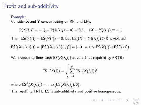
Profit and sub-additivity

Example:Consider X and Y concentrating on RFi and LHj .

P(X (i , j) = −1) = P(X (i , j) = 0) = 0.5, (X + Y )(i , j) ≡ −1.

Then ES(X (i)) = ES(Y (i)) = 0, but ES((X + Y )(i , j)) ≥ 0 is violated,

ES((X+Y )(i)) =∣∣ES((X+Y )(i , j))

∣∣ = |−1| = 1 > ES(X (i))+ES(Y (i)).

We propose to floor each ES(X (i , j)) at zero (not required by FRTB)

ES+(X (i)) =

√√√√ 5∑j=1

ES+(X (i , j))2,

where ES+(X (i , j)) = max{ES(X (i , j)), 0}.

The resulting FRTB ES is sub-additivity and positive homogeneous.

14 / 32

Capital allocation

Consider a portfolio of N risk positions with losses L1, . . . , LN .

The total loss is L =∑N

n=1 Ln.

ρ is a risk measure.

An allocation is a map Law(L1, . . . , LN)→ RN :

Law(L1, . . . , LN) 7→ ρ(Ln | L), for each n,

such thatN∑

ρ(Ln | L) = ρ(L).

Banks need allocations to calculate return on risk-adjusted capital(RORAC):

−E[Ln]

ρ(Ln | L).

RORAC evaluates the capital efficiency of each position.

15 / 32

Capital allocation

Consider a portfolio of N risk positions with losses L1, . . . , LN .

The total loss is L =∑N

n=1 Ln.

ρ is a risk measure.

An allocation is a map Law(L1, . . . , LN)→ RN :

Law(L1, . . . , LN) 7→ ρ(Ln | L), for each n,

such thatN∑

ρ(Ln | L) = ρ(L).

Banks need allocations to calculate return on risk-adjusted capital(RORAC):

−E[Ln]

ρ(Ln | L).

RORAC evaluates the capital efficiency of each position.

15 / 32

Euler allocation principle

Let v1, . . . , vN be a sequence of numbers and Lv =∑N

i=1 vnLn.

Per-unit Euler allocation is

ρ(Ln | L)(v) :=∂

∂vnρ(Lv ).

Setting all vn = 1, we denote the allocation to Ln as ρ(Ln | L).

if ρ is homogeneous of degree 1, Euler’s theorem for homogeneousfunctions implies

ρ(Lv ) =∑n

∂vnρ(Lv ).

Setting v = 1, we have the full allocation property.

16 / 32

Pros and Cons of Euler allocation

Tasche (1999) shows that

(−E[Lv ]

ρ(Lv )

){ > 0, if −E[Li ]ρ(Li | L)(v) >

−E[Lv ]ρ(Lv )

< 0, if −E[Li ]ρ(Li | L)(v) <

−E[Lv ]ρ(Lv )

Denault (2001) uses corporative game (Shapley (1953) andAumann-Shapley (74)) to show that the Euler allocation is the “fair”allocation.

There is no sub-portfolio whose total capital charge is less than the sumof the capital allocations of its components.

However,

I Euler allocation is unstable.

I Euler allocation induces large negative allocations.

17 / 32

Pros and Cons of Euler allocation

Tasche (1999) shows that

(−E[Lv ]

ρ(Lv )

){ > 0, if −E[Li ]ρ(Li | L)(v) >

−E[Lv ]ρ(Lv )

< 0, if −E[Li ]ρ(Li | L)(v) <

−E[Lv ]ρ(Lv )

Denault (2001) uses corporative game (Shapley (1953) andAumann-Shapley (74)) to show that the Euler allocation is the “fair”allocation.

There is no sub-portfolio whose total capital charge is less than the sumof the capital allocations of its components.

However,

I Euler allocation is unstable.

I Euler allocation induces large negative allocations.

17 / 32

Two steps allocation for FRTB

Given liquidity horizon adjusted risk profiles {Xn}1≤n≤N ,

Step 1: allocate to each Xn(i , j)

ρ(Xn(i , j) |X ).

Step 2: allocate to each X̃n(i , k)

ρ(X̃n(i , k) |Xn(i , j)

), k ≥ j .

Then aggregate

ρ(X̃n(i , k) |X ) =k∑

ρ(Xn(i , k)|Xn(i , j)).

18 / 32

ρ(Xn(i, 1)|X) ρ(Xn(i, 5)|X)

ρ(X̃n(i, 1)|X) ρ(X̃n(i, 5)|X)ρ(X̃n(i, 2)|X)

· · ·

Step 1

Step 2

19 / 32

Euler allocation under FRTB

Let v = {v1, . . . , vn} be real numbers

Let X v ,j(i) =∑

n Xvn,jn (i), where

X vn,jn (i) =

(Xn(i , 1), · · · ,Xn(i , j−1), vnXn(i , j),Xn(i , j + 1), · · · ,Xn(i , 5)

For each RFi , we define the Euler allocation for FRTB ES as

ES(Xn(i , j) |X (i)) :=∂

∂vnES(X v ,j(i))

∣∣∣v=1

where v = 1 means all vn = 1.

ES(Xn(i , j) |X (i)) =ES(X (i , j))

ES(X (i))

∂vnES(X v (i , j)

)∣∣∣v=1

where X v (i , j) =∑

n vnXn(i , j).

20 / 32

Euler allocation under FRTB

Let v = {v1, . . . , vn} be real numbers

Let X v ,j(i) =∑

n Xvn,jn (i), where

X vn,jn (i) =

(Xn(i , 1), · · · ,Xn(i , j−1), vnXn(i , j),Xn(i , j + 1), · · · ,Xn(i , 5)

For each RFi , we define the Euler allocation for FRTB ES as

ES(Xn(i , j) |X (i)) :=∂

∂vnES(X v ,j(i))

∣∣∣v=1

where v = 1 means all vn = 1.

ES(Xn(i , j) |X (i)) =ES(X (i , j))

ES(X (i))

∂vnES(X v (i , j)

)∣∣∣v=1

where X v (i , j) =∑

n vnXn(i , j).

20 / 32

I Euler allocation of FRTB ES is a scaled version of the Eulerallocation of regular ES

I Euler allocation of regular ES can be calculated byscenario-extraction (Trashe (1999)):

∂vnES(X v (i , j)

)∣∣∣v=1

= E[Xn(i , j) |X (i , j) ≥ VaR(X (i , j))

I If each X (i , j) is floored at zero, then

ES+(Xn(i , j) |X (i))

{ES+(X (i,j))ES+(X (i)) E

[Xn(i , j) |X (i , j) ≥ VaR(X (i , j))

]if ES(X (i , j)) > 0

0 otherwise.

I Euler allocation of IMCC

IMCCE (Xn(i , j) |X ) := 0.5ESR,S(X (i))

ESR,C(X (i))ESF,C

(Xn(i , j) |X (i)

It is a full allocation.

21 / 32

∂vnES(X v (i , j)

)∣∣∣v=1

= E[Xn(i , j) |X (i , j) ≥ VaR(X (i , j))

ES+(Xn(i , j) |X (i))

[Xn(i , j) |X (i , j) ≥ VaR(X (i , j))

]if ES(X (i , j)) > 0

0 otherwise.

ESR,C(X (i))ESF,C

(Xn(i , j) |X (i)

21 / 32

∂vnES(X v (i , j)

)∣∣∣v=1

= E[Xn(i , j) |X (i , j) ≥ VaR(X (i , j))

ES+(Xn(i , j) |X (i))

[Xn(i , j) |X (i , j) ≥ VaR(X (i , j))

]if ES(X (i , j)) > 0

0 otherwise.

ESR,C(X (i))ESF,C

(Xn(i , j) |X (i)

21 / 32

∂vnES(X v (i , j)

)∣∣∣v=1

= E[Xn(i , j) |X (i , j) ≥ VaR(X (i , j))

ES+(Xn(i , j) |X (i))

[Xn(i , j) |X (i , j) ≥ VaR(X (i , j))

]if ES(X (i , j)) > 0

0 otherwise.

ESR,C(X (i))ESF,C

(Xn(i , j) |X (i)

It is a full allocation.21 / 32

Negative allocations

Hedging among different RFs or LHs does not lead to negativeallocations.

Example:

Consider two loss Y with RFi and Z with RFk , i 6= k ,Y ,Z ∼ N(0, σ), and Y + Z = 0.

Euler of regular ES:

ESR(Y |Y + Z ) + ESR(Z |Y + Z ) = ESR(Y + Z ) = 0.

Then one of two allocations must be negative, say ESR(Y |Y + Z ).

Euler of FRTB ES:Let X be the risk profile containing X and Y . X (i) = Y , X (k) = Z , then

ES(Y |X (i)) = ES(Y ) > 0, ES(Z |X (k)) = ES(Z ) > 0.

Even though Y + Z = 0, IMCC (X ) > 0.

22 / 32

Negative allocations

Hedging among different RFs or LHs does not lead to negativeallocations.

Example:

Consider two loss Y with RFi and Z with RFk , i 6= k ,Y ,Z ∼ N(0, σ), and Y + Z = 0.

Euler of regular ES:

ESR(Y |Y + Z ) + ESR(Z |Y + Z ) = ESR(Y + Z ) = 0.

Then one of two allocations must be negative, say ESR(Y |Y + Z ).

Euler of FRTB ES:Let X be the risk profile containing X and Y . X (i) = Y , X (k) = Z , then

ES(Y |X (i)) = ES(Y ) > 0, ES(Z |X (k)) = ES(Z ) > 0.

Even though Y + Z = 0, IMCC (X ) > 0.

22 / 32

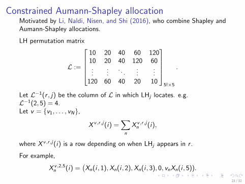
Constrained Aumann-Shapley allocationMotivated by Li, Naldi, Nisen, and Shi (2016), who combine Shapley andAumann-Shapley allocations.

LH permutation matrix

10 20 40 60 12010 20 40 120 60...

.... . .

......

120 60 40 20 10

Let L−1(r , j) be the column of L in which LHj locates. e.g.L−1(2, 5) = 4.

Let v = {v1, . . . , vN},

X v ,r ,j(i) =∑n

X v ,r ,jn (i),

where X v ,r ,j(i) is a row depending on when LHj appears in r .

For example,

X v ,2,5n (i) =

(Xn(i , 1),Xn(i , 2),Xn(i , 3), 0, vnXn(i , 5)).

23 / 32

Constrained Aumann-Shapley allocationMotivated by Li, Naldi, Nisen, and Shi (2016), who combine Shapley andAumann-Shapley allocations.

LH permutation matrix

10 20 40 60 12010 20 40 120 60...

.... . .

......

120 60 40 20 10

Let L−1(r , j) be the column of L in which LHj locates. e.g.L−1(2, 5) = 4.Let v = {v1, . . . , vN},

X v ,r ,j(i) =∑n

X v ,r ,jn (i),

where X v ,r ,j(i) is a row depending on when LHj appears in r .

For example,

X v ,2,5n (i) =

(Xn(i , 1),Xn(i , 2),Xn(i , 3), 0, vnXn(i , 5)).

23 / 32

Constrained Aumann-Shapley allocationWe define the Constrained Aumann-Shapley allocation(CAS) in thepermutation r as

CAS(r ,Xn(i , j)) :=

∂vnES(X v ,r ,j(i))

∣∣∣v=q

CAS(r ,Xn(i , j)) = η(r , i , j)∂

∂vnES(X v (i , j)

)∣∣∣v=1

η(r , i , j) =

√∑1≤s≤L−1(r,j) ES

(X (i ,L(r , s))

)2 −√∑1≤s<L−1(r,j) ES(X (i ,L(r , s))

)2ES(X (i , j)

I CAS is a scaled version of Euler

I Losses with the same LH need to be added to the same portfolio atthe same time, to ensure computational efficiency

24 / 32

Constrained Aumann-Shapley allocationWe define the Constrained Aumann-Shapley allocation(CAS) in thepermutation r as

CAS(r ,Xn(i , j)) :=

∂vnES(X v ,r ,j(i))

∣∣∣v=q

CAS(r ,Xn(i , j)) = η(r , i , j)∂

∂vnES(X v (i , j)

)∣∣∣v=1

η(r , i , j) =

√∑1≤s≤L−1(r,j) ES

(X (i ,L(r , s))

)2 −√∑1≤s<L−1(r,j) ES(X (i ,L(r , s))

)2ES(X (i , j)

I CAS is a scaled version of Euler

I Losses with the same LH need to be added to the same portfolio atthe same time, to ensure computational efficiency

24 / 32

CAS allocation of IMCC

We define the CAS allocation for IMCC as

IMCCC (Xn(i , j) |X ) := 0.5ESR,S(X (i))

ESR,C(X (i))

5!∑r=1

CASF,C(r ,Xn(i , j)).

25 / 32

Stress scaling adjustmentIn the previous two methods, the Xn(i , j) induced risk contribution is not

considered in the stress scaling factor ESR,S(X (i))ESR,C(X (i))

We define the Euler allocation with stress scaling adjustment as

IMCCE,S(Xn(i , j) |X (i)

):= 0.5

[ESR,S(X v ,j(i)

)ESR,C

(X v ,j(i)

)ESF,C(X v ,j(i)

)]∣∣∣v=1

IMCCE,S(Xn(i , j) |X (i)

)= 0.5

[ESR,S(X (i))

ESR,C(X (i))ESF,C

(Xn(i , j) |X (i)

)+ESF,C(X (i))

ESR,C(X (i))ESR,S

(Xn(i , j) |X (i)

)−ESR,S(X (i))ESF,C(X (i))

ESR,C(X (i))2ESR,C

(Xn(i , j) |X (i)

26 / 32

Simulation analysis 1

X̃ (i , j), normal with mean 0 and annual volatility 30%

Risk profiles are simulated for 250 days

Independence among different days

The following correlation structure in the same day:

1. Independence

2. Strong positive correlation among RFs and LHs

3. Strong positive correlation among RFs, independent among LHs

4. Independent among RFs, strong positive correlation among LHs

27 / 32

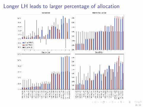
Longer LH leads to larger percentage of allocation

28 / 32

Simulation analysis 2Three hedging structures:

1. Strong hedging between EQ and IR

2. Strong hedging between LH1 and LH2

3. Strong hedging between two risk positions in the same bucket

FRTB allocations produce

I no negative allocations for hedging among different bucket

I some negative allocations for hedging in the same bucket, but withsmaller magnitude

29 / 32

Simulation analysis 2Three hedging structures:

1. Strong hedging between EQ and IR

2. Strong hedging between LH1 and LH2

3. Strong hedging between two risk positions in the same bucket

FRTB allocations produce

I no negative allocations for hedging among different bucket

I some negative allocations for hedging in the same bucket, but withsmaller magnitude

29 / 32

FRTB allocations are more stableHistograms and fitted kernel densities for allocations in Case 3:

30 / 32

Loss in EQ with 40-days LH and CM with 60 days LH have 9 times ofvolatility in the stress period than the normal period.

Two reduced set of risk factors

Set A : Include both RFs with large variations

Set B : Exclude both RFs with large variations

Set A Set A Set B Set B(Adj) (Without adj) (Adj) (Without adj)

CM.60 4.00% 2.24% 1.43% 1.43%EQ.40 5.04% 3.26% 2.11% 2.11%

Table: IMCC(Set A)=11.55 and IMCC(Set B)=3.14

The choice of reduced set of risk factors has large impact on allocations.

31 / 32

Loss in EQ with 40-days LH and CM with 60 days LH have 9 times ofvolatility in the stress period than the normal period.

Two reduced set of risk factors

Set A : Include both RFs with large variations

Set B : Exclude both RFs with large variations

Set A Set A Set B Set B(Adj) (Without adj) (Adj) (Without adj)

CM.60 4.00% 2.24% 1.43% 1.43%EQ.40 5.04% 3.26% 2.11% 2.11%

Table: IMCC(Set A)=11.55 and IMCC(Set B)=3.14

The choice of reduced set of risk factors has large impact on allocations.

31 / 32

Conclusion

Two allocation methods reduce FRTB allocations to Euler allocations

I Computational efficiency

I Easy to adapt to the current system

Simulation analysis shows

I Longer LH leads to more allocation

I Much less negative allocations

I More stable allocations

I Sensitive to the choice of reduced set of risk factors

Thanks for your attention!

32 / 32

Conclusion

Two allocation methods reduce FRTB allocations to Euler allocations

I Computational efficiency

I Easy to adapt to the current system

Simulation analysis shows

I Longer LH leads to more allocation

I Much less negative allocations

I More stable allocations

I Sensitive to the choice of reduced set of risk factors

Thanks for your attention!

32 / 32

capital allocation under fundamental review of trading bookcapital allocation under fundamental...

Documents