capital accumulation and economic growth this chapter we examine the relationship between increases...

Capital Accumulation and Economic Growth

Overview

In this chapter we examine the relationship between increases in the capital stock and economic growth. We first

discuss whether an economy can always grow if it increases only its capital stock. Under certain plausible assump-

tions, we show this is not possible, and that poorer countries should therefore grow faster than wealthy ones,

whose economies will depend more on technological progress than capital accumulation. We then discuss why

countries with high investment rates also have high standards of living. We show that to have a high standard of

living a country must, over the long run, have a high level of savings and investment. We then examine why some

countries have such low savings rates and whether governments can alter this. Finally we consider the rapid

growth of the Southeast Asian economies and the extent to which they have relied on capital accumulation.

5.1 Introduction: What Is the Capital Stock?

THE LINK BETWEEN CAPITAL AND OUTPUT

As we outlined at the end of Chapter 4, increases in the capital stock are a major fac-tor in explaining growth in industrialized countries over the last 100 years and in ac-counting for differences in the standard of living among countries. Figure 5.1a plots

84

C H A P T E R 5

per capita real gross domestic product (GDP) and the per capita capital stock for agroup of industrialized and developing countries. Figure 5.1b focuses on the growthin GDP and the growth in the capital stock between 1965 and 1990 for the samegroup of countries. Countries that have had large increases in their capital stockhave also seen large increases in their GDP. For instance, Botswana during this pe-riod has seen a near 20-fold increase in its capital stock, and largely as a conse-quence, its GDP per capita has more than quadrupled. This represents both thelargest increase in capital and the largest increase in GDP per capita of all of thesecountries. Similarly Japan had both the second highest proportional increase in itscapital stock and the second highest percentage increase in GDP. Evidently capitalaccumulation matters greatly for both a country’s standard of living and its rate ofgrowth.

5.1 Introduction: What Is the Capital Stock? 85

00

2000

4000

6000

8000

10,000

12,000

14,000

16,000

18,000

20,000

10,000 20,000

Capital stock per worker 1990

30,000 40,000 50,000

India

Botswana

Nigeria Mexico

Israel Spain

Italy

AustraliaDenmark

Japan

Canada

SwedenR

eal G

DP

per

cap

ita (

1985

$)

F I G U R E 5 . 1 a GDP per capita versus capital stock per worker in 1990. Source: Summers and Hestondataset, Penn World Tables 5.5, http:/www.nber.org

0 5 10 15 20 25

Ratio of 1990 to 1965 value

Israel

Italy

Denmark

India

Canada

Botswana

GDP

Capital

F I G U R E 5 . 1 b Capitalgrowth and GDP growth 1965–90.Countries that haveaccumulated substantialstocks of productive capitalhave reached higherstandards of living. Source:Summers and Heston, PennWorld Table 5.5,http:/www.nber.org

WHAT IS CAPITAL?

Before considering how capital accumulation boosts output, we have to be more preciseabout what we mean by capital. Broadly speaking, there are two categories of capital:machines and buildings (sometimes also called equipment and structures, respectively).Production requires both types of capital—car firms could not operate without a sitethat protected machines and workers from the elements, and even service sector firmsneed machinery (telephones, computers, etc.) to produce their output.

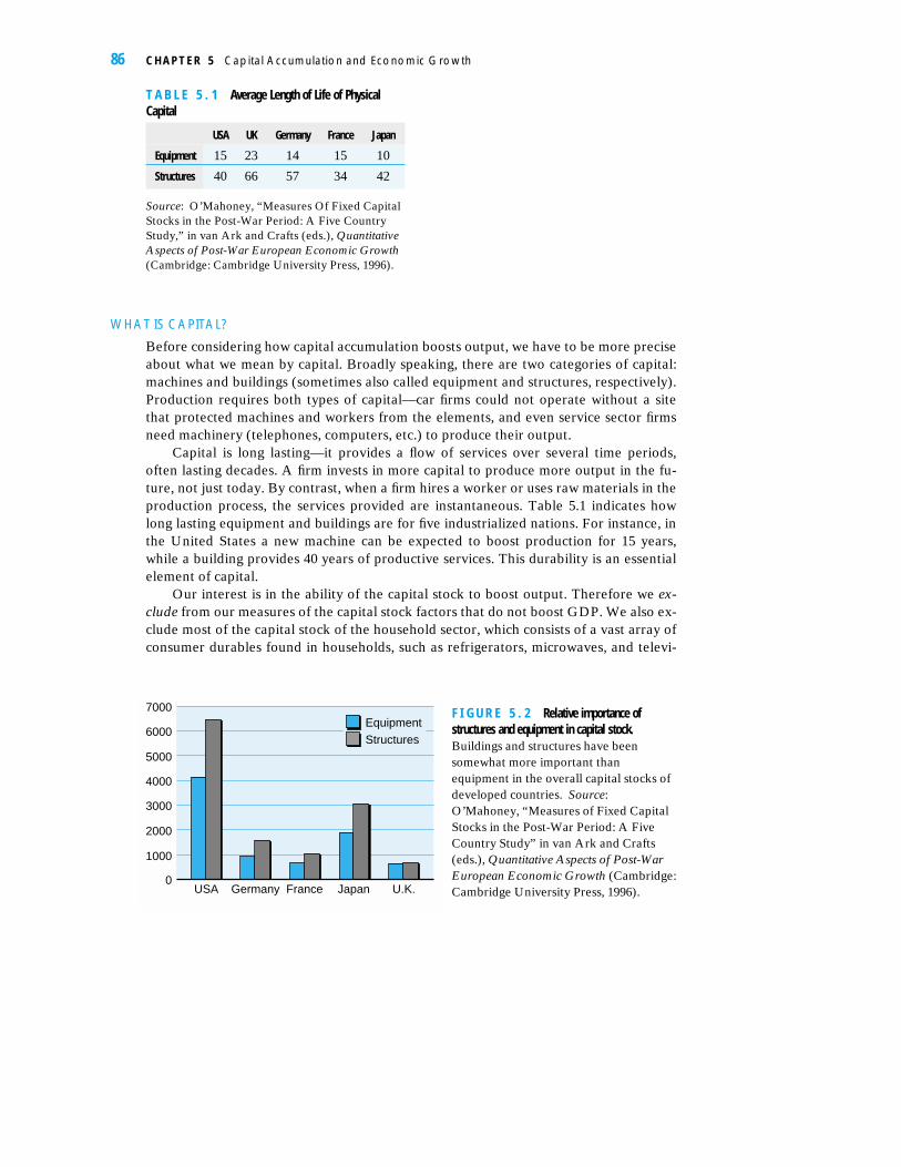
Capital is long lasting—it provides a flow of services over several time periods,often lasting decades. A firm invests in more capital to produce more output in the fu-ture, not just today. By contrast, when a firm hires a worker or uses raw materials in theproduction process, the services provided are instantaneous. Table 5.1 indicates howlong lasting equipment and buildings are for five industrialized nations. For instance, inthe United States a new machine can be expected to boost production for 15 years,while a building provides 40 years of productive services. This durability is an essentialelement of capital.

Our interest is in the ability of the capital stock to boost output. Therefore we ex-clude from our measures of the capital stock factors that do not boost GDP. We also ex-clude most of the capital stock of the household sector, which consists of a vast array ofconsumer durables found in households, such as refrigerators, microwaves, and televi-

86 C H A P T E R 5 Capital Accumulation and Economic Growth

T A B L E 5 . 1 Average Length of Life of PhysicalCapital

USA UK Germany France Japan

Equipment 15 23 14 15 10

Structures 40 66 57 34 42

Source: O’Mahoney, “Measures Of Fixed CapitalStocks in the Post-War Period: A Five CountryStudy,” in van Ark and Crafts (eds.), QuantitativeAspects of Post-War European Economic Growth(Cambridge: Cambridge University Press, 1996).

EquipmentStructures

0

1000

2000

3000

4000

5000

6000

7000

USA Germany France Japan U.K.

F I G U R E 5 . 2 Relative importance ofstructures and equipment in capital stock.Buildings and structures have beensomewhat more important thanequipment in the overall capital stocks ofdeveloped countries. Source:O’Mahoney, “Measures of Fixed CapitalStocks in the Post-War Period: A FiveCountry Study” in van Ark and Crafts(eds.), Quantitative Aspects of Post-WarEuropean Economic Growth (Cambridge:Cambridge University Press, 1996).

sions. These commodities should last (hopefully!) for years and provide a flow of ser-vices, but these services are not recorded in GDP.1

We should therefore think of our measure of the capital stock as the machines andbuildings used in the production of GDP. This raises the issue of which form of capi-tal—machines or buildings—is more important. Figure 5.2 shows that for industrializednations buildings account for around 60% of the capital stock. Figure 5.3 illustrates (forthe United States) that the trend in both forms of capital is the same. Economic growthcomes about through increases in both equipment and structures.

HOW LARGE IS THE CAPITAL STOCK?

The other important fact to note about the capital stock is its size relative to the economy.Table 5.2 shows the ratio of the capital stock to GDP for a range of industrial countries.The capital stock is generally between two and three times the size of GDP (it would bemuch larger if we included the residential housing stock). We would expect this given the

5.1 Introduction: What Is the Capital Stock? 87

1GDP does include the rental services of residential property. However, our focus is on the produc-tion process, so unless we state otherwise, our capital stock measures will also exclude the residentialhousing stock.

1952 1956 1960 1964 1968 1972 1976 1980 1984 1988

Structures

Equipment

0

2000

4000

6000

8000

10,000

12,000

1985

$bn

F I G U R E 5 . 3 U.S. capital stock 1948–89. In the period since the Second World War, U.S. stocks ofequipment and of buildings and other structures have grown broadly in line. Source: O’Mahoney.“Measures Of Fixed Capital Stocks In The Post-War Period: A Five Country Study,” in van Arkand Crafts (eds.), Quantative Aspects of Post-War European Economic Growth (Cambridge:Cambridge University Press, 1996).

T A B L E 5 . 2 Capital Stock Divided by GDP, 1992

USA France Germany Netherlands UK Japan

Machinery and Equipment 0.86 0.74 0.70 0.78 0.65 1.07

Nonresidential Structures 1.57 1.52 1.63 1.53 1.17 1.95

Total 2.43 2.26 2.33 2.31 1.82 3.02Source: Table 2.1 Maddison, Monitoring the World Economy: 1820–1992(Paris: OECD, 1995).

durability of capital. Annual GDP measures the flow of output produced from the stock ofcapital over a given year. But capital is long lasting so that the flow (GDP) is small relativeto the stock (capital), and hence the capital–output ratio is substantially greater than 1.

5.2 Capital Accumulation and Output Growth

HOW MUCH EXTRA OUTPUT DOES A NEW MACHINE PRODUCE?

We now discuss how increases in the capital stock lead to increases in output, our firststep in constructing a model of economic growth. First we consider a purely technologi-cal question about the production function, namely, what happens to output when acountry increases its capital stock? The answer will strongly affect how we view theprocess of economic growth.

As we discussed in Chapter 4, this technological question is about the marginalproduct of capital—how does output increase when a country increases its capitalstock? Remember that the marginal product of capital is about what happens to outputwhen only the capital stock changes: in other words, when a country invests in capitalbut leaves unchanged the amount of labor employed and the technology in use. Notethat we are not taking any account of whether there will be demand for the additionaloutput created—our sole concern is the technological relationship between increasedcapital input and increased output.

The key question is how the marginal product of capital varies. In particular, howdoes the extra output that another unit of capital produces compare with the output thatthe last unit of capital installed produced? Consider the case of a firm that publishes text-books and has four printing presses. The introduction of the fourth printing press enabledthe firm to increase its production by 500 books per week. Will a fifth machine increaseproduction by more than 500 books, by less than 500 books, or just 500 more books? Ifthe fifth machine leads to an increase in production of more than 500 books (the increasethe fourth machine generated), then we have an increasing marginal product of capital. Ifthe increased production is less than 500 books, then we have a decreasing marginalproduct, and if the increase equals 500, then we have a constant marginal product.

Answering this question is about technology, not economics. It is a question aboutwhat the world is actually like, and we can answer by observing what happens in partic-ular firms or industries. Marginal product may be increasing in some industries and de-creasing in others. Over some range of capital, an industry may face an increasingmarginal product, but beyond a certain stage of development, the marginal productmay begin to fall.

DECREASING MARGINAL PRODUCT, OR IT DOESN’T GET ANY EASIER

In this chapter we shall assume that the marginal product of capital is decreasing for theaggregate economy and discuss what this implies for economic growth. In Chapter 7 weconsider alternative assumptions and the empirical evidence for them.


Why might the marginal product of capital be decreasing? Consider again the pub-lishing company and assume that it has 10 employees, each working a fixed shift. Withfour machines, there are already two and a half employees per machine. But as we in-crease the number of machines but hold fixed the technology and hours worked, we aregoing to encounter problems. There will be fewer and fewer operator hours to monitorthe machines, so each machine will probably be less productive. Even if each new ma-chine produces extra output, that the boost in output will probably not be as high asfrom the previous machine. Note the importance of assuming that labor input and tech-nology remain unchanged.

Obviously not all technologies will be characterized by decreasing marginal prod-uct. Consider the case of a telephone. When a country has only one telephone, the mar-ginal product of that investment is zero—there is no one to telephone! Investment in asecond telephone has a positive boost to output; there is now one channel of communi-cation. Investment in a third telephone substantially increases communications—thereare now three communication links, and so the investment increases the marginal prod-uct of capital. Adding more and more telephones increases even further the number ofpotential communication links.2 Telephones are an example of a technology that bene-fits from network effects, as is the case with information technology generally (seeChapter 6). Network effects operate when the benefits of being part of a network in-crease with the number of people using the network. Therefore not all technologieshave to have decreasing marginal product.

Figure 5.4 shows the case of diminishing marginal product of capital. At point Athe country has little capital, so new investment leads to a big boost in output. At pointB the capital stock is so large that each new machine generates little extra output. Notethat we have assumed that new machines always increase output—albeit by smallamounts—when the capital stock is high.

Figure 5.4a shows how the capital stock is related to increases in output (the mar-ginal product of capital), but we can also use this relationship to draw a productionfunction summarizing how the stock of capital is linked to the level of output. This isshown in Figure 5.4b. At low levels of capital, the marginal product is high, so that smallincreases in the capital stock lead to a big jump in output, and the production functionis steeply sloped. Thus point A in Figure 5.4b corresponds to the same point in Figure

5.2 Capital Accumulation and Output Growth 89

2If the number of telephone lines is n, then addition of a new line creates n new potential connections.

A B

Capital stock

Mar

gtin

al p

rodu

ctof

cap

ital

F I G U R E 5 . 4 a Marginal product of capital.

5.4a. However, at high levels of capital (such as point B), each new machine generatesonly a small increase in output, so that the production function starts to flatten out—output changes little in this range even for large changes in the capital stock. Figure5.4b will feature prominently in the rest of this chapter as we discuss how much a coun-try can grow through capital accumulation.

5.3 Capital Stock and Interest Rates

CHOOSING THE CAPITAL STOCK

The marginal product of capital is crucial for determining how much capital a firm or acountry should accumulate.3 The extra revenue a new machine contributes is the priceat which output is sold (p) multiplied by the marginal product of capital (MPK). If thisamount is greater than the cost of a new machine (which we shall denote r) then it isprofitable for a firm to install the machinery. So if MPK� r/p it is profitable to add tothe capital stock. Therefore in Figure 5.5 at A, the marginal product of capital is higher


3Note once again that what we mean by investment here are increases in the capital stock ratherthan the more common usage in newspapers where investment refers to the purchase of financial assets.

A B

Capital stock

Out

put

F I G U R E 5 . 4 b The production function. A concaveproduction function implies a declining marginalproduct of capital.

A

B

C

Capital stock

Cos

t of c

apita

l

Increased costof capital r1/p

Cost ofcapital r0/p

Marginal productof capital

CA

CB

CCF I G U R E 5 . 5 Investmentand the cost of capital. Increasesin the cost of capital reducethe optimal capital stock.

than the cost of an additional machine (given by the horizontal line r0/p), so the firm in-creases its capital stock until it reaches B, where the last machine contributes just asmuch to revenues as it does to cost. By contrast, at C each new machine loses money, sothe capital stock should be reduced.

This discussion raises the issue of what determines the cost of capital. For the mo-ment we shall consider just one element: the interest rate.4 We can think of the cost ofthe machine as the interest rate (r) that would need to be paid on a loan used to buy it.If we assume that it costs 1 to buy a unit of capital (so we measure everything in termsof the price of a machine) then the interest cost is just r. An alternative way of seeingthe point is to note that rather than purchase a new machine, a firm could invest thefunds in a bank account and earn interest. Therefore to be profitable, the investmentproject must produce at least the rate of interest. If the marginal product of capital isabove the interest rate, then firms will continue to invest in more machines until, be-cause of decreasing marginal product, there is no additional advantage from doing so—the marginal product equals the interest rate. As the interest rate changes, so does thedesired level of capital—if the interest rate increases, then the cost of capital shifts tor1/p (as in Figure 5.6) and the firm desires less capital, while if the interest rate falls, in-vestment demands will be high. Therefore the relationship between investment and theinterest rate is negative, as shown in Figure 5.6.

DETERMINING INTEREST RATES

However, while a firm may wish to increase its capital stock, given the level of interestrates, it has to finance this increase. Either the firm has to use its own savings or borrowthose of other economic agents. We assume that as interest rates increase, so does thelevel of savings. In other words, as banks or financial markets offer higher rates of re-turn on savings, individuals and firms respond by spending less and saving more. There-fore the relationship between savings and the interest rate is positive. Figure 5.6 showsthis relationships among savings, investment, and the interest rate.

5.3 Capital Stock and Interest Rates 91

4Chapter 14 considers in far more detail the investment decision and shows that the cost of capitalmust also include allowance for depreciation, changes in the price of capital goods, and taxes.

RA

SA IA IB

RB

RC

Output

Investment schedule shifts out because of technological progress

Savings(increasingwith interestrates)

F I G U R E 5 . 6 Investment, savings, and interestrates. Technical progress increasesinvestment and may also drive rates ofreturn (interest rates) up.

Consider the case where the interest rate is RA. At this level interest rates are solow that savers are not prepared to save much, and savings are at SA. However, low in-terest rates make capital investment attractive as the marginal product of capital ishigher than the interest rate. As a result, firms are keen to borrow and desire invest-ment IA. There are not enough savings to finance this desired level of investment, whichfrustrates some firms’ investment plans. Because of the gap between the marginal prod-uct of capital and the interest rate, firms are prepared to pay a higher interest rate toraise funds for investment. This puts upward pressure on interest rates, which in turnleads to increases in savings, which can be used to finance the desired investment. Thisadditional savings will in turn help alleviate the imbalance between savings and invest-ment. This process will continue—with interest rates increasing—until savings equal in-vestment at the interest rate RB. At this point firms will not be demanding more loanfinance because the interest rate is such that additional investment is not profitable. Atthis point the cost of capital just matches the value of the extra output produced; withdecreasing MPK any extra investment will generate a lower value of extra output thanthe extra cost involved.

5.4 Why Poor Countries Catch Up with the Rich

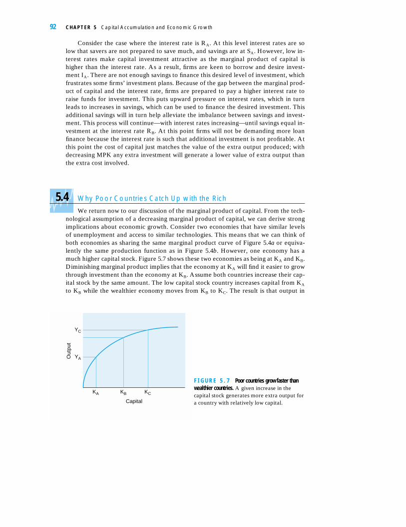
We return now to our discussion of the marginal product of capital. From the tech-nological assumption of a decreasing marginal product of capital, we can derive strongimplications about economic growth. Consider two economies that have similar levelsof unemployment and access to similar technologies. This means that we can think ofboth economies as sharing the same marginal product curve of Figure 5.4a or equiva-lently the same production function as in Figure 5.4b. However, one economy has amuch higher capital stock. Figure 5.7 shows these two economies as being at KA and KB.Diminishing marginal product implies that the economy at KA will find it easier to growthrough investment than the economy at KB. Assume both countries increase their cap-ital stock by the same amount. The low capital stock country increases capital from KA

to KB while the wealthier economy moves from KB to KC. The result is that output in


F I G U R E 5 . 7 Poor countries grow faster thanwealthier countries. A given increase in thecapital stock generates more extra output fora country with relatively low capital.

YC

YA

KA KB KC

Capital

Out

put

the low capital country rises from YA to YB and in the richer economy from YB to YC.Therefore, the same investment will bring forth a bigger increase in output in thepoorer economy than the richer one. In other words, because of decreasing marginalproduct, growth from capital accumulation becomes more and more difficult the higherthe capital stock of a country becomes. This “catch-up” result implies a process of con-vergence among countries and regions—for the same investment poorer countries willgrow faster than wealthier ones, so wealth inequalities across countries should decreaseover time.

Figure 5.8, which displays the dispersion (as measured by the standard deviation)of income per head across U.S. states, shows some evidence for this. Since 1900 the in-equalities of income across states have been dramatically reduced as poorer states, suchas Maine and Arkansas, have grown faster than wealthier ones, such as Massachusettsand New York. This is entirely consistent with the assumption of decreasing marginalproduct and its implication of catch up.

Comparing income across U.S. states is a good test of the theoretical predictions ofcatch-up because our analysis depends on countries or regions sharing the same pro-duction function (i.e., similar unemployment rates and access to similar technology).This is likely to be the case comparing across U.S. states. But finding other examples ofcountries that satisfy these conditions is not easy—low capital countries like India orBotswana also tend to have access to lower levels of technology than countries such asJapan or Australia. However, the circumstances of war and subsequent economic re-covery offer some further support for assuming decreasing marginal product. Figure 5.9shows that between 1945 and 1946, just after World War II, West German capital stockand output both fell. However, between 1947 and 1952, the German economy grew farmore rapidly than over the previous decade. It achieved this rapid growth with onlysmall increases in the capital stock—the ratio of output growth to capital growth duringthis period was extremely high. In other words, small levels of investment producedhigh levels of output growth compared to the years before 1945—exactly what decreas-ing marginal product would predict. The large drop in the capital stock between 1944and 1947, the result of Germany’s losing the war, meant that investment in 1947 wouldbenefit from a much higher marginal product of capital compared to 1943. Table 5.3shows a similarly sharp bounce back in output after WWII for other European nations.

5.7 Why Poor Countries Catch Up with the Rich 93

18900

0.1

0.2

0.3

0.4

0.5

0.6

1910 1930 1950 1970 1990

Inco

me

disp

ersi

on Without transfers

With transfers (since 1929)

F I G U R E 5 . 8 Income dispersionacross U.S. states. Income inequalitybetween states in the Untied Stateshas declined greatly since the end ofthe nineteenth century. Source:Baro and Sala-I-Martin, EconomicGrowth (New York: McGraw Hill,1995). (Transfers are governmenttransfers of income.)

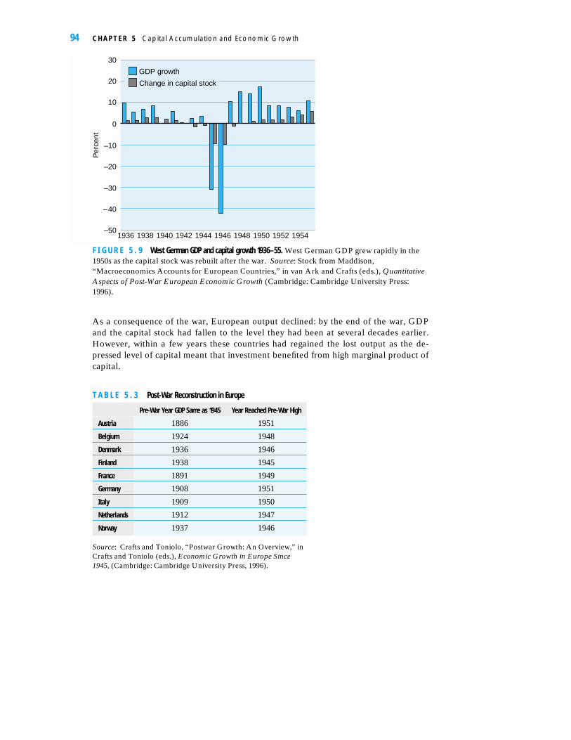
As a consequence of the war, European output declined: by the end of the war, GDPand the capital stock had fallen to the level they had been at several decades earlier.However, within a few years these countries had regained the lost output as the de-pressed level of capital meant that investment benefited from high marginal product ofcapital.


–50

–40

–30

–20

–10

0

10

20

30

1936 1938 1940 1942 1944 1946 1948 1950 1952 1954

Per

cent

GDP growth

Change in capital stock

F I G U R E 5 . 9 West German GDP and capital growth 1936–55. West German GDP grew rapidly in the1950s as the capital stock was rebuilt after the war. Source: Stock from Maddison,“Macroeconomics Accounts for European Countries,” in van Ark and Crafts (eds.), QuantitativeAspects of Post-War European Economic Growth (Cambridge: Cambridge University Press:1996).

T A B L E 5 . 3 Post-War Reconstruction in Europe

Pre-War Year GDP Same as 1945 Year Reached Pre-War High

Austria 1886 1951

Belgium 1924 1948

Denmark 1936 1946

Finland 1938 1945

France 1891 1949

Germany 1908 1951

Italy 1909 1950

Netherlands 1912 1947

Norway 1937 1946

Source: Crafts and Toniolo, “Postwar Growth: An Overview,” inCrafts and Toniolo (eds.), Economic Growth in Europe Since1945, (Cambridge: Cambridge University Press, 1996).

5.5 Growing Importance of Total Factor Productivity

The previous section showed that due to diminishing marginal product of capital,wealthier countries find it hard to maintain fast growth through capital accumulationalone. In this section we show a further implication of diminishing marginal product—total factor productivity (TFP) is more important for wealthier economies than poorerones.

To see the intuition behind this result, imagine two publishing firms each with 10employees. One firm has three printing presses, while the other has ten. Consider theimpact one more machine will have for each firm compared to the introduction of newsoftware that improves the productivity of all machines. For the firm with only threemachines, the technological progress (the new software) will have only a limited ef-fect—with only three machines, the software will not improve productivity a lot. How-ever, this firm gains significantly from the introduction of a new machine because itscapital stock is so low that its marginal product of capital is high. By contrast, the otherfirm already has as many machines as employees, so it will benefit very little from an ad-ditional printing press. However, with ten machines to operate, the technologicalprogress will have a more substantial impact. Therefore we can expect capital accumu-lation to be more important for growth relative to TFP for poorer nations, whereas forcapital rich countries we expect the opposite. This is exactly what we saw in Figure 4.12in Chapter 4 for the more mature industrialized nations and emerging markets.

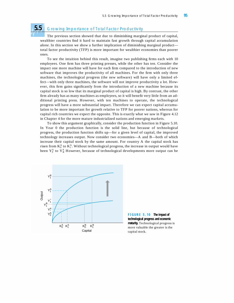
To show this argument graphically, consider the production function in Figure 5.10.In Year 0 the production function is the solid line, but because of technologicalprogress, the production function shifts up—for a given level of capital, the improvedtechnology increases output. Now consider two economies—A and B—both of whichincrease their capital stock by the same amount. For country A the capital stock hasrisen from to . Without technological progress, the increase in output would havebeen to However, because of technological developments more output can beYA

*YA0

KA1KA

0

5.5 Growing Importance of Total Factor Productivity 95

Y1A

K0A K1

A K0

Out

put

Capital

B BK1

Y1*

Y1B

Y*A

Y0A

Y1B

F I G U R E 5 . 1 0 The impact oftechnological progress and economicmaturity. Technological progress ismore valuable the greater is thecapital stock.

produced for any given level of capital, so that with a capital stock country A canproduce in Year 1.

In Figure 5.10 we see that output has increased by a total of � , of which (� ) is due to the addition of extra capital and ( � ) to technological progress.We can use the same argument for country B and show that capital accumulation (with-out technological progress) leads to an increase in output of ( � ), whereas at thisnew higher level of capital ( ), the improved technology increases output ( � ).As the diagram shows, the proportion of growth that TFP explains is higher in countryB than country A—technological progress has a bigger impact for capital rich countries.This implies that wealthier economies, such as those belonging to the OECD, will havea much greater dependence on TFP for producing economic growth than less devel-oped nations. By contrast, emerging economies will be more reliant on capital accumu-lation than they will on TFP, a conjecture that Figure 5.11 supports. For the periodsconsidered in the figures, we suggest that the OECD countries were high capital stockcountries, the Asian economies low capital stock countries, and Latin Americaneconomies in the middle. Clearly TFP has been much more important for growthamong the more developed nations.

5.6 The End of Growth through Capital Accumulation

THE STEADY STATE—A POINT OF REST

We have just shown how the relative importance of capital accumulation declines as thecapital stock increases. In this section we go further and show how countries alwaysreach a point where they cannot grow any more from capital accumulation alone. Cru-cial to this section is the notion of a “steady state”:

D E F I N I T I O N

A steady state is a point where capital accumulation alone will not increase output any further.

YB*YB

1KB1

YB0YB

*

YA*YA

1YA0

YA*YA

0YA1

YA1

KA1


0 20 40 60

East Asia1966–90

Latin America1940–80

OECD1947–73

Proportion of growth due to TFP

F I G U R E 5 . 1 1 Importance of TFP in growth.Source: Crafts, “Productivity GrowthReconsidered” Economic Policy (1992) vol.15, pp. 388–426.

As this definition makes clear the steady state is the point at which the economyceases to grow because of capital accumulations alone.5 The steady state is a point ofrest for the capital stock—efforts to raise or lower the capital stock are futile, and it willalways return to this equilibrium level. Why is this so?

INVESTMENT AND DEPRECIATION

Two factors cause the capital stock to change over time. The first is that firms invest innew machinery and structures, so that the capital stock is increasing. But another factor,“depreciation,” reduces the capital stock. Whenever they are used machines are subjectto wear and tear and breakdown. This means that over time machines become less ef-fective in production unless they are repaired or maintained. Economists call thisprocess of deterioration depreciation—the reduction over time in the productive capa-bilities of capital. Note that economists use the term “depreciation” in a different sensethan accountants do. In accounting, “depreciation” refers to the writing down of thebook value of an asset, which may bear little relation to the physical ability of a ma-chine to produce output.

Because of depreciation, we need to distinguish between different measures of in-vestment. In Chapter 2 we discussed investment as a part of the national accounts of acountry. This is often called gross fixed capital formation, where gross means that no al-lowance is made for the loss of capital through depreciation. Gross investment is theamount of new capital being added to an economy and includes both the repair and re-placement of the existing capital stock as well as new additions to it. Net investment isequal to gross investment less depreciation and represents the increase in the net capi-tal stock—in other words, it deducts repairs and replacements from the new capitalstock being added to an economy. Net investment is therefore equivalent to the in-crease in the capital stock from one year to another. Figure 5.12 shows, for a sample ofdeveloped economies, gross investment and depreciation as a percentage of GDP andsuggests that net investment is about 5–10% of GDP.

5.6 The End of Growth through Capital Accumulation 97

5Although, as we shall see in Chapter 6, technological progress will provide incentives for furthercapital accumulation. This section shows that without technological progress the capital stock does notchange.

Italy France Germany

Investment and Depreciation 1996

U.K. U.S.

Depreciation/GDPGross fixed capitalformation/GDP

0

5

10

15

20

25

Per

cent

F I G U R E 5 . 1 2 Investment and depreciationin selected OECD countries. Gross investmentis substantially higher than net investmentfor developed countries because theirstocks of capital are high. Source: OECDMain Economic Indicators.

Allowing for gross investment and depreciation, the capital stock evolves over timeas

K(t) � K(t � 1) � I(t) � D(t)

where K(t) is the capital stock at time t, I(t) is gross investment, and D(t) is deprecia-tion: I(t) � D(t) is net investment. The steady state is the point where the capital stockdoes not change, so that K(t) � K(t � 1), which can only occur when I(t) � D(t) orwhere gross investment equals depreciation. The country purchases just enough ma-chinery each period to make good depreciation.

CONVERGENCE

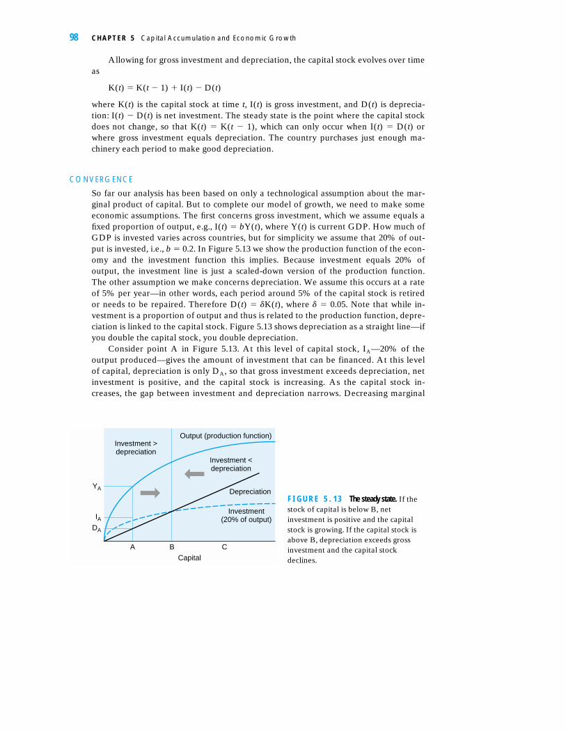
So far our analysis has been based on only a technological assumption about the mar-ginal product of capital. But to complete our model of growth, we need to make someeconomic assumptions. The first concerns gross investment, which we assume equals afixed proportion of output, e.g., I(t) � bY(t), where Y(t) is current GDP. How much ofGDP is invested varies across countries, but for simplicity we assume that 20% of out-put is invested, i.e., b � 0.2. In Figure 5.13 we show the production function of the econ-omy and the investment function this implies. Because investment equals 20% ofoutput, the investment line is just a scaled-down version of the production function.The other assumption we make concerns depreciation. We assume this occurs at a rateof 5% per year—in other words, each period around 5% of the capital stock is retiredor needs to be repaired. Therefore D(t) � �K(t), where � � 0.05. Note that while in-vestment is a proportion of output and thus is related to the production function, depre-ciation is linked to the capital stock. Figure 5.13 shows depreciation as a straight line—ifyou double the capital stock, you double depreciation.

Consider point A in Figure 5.13. At this level of capital stock, IA—20% of theoutput produced—gives the amount of investment that can be financed. At this levelof capital, depreciation is only DA, so that gross investment exceeds depreciation, netinvestment is positive, and the capital stock is increasing. As the capital stock in-creases, the gap between investment and depreciation narrows. Decreasing marginal


A B C

YA

IADA

Capital

Investment >depreciation

Investment <depreciation

Depreciation

Investment(20% of output)

Output (production function)

F I G U R E 5 . 1 3 The steady state. If thestock of capital is below B, netinvestment is positive and the capitalstock is growing. If the capital stock isabove B, depreciation exceeds grossinvestment and the capital stockdeclines.

product implies that each new machine leads to a smaller boost in output than theprevious one. Because investment is a constant proportion of output, this means eachnew machine produces ever smaller amounts of new investment. However, deprecia-tion is at a constant rate—each new machine adds 5% of its own value to the depreci-ation bill. Therefore the gap between investment and depreciation narrows. At pointB the depreciation and investment lines intersect. This defines the steady state capitalstock where gross investment equals depreciation. At this point the last machine addsjust enough extra output to provide enough investment to make good the extra depre-ciation it brings. At this point the capital stock is neither rising nor falling but staysconstant.

Imagine instead that the economy starts with a capital stock of C. At this point de-preciation is above investment, net investment is negative, and the capital stock is de-clining. The country has so much capital that the marginal product of capital is low. Asa consequence, each machine cannot produce enough output to provide the invest-ment to cover its own depreciation, and so the capital stock moves back to the steadystate at B.

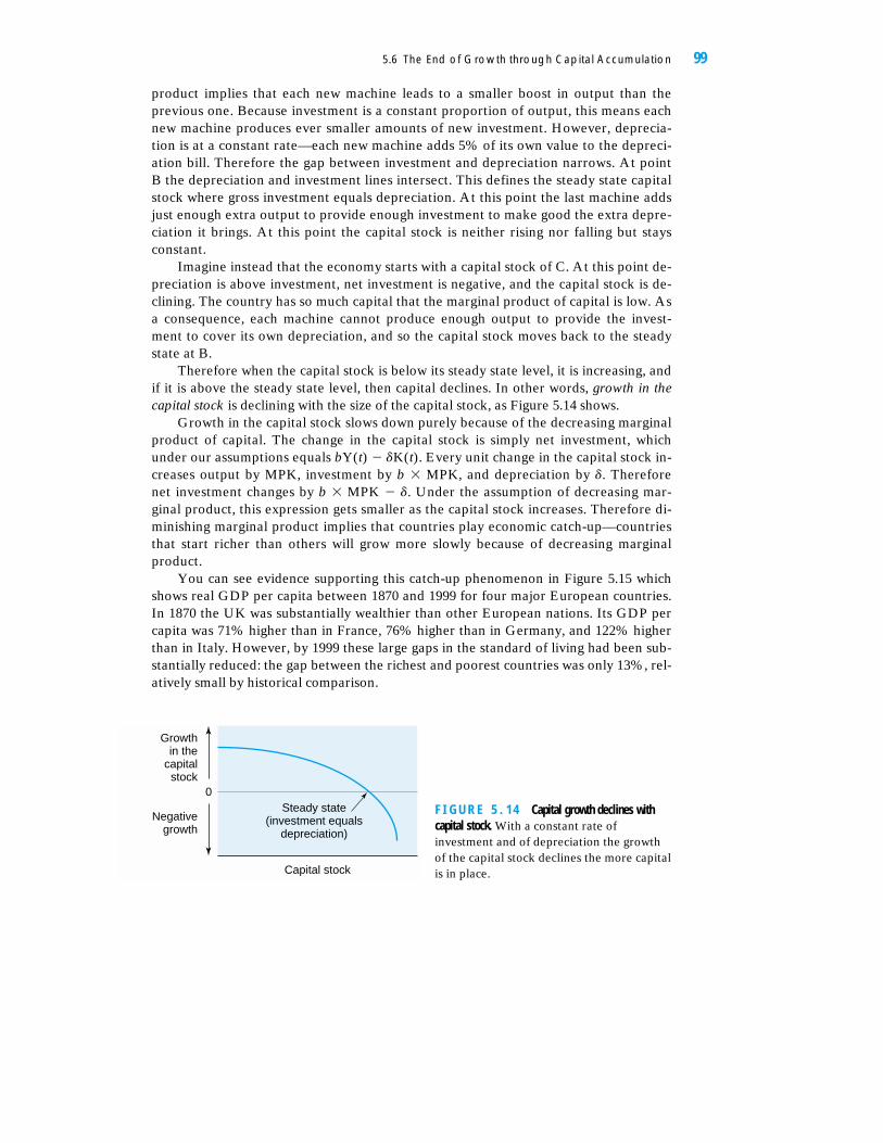
Therefore when the capital stock is below its steady state level, it is increasing, andif it is above the steady state level, then capital declines. In other words, growth in thecapital stock is declining with the size of the capital stock, as Figure 5.14 shows.

Growth in the capital stock slows down purely because of the decreasing marginalproduct of capital. The change in the capital stock is simply net investment, whichunder our assumptions equals bY(t) � �K(t). Every unit change in the capital stock in-creases output by MPK, investment by b � MPK, and depreciation by �. Thereforenet investment changes by b � MPK � �. Under the assumption of decreasing mar-ginal product, this expression gets smaller as the capital stock increases. Therefore di-minishing marginal product implies that countries play economic catch-up—countriesthat start richer than others will grow more slowly because of decreasing marginalproduct.

You can see evidence supporting this catch-up phenomenon in Figure 5.15 whichshows real GDP per capita between 1870 and 1999 for four major European countries.In 1870 the UK was substantially wealthier than other European nations. Its GDP percapita was 71% higher than in France, 76% higher than in Germany, and 122% higherthan in Italy. However, by 1999 these large gaps in the standard of living had been sub-stantially reduced: the gap between the richest and poorest countries was only 13%, rel-atively small by historical comparison.

5.6 The End of Growth through Capital Accumulation 99

Capital stock

0

Growthin the

capitalstock

Negativegrowth

Steady state(investment equals

depreciation)

F I G U R E 5 . 1 4 Capital growth declines withcapital stock. With a constant rate ofinvestment and of depreciation the growthof the capital stock declines the more capitalis in place.

5.7 Why Bother Saving?

INVESTMENT AND THE STANDARD OF LIVING

Because the steady state is the point at which there is no growth through capital accu-mulation, growth at the steady state must be due either to increases in labor input or toimprovements in TFP. Assuming that countries cannot continually reduce their unem-ployment rate, and that all countries eventually have access to the same technology, thisimplies that at the steady state countries will all grow at the same rate. In particularwhether one country is investing more than another does not matter—at the steadystate, capital accumulation does not influence the growth rate. Why then should countriesencourage high levels of investment if such investment makes no difference to the longrun growth rate?

The answer to this question is simple. While the amount of investment makes nodifference to the growth of the economy, it strongly influences the level of capital insteady state. In other words, while the growth of output in the steady state does not de-pend on investment, the level of output does. The more investment a country does, thehigher its steady state standard of living.

To see this, imagine two countries, one of which invests 20% of its output and theother which invests 30%, as in Figure 5.16. Otherwise both countries are identical—theyhave access to the same production function, have the same population and the same de-preciation rate. For both countries their steady state occurs at the point at which invest-ment equals depreciation—KL for the low investment rate country and KH for the highinvestment country. Therefore the level of output in the low investment country is YL,substantially below YH. Countries with low investment rates will therefore have a lowerstandard of living (measured by GDP per capita) than countries with high investmentrates. Low investment rates can only fund a low level of maintenance, so the steady stateoccurs at a low capital stock and, via the production function, at a low output level.

However, at the steady state, both countries will be growing at the same rate—the rateat which technological improvements lead to improvements in the production function.

Therefore, while long-term growth rates are independent of the investment rate,the level of GDP per capita is definitely related to the amount of investment. High in-vestment countries are wealthier than low investment countries, as Figure 5.17 shows.


France

Germany

Italy

U.K.

1870 1929 1950 19767.0

7.5

8.0

8.5

9.0

9.5

10.0

10.5

Loga

rithm

ic s

cale F I G U R E 5 . 1 5 Convergence in GDP per

capita in Europe. Levels of output in themajor four European industrialcountries have converged since the endof the nineteenth century. Source:Maddison, Monitoring the WorldEconomy, 1820–1992 (Paris: OECD,1995). Updated to 1999 from 1994 byauthor using IMF data.

5.7 Why Bother Saving? 101

F I G U R E 5 . 1 7 Output and investment in the world economy. Higher investment countries tend to havehigher incomes—each point represents the income level in 1990 of a country mapped against its averageinvestment rate from the previous 30 years. Source: Summers and Heston, Penn World Table 5.5,http:/www.nber.org

KL KH

YH

YL

Capital

Depreciation

Investment =30% outputInvestment

= 20%

Output/production

functionO

utpu

t

F I G U R E 5 . 1 6 Steadystate depends on investmentrate. The higher is the rateof investment the greater isthe steady state capitalstock.

0 2000 4000 6000 8000 10,000 12,000 14,000 16,000 18,000 20,0000

0.05

0.10

0.15

0.20

0.25

0.30

0.35

0.40

0.45

Income per person ($) 1990

Ave

rage

inve

stm

ent r

ate

1960

–90

We can also show the dependence of the standard of living on the investment ratealgebraically. At the steady state, gross investment equals depreciation or bY(t) �

�K(t). Simple rearrangement leads to K(t)/Y(t) � b/�, so that the higher the investmentrate (b) and the lower the depreciation rate (�), the more capital intensive the economyand, via the production function, the higher the level of output will be. Figure 5.17shows that the evidence is consistent with this.

THE LONG RUN IS A LONG TIME COMING

As discussed above, decreasing marginal product of capital and the concept of a steadystate suggest that in the long run a country’s growth rate is independent of its investment.But the experience of Asia (see Figure 5.18) over the last 20 years is hard to square withthis—countries with the highest investment rates have had the fastest GDP growth.

To reconcile Figure 5.18 with the implications of decreasing marginal product of capi-tal, we must stress that only in the steady state is growth independent of the investmentrate. Consider the high and low investment countries of Figure 5.16. At KL the low invest-ment country has no more scope for growth through capital accumulation—it is already atits steady state. However, also at KL, the high investment country still has gross investmentin excess of depreciation, so its capital stock will continue to rise until it reaches its steadystate at KH. Therefore while the low investment rate country shows zero growth, the highinvestment rate country shows continual growth while it is moving towards its steady state.If the transition from KL to KH takes a long time (e.g., more than 25 years), then our modelcan still explain why investment and growth are strongly correlated, as in Figure 5.17.

Examining our model and using plausible numbers for investment rates and otherkey economic parameters shows that the movement from KL to KH does indeed take along time. For instance, after 10 years only 40% of the distance between KL and KH hasbeen traveled; after 20 years just under two-thirds of the gap has been reduced. There-fore decreasing marginal product of capital can explain sustained correlations betweeninvestment rates and economic growth over long periods.

5.8 How Much Should a Country Invest?

The previous section showed that countries with high levels of investment will alsohave high levels of GDP per capita (other things being equal). Does this mean thatcountries should seek to maximize their investment rate?

THE GOLDEN RULE AND OPTIMAL LEVEL OF INVESTMENT

The answer to this question is no. Output per head is an imperfect measure of the stan-dard of living. We are really interested in consumption. The trouble with investment isthat for a given level of output, the more a country invests the less it can consume. Forinstance, an economy with an investment rate of 100% would have an enormous level


00

0.05

0.10

0.15

0.20

0.25

0.30

0.35

0.4

1 2 3 4 5 6 7Growth rate (%)

Inve

stm

ent r

ate

F I G U R E 5 . 1 8 Growth andinvestment in 19 Asian countries,1960–95. In developing Asiancountries there has been apositive link betweeninvestment and growth.Source: Summers andHeston, Penn World Table5.5, http:/www.nber.org

of GDP per capita, but it would only produce investment goods. However, at the oppo-site extreme, an economy with an investment rate of zero would have high consumptiontoday but low consumption in the future because depreciation would cause its capitalstock to continually decline leading to lower levels of future output. The situation is likethat in the fishing industry. Overfishing reduces the stock of fish and diminishes theability of the fish to breed making future catches, and thus also future consumption, offish low. However, catching no fish at all would lead to a rapid increase in fish stocks butnone to eat. Ideally we want to catch enough fish every day to sustain a constant stockof fish but also enable us to consume a lot of fish.

Economists have a similar concept in mind when they consider the ideal rate of in-vestment. This ideal rate is called the “Golden Rule” rate of investment—the invest-ment rate that produces the steady state with the highest level of consumption. Wehave shown that countries with different levels of investment will have different steadystates and thus different levels of consumption. The Golden Rule compares all of thesedifferent steady states (e.g., examines different investment rates) and chooses the in-vestment rate that delivers the highest consumption in the steady state.

If for simplicity we ignore the government sector and assume no trade, then con-sumption must equal output less investment (C � Y � I). In the steady state, invest-ment also equals depreciation (I � �K), so steady state consumption must also equaloutput less depreciation (Css � Y � �K). According to the Golden Rule, the capitalstock should be increased so long as steady consumption also rises. Using our expres-sion for steady state consumption, we can see that increases in capital boost consump-tion as they lead to higher output. Each extra unit of capital boosts output by themarginal product, so that steady state consumption—other things being equal—is in-creased by MPK. But other things are not equal because the addition of an extra unit ofcapital also increases depreciation by �, which tends to lower steady state consumption.Therefore the overall effect on steady state consumption from an increase in capital is

change in steady state consumption from increase in capital � marginal product ofcapital � �

For low levels of capital, the MPK exceeds � and steady state consumption in-creases with the capital stock and higher investment. But as the capital stock increases,the marginal product of capital declines until eventually MPK � �. At this point steadystate consumption cannot be raised through higher investment. Further increases in thecapital stock would decrease MPK to less than �—steady state consumption would bedeclining. Therefore the Golden Rule says that to maximize steady state consumptionthe marginal product of capital should equal the depreciation rate.

What level of investment does the Golden Rule suggest is optimal? To answer thisquestion, we need to make an assumption about the production function. We shall as-sume, as previously, that output is related to inputs via a Cobb-Douglas productionfunction. In Chapter 4 we stated that this leads to :

MPK � aY/K

so that the Golden Rule implies that steady state consumption is maximized when

MPK � aY/K � �

5.8 How Much Should a Country Invest? 103

However, we also know that in the steady state investment equals depreciation, orusing our earlier assumptions

I � bY � �K � depreciation

or

bY/K � �

Comparing the Golden Rule condition and this steady state definition, we can see theycan only both be true when a � b. That is, the term that influences the productivity ofcapital in the production function (a) equals the investment rate (b). When we dis-cussed the Cobb-Douglas production function in Chapter 4, we showed how a wasequal to the share of capital income in GDP, which empirically was around 30–35%.Therefore the Golden Rule suggests that the optimal investment rate is 30–35% ofGDP.

Table 5.4 shows average investment rates for a wide range of countries. Singaporeand Japan stand out as having high investment rates, and Germany fares reasonablywell, but the United States and the UK score poorly according to this test.6 The UnitedStates and the United Kingdom are underinvesting relative to the Golden Rule, and ifthis continues will eventually have a much lower future level of consumption than ifthey invested more (all other things being equal).

HOW TO BOOST SAVINGS

Because investment rates in most countries are lower than the prescription of theGolden Rule, governments often to try to boost savings and investment. Thus manycountries create special tax-favored savings accounts, e.g., in the United States, IRAs


6Of course, the financial sector must use savings efficiently and allocate it to high productivity in-vestment projects. We return to this issue in Chapter 20 when we discuss the Asian crisis of 1998.

T A B L E 5 . 4 Investment as Percentage of GDP, 1965–90

Investment Investment InvestmentCountry Rate Country Rate Country Rate

Algeria 23.2 Chile 14.7 Germany 30.9

Cameroon 7.9 Venezuela 19.2 Italy 31.4

Egypt 5.2 India 17.2 Netherlands 27.9

South Africa 21.8 Israel 29.9 Norway 34.9

Canada 25.4 Japan 36.6 Spain 28.2

Mexico 18.3 Singapore 32.6 Sweden 26.4

USA 24 Austria 28.3 UK 20.7

Argentina 14.8 Denmark 29.2 Australia 31.3

Brazil 21.7 France 29.7 New Zealand 26.8

Source: Summers and Heston, Penn World Table 5.5,http:\www.nber.org

5.8 How Much Should a Country Invest? 105

7This test is explained in detail in “Assessing Dynamic Efficiency” by Abel, Mankiw, Summers,and Zeckhauser, Review of Economic Studies, (1989), vol. 56, pp. 1–20.

and 401ks, in the UK, ISAs. The idea is to provide tax incentives for savings, which canthen be used to finance a higher investment rate. However, this approach only boostssavings if individuals are responsive to changes in rates of return. Assume investors aretaxed at the rate of 25% on their investment income and the interest rate is currently4% or 3% after tax. If savings become tax exempt, the net interest rate increases from3% to 4% for taxpayers. However, many empirical studies show that individuals onlyincrease their savings by a small amount in response to such a tax benefit. As a result,these schemes probably only have a modest impact on national savings.

Another approach is to make high levels of savings compulsory—a policy pursuedsuccessfully in Singapore where the government has operated a compulsory pensionscheme. Both employers and employees have to pay a percentage of the worker’s salaryinto a pension scheme. The pension scheme is in the name of the worker and cannot beused to fund anyone else’s pension. The government uses these pension funds to investin the economy. While many countries operate similar systems, contributions in Singa-pore have been extremely high. At certain times in the 1980s contributions reachednearly 50% of a worker’s gross salary. This has helped support the high levels of invest-ment in Singapore that we examine later in this chapter.

Why don’t all countries levy a similar high contribution rate into a compulsory pen-sion scheme? The answer is in part political. The Golden Rule gives the level of invest-ment that would maximize the level of consumption in the steady state. But it takesdecades for a country to reach a new steady state. For instance, if the United Stateswere to increase its investment rate by 10%, it would take more than 40 years to moveonly two-thirds of the way to this higher steady state. Therefore several generations ofvoters would not benefit from the eventual higher consumption but would suffer fromlower consumption during the transition to the new steady state because of the higherinvestment rate. The generations that suffer would be the current working generation,and those that would benefit are as yet unborn. This creates a problem at election times.

The problem is that different groups experience the costs and benefits of higher in-vestment. But even if we assume that all individuals receive the future benefits ofhigher consumption, we might still not abide by the simple Golden Rule. Because ofdiscounting, individuals prefer current consumption to future consumption. Thereforeif consumers discount the benefits they will get from future consumption at a suffi-ciently high rate, the eventual outcome of higher consumption may not compensatethem for the displeasure they incur during the transitional period of high investmentand low consumption.

ARE ECONOMIES EFFICIENT?

The Golden Rule suggests that an economy can have too much capital—the investmentrate can be so high that maintaining the capital stock becomes a drain on consumption. Asimple test determines whether economies are efficient, e.g., whether they have too muchcapital.7 If an economy is capital efficient, the operating profits of the corporate sectorshould be large enough to cover investment. If they are, then the corporate sector has

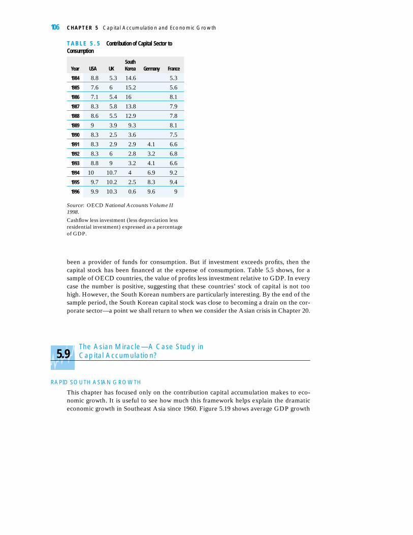
been a provider of funds for consumption. But if investment exceeds profits, then thecapital stock has been financed at the expense of consumption. Table 5.5 shows, for asample of OECD countries, the value of profits less investment relative to GDP. In everycase the number is positive, suggesting that these countries’ stock of capital is not toohigh. However, the South Korean numbers are particularly interesting. By the end of thesample period, the South Korean capital stock was close to becoming a drain on the cor-porate sector—a point we shall return to when we consider the Asian crisis in Chapter 20.

5.9The Asian Miracle—A Case Study inCapital Accumulation?

RAPID SOUTH ASIAN GROWTH

This chapter has focused only on the contribution capital accumulation makes to eco-nomic growth. It is useful to see how much this framework helps explain the dramaticeconomic growth in Southeast Asia since 1960. Figure 5.19 shows average GDP growth


T A B L E 5 . 5 Contribution of Capital Sector toConsumption

SouthYear USA UK Korea Germany France

1984 8.8 5.3 14.6 5.3

1985 7.6 6 15.2 5.6

1986 7.1 5.4 16 8.1

1987 8.3 5.8 13.8 7.9

1988 8.6 5.5 12.9 7.8

1989 9 3.9 9.3 8.1

1990 8.3 2.5 3.6 7.5

1991 8.3 2.9 2.9 4.1 6.6

1992 8.3 6 2.8 3.2 6.8

1993 8.8 9 3.2 4.1 6.6

1994 10. 10.7 4 6.9 9.2

1995 9.7 10.2 2.5 8.3 9.4

1996 9.9 10.3 0.6 9.6 9

Source: OECD National Accounts Volume II1998.

Cashflow less investment (less depreciation lessresidential investment) expressed as a percentageof GDP.

rate between 1966 and 1990 for a selection of countries. The performance of the AsianTigers over this period—Japan, Hong Kong, Singapore, Taiwan, and South Korea—was exceptional, with average growth rates in excess of 6% per annum.

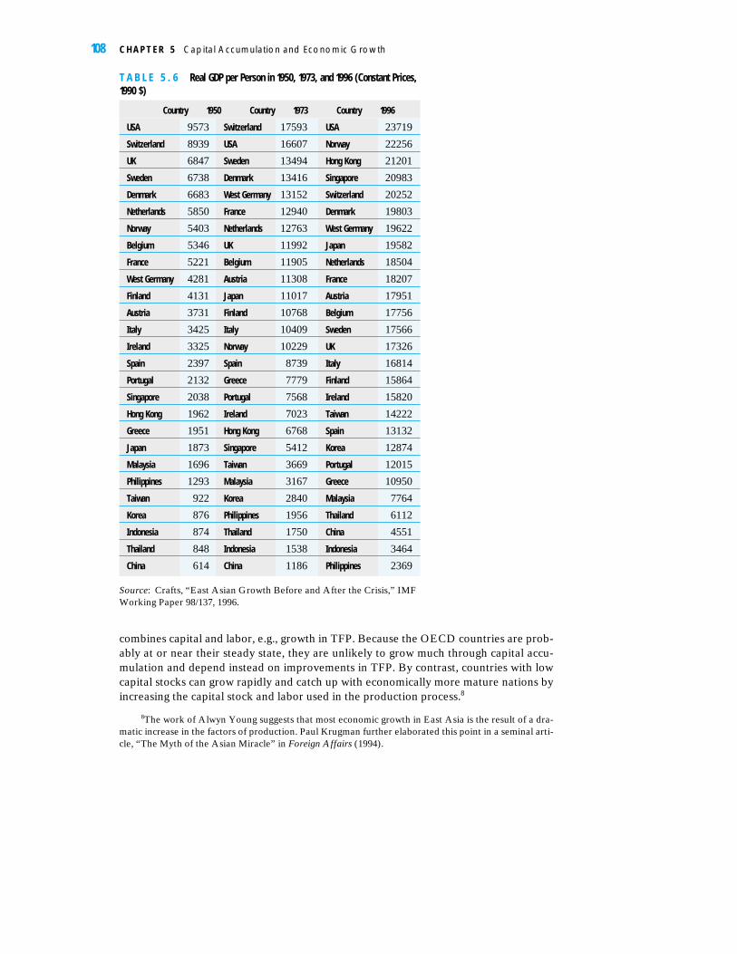
Such rapid increases in GDP have transformed the standard of living in theseeconomies. Table 5.6 lists real GDP per capita for a variety of OECD and Asianeconomies. In 1950 the wealthiest Asian country was Singapore, which was ranked sev-enteenth amongst our sample—slightly richer than the poorest European nation,Greece. Between 1950 and 1976, the European nations approximately doubled theirlevel of GDP per capita, but the Asian economies performed substantially better. Themost impressive growth occurred during 1973–1996. When the level of GDP per capitarose almost fourfold in Singapore, in less than one generation its standard of livingquadrupled. Most of the Asian economies experienced similar large increases in thestandard of living. By contrast, OECD nations saw relatively little growth—althoughIreland and Norway both doubled their standard of living, most other European coun-tries had only a 20–40% improvement. This “Asian miracle” and what the OECD na-tions could learn from it were much discussed by academics and by the media.

As Table 5.7 shows, the performance of these Asian countries really was excep-tional. In 1960 South Korea and Taiwan had a similar standard of living as Senegal,Ghana, and Mozambique. Between 1960 and 1990, these African countries had static ordeclining standards of living, whereas the Asian standards of living increased 6- or 7-fold. What made these Asian Tigers grow so fast, or alternatively, why didn’t growthlike this occur in Africa?

INCREASE THE INPUTS AND INCREASE THE OUTPUT

The production function implies that to increase output it is necessary to increase eitherfactor inputs, e.g., labor and capital, or the efficiency with which the production process

5.9 The Asian Miracle—A Case Study in Capital Accumulation? 107

0

ChileU.K.U.K.

GermanyMexicoFrance

CanadaBrazil

ItalyJapan

Hong KongSingapore

TaiwanSouth Korea

1 2 3 4 5 6 7

Ave

rage

GD

P p

er c

apita

grow

th 1

966

–69

F I G U R E 5 . 1 9 Growth in GDP per capita, 1966–90. The growth record of the Asian Tigers in the 25years from the mid 1960s was exceptional. Source: Summers and Heston, Penn World Table 5.5,http:/www.nber.org

combines capital and labor, e.g., growth in TFP. Because the OECD countries are prob-ably at or near their steady state, they are unlikely to grow much through capital accu-mulation and depend instead on improvements in TFP. By contrast, countries with lowcapital stocks can grow rapidly and catch up with economically more mature nations byincreasing the capital stock and labor used in the production process.8


8The work of Alwyn Young suggests that most economic growth in East Asia is the result of a dra-matic increase in the factors of production. Paul Krugman further elaborated this point in a seminal arti-cle, “The Myth of the Asian Miracle” in Foreign Affairs (1994).

T A B L E 5 . 6 Real GDP per Person in 1950, 1973, and 1996 (Constant Prices,1990 $)

Country 1950 Country 1973 Country 1996

USA 9573 Switzerland 17593 USA 23719

Switzerland 8939 USA 16607 Norway 22256

UK 6847 Sweden 13494 Hong Kong 21201

Sweden 6738 Denmark 13416 Singapore 20983

Denmark 6683 West Germany 13152 Switzerland 20252

Netherlands 5850 France 12940 Denmark 19803

Norway 5403 Netherlands 12763 West Germany 19622

Belgium 5346 UK 11992 Japan 19582

France 5221 Belgium 11905 Netherlands 18504

West Germany 4281 Austria 11308 France 18207

Finland 4131 Japan 11017 Austria 17951

Austria 3731 Finland 10768 Belgium 17756

Italy 3425 Italy 10409 Sweden 17566

Ireland 3325 Norway 10229 UK 17326

Spain 2397 Spain 8739 Italy 16814

Portugal 2132 Greece 7779 Finland 15864

Singapore 2038 Portugal 7568 Ireland 15820

Hong Kong 1962 Ireland 7023 Taiwan 14222

Greece 1951 Hong Kong 6768 Spain 13132

Japan 1873 Singapore 5412 Korea 12874

Malaysia 1696 Taiwan 3669 Portugal 12015

Philippines 1293 Malaysia 3167 Greece 10950

Taiwan 922 Korea 2840 Malaysia 7764

Korea 876 Philippines 1956 Thailand 6112

Indonesia 874 Thailand 1750 China 4551

Thailand 848 Indonesia 1538 Indonesia 3464

China 614 China 1186 Philippines 2369

Source: Crafts, “East Asian Growth Before and After the Crisis,” IMFWorking Paper 98/137, 1996.

The data supports this idea. For instance, Table 5.8 shows the higher average in-vestment rate in East Asian economies over 1981–1996 compared to the OECD num-bers in Table 5.4. Therefore we would expect more rapid growth in these SoutheastAsian economies for two reasons. First, they began with lower levels of capital, so as aresult of diminishing marginal product of capital, they should catch up with wealthiernations. Second, high investment rates mean the steady state level of capital is high.Therefore, as in Figure 5.16, the East Asian economies have further to grow beforethey reach their steady state.

Increases in capital are not the only explanation for this rapid Southeast Asiangrowth—other factors of production also increased. For instance, while OECD coun-tries were experiencing a declining birth rate and sometimes falling populations, theproportion of the Southeast Asian population aged between 15 and 64 years—the cru-cial working age population—was increasing rapidly. Average hours worked alsorose—see Table 5.9.

In a controversial study, Alwyn Young claimed that a growth accounting exercisefor these fast growing Southeast Asian economies suggests that growth was almost en-tirely due to capital accumulation and increased labor input (see Figure 5.20). For eachcountry the most important factor behind economic growth has been capital accumula-tion. TFP only contributed a substantial amount to economic growth in Hong Kong. InSingapore, Young calculates that TFP growth has actually been negative. In otherwords, Singapore should have witnessed an even larger increase in GDP given the ex-traordinary increase in capital and labor that occurred there. Young suggests this nega-tive TFP growth is a result of Singapore’s ambitious development plans. Thegovernment intervened in many facets of the economy—from the provision of compul-sory savings via the pension scheme to choosing which industries to develop. As a re-sult, the industrial structure has frequently changed, with the economy moving from


T A B L E 5 . 7 Asia and Africa in 1960

Country GDP per Capita 1960 GDP per Capita 1990

South Korea 883 6206

Taiwan 1359 6207

Ghana 873 815

Senegal 1017 1082

Mozambique 1128 756

Source: Summers and Heston, Penn World Table5.5, http:/www.nber.org

T A B L E 5 . 8 Asian Investment Rates, 1981–96

HongChina Kong Indonesia Korea Malaysia Philippines Singapore Taiwan Thailand

35.5 28.4 32.0 33.5 35.8 22.3 39.1 22.8 35.4

Source: Crafts, “East Asian Growth Before and After the Crisis,” IMF Working Paper98/137, 1996.

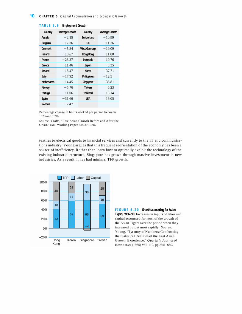
textiles to electrical goods to financial services and currently to the IT and communica-tions industry. Young argues that this frequent reorientation of the economy has been asource of inefficiency. Rather than learn how to optimally exploit the technology of theexisting industrial structure, Singapore has grown through massive investment in newindustries. As a result, it has had minimal TFP growth.


T A B L E 5 . 9 Employment Growth

Country Average Growth Country Average Growth

Austria �2.15 Switzerland �10.99

Belgium �17.36 UK �11.26

Denmark �5.34 West Germany �19.09

Finland �18.67 Hong Kong 11.80

France �23.37 Indonesia 19.76

Greece �11.46 Japan �8.35

Ireland �18.47 Korea 37.71

Italy �17.92 Philippines �12.5

Netherlands �14.45 Singapore 36.81

Norway �5.76 Taiwan 6.23

Portugal 11.06 Thailand 13.14

Spain �31.66 USA 19.05

Sweden �7.47

Percentage change in hours worked per person between1973 and 1996.

Source: Crafts, “East Asian Growth Before and After theCrisis,” IMF Working Paper 98/137, 1996.

TFP Labor Capital

0%

–20%

20%

40%

60%

80%

100%

HongKong

Korea Singapore Taiwan

42

18

4023

17

59 66

38

–4

53

19

28

F I G U R E 5 . 2 0 Growth accounting for AsianTigers, 1966–90. Increases in inputs of labor andcapital accounted for most of the growth ofthe Asian Tigers over the period when theyincreased output most rapidly. Source:Young, “Tyranny of Numbers: Confrontingthe Statistical Realities of the East AsianGrowth Experience,” Quarterly Journal ofEconomics (1985) vol. 110, pp. 641–680.

1963

1965

1967

1969

1971

1973

1975

1977

1979

1981

1983

1985

1987

1989

1991

0

10

20

30

40

50

Hong Kong

Singapore

Per

cent

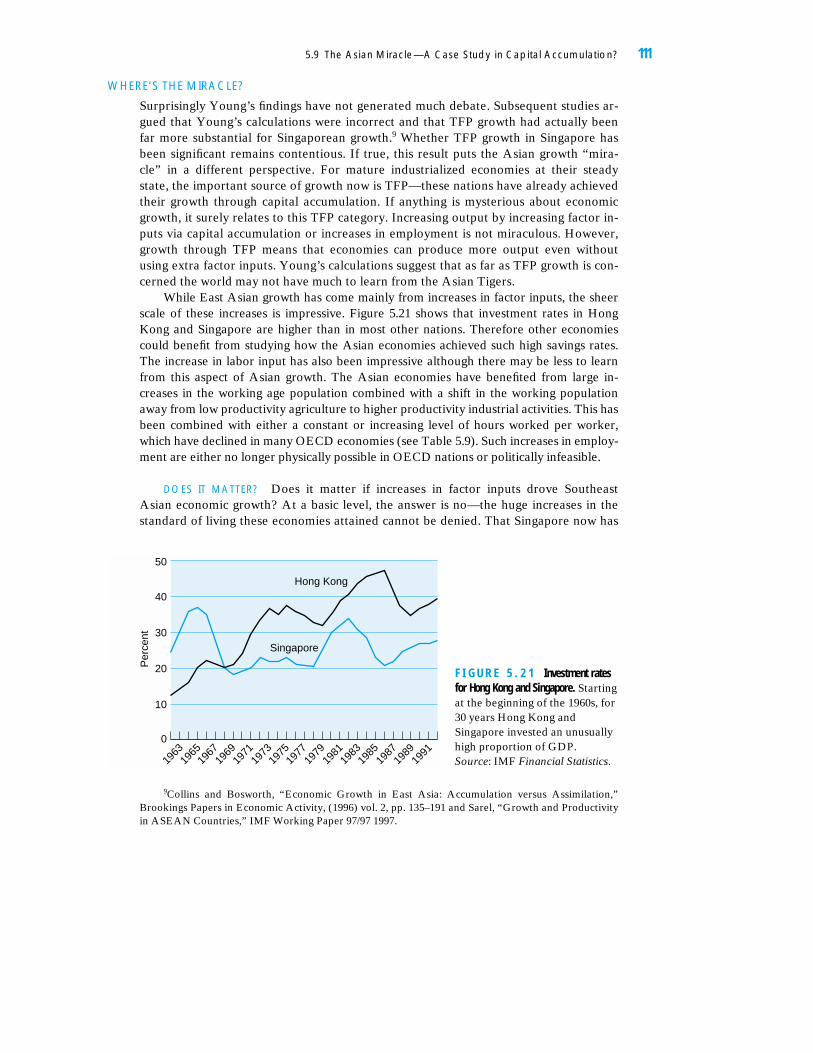
F I G U R E 5 . 2 1 Investment ratesfor Hong Kong and Singapore. Startingat the beginning of the 1960s, for30 years Hong Kong andSingapore invested an unusuallyhigh proportion of GDP.Source: IMF Financial Statistics.

WHERE’S THE MIRACLE?

Surprisingly Young’s findings have not generated much debate. Subsequent studies ar-gued that Young’s calculations were incorrect and that TFP growth had actually beenfar more substantial for Singaporean growth.9 Whether TFP growth in Singapore hasbeen significant remains contentious. If true, this result puts the Asian growth “mira-cle” in a different perspective. For mature industrialized economies at their steadystate, the important source of growth now is TFP—these nations have already achievedtheir growth through capital accumulation. If anything is mysterious about economicgrowth, it surely relates to this TFP category. Increasing output by increasing factor in-puts via capital accumulation or increases in employment is not miraculous. However,growth through TFP means that economies can produce more output even withoutusing extra factor inputs. Young’s calculations suggest that as far as TFP growth is con-cerned the world may not have much to learn from the Asian Tigers.

While East Asian growth has come mainly from increases in factor inputs, the sheerscale of these increases is impressive. Figure 5.21 shows that investment rates in HongKong and Singapore are higher than in most other nations. Therefore other economiescould benefit from studying how the Asian economies achieved such high savings rates.The increase in labor input has also been impressive although there may be less to learnfrom this aspect of Asian growth. The Asian economies have benefited from large in-creases in the working age population combined with a shift in the working populationaway from low productivity agriculture to higher productivity industrial activities. This hasbeen combined with either a constant or increasing level of hours worked per worker,which have declined in many OECD economies (see Table 5.9). Such increases in employ-ment are either no longer physically possible in OECD nations or politically infeasible.

DOES IT MATTER? Does it matter if increases in factor inputs drove SoutheastAsian economic growth? At a basic level, the answer is no—the huge increases in thestandard of living these economies attained cannot be denied. That Singapore now has


9Collins and Bosworth, “Economic Growth in East Asia: Accumulation versus Assimilation,”Brookings Papers in Economic Activity, (1996) vol. 2, pp. 135–191 and Sarel, “Growth and Productivityin ASEAN Countries,” IMF Working Paper 97/97 1997.

one of the highest standards of living in the world is not a statistical mirage. On theother hand, it does matter, for two reasons. The first is to emphasize that this growth hasnot been miraculous but has required sacrifices. Singapore has such high levels of capi-tal today because it had high investment rates in previous decades. Lower consumptionin previous decades paid for current prosperity. The current generation of Singaporeansare benefiting from these sacrifices, but their high standard of living has come at a cost.

The second reason for concern is the implications that decreasing marginal product ofcapital have for future economic growth in the region. If technology is characterized by de-creasing marginal product of capital, then the Asian Tigers will eventually reach theirsteady state, if they are not already there. Figure 5.22 shows Young’s calculations of themarginal product of capital and suggests that by the end of the 1980s decreasing marginalproduct had already set in. Because of their high investment rates, this steady state will beat high levels of output per head. However, once at this steady state the economy willcease to grow very fast through capital accumulation, and instead these countries will haveto pay attention to the factors that drive TFP. Just because Singapore, according toYoung’s calculations, has no history of strong TFP growth does not mean that it cannotproduce strong TFP growth in the future. However, our analysis suggests that at somepoint the development strategy of Singapore and the Asian Tigers will have to turn awayfrom just boosting factor inputs and focus on TFP improvements. For instance, between1966 and 1990 Singapore saw employment rise from 27% to 51% of the population, andinvestment as a proportion of GDP rose from 11% to 40%; in 1966 half the population hadno formal education, but by 1990 more than two thirds had completed secondary educa-tion. As a result of this huge improvement in factor inputs, the country witnessed remark-able growth. But a similar increase in factor inputs over the next 30 years is impossible.

5.10 China—A Big Tiger

The previous section suggested that Southeast Asia grew rapidly because of a sub-stantial increase in factor inputs based around high investment rates and a fast-growing


0 10 20 30 40 501966197019741975197619771978197919801981198219831984198519861987

Percent

F I G U R E 5 . 2 2 Real returnon capital in Singapore. As thecapital stock grew, the rateof return on capital inSingapore trended down.Source: Young, “Tyranny ofNumbers: Confronting theStatistical Realities of theEast Asian GrowthExperience,” QuarterlyJournal of Economics,(1985) vol. 110, pp. 641–680.

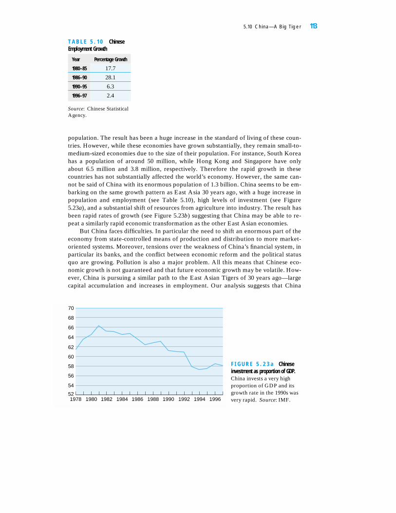
population. The result has been a huge increase in the standard of living of these coun-tries. However, while these economies have grown substantially, they remain small-to-medium-sized economies due to the size of their population. For instance, South Koreahas a population of around 50 million, while Hong Kong and Singapore have onlyabout 6.5 million and 3.8 million, respectively. Therefore the rapid growth in thesecountries has not substantially affected the world’s economy. However, the same can-not be said of China with its enormous population of 1.3 billion. China seems to be em-barking on the same growth pattern as East Asia 30 years ago, with a huge increase inpopulation and employment (see Table 5.10), high levels of investment (see Figure5.23a), and a substantial shift of resources from agriculture into industry. The result hasbeen rapid rates of growth (see Figure 5.23b) suggesting that China may be able to re-peat a similarly rapid economic transformation as the other East Asian economies.

But China faces difficulties. In particular the need to shift an enormous part of theeconomy from state-controlled means of production and distribution to more market-oriented systems. Moreover, tensions over the weakness of China’s financial system, inparticular its banks, and the conflict between economic reform and the political statusquo are growing. Pollution is also a major problem. All this means that Chinese eco-nomic growth is not guaranteed and that future economic growth may be volatile. How-ever, China is pursuing a similar path to the East Asian Tigers of 30 years ago—largecapital accumulation and increases in employment. Our analysis suggests that China

5.10 China—A Big Tiger 113

T A B L E 5 . 1 0 ChineseEmployment Growth

Year Percentage Growth

1980–85 17.7

1986–90 28.1

1990–95 6.3

1996–97 2.4

Source: Chinese StatisticalAgency.

1978 1980 1982 1984 1986 1988 1990 1992 1994 199652

54

56

58

60

62

64

66

68

70

F I G U R E 5 . 2 3 a Chineseinvestment as proportion of GDP.China invests a very highproportion of GDP and itsgrowth rate in the 1990s wasvery rapid. Source: IMF.

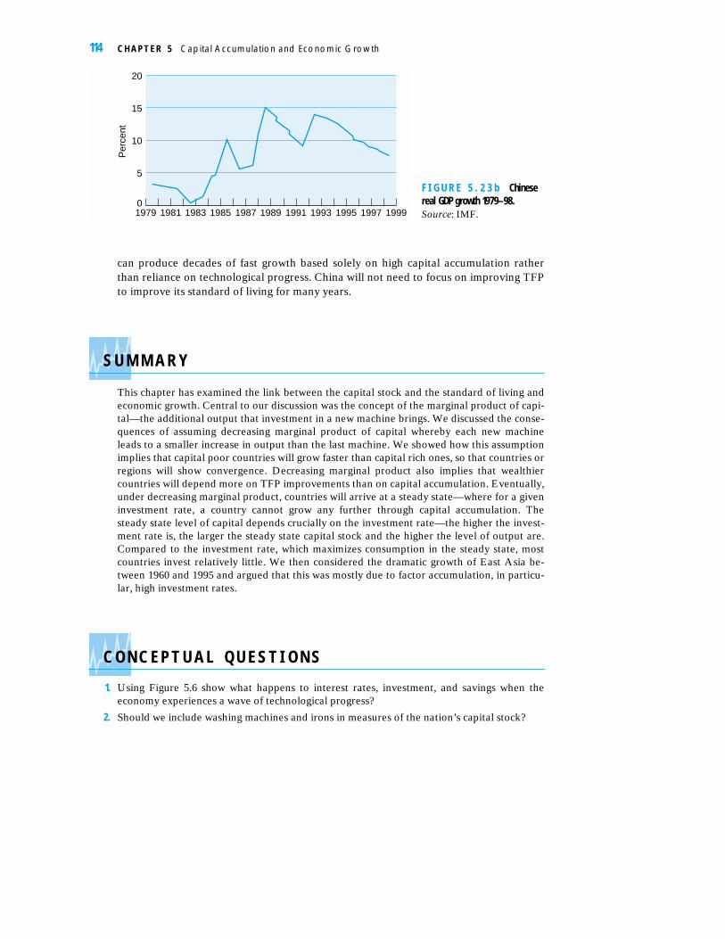
can produce decades of fast growth based solely on high capital accumulation ratherthan reliance on technological progress. China will not need to focus on improving TFPto improve its standard of living for many years.

S U M M A R Y

This chapter has examined the link between the capital stock and the standard of living andeconomic growth. Central to our discussion was the concept of the marginal product of capi-tal—the additional output that investment in a new machine brings. We discussed the conse-quences of assuming decreasing marginal product of capital whereby each new machineleads to a smaller increase in output than the last machine. We showed how this assumptionimplies that capital poor countries will grow faster than capital rich ones, so that countries orregions will show convergence. Decreasing marginal product also implies that wealthiercountries will depend more on TFP improvements than on capital accumulation. Eventually,under decreasing marginal product, countries will arrive at a steady state—where for a giveninvestment rate, a country cannot grow any further through capital accumulation. Thesteady state level of capital depends crucially on the investment rate—the higher the invest-ment rate is, the larger the steady state capital stock and the higher the level of output are.Compared to the investment rate, which maximizes consumption in the steady state, mostcountries invest relatively little. We then considered the dramatic growth of East Asia be-tween 1960 and 1995 and argued that this was mostly due to factor accumulation, in particu-lar, high investment rates.

C O N C E P T U A L Q U E S T I O N S

1. Using Figure 5.6 show what happens to interest rates, investment, and savings when theeconomy experiences a wave of technological progress?

2. Should we include washing machines and irons in measures of the nation’s capital stock?


1979 1981 1983 1985 1987 1989 1991 1993 1995 1997 19990

5

10

15

20

Per

cent

F I G U R E 5 . 2 3 b Chinesereal GDP growth 1979–98.Source: IMF.

3. What technologies might experience increasing marginal product of capital? Do they experi-ence increasing marginal product over all ranges?

4. What influences your savings decisions? How responsive would you be to tax incentives?

5. What can mature industrialized nations learn from the rapid growth of Southeast Asian na-tions?

6. A nation wishes to have a capital output ratio of 2 and has a depreciation rate of 10%. Whatinvestment rate should it aim for?

A N A L Y T I C A L Q U E S T I O N S

1. Gross investment in an economy (I) is a fixed proportion, �, of output (Y). Depreciation (D)is a fixed proportion, �, of the capital stock (K). What is the long-run impact of a rise in �from 0.15 to 0.20 if � is 0.05? What happens to the rate of return on capital if output is pro-duced with the Cobb-Douglas production function: Y � A. L0.7 K0.3?

2. The steady state level of consumption in an economy (Css) is equal to steady state output(Yss) minus steady state depreciation. The latter is the depreciation rate (�) times the steadystate capital stock (Kss). We assume here that there is no technological progress. Thus

Css � Yss � � Kss

What is the impact on steady state consumption of a small increase in the steady state capitalstock? What level of the capital stock maximizes the steady state rate of consumption?

3. The simple Golden Rule says that the optimal level of capital is one where the marginalproduct of capital equals the depreciation rate. If people attach less weight to the enjoymentthey get from consumption in the future than consumption today, then does it make sense toabide by the Golden Rule? Is there a better rule? If such an economy ever found itself withthe Golden Rule level of capital should it preserve the capital stock by setting gross invest-ment equal to depreciation?

4. Consider an economy where output (Y) is produced by labor (L) and capital (K) accordingto

Y � A. L0.7 K0.3

Investment is always 25% of output and the depreciation rate is 6%. If A � 10 and L � 100,what is the steady state level of K?

5. Suppose that the economy described in Question 4 enters the twenty-first century with acapital stock of 15,000. Assume that the labor force in year 2000 is 100 and remains constantand there is no technical progress. Calculate output and investment in 2000 and derive thecapital stock in 2001. Use the relation

Kt�1 � Kt � It � �Kt where � is the depreciation rate (� 0.06).

Then calculate output, investment, and the capital stock for each year up to 2005. Plot theevolution of the capital stock on a graph and show the steady state that you calculated inQuestion 4 on the same figure.

Analytical Questions 115

capital accumulation and economic growth this chapter we examine the relationship between increases...

Documents